Lorentzian Geodesic Flows and Interpolation between Hypersurfaces in Euclidean Spaces

Abstract.

We consider geodesic flows between hypersurfaces in ${\mathbb{R}}^{n}$. However, rather than consider using geodesics in ${\mathbb{R}}^{n}$, which are straight lines, we consider an induced flow using geodesics between the tangent spaces of the hypersurfaces viewed as affine hyperplanes. For naturality, we want the geodesic flow to be invariant under rigid transformations and homotheties. Consequently, we do not use the dual projective space, as the geodesic flow in this space is not preserved under translations. Instead we give an alternate approach using a Lorentzian space, which is semi-Riemannian with a metric of index $1$.

For this space for points corresponding to affine hyperplanes in ${\mathbb{R}}^{n}$, we give a formula for the geodesic between two such points. As a consequence, we show the geodesic flow is preserved by rigid transformations and homotheties of ${\mathbb{R}}^{n}$. Furthermore, we give a criterion that a vector field in a smoothly varying family of hyperplanes along a curve yields a Lorentzian parallel vector field for the corresponding curve in the Lorentzian space. As a result this provides a method to extend an orthogonal frame in one affine hyperplane to a smoothly “Lorentzian varying”family of orthogonal frames in a family of affine hyperplanes along a smooth curve, as well as a interpolating between two such frames with a smooth “minimally Lorentzian varying”family of orthogonal frames.

We further give sufficient conditions that the Lorentzian flow from a hypersurface is nonsingular and that the resulting corresponding flow in ${\mathbb{R}}^{n}$ is nonsingular. This is illustrated for surfaces in ${\mathbb{R}}^{3}$.

PRELIMINARY VERSION

Introduction

We consider the problem of constructing a natural diffeomorphic flow between hypersurfaces $M_{0}$ and $M_{1}$ of ${\mathbb{R}}^{n}$ which is in some sense both “natural”and “geodesic”viewed in some appropriate space (as in figure ).

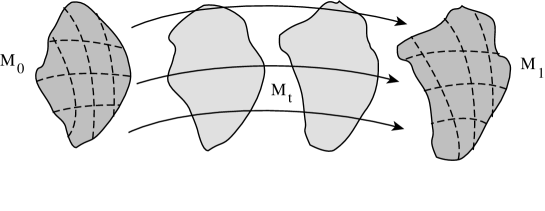
Figure 1. Diffeomorphic Flow between hypersurfaces of Euclidean space induced by a “Geodesic Flow”in an associated space

There are several approaches to this question. One is from the perspective of a Riemannian metric on the group of diffeomorphisms of ${\mathbb{R}}^{n}$. If the smooth hypersurfaces $M_{i}$ bound compact regions $\Omega_{i}$ , then the group of diffeomorphisms ${\rm Diff}\,({\mathbb{R}}^{n})$ acts on such regions $\Omega_{i}$ and their boundaries. Then, if $\varphi_{t},1\leq t\leq 1,$ is a geodesic in ${\rm Diff}\,({\mathbb{R}}^{n})$ beginning at the identity, then $\varphi_{t}(\Omega)$ (or $\varphi_{t}(M_{i})$) provides a path interpolating between $\Omega_{0}=\varphi_{0}(\Omega)=\Omega$ and $\Omega_{1}=\varphi_{1}(\Omega)$. Then, the geodesic equations can be computed and numerically solved to construct the flow $\varphi_{t}$. This is the method developed by Younes, Trouve, Glaunes [Tr], [YTG], [BMTY], [YTG2], and Mumford, Michor [MM], [MM2] etc.

An alternate approach which we consider in this paper requires that we are given a correspondence between $M_{0}$ and $M_{1}$, defined by a diffeomorphism $\chi:M_{0}\to M_{1}$, which need not be the restriction of a global diffeomorphism of ${\mathbb{R}}^{n}$ (and the $M_{i}$ may have boundaries). Then, if we map $M_{0}$ and $M_{1}$ to submanifolds of a natural ambient space $\Lambda$, we can seek a “geodesic flow”between $M_{0}$ and $M_{1}$, viewed as submanifolds of $\Lambda$, sending $x$ to $\varphi(x)$ along a geodesic. Then, we use this geodesic flow to define a flow between $M_{0}$ and $M_{1}$ back in ${\mathbb{R}}^{n}$.

The simplest example of this is the “radial flow”from $M_{0}$ using the vector field $U$ on $M_{0}$ defined by $U(x)=\varphi(x)-x$. Then, the radial flow is the geodesic flow in ${\mathbb{R}}^{n}$ defined by $\varphi_{t}(x)=x+t\cdot U(x)$. The analysis of the nonsingularity of the radial flow is given in [D1] in the more general context of “skeletal structures”. This includes the case where $M_{1}$ is a “generalized offset surface”of $M_{0}$ via the generalized offset vector field $U$.

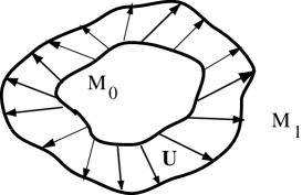
(a)                                         (b)

Figure 2. a) Hypersurface $M_{0}$ and radial vector field $U$ define a generalized offset surface $M_{1}$ obtained from a radial flow of the skeletal structure $(M_{0},U)$. This gives a nonsingular “Geodesic Flow”in ${\mathbb{R}}^{n}$. In b) there is no nonsingular geodesic flow in ${\mathbb{R}}^{n}$ from $M_{0}$ to $M_{1}$; however, there is a nonsingular Lorentzian geodesic flow from $M_{0}$ to $M_{1}$ (see §9)

In this paper, we give an alternate approach to interpolation via a geodesic flow between hypersurfaces with a given correspondence. While the radial flow views each hypersurface as a collection of points, we will instead view each as defined by their collection of tangent spaces. This leads to consideration of geodesic flows between “dual varieties”. The dual varieties traditionally lie in the “dual projective space”. However, the geodesic flow induced on the dual projective space with its natural Riemannian metric does not have certain natural properties that are desirable, such as invariance under translation. Instead, we shall define in §3 a ‘Lorentzian map”to a hypersurface $\mathcal{T}^{n}$ in the Lorentzian space $\Lambda^{n+1}$ defined by their tangent spaces as affine hyperplanes in ${\mathbb{R}}^{n+1}$. So instead of representing hypersurfaces in terms of “dual varieties”, we instead represent them as subspaces of $\Lambda^{n+1}$, which is the subspace of points in Minkowski space ${\mathbb{R}}^{n+2,1}$ of Lorentzian norm $1$. Then, we use the geodesic flow for the Lorentzian metric on $\Lambda^{n+1}$, and then transform that geodesic flow back to a flow between the original manifolds in ${\mathbb{R}}^{n}$.

To do this we determine in §4 the explicit form for the Lorentzian geodesics in $\Lambda^{n+1}$ between points in $\mathcal{T}^{n}$. We show these geodesics lie in $\mathcal{T}^{n}$ and show in §5 that these geodesics are invariant under the extended Poincare group. Given a Lorentzian geodesic between two points in $\mathcal{T}^{n}$, there corresponds a smooth family of hyperplanes $\Pi_{t}$.

We further give in §6 a criterion for “Lorentzian parallel vector fields”  in a family of hyperplanes $\Pi_{t}$ along a curve $\gamma(t)$ in ${\mathbb{R}}^{n}$, and then determine the Lorentzian parallel vector fields over a Lorentzian geodesic corresponding to vector fields with values in $\Pi_{t}$. Using this, we determine for an orthonormal frame $\{e_{i,0}\}$ in $\Pi_{0}$, a smooth family of orthonormal frames $\{e_{i,t}\}$ in $\Pi_{t}$ which correspond to a Lorentzian parallel family of frames along the Lorentzian geodesic. Using this we further determine a method for interpolating between orthonormal frames $\{e_{i,0}\}$ in $\Pi_{0}$ and $\{e_{i,1}\}$ in $\Pi_{1}$.

In §§7 and 8 we relate the properties of hypersurfaces $\tilde{M}$ of $\mathcal{T}^{n}$ with corresponding properties of the envelopes formed from the planes defined by $\tilde{M}$. In §7 we give a diffeomorphism between the Lorentzian space $\mathcal{T}^{n}$ with the dual projective space ${\mathbb{R}}P^{n\,\vee}$, which is a Riemannian manifold. The classification of generic Legendrian singularities in ${\mathbb{R}}P^{n\,\vee}$ gives the form of the singular points of images and this is used to give criteria for the lifting to a hypersurface in ${\mathbb{R}}^{n+1}$ as the envelope of the family of corresponding hyperplanes.

Finally, in section 9 we give in Theorem 9.2 the existence and continuous dependence of the corresponding “Lorentzian geodesic flow”  between two hypersurfaces $M_{0}$ and $M_{1}$ in ${\mathbb{R}}^{n+1}$ and in Theorem 9.3 we give a sufficient condition for the flow to be nonsingular. As a special case we consider in §10 the results for surfaces in ${\mathbb{R}}^{3}$.

CONTENTS

1. Overview

2. Semi-Riemannian Manifolds and Lorentzian Manifolds

3. Definition of the Lorentzian Map

4. Lorentzian Geodesic Flow on $\Lambda^{n+1}$

5. Invariance of Lorentzian Geodesic Flow and Special Cases

6. Families of Lorentzian Parallel Frames on Lorentzian Geodesic Flows

7. Dual Varieties and Singular Lorentzian Manifolds

8. Sufficient Condition for Smoothness of Envelopes

9. Induced Geodesic Flow between Hypersurfaces

10. Results for the Case of Surfaces in ${\mathbb{R}}^{3}$

1. Overview

As mentioned in the introduction there are two main methods for deforming one given hypersurface $M_{0}\subset{\mathbb{R}}^{n}$ to another $M_{1}$. One is to find a path $\psi_{t}$ in $G$, which is some specified a group of diffeomorphisms of ${\mathbb{R}}^{n}$, from the identity so that $\psi_{1}(M_{0})=M_{1}$ (and $\psi_{0}(M_{0})=M_{0}$).

Another approach involves constructing a geometric flow between $M_{0}$ and $M_{1}$. Several flows such as curvature flows do not provide a flow to a specific hypersurface such as $M_{1}$. An alternate approach which we shall use will assume that we have a correspondence given by a diffeomorphism $\chi:M_{0}\to M_{1}$ and construct a “geodesic flow”which at time $t=1$ gives $\chi$. The geodesic flow will be defined using an associated space $\mathcal{Y}$. We shall consider natural maps $\varphi_{i}:M_{i}\to\mathcal{Y}$ , where $\mathcal{Y}$ is a distinguished space which reflects certain geometric properties of the $M_{i}$.

$${M_{0}} \overset{\,\,\,\varphi_{0}}{\longrightarrow} \mathcal{Y}$$

(1.1) $${\chi\downarrow} \underset{\,\,\,\varphi_{1}}{\nearrow}$$

$${M_{1}}$$

Definition 1.1.

Given smooth maps $\varphi_{i}:M_{i}\to\mathcal{Y}$ and a diffeomorphism $\chi:M_{0}\to M_{1}$ A geodesic flow between the maps $\varphi_{i}$ is a smooth map $\tilde{\psi}_{t}:M_{0}\times[0,1]\to\mathcal{Y}$ such that for any $x\in M_{0}$, $\tilde{\psi}_{t}(x):[0,1]\to\mathcal{Y}$ is a geodesic from $\varphi_{0}(x)$ to $\varphi_{1}\circ\chi(x)$

Remark .

We shall also refer to the geodesic flow as being between the $\tilde{M}_{i}=\varphi_{i}(M_{i})$. However, we note that it is possible for more than one $x_{i}\in M_{0}$ to map to the same point in $y\in\mathcal{Y}$, however, the geodesic flow from $y$ can differ for each point $x_{i}$.

Then, we will complement this with a method for finding the corresponding flow $\psi_{t}$ between $M_{0}$ and $M_{1}$ such that $\varphi_{t}\circ\psi_{t}=\tilde{\psi}_{t}$, where $\varphi_{t}:\psi_{t}(M_{0})\to\tilde{\psi}_{t}(M_{0})$. We furthermore want this flow to satisfy certain properties. A main property is that the flow construction is invariant under the action of the extended Poincare group formed from rigid transformations and homotheties (scalar multiplication). By this we mean: if $M_{0}^{\prime}=A(M_{0})$ and $M_{1}^{\prime}=A(M_{1})$ are transforms of $M_{0}$ and $M_{1}$ by a transformation $A$ formed from the composition of a rigid transformation and homothety, and $M_{t}$ is the flow between $M_{0}$ and $M_{1}$, then $A(M_{t})$ gives the flow between $M_{0}^{\prime}$ and $M_{1}^{\prime}$.

We are specifically interested in a “geodesic flow”which will be a flow defined using the tangent bundles $TM_{0}$ to $TM_{1}$ so that we specifically control the flow of the tangent spaces. At first, an apparent natural choice is the dual projective space ${\mathbb{R}}P^{n\vee}$. Via the tangent bundle of a hypersurface $M\subset{\mathbb{R}}^{n}\,(\subset{\mathbb{R}}P^{n})$ there is the natural map $\delta:M\to{\mathbb{R}}P^{n\vee}$, sending $x\mapsto T_{x}M$. The natural Riemannian structure on the real projective space ${\mathbb{R}}P^{n\vee}$ is induced from $S^{n}$ via the natural covering map $S^{n}\to{\mathbb{R}}P^{n}$, so that geodesics of $S^{n}$ map to geodesics on ${\mathbb{R}}P^{n\vee}$. However, simple examples show that the induced geodesic slow on ${\mathbb{R}}P^{n\vee}$ is not invariant under translation in ${\mathbb{R}}^{n}$. For example, this Riemannian geodesic flow between the hyperplanes given by $\mathbf{n}\cdot\mathbf{x}=c_{0}$ and $\mathbf{n}\cdot\mathbf{x}=c_{1}$ is given by $\mathbf{n}\cdot\mathbf{x}=c_{t}$, where $c_{t}=\tan(t\arctan(c_{1})+(1-t)\arctan(c_{0}))$. It is easily seen that if we translate the two planes by adding a fixed amount $d$ to each $c_{i}$, then the corresponding formula does not give the translation of the first.

We will use an alternate space for $\mathcal{Y}$, namely, the Lorentzian space $\Lambda^{n+1}$ which is a Lorentzian subspace of Minkowski space ${\mathbb{R}}^{n+2,1}$. In fact the images will be in an $n$-dimensional submanifold $\mathcal{T}^{n}\subset\Lambda^{n+1}$. On $\Lambda^{n+1}$ it is classical that the geodesics are intersections with planes through the origin in ${\mathbb{R}}^{n+2,1}$. This allows a simple description of the geodesic flow on $\Lambda^{n+1}$. We transfer this flow to a flow on ${\mathbb{R}}^{n}$ using an inverse envelope construction, which reduces to solving systems of linear equations. We will give conditions for the smoothness of the inverse construction which uses knowledge of the generic Legendrian singularities.

We shall furthermore see that the construction is invariant under the action of rigid transformations and homotheties. In addition, uniform translations and homotheties will be geodesic flows, and a “pseudo rotation”which is a variant of uniform rotation is also a geodesic flow.

2. Semi-Riemannian Manifolds and Lorentzian Manifolds

A Semi-Riemannian manifold $M$ is a smooth manifold $M$, with a nondegenerate bilinear form $<\cdot,\cdot>_{x}$ on the tangent space $T_{x}M$, for eaxh $x\in M$ which smoothly varies with $x$. We do not require that $<\cdot,\cdot>_{x}$ be positive definite. We denote the index of $<\cdot,\cdot>_{(x)}$ by $\nu$. In the case that $\nu=1$, $M$ is referred to as a Lorentzian manifold.

A basic example is Minkowski space which (for our purposes) is ${\mathbb{R}}^{n+2}$ with bilinear form defined for $v=(v_{1},\dots,v_{n+2})$ and $w=(w_{1},\dots,v_{n+2})$

$$<v,w>_{L}\quad=\quad\sum_{i=1}^{n+1}v_{i}\cdot w_{i}-v_{n+2}\cdot w_{n+2}$$

There are a number of different notations for this Minkowski space. We shall use ${\mathbb{R}}^{n+2,1}$. We shall also use the notation $<\cdot,\cdot>_{L}$ for the Lorentzian inner product on ${\mathbb{R}}^{n+2,1}$.

A submanifold $N$ of a semi-Riemannian manifold $M$ is a semi-Riemannian submanifold if for each $x\in N$, the restriction of $<\cdot,\cdot>_{(x)}$ to $T_{x}N$ is nondegenerate. There are several important submanifolds of ${\mathbb{R}}^{n+2,1}$. One such is the Lorentzian submanifold

$$\Lambda^{n+1}\,\,=\,\,\{(v_{1},\dots,v_{n+2})\in{\mathbb{R}}^{n+2,1}:\sum_{i=1}^{n+1}v_{i}^{2}\,-\,v_{n+2}^{2}\,=\,1\},$$

which is called de Sitter space (see Fig. 3). A second important one is hyperbolic space ${\mathbb{H}}^{n+1}$ defined by

$${\mathbb{H}}^{n+1}\,\,=\,\,\{(v_{1},\dots,v_{n+2})\in{\mathbb{R}}^{n+2,1}:\sum_{i=1}^{n+1}v_{i}^{2}\,-\,v_{n+2}^{2}\,=\,-1\ \,\,\mbox{and }\,v_{n+2}>0\}.$$

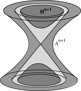
Figure 3. In Minkowski space ${\mathbb{R}}^{n+2,1}$, there is the Lorentzian hypersurface $\Lambda^{n+1}$ and the model for hyperbolic space ${\mathbb{H}}^{n+1}$. Also shown is the “light cone”.

By contrast the restriction of $<\cdot,\cdot>_{L}$ to ${\mathbb{H}}^{n+1}$ is a Riemannian metric of constant negative curvature $-1$. There is natural duality between codimension $1$ submanifolds of ${\mathbb{H}}^{n+1}$ obtained as the intersection of ${\mathbb{H}}^{n+1}$ with a “time-like”hyperplane $\Pi$ through $0$ (containing a “time-like”vector $z$ with $<z,z>_{L}\,<0$) paired with the points $\pm z^{\prime}\in\Lambda^{n+1}$ given where $z^{\prime}$ lies on a line through the origin which is the Lorentzian orthogonal complement to $\Pi$.

Many of the results which hold for Riemannian manifolds also hold for a Semi- Riemannian manifold $M$.

2.1Basic properties of Semi-Riemannian Manifolds (see [ON].

For a Semi-Riemannian manifold $M$, there are the following properties analogous to those for Riemannian manifolds:

1. Smooth Curves on $M$ have lengths defined using $|<\cdot,\cdot>|$.

2. There is a unique connection which satisfies the usual properties of a Riemannian Levi-Civita connection.

3. Geodesics are defined locally from any point $x\in M$ and with any initial velocity $v\in T_{x}M$. They are critical curves for the length functional, and they have constant speed.

4. If $N$ is a semi-Riemannian submanifold of $M$, then a constant speed curve $\gamma(t)$ in $N$ is a geodesic in $N$ if the acceleration $\gamma^{\prime\prime}(t)$ is normal to $N$ (with respect to the semi-Riemannian metric) at all points of $\gamma(t)$.

5. Any point $x\in M$ has a “convex neighborhood”  $W$, which has the property that any two points in $W$ are joined by a unique geodesic in the neighborhood.

6. If $\gamma(t)$ is a geodesic joining $x_{0}=\gamma(0)$ and $x_{1}=\gamma(1)$ and $x_{0}$ and $x_{1}$ are not conjugate along $\gamma(t)$, then given a neighborhood $W$ of $\gamma(t)$, there are neighborhoods of $W_{0}$ of $x_{0}$ and $W_{1}$ of $x_{1}$ so that if $x_{0}^{\prime}\in W_{0}$, and $x_{1}^{\prime}\in W_{1}$, there is a unique geodesic in the neighborhood $W$ from $x_{0}^{\prime}$ to $x_{1}^{\prime}$.

Then, as an example, it is straightforward to verify that for any $z\in\Lambda^{n+1}$, the vector $z$ is orthogonal to $\Lambda^{n+1}$ at the point $z$. Suppose $P$ is a plane in ${\mathbb{R}}^{n+2,1}$ containing the origin. Let $\gamma(t)$ be a constant Lorentzian speed parametrization of the curve obtained by intersecting $P$ with $\Lambda^{n+1}$. Then, by a standard argument similar to that for the case of a Euclidean sphere, $\gamma(t)$ is a geodesic. All geodesics of $\Lambda^{n+1}$ are obtained in this way. It follows that the submanifolds of $\Lambda^{n+1}$ obtained by intersecting $\Lambda^{n+1}$ with a linear subspace is a totally geodesic submanifold of $\Lambda^{n+1}$.

3. Definition of the Lorentzian Map

We begin by giving a geometric definition of a Lorentzian map from a smooth hypersurface $M\in{\mathbb{R}}^{n}$, as a natural map from $M$ to $\Lambda^{n+1}$; and then giving that geometric definition an algebraic form.

3.1. Geometric Definition of the Lorentzian Map

First, we let $S^{n}$ denote the unit sphere in ${\mathbb{R}}^{n+1}$ centered at the origin, and we let $\mathbf{e}_{n+1}=(0,\dots,0,1)\in{\mathbb{R}}^{n+1}$. Then, stereographic projection defines a map $p:S^{n}\backslash\{\mathbf{e}_{n+1}\}\to{\mathbb{R}}^{n}$ sending $y$ to the point where the line from $\mathbf{e}_{n+1}$ to $y$ intersects ${\mathbb{R}}^{n}$. Given a hyperplane $\Pi$ in ${\mathbb{R}}^{n}$, it together with $\mathbf{e}_{n+1}$ spans a hyperplane $\Pi^{\prime}$ in $R^{n+1}$. We can identify $R^{n+1}$ with $R^{n+1}\times\{\mathbf{e}_{n+2}\}\subset R^{n+2,1}$ by translation in the direction $\mathbf{e}_{n+2}$. The intersection of this plane with $S^{n+1}$ is an $n$-sphere. Then, via this identification of $R^{n+1}$ with the hyperplane in ${\mathbb{R}}^{n+2,1}$ defined by $x_{n+2}=1$, we form the hyperplane $\Pi^{\prime\prime}$ in ${\mathbb{R}}^{n+2,1}$ spanned by $\Pi^{\prime}$ together with $0$. This hyperplane is time-like because $\Pi^{\prime\prime}$ intersects $R^{n+1}\times\{\mathbf{e}_{n+2}\}$ in a hyperplane $\Pi^{\prime}$ which intersects the unit sphere in $R^{n+1}\times\{\mathbf{e}_{n+2}\}$ in a sphere, hence it intersects the interior disk. Then, the duality defined by the Lorentzian inner product associates to the hyperplane $\Pi^{\prime\prime}$ the Lorentzian orthogonal line $\ell$ through the origin. As the hyperplane is time-like, $\ell$ has non-empty intersection with $\Lambda^{n+1}$ in a pair of points $z$ and $-z$.

In order to obtain a single valued map, there are two possibilities: Either we consider the induce map to $\tilde{\Lambda}^{n+1}=\Lambda^{n+1}/\sim$, where $\sim$ identifies each pair of points $z$ and $-z$ of $\Lambda^{n+1}$; or we need on $\Pi$ a unit vector field $\mathbf{n}$ orienting $\Pi$. Given the normal vector $\mathbf{n}$, it defines a distinguished side of $\Pi$. Then we obtain a distinguished side for $\Pi^{\prime}$ and then $\Pi^{\prime\prime}$, which singles out one of the two points in $\Lambda^{n+1}$ on the distinguished side. We shall refer to this second case as the oriented case. We shall use both versions of the maps.

The geometric definition is then as follows.

Definition 3.1.

Given a smooth hypersurface $M\in{\mathbb{R}}^{n}$, with a smooth normal vector field $\mathbf{n}$ on $M$, the (oriented) Lorentz map is the natural map $\mathcal{L}:M\to\Lambda^{n+1}$ defined by $\mathcal{L}(x)=z$, where to $\Pi=T_{x}M$ is associated the plane $\Pi^{\prime\prime}$, Lorentzian orthogonal line $\ell$, and the distinguished intersection $z$ with $\Lambda^{n+1}$.

In the general case where we do not have an orientation for $M$, we define $\tilde{\mathcal{L}}:M\to\tilde{\Lambda}^{n+1}$ by $\tilde{\mathcal{L}}(x)$ is the equivalence class of $\pm z$ in $\tilde{\Lambda}^{n+1}$.

In fact, from the algebraic form of this map to follow, we shall see that it actually maps into an $n$ dimensional submanifold $\mathcal{T}^{n}$ of $\Lambda^{n+1}$. We give a specific algebraic form for this map.

3.2. Algebraic (Coordinate) Definition of the Lorentzian Map

We can give a coordinate definitions for the maps. If $T_{x}M$ is defined by $\mathbf{n}\cdot\mathbf{x}=c$, where $\mathbf{x}=(x_{1},\dots,x_{n})$. Then, $\Pi^{\prime}$ contains $T_{x}M$ and $\mathbf{e}_{n+1}$ and so is defined by $\mathbf{n}\cdot\mathbf{x}+cx_{n+1}=c$. Then, $\Pi^{\prime\prime}$ contains $\Pi^{\prime}\times\{\mathbf{e}_{n+2}\}$ and the origin so it is defined by $\mathbf{n}\cdot\mathbf{x}+cx_{n+1}-cx_{n+2}=0$. Thus, the Lorentzian orthogonal line $\ell$ is spanned by $(\mathbf{n},c,c)$, which we write in abbreviated form as $(\mathbf{n},c\boldsymbol{\epsilon})$ with $\boldsymbol{\epsilon}=(1,1)$. Hence, the map $\mathcal{L}:M\to\Lambda^{n+1}$ sends $x$ to $(\mathbf{n},c\boldsymbol{\epsilon})$, and the general case sends it to the equivalence class in $\tilde{\mathcal{T}}^{n}$ determined by $(\mathbf{n},c\boldsymbol{\epsilon})$. We shall be concerned with a subspace of $\Lambda^{n+1}$ where this duality corresponds to hypersurfaces of ${\mathbb{R}}^{n}$. The general correspondence is used in [OH] to parametrize $(n-1)$-dimensional spheres in ${\mathbb{R}}^{n}$.

We need on $M$ a smooth normal unit vector field $\mathbf{n}$ orienting $M$. Given the normal vector field $\mathbf{n}$, it defines a distinguished side of $T_{x}M$.

In fact, the image lies in the submanifold $\mathcal{T}^{n}$ of $\Lambda^{n+1}$ defined by

$$\mathcal{T}^{n}\quad=\quad\{(\mathbf{n},c\boldsymbol{\epsilon}):\mathbf{n}\in S^{n-1},c\in{\mathbb{R}}\}$$

which we can view as a submanifold $\mathcal{T}^{n}\subset\Lambda^{n+1}$; or in the general case it lies in $\tilde{\mathcal{T}}^{n}$.

Definition 3.2.

Given a smooth hypersurface $M\in{\mathbb{R}}^{n}$, with a smooth normal vector field $\mathbf{n}$ on $M$, the (oriented) Lorentz map is the natural map $\mathcal{L}:M\to\mathcal{T}^{n}$ defined by $\mathcal{L}(x)=(\mathbf{n},c\boldsymbol{\epsilon})$, where $T_{x}M$ is defined by $\mathbf{n}\cdot\mathbf{x}=c$. In the general case, we choose a local normal vector field and then $\tilde{\mathcal{L}}(x)$ is the equivalence class of $(\mathbf{n},c\boldsymbol{\epsilon})$ in $\tilde{\mathcal{T}}^{n}$.

In the following we shall generally concentrate on the oriented case and the map $\mathcal{L}$, with the general case just involving considering the map to equivalence classes.

Using $\mathcal{L}$ or $\tilde{\mathcal{L}}$, we are led to considering the geodesic flow in $\Lambda^{n+1}$, and obtain the induced geodesic flow on $\tilde{\Lambda}^{n+1}$. Once we have determined the geodesic flow between points in $\mathcal{T}^{n}$, there are two questions concerning $\mathcal{L}$ to lift the flow back to hypersurfaces in ${\mathbb{R}}^{n}$. One is when $\mathcal{L}$ is nonsingular, and at singular points what can we say about the local properties of $\mathcal{L}$ when $M$ is generic. The second question is how we may construct the inverse of $\mathcal{L}$ when it is a local embedding (or immersion).

4. Lorentzian Geodesic Flow on $\Lambda^{n+1}$

We give the general formula for the geodesic flow between points $z_{0}=(\mathbf{n}_{0},d_{0}\boldsymbol{\epsilon})$ and $z_{1}=(\mathbf{n}_{1},d_{1}\boldsymbol{\epsilon})$ in $\mathcal{T}^{n}$.

Several Auxiliary Functions

To do so we introduce several auxiliary functions. We first define the function $\lambda(x,\theta)$ by

(4.1) $$\lambda(x,\theta)\quad=\quad\Biggl{\{}\begin{matrix}\frac{\sin(x\theta)}{\sin(\theta)}\quad&\theta\neq 0\\ \,\,x\quad&\theta=0\end{matrix}\Biggr{.}$$

Then, $\sin(z)$ is a holomorphic function of $z$, and the quotient $\frac{\sin(x\theta)}{\sin(\theta)}$ has removable singularities along $\theta=0$ with value $x$. Hence, $\lambda(z,\theta)$ is a holomorphic function of $(z,\theta)$ on ${\mathbb{C}}\times((-\pi,\pi)\times\text{\it i}\,{\mathbb{R}})$, and so analytic on ${\mathbb{R}}\times(-\pi,\pi)$. Also, directly computing the derivative we obtain

(4.2) $$\dfrac{\partial\lambda((x,\theta)}{\partial x}\quad=\quad\Biggl{\{}\begin{matrix}\cos(x\theta)\cdot\frac{\theta}{\sin\theta}\quad&\theta\neq 0\\ \,\,1\quad&\theta=0\end{matrix}\Biggr{.}$$

Remark .

In fact, we can recognize $\lambda(n,\theta)$ for integer values $n$ as the characters for the irreducible representations of $SU(2)$ restricted to the maximal torus.

We also introduce a second function for later use in §5. For $-\frac{\pi}{2}<\theta<\frac{\pi}{2}$, we define

$$\mu(x,\theta)\,\,=\,\,\frac{\cos(x\theta)}{\cos(\theta)}.$$

Then, there is the following relation

(4.3) $$\lambda(x,\theta)+\lambda(1-x,\theta)\,\,=\,\,\mu(1-2x,\frac{\theta}{2})$$

This follows by using the basic trigonometric formulas $\sin(x)+\sin(y)=2\cos(\frac{1}{2}(x-y))\sin(\frac{1}{2}(x+y))$ and $\sin{\theta}=2\sin(\frac{1}{2}\theta)\cos(\frac{1}{2}\theta)$. There are additional relations between these two functions that follow from other basic trigonometric identies.   

Geodesic Curves in $\Lambda^{n+1}$ joining points in $\mathcal{T}^{n}$

We may express the geodesic curve between $z_{0}=(n_{0},c_{0}\epsilon)$ and $z_{1}=(n_{1},c_{1}\epsilon)$ in $\Lambda^{n+1}$ using $\lambda(x,\theta)$ provided $n_{1}\neq-n_{0}$. We let $-\frac{\pi}{2}<\theta<\frac{\pi}{2}$ be defined by $\cos\theta=\mathbf{n}_{0}\cdot\mathbf{n}_{1}$.

Proposition 4.1.

Provided $n_{1}\neq-n_{0}$, the geodesic curve $\gamma(t)$ in $\Lambda^{n+1}$ between points $\gamma(0)=z_{0}$ and $\gamma(1)=z_{1}$ in $\mathcal{T}^{n}$ for the Lorentzian metric on $\Lambda^{n+1}$ is given by

(4.4) $$\gamma(t)\quad=\quad\lambda(t,\theta)\,z_{1}\,+\,\lambda(1-t,\theta)\,z_{0}\qquad\mbox{for }0\leq t\leq 1$$

Furthermore, this curve lies in $\mathcal{T}^{n}$ for $0\leq t\leq 1$. Hence, $\mathcal{T}^{n}$ is a geodesic submanifold of $\Lambda^{n+1}$.

We can expand the expression for $\gamma(t)$ and obtain the family of hyperplanes $\Pi_{t}$ in ${\mathbb{R}}^{n}$. Expanding (4.4) we obtain

$$n_{t}\quad =\quad\lambda(t,\theta)\,\mathbf{n}_{1}\,+\,\lambda(1-t,\theta)\,\mathbf{n}_{0}\quad and$$

(4.5) $$c_{t}\quad =\quad\lambda(t,\theta)\,c_{1}\,+\,\lambda(1-t,\theta)\,c_{0}$$

Then the family $\Pi_{t}$ is given by

(4.6) $$\Pi_{t}\quad=\quad\{\mathbf{x}=(x_{1},\dots,x_{n})\in{\mathbb{R}}^{n}:\mathbf{x}\cdot\mathbf{n}_{t}=c_{t}\}$$

We can also compute the initial velocity for the geodesic in (4.4).

Corollary 4.2.

The initial velocity of the geodesic (4.4) with $\theta\neq 0$ is given by

(4.7) $$\gamma^{\prime}(0)\quad=\quad\frac{\theta}{\sin\theta}\cdot({\rm proj}_{\mathbf{n}_{0}}(\mathbf{n}_{1}),(c_{1}-\cos\theta\,c_{0})\boldsymbol{\epsilon})$$

where ${\rm proj}_{\mathbf{n}_{0}}$ denotes projection along $\mathbf{n}_{0}$ onto the line spanned by $\mathbf{w}$. If $\theta=0$, then $\mathbf{n}_{0}=\mathbf{n}_{1}$ and the velocity is $(0,(c_{1}-c_{0})\boldsymbol{\epsilon})$ (with Lorentzian speed $0$).

Remark .

Note that

$$\|({\rm proj}_{\mathbf{n}_{0}}(\mathbf{n}_{1}),(c_{1}-\cos\theta\,c_{0})\boldsymbol{\epsilon})\|_{L}\,\,=\,\,\|{\rm proj}_{\mathbf{n}_{0}}(\mathbf{n}_{1})\|$$

which equals $\sin\theta$. We conclude that the Lorentzian magnitude of $\gamma^{\prime}(0)$ is $\theta$. Since geodesics have constant speed, the geodesic will travel a distance $|\theta|$. Hence, $|\theta|$ is the Lorentzian distance between $z_{0}$ and $z_{1}$.

Proof of Proposition 4.1.

Let $P$ be the plane in ${\mathbb{R}}^{n+1,1}$ which contains $0$, $z_{0}$ and $z_{1}$. The geodesic curve between $z_{0}$ and $z_{1}$ is obtained as a constant Lorentzian speed parametrization of the curve obtained by intersecting $P$ with $\Lambda^{n+1}$. We choose a unit vector $\mathbf{w}\in\Pi$ such that $\mathbf{n}_{1}$ is in the plane through the origin spanned by $\mathbf{n}_{0}$ and $\mathbf{w}$. Let $0\leq\theta<\pi$ be the angle between $\mathbf{n}_{0}$ and $\mathbf{n}_{1}$ so $\cos\theta=\mathbf{n}_{0}\cdot\mathbf{n}_{1}$. Then, $\mathbf{n}_{1}-(\mathbf{n}_{1}\cdot\mathbf{n}_{0})\,\mathbf{n}_{0}$ is the projection of $\mathbf{n}_{1}$ along $\mathbf{n}_{0}$ onto the line spanned by $\mathbf{w}$ whose direction is chosen so that $\mathbf{n}_{1}-\cos\theta\,\mathbf{n}_{0}=\sin\theta\,\mathbf{w}$.

Then, a tangent vector to $\Lambda^{n+1}\cap P$ at the point $z_{0}$ is given by

(4.8) $$(\mathbf{n}_{1}-\cos\theta\,\mathbf{n}_{0},(c_{1}-\cos\theta\,c_{0})\boldsymbol{\epsilon})=(\sin\theta\,\mathbf{w},(c_{1}-\cos\theta\,c_{0})\boldsymbol{\epsilon})$$

Then, we seek a Lorentzian geodesic $\gamma(t)$ in the plane $P$ beginning at $(\mathbf{n}_{0},c_{0}\boldsymbol{\epsilon})$ with initial velocity in the direction $(\sin\theta\,\mathbf{w},(c_{1}-\cos\theta\,c_{0})\boldsymbol{\epsilon})$. Consider the curve

(4.9) $$\gamma(t)\,\,=\,\,(\cos(t\theta)\mathbf{n}_{0}\,+\,\sin(t\theta)\mathbf{w},(\cos(t\theta)c_{0}\,+\,\frac{\sin(t\theta)}{\sin(\theta)}(c_{1}-\cos\theta\,c_{0}))\boldsymbol{\epsilon})$$

First, note that $\gamma(0)=z_{0}$, and $\gamma(1)=z_{1}$. Also, this curve lies in the plane spanned by $z_{0}$ and (4.8). Also,

$$\|\gamma(t)\|_{L}\,\,=\,\,\|\cos(t\theta)\mathbf{n}_{0}\,+\,\sin(t\theta)\mathbf{w}\|\,\,=\,\,1$$

as $\mathbf{n}_{0}$ and $\mathbf{w}$ are orthogonal unit vectors. Hence, $\gamma(t)$ is a curve parametrizing $\Lambda^{n+1}\cap P$. It remains to show that $\gamma^{\prime\prime}$ is Lorentzian orthogonal to $\Lambda^{n+1}$ to establish that it is a Lorentzian geodesic from $z_{0}$ to $z_{1}$. A computation shows

$$\gamma^{\prime\prime}(t)\,\,=\,\,-\theta^{2}(\cos(t\theta)\mathbf{n}_{0}\,+\,\sin(t\theta)\mathbf{w},\frac{\sin(t\theta)}{\sin(\theta)}(c_{1}-\cos\theta\,c_{0})\boldsymbol{\epsilon})$$

which is $-\theta^{2}\gamma(t)$, and hence Lorentzian orthogonal to $\Lambda^{n+1}$.

Because of the fraction $\frac{\sin(t\theta)}{\sin(\theta)}$, we have to note that when $\theta=0$, then $\mathbf{n}_{0}=\mathbf{n}_{1}$ and $\gamma(t)$ takes the simplified form

$$\gamma(t)\,\,=\,\,(\mathbf{n}_{0},c_{0}\,+\,t(c_{1}-c_{0}))\boldsymbol{\epsilon})$$

which is still a Lorentzian geodesic between $z_{0}$ to $z_{1}$.

Lastly, we must show that this agrees with (4.4). First, consider the case where $\theta\neq 0$.

$$\mathbf{w}=\frac{1}{\sin\theta}\,(\mathbf{n}_{1}-\cos\theta\,\mathbf{n}_{0})$$

Substituting this into the first term of the RHS of (4.9), we obtain

$$\frac{1}{\sin\theta}(\sin\theta\,\cos(t\theta)-\cos\theta\,\sin(t\theta))\,\mathbf{n}_{0}\,+\,\frac{sin(t\theta)}{\sin\theta}\,\mathbf{n}_{1}$$

which by the formula for the sine of the difference of two angles equals

$$\frac{\sin((1-t)\theta)}{\sin\theta}\mathbf{n}_{0}\,+\frac{sin(t\theta)}{\sin\theta}\mathbf{n}_{1}$$

Analogously, we can compute the second term in the RHS of (4.9), to be

$$\frac{\sin((1-t)\theta)}{\sin\theta}c_{0}\,+\frac{sin(t\theta)}{\sin\theta}c_{1}$$

This gives (4.4) when $\theta\neq 0$. When $\theta=0$, $\mathbf{n}_{0}=\mathbf{n}_{1}$ and the derivation of (4.4) from (4.9) for $\theta=0$ is easier. ∎

Remark 4.3.

We have alread seen that the geodesic flow between the planes $\mathbf{n}_{0}\cdot x=c_{0}$ and $\mathbf{n}_{1}\cdot x=c_{1}$ induced from the geodesic flow in ${\mathbb{R}}P^{n\vee}$ corresponds to the geodesic flow between $(\mathbf{n}_{0},c_{0})$ and $(\mathbf{n}_{1},c_{1})$, which is given by the unit speed curve in the intersection of the plane $P$, containing these points and the origin, with the unit sphere $S^{n}$. If we replaced (4.4) by linear interpolation

(4.10) $$\gamma(t)\quad=\quad t\,(\mathbf{n}_{1},c_{1})\,+\,(1-t)\,(\mathbf{n}_{0},c_{0})\qquad\mbox{for }0\leq t\leq 1$$

then the curve lies in the plane $P$ and its projection onto the unit sphere does parametrize the geodesic, but it is not unit speed, and as we remarked earlier it is not invariant under translation and hence not under rigid transformations.

5. Invariance of Lorentzian Geodesic Flow and Special Cases

We investigate the invariance properties of Lorentzian geodesic flows and the properties of these flows in special cases.

Invariance of Lorentzian Geodesic Flow

We first claim the Geodesic flow given in Proposition 4.1 is invariant under the extended Poincare group generated by rigid transformations and scalar multiplications. By this we mean the following. If $\gamma(t)=(\mathbf{n}_{t},c_{t})$ is the Lorentzian geodesic flow between hyperplanes $P_{0}$ and $P_{1}$ defined by $\mathbf{n}_{0}\cdot x=c_{0}$, respectively $\mathbf{n}_{1}\cdot x=c_{1}$, then $\tilde{\psi}(\gamma(t))$ is the Lorentzian geodesic flow between hyperplanes $\psi(P_{0})$ and $\psi(P_{1})$.

Proposition 5.1.

The Lorentzian geodesic flow is invariant under the extended Poincare group.

Proof.

Suppose $z_{i}=(\mathbf{n}_{i},c_{i})\in\mathcal{T}^{n}$, i = 1, 2, and let $\Pi_{i}$ be the hyperplane determined by $z_{i}$. Let $\psi$ be an alement of the extended Poincare group. It is a composition of scalar multiplication by $b$ followed by a rigid transformation so $\psi(\mathbf{x})=b\,A(\mathbf{x})+\mathbf{p}$, with $A$ an orthogonal transformation. Then, $\Pi_{i}^{\prime}=\psi(\Pi_{i})$ is defined by

(5.1) $$\tilde{\psi}(z_{i})=\tilde{\psi}(\mathbf{n}_{i},c_{i})=(A(\mathbf{n}_{i}),bc_{i}+\mathbf{n}_{i}\cdot\mathbf{p}).$$

If $\cos(\theta)=\mathbf{n}_{0}\cdot\mathbf{n}_{1}$, then by (4.4) the Lorentzian geodesic flow is given by $\gamma(t)$ defined by

(5.2) $$(\mathbf{n}_{t},c_{t})\,\,=\,\,(\lambda(t,\theta)\mathbf{n}_{1}\,+\,\lambda(1-t,\theta)\,\mathbf{n}_{0},\,\,\lambda(t,\theta)\,c_{1}\,+\,\lambda(1-t,\theta)\,c_{0})$$

defining the family of hyperplanes $\Pi_{t}$. Then, by (5.1) $\Pi_{t}^{\prime}=\psi(\Pi_{t})$ is defined by $\mathbf{n}^{\prime}_{t}\cdot x=c^{\prime}_{t}$, where $\tilde{\psi}(\gamma(t))$ is defined by

(5.3) $$(\mathbf{n}^{\prime}_{t},c^{\prime}_{t})\,\, =\,\,\left(A(\lambda(t,\theta)\mathbf{n}_{1}\,+\,\lambda(1-t,\theta)\,\mathbf{n}_{0}),\,b(\lambda(t,\theta))c_{1}+\lambda(1-t,\theta))c_{0})\,+\right.$$

$$\qquad\qquad\,\left.A(\lambda(t,\theta)\mathbf{n}_{1}\,+\,\lambda(1-t,\theta)\cdot\mathbf{p})\right)$$

$$=\,\,\lambda(t,\theta)\left(A(\mathbf{n}_{1}),\,bc_{1}+A(\mathbf{n}_{1})\cdot\mathbf{p}\right)\,+\,\lambda(1-t,\theta)\left(A(\mathbf{n}_{0}),\,bc_{0}+A(\mathbf{n}_{0})\cdot\mathbf{p}\right)$$

$$=\,\,\lambda(1-t,\theta)\tilde{\psi}(z_{1})+\lambda(1-t,\theta)\tilde{\psi}(z_{0})$$

which is the geodesic flow between $\Pi_{0}^{\prime}$ defined by $\tilde{\psi}(z_{0})$ and $\Pi_{1}^{\prime}$ defined by $\tilde{\psi}(z_{1})$.

∎

Remark 5.2.

An alternate way to understand Proposition 4.1 is to observe that the extended Poincare group acts on ${\mathbb{R}}^{n}\times{\mathbb{R}}\epsilon$ sending $(\mathbf{v},c\epsilon)\mapsto(A(\mathbf{v}),(bc+\mathbf{v}\cdot\mathbf{w})\epsilon)$. This action preserves the Lorentzian inner product on this subspace and preserves $\mathcal{T}^{n}$. Hence, it maps geodesics in $\mathcal{T}^{n}$ to geodesics in $\mathcal{T}^{n}$.

Special Cases of Lorentzian Geodesic Flow

We next determine the form of the Lorentzian geodesic flow in several special cases.

Example 5.3 (Hypersurfaces Obtained by a Translation and Homothety).

Suppose that we obtain $\Pi_{1}$ from $\Pi_{0}$ by translation by a vector $\mathbf{p}$ and multiplication by a scalar $b$. The correspondence associates to $\mathbf{x}\in\Pi_{0}$, $bx^{\prime}=\mathbf{x}+\mathbf{p}\in\Pi_{1}$. Then, the geodesic flow is given by the following.

Corollary 5.4.

Suppose $\Pi_{0}$ is the hyperplane defined by $\mathbf{n}_{0}\cdot x=c_{0}$, with $\mathbf{n}_{0}$ a unit vector, and $\Pi_{1}$ is obtained from $\Pi_{0}$ by multiplication by the scalar $b\neq 0$ and then translation by $\mathbf{p}$. Then the Lorentzian geodesic flow $\Pi_{t}$ is given by the family of parallel hyperplanes defined by $\mathbf{n}_{0}\cdot x=c_{t}$ where $c_{t}=(1+(b-1)t)c_{0}+t\mathbf{n}_{0}\cdot\mathbf{p}$.

Proof.

If $\Pi_{0}$ is defined by $\mathbf{n}_{0}\cdot x=c_{0}$, with $\mathbf{n}_{0}$ a unit vector, then, $\Pi_{1}$ is defined by $\mathbf{n}_{1}\cdot x=c_{1}$ where $\mathbf{n}_{1}=\mathbf{n}_{0}$ and $c_{1}=bc_{0}+\mathbf{n}_{0}\cdot\mathbf{p}$. Thus, $\Pi_{1}$ is parallel to $\Pi_{0}$.

Thus, as $\mathbf{n}_{1}=\mathbf{n}_{0}$, $\theta=0$ and $\lambda(t,0)=t$, so the geodesic flow $\Pi_{t}$ is given by

$$t(\mathbf{n}_{0},c_{1}\boldsymbol{\epsilon})+(1-t)(\mathbf{n}_{0},c_{0}\boldsymbol{\epsilon})\,\, =\,\,(\mathbf{n}_{0},((1-t)c_{0}+t(bc_{0}+\mathbf{n}_{0}\cdot\mathbf{p}))\boldsymbol{\epsilon})$$

(5.4) $$=\,\,(\mathbf{n}_{0},((tb+1-t)c_{0}+t(\mathbf{n}_{0}\cdot\mathbf{p}))\boldsymbol{\epsilon})$$

so that $\Pi_{t}$ is defined by $\mathbf{n}_{0}\cdot\mathbf{x}=c_{t}$ where $c_{t}=(1+(b-1)t)c_{0}+t(\mathbf{n}_{0}\cdot\mathbf{p})$.

This defines a family of hyperplanes parallel to $\Pi_{0}$ where derivative of the translation map is the identity; hence, under translation $\mathbf{n}_{0}$ is mapped to itself translated to $\mathbf{x}^{\prime}=\mathbf{x}+\mathbf{p}$. Thus, under the correspondence, $\mathbf{n}_{1}=\mathbf{n}_{0}$. Also, If $\mathbf{n}_{0}\cdot\mathbf{x}=c_{0}$ is the equation of the tangent plane for $M_{0}$ at a point $\mathbf{x}$, then the tangent plane of $M_{1}$ at the point $\mathbf{x}^{\prime}$ is

$$\mathbf{n}_{1}\cdot\mathbf{x}^{\prime}\,=\,\mathbf{n}_{0}\cdot(\mathbf{x}+\mathbf{p})\,=\,c_{0}+\mathbf{n}_{0}\cdot\mathbf{p}$$

Hence, $c_{1}=c_{0}+\mathbf{n}_{0}\cdot\mathbf{p}$.

As $\mathbf{n}_{0}=\mathbf{n}_{1}$, $\theta=0$. Thus the geodesic flow on $\mathcal{T}^{n}$ is given by

$$t(\mathbf{n}_{0},c_{1}\boldsymbol{\epsilon})+(1-t)(\mathbf{n}_{0},c_{0}\boldsymbol{\epsilon})\,\,=\,\,(\mathbf{n}_{0},c_{0}\boldsymbol{\epsilon})+(0,(t\mathbf{n}_{0}\cdot\mathbf{p})\boldsymbol{\epsilon})\,\,=\,\,(\mathbf{n}_{0},(\mathbf{n}_{0}\cdot(\mathbf{x}+t\mathbf{p}))\boldsymbol{\epsilon})$$

Thus, at time $t$ the tangent space is translated by $t\mathbf{p}$. Thus, the envelope of these translated hyperplanes is the translation of $M_{0}$ by $t\mathbf{p}$. ∎

Remark 5.5.

If a hypersurface $M_{1}$ is obtained from the hypersurface $M_{0}$ by a translation combined with a homothety $\mathbf{x}^{\prime}=\psi(\mathbf{x})=b\mathbf{x}+\mathbf{p}$, then for each $x\in M_{0}$ with image $x^{\prime}\in M_{1}$ the Lorentzian geodesic flow will send the tangent plane $T_{x}M_{0}$ to the tangent plane $T_{x^{\prime}}M_{1}$ by the family of parallel hyperplanes given by Corollary 5.4. Thus, for each $0\leq t\leq 1$, the hyperplane under the geodesic flow will be the tangent plane $T_{\mathbf{x}_{t}}M_{t}$, where for $\psi_{t}(\mathbf{x})=(1+(b-1)t)\mathbf{x}+t\mathbf{p}$, $M_{t}=\psi_{t}(M_{0})$ and $\mathbf{x}_{t}=\psi_{t}(\mathbf{x})\in M_{t}$. Thus, the Lorentzian geodesic flow will send $M_{0}$ to the family of hypersurfaces $M_{t}=\psi_{t}(M_{0})$.

Example 5.6 (Hyperplanes Obtained by a Pseudo-Rotation).

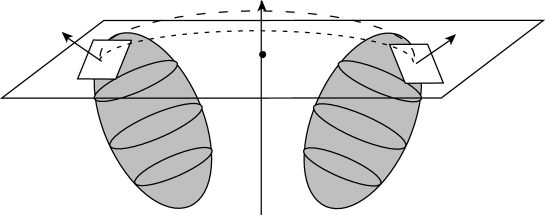
Figure 4. Lorentzian Geodesic Flow between a hyperplane $\Pi_{0}$ and a rotated copy $\Pi_{1}$, where the rotation is about a subspace not containing $W=\Pi_{0}\cap\Pi_{1}$, is given by a “pseudo–rotation”. The path of the rotation is indicated by the dotted curve, while that for the pseudo rotation is given by the curve, which lifts out of the plane of rotation before returning to it (although it does remain in a plane parallel to $W^{\perp}$).

Second, suppose that $\Pi_{0}$ and $\Pi_{1}$ are nonparallel affine hyperplanes. Then, $W=\Pi_{0}\cap\Pi_{1}$ is a codimension $2$ affine subspace. The unit normal vectors $\mathbf{n}_{0}$ and $\mathbf{n}_{1}$ lie in the orthogonal plane $W^{\perp}$ with $\mathbf{n}_{0}\cdot\mathbf{n}_{1}=\cos(\theta)$ with $-\pi/2<\theta<\pi/2$. Since the Lorentzian geodesic flow commutes with translation, we may translate the planes and assume that $W$ contains the origin. Then, both $c_{0}$ and $c_{1}$ equal $0$. Thus, by Proposition 4.1, the Lorentzian geodesic flow from $\Pi_{0}$ to $\Pi_{1}$ is given by $(\mathbf{n}_{t},c_{t}\boldsymbol{\epsilon})$ for $0\leq t\leq 1$, where

(5.5) $$(\mathbf{n}_{t},c_{t}\boldsymbol{\epsilon})\,\,=\,\,(\lambda(t,\theta)\,(\mathbf{n}_{1},c_{1}\boldsymbol{\epsilon})\,+\,\lambda(1-t,\theta)\,(\mathbf{n}_{0},c_{0}\boldsymbol{\epsilon})$$

Thus, $\mathbf{n}_{t}=\lambda(t,\theta)\mathbf{n}_{1}+\lambda(1-t,\theta)\mathbf{n}_{0}$, while $c_{t}\equiv 0$. Hence, the hyperplane $\Pi_{t}$ is defined by $\mathbf{n}_{t}\cdot\mathbf{x}=0$ so it contains $W$. However, its intersection with the plane $W^{\perp}$ is the line orthogonal to $\mathbf{n}_{t}$, which by the above expression for $\mathbf{n}_{t}$, does not give a standard constant speed rotation in the plane. We refer to this as a pseudo-rotation.

Instead consider a rotation $A$ of hyperplanes $\Pi_{0}$ to $\Pi_{1}$ about an axis not containing $W$. We consider the form of the pseudo-rotation. As an example, consider the case of a rotation $A$ about the origin in a plane (which pointwise fixes an orthogonal subspace. Choosing coordinates, we may assume that the rotation $A$ is in the $(x_{1},x_{2})$–plane and rotates by an angle $\omega$. We suppose $\Pi_{0}$, defined by $\mathbf{n}_{0}\cdot\mathbf{x}=c_{0}$. As $A(\mathbf{n}_{0})\cdot A(\mathbf{x})=\mathbf{n}_{0}\cdot\mathbf{x}=c_{0}$, if we let $\mathbf{x}^{\prime}=A(\mathbf{x})$, then the equation of the hyperplane $\Pi_{1}$ is defined by $A(\mathbf{n}_{0})\cdot\mathbf{x}^{\prime}=c_{0}$. Hence, $\mathbf{n}_{1}=A(\mathbf{n}_{0})$ and $c_{1}=c_{0}$.

To express the geodesic flow, we write $\mathbf{n}_{0}=\mathbf{v}+\mathbf{p}$ where $\mathbf{v}$ is in the rotation plane and $\mathbf{p}$ is fixed by $A$. Hence, $\mathbf{n}_{1}=A(\mathbf{v})+\mathbf{p}$. Thus, the angle $\theta$ between $\mathbf{n}_{0}$ and $\mathbf{n}_{1}$ satisfies

$$\cos\theta\,=\,\mathbf{n}_{1}\cdot\mathbf{n}_{0}\,=\,A(\mathbf{v})\cdot\mathbf{v}\,+\,\mathbf{p}\cdot\mathbf{p}$$

As $\|\mathbf{n}_{0}\|=1$, we obtain $\mathbf{v}\cdot\mathbf{v}\,+\,\mathbf{p}\cdot\mathbf{p}=1$. Also, $A(\mathbf{v})\cdot\mathbf{v}=\|\mathbf{v}\|^{2}\cos\omega$. Hence,

(5.6) $$\cos\theta\,=\,1+\|\mathbf{v}\|^{2}(\cos\omega-1)$$

We recall that by (4.3)

$$\lambda(t,\theta)+\lambda(1-t,\theta)\,\,=\,\,\mu(1-2t,\frac{\theta}{2})$$

Using the expressions for $\mathbf{n}_{0}$ and $\mathbf{n}_{1}$, we find the geodesic flow is given by

$$=\,\,\lambda(t,\theta)\,(A(\mathbf{n}_{0}),c_{0}\boldsymbol{\epsilon})+\lambda(1-t,\theta)\,(\mathbf{n}_{0},c_{0}\boldsymbol{\epsilon})$$

(5.7) $$=\,\,((\lambda(t,\theta)A(\mathbf{v})+\lambda(1-t,\theta)\,\mathbf{v})\,+\,\mu(1-2t,\frac{\theta}{2})\,\mathbf{p},\,\,\mu(1-2t,\frac{\theta}{2})c_{0}\boldsymbol{\epsilon})$$

We note that $\mu(1-2t,\frac{\theta}{2})$ is a function of $t$ on $[0,1]$ which has value $=1$ at the end points, and has a maximum $=\sec(\frac{1}{2}\theta)$ at $t=\frac{1}{2}$. Thus, the geodesic flow $(\mathbf{n}_{t},c_{t}\boldsymbol{\epsilon})$ has the contribution in the rotation plane given by $\lambda(t,\theta)A(\mathbf{v})+\lambda(1-t,\theta)\mathbf{v}$ which is not a true rotation from $\mathbf{v}$ to $A(\mathbf{v})$. Also, the other contribution to $\mathbf{n}_{t}$ is from $\mu(1-2t,\frac{\theta}{2})\mathbf{p}$ which increases and then returns to size $\mathbf{p}$ (see Fig. 4). In addition, the distance from the origin will vary by $\mu(1-2t,\frac{\theta}{2})c_{0}$. This is the form of the pseudo rotation from $\Pi_{0}$ to $\Pi_{1}$. This yields the following corollary.

Corollary 5.7.

If $\Pi_{1}$ is obtained from $\Pi_{0}$ by rotation in a plane (with fixed orthogonal complement), then the Lorentzian geodesic flow is the family of hypersurfaces obtained by applying to $\Pi_{0}$ the family of pseudo rotations given by (5.6).

6. Families of Lorentzian Parallel Frames on Lorentzian Geodesic Flows

A Lorentzian geodesic flow from hyperplanes $\Pi_{0}$ to $\Pi_{1}$ may be viewed as a minimum twisting family of hyperplanes $\Pi_{t}$ joining $\Pi_{0}$ to $\Pi_{1}$. If in addition, we are given orthonormal frames $\{e_{i\,0}\}$ for $\Pi_{0}$ and $\{e_{i\,1}\}$ for $\Pi_{1}$, we ask what form a minimum twisting family of smoothly varying frames $\{e_{i\,t}\}$ for $\Pi_{t}$ should take? We give the form of the family of “Lorentzian parallel”  orthonormal frames in $\Pi_{t}$ beginning with $\{e_{i\,0}\}$, and then use this family to construct a family of frames from $\{e_{i\,0}\}$ to $\{e_{i\,1}\}$ which can be made to satisfy various criteria for minimal Lorentzian twisting.

Criterion for Lorentzian Parallel Vector Fields

Given a smooth curve $\gamma(t)$, $0\leq t\leq 1$ in ${\mathbb{R}}^{n}$ and a smoothly varying family of affine hyperplanes $\{\Pi_{t}\}$ satisfying:

• $\gamma(t)\in\Pi_{t}$ for each $t$;

• $\gamma(t)$ is tranverse $\Pi_{t}$ for each $t$.

We let $\mathbf{n}_{t}$ denote the smooth family of unit normals to the hyperplanes $\Pi_{t}$. Then there is a corresponding curve in $\Lambda^{n+1}$ defined by $\tilde{\gamma}(t)=(\mathbf{n}_{t},c_{t}\boldsymbol{\epsilon})$ where $c_{t}=<\gamma(t),\mathbf{n}_{t}>$. Let $\mathbf{e}_{t}$ denote a smooth section of $\{\Pi_{t}\}$, by which we mean that if we view $\mathbf{e}_{t}$ as a vector from the point $\gamma(t)$ lies in the hyperplane $\Pi_{t}$ for each $t$. There is then a corresponding vector field $\tilde{\mathbf{e}}_{t}$ on $\tilde{\gamma}(t)$defined by $\tilde{\mathbf{e}}_{t}=(\mathbf{e}_{t},\beta(t)\boldsymbol{\epsilon})$. This vector field is tangent to $\Lambda^{n+1}$ as the vector $N_{t}=(\mathbf{n}_{t},c_{t}\boldsymbol{\epsilon})$ is Lorentzian normal to $\Lambda^{n+1}$ at $\tilde{\gamma}(t)$ so $<N_{t},\tilde{\mathbf{e}}_{t}>_{L}=<\mathbf{n}_{t},\mathbf{e}_{t}>=0$.

We give a criterion for $\tilde{\mathbf{e}}_{t}$ to be a Lorentzian parallel vector field along $\tilde{\gamma}(t)$.

Lemma 6.1 (Criterion for Lorentzian Parallel Vector Fields).

The smooth vector field $\tilde{\mathbf{e}}_{t}$ is Lorentzian parallel along $\tilde{\gamma}(t)$ if :

• $\dfrac{\partial e_{t}}{\partial t}=\varphi(t)\mathbf{n}_{t}$ for a smooth function $\varphi(t)$

• $\beta(t)=\int\varphi(t)c_{t}\,dt$ for each $t$.

Proof.

As $N_{t}$ is Lorentzian normal to $\Lambda^{n+1}$ at $\tilde{\gamma}(t)$, it is sufficient to show that $\dfrac{\partial\tilde{e}_{t}}{\partial t}=\alpha(t)N_{t}$ for some function $\alpha(t)$. Then, by i) and ii)

$$\dfrac{\partial\tilde{e}_{t}}{\partial t}\,\, =\,\,(\dfrac{\partial e_{t}}{\partial t},\beta^{\prime}(t))\,\,=\,\,(\varphi(t)\mathbf{n}_{t},\beta^{\prime}(t)\boldsymbol{\epsilon})$$

(6.1) $$=\,\,\varphi(t)(\mathbf{n}_{t},c_{t}\boldsymbol{\epsilon})\,\,=\,\,\varphi(t)N_{t}$$

Hence, $\tilde{e}_{t}$ is Lorentzian parallel. ∎

Hence, a smooth section $\mathbf{e}_{t}$ of $\{\Pi_{t}\}$ extends to a Lorentzian parallel vector field $\tilde{\mathbf{e}}_{t}$ provided condition i) is satisfied and using condition ii) to define $\beta(t)$.

Example 6.2.

Suppose $\Pi_{t}$ is the normal hyperplane to $\gamma(t)$ at the point $\gamma(t)$ for each $t$. Then the condition that $\mathbf{e}_{t}$ is a section of $\Pi_{t}$ is that $<\mathbf{e}_{t},\gamma^{\prime}(t)>=0$. Then, by Lemma 6.1 the condition that $\mathbf{e}_{t}$ is moreover a parallel vector field is that there is a smooth function $\varphi(t)$ so that $\dfrac{\partial\mathbf{e}_{t}}{\partial t}=\varphi(t)\gamma^{\prime}(t)$. These two conditions are the criteria in [WJZY] and other papers quoted there that for the normal family of affine planes in ${\mathbb{R}}^{3}$ the vector field $\mathbf{e}_{t}$ has “minimum rotation”.

Remark 6.3.

In the case when the family of affine hyperplanes $\{\Pi_{t}\}$ are not normal, then the vectors $\mathbf{n}_{t}$ and $\gamma^{\prime}(t)$ are not parallel so the condition in Lemma 6.1 replaces the role of $\gamma^{\prime}(t)$ in both conditions by $\mathbf{n}_{t}$.

Then, for each such vector field $\zeta(t)$ and smooth function $\beta(t)$, we define a smooth tangent vector field to $\Lambda^{n+1}$ (in fact $\mathcal{T}^{n}$) along $\gamma(t)$ by $\tilde{\zeta}(t)=(\zeta(t),\beta(t)\boldsymbol{\epsilon})$. We observe that at each point $(\mathbf{n}_{t},c_{t}\boldsymbol{\epsilon})$, $\tilde{\zeta}(t)$ is Lorentzian orthogonal to $(\mathbf{n}_{t},c_{t}\boldsymbol{\epsilon})$ and so is tangent to $\Lambda^{n+1}$. Moreover, because of the form of $\tilde{\zeta}(t)$, it is also tangent to $\mathcal{T}^{n}$. However, there may be no specific choice of $\beta(t)$ possible for $\tilde{\zeta}(t)$ to be a Lorentzian parallel vector field on $\mathcal{T}^{n}$. We say that the smooth section $\zeta(t)$ of $\{\Pi_{t}\}$ is a Lorentzian parallel vector field if there is a smooth function $\beta(t)$ so that $\tilde{\zeta}(t)$ is a Lorentzian parallel vector field on $\mathcal{T}^{n}$. For example, in the special case that the section $\zeta(t)\equiv\mathbf{v}$ is constant we may choose $\beta(t)\equiv 0$, and the vector field $\tilde{\zeta}(t)=(\zeta(t),0\cdot\boldsymbol{\epsilon})$ is constant and so is a Lorentzian parallel vector field.

Thus, given a set of such vector fields $\{\zeta_{i}(t):i=1,\dots,k\}$ which are sections of $\{\Pi_{t}\}$ together with smooth functions $\beta_{i}(t)$, then we obtain a set of vector fields $\{\tilde{\zeta}_{i}(t):i=1,\dots,k\}$ on $\gamma(t)$ tangent to $\mathcal{T}^{n}$. Then, the existence of Lorentzian parallel families of frames for $\{\Pi_{t}\}$is given by the following.

Proposition 6.4.

Let $\gamma(t)=(\mathbf{n}_{t},c_{t}\boldsymbol{\epsilon})$ be a Lorentzian geodesic defining the family of hyperplanes $\{\Pi_{t}\}$ in ${\mathbb{R}}^{n}$. If $\{e_{i\,0},1\leq i\leq n-1\}$ is an orthonormal frame for $\Pi_{0}$, there is a (smoothly varying) family of orthonormal frames $\{e_{i\,t},,1\leq i\leq n-1\}$ for $\{\Pi_{t}\}$ such that the vector fields $\{\tilde{e}_{i\,t},1\leq i\leq n-1\}$ form a family of Lorentzian parallel vector fields on $\mathcal{T}^{n}$ which are Lorentzian orthonormal.

Proof.

First, if $\Pi_{0}$ and $\Pi_{1}$ are parallel then $\Pi_{1}$ is a translation of $\Pi_{0}$, so by Corollary 5.4 the Lorentzian geodesic flow $\Pi_{t}$ is a family of hyperplanes parallel to $\Pi_{0}$ so the family of frames is the “constant”  family obtained by translating $\{e_{i\,0}\}$ to each hyperplane in the family. The corresponding family $\{\tilde{e}_{i\,t}\}$ is also constant, and hence Lorentzian parallel.

Next we consider the case where $\Pi_{0}$ and $\Pi_{1}$ are not parallel. We first construct the required Lorentzian parallel family beginning with a specific orthonormal frame for $\Pi_{0}$. Then, we explain how to modify this for a general orthonormal frame.

We have $\Pi_{0}$ is defined by $\mathbf{n}_{0}\cdot\mathbf{x}=c_{0}$, and $\Pi_{1}$, by $\mathbf{n}_{1}\cdot\mathbf{x}=c_{1}$ with $\mathbf{n}_{0}\cdot\mathbf{n}_{1}=\cos(\theta)$ for $-\pi/2<\theta<\pi/2$. Then, as earlier in §5, $W=\Pi_{0}\cap\Pi_{1}$ is a codimension $2$ affine subspace, and every hyperplane $\Pi_{t}$ in the Lorentzian geodesic flow $\gamma(t)=(\mathbf{n}_{t},c_{t}\boldsymbol{\epsilon})$ from $\Pi_{0}$ to $\Pi_{1}$ contains $W$.

We let $e_{2},\dots,e_{n-1}$ denote an orthonormal frame for $W$. Then, the $e_{i}$ define constant vector fields $e_{i}$ along the Lorentzian geodesic with each $e_{i}\in W\subset\Pi_{t}$. These allow us to define $\tilde{e}_{i}$, which are parallel vector fields on $\Lambda^{n+1}$ (in fact $\mathcal{T}^{n}$ along the Lorentzian geodesic $\gamma(t)$.

Hence, to complete them to an orthonormal frame, we need only construct a unit vector field $e_{1,t}$ which is a smooth section of $\{\Pi_{t}\}$ orthogonal to $W$ for each $0\leq t\leq 1$ and show that the resulting vector field $\tilde{e}_{1,t}$ is a Lorentzian parallel vector field on $\gamma(t)$.

The subspace of any $\Pi_{t}$ orthogonal to $W$ is one dimensional, so there are two choices for a unit vector spanning it. For $\Pi_{0}$ we choose $e_{1,0}$ so that $\mathbf{n}_{0},e_{1,0},e_{2},\dots,e_{n-1}$ is positively oriented for ${\mathbb{R}}^{n}$. Likewise we choose $e_{1,1}$ for $\Pi_{1}$ so that $\mathbf{n}_{1},e_{1,1},e_{2},\dots,e_{n-1}$ is positively oriented for ${\mathbb{R}}^{n}$. Then, we define

(6.2) $$e_{1,t}\,\,=\,\,\lambda(t,\theta)e_{1,1}\,+\,\lambda(1-t,\theta)e_{1,0}$$

We first claim that $e_{1,t}$ is a unit vector field such that $e_{1,t}\in\tilde{\Pi}_{t}$ for all $0\leq t\leq 1$.

That $e_{1,t}$ is a unit vector field follows from the calculation for $\mathbf{n}_{t}$ in Proposition 4.1. Second, we compute

$$e_{1,t}\cdot\mathbf{n}_{t}\,\, =\,\,(\lambda(t,\theta)e_{1,1}\,+\,\lambda(1-t,\theta)e_{1,0})\cdot(\lambda(t,\theta)\mathbf{n}_{1}\,+\,\lambda(1-t,\theta)\mathbf{n}_{0})$$

(6.3) $$=\,\,(\lambda(t,\theta)\lambda(1-t,\theta))(e_{1,1}\cdot\mathbf{n}_{0}+e_{1,0}\cdot\mathbf{n}_{1})$$

To see the RHS of (6) is zero, we consider the two positively oriented orthonormal bases for $W^{\perp}$: $\mathbf{n}_{0},e_{1,0}$ and $\mathbf{n}_{1},e_{1,1}$. If we represent $\mathbf{n}_{1}=a\mathbf{n}_{0}+be_{1,0}$, then necessarily $e_{1,1}=-b\mathbf{n}_{0}+ae_{1,0}$. Then,

$$e_{1,1}\cdot\mathbf{n}_{0}+e_{1,0}\cdot\mathbf{n}_{1}\,\,=\,\,-b+b\,\,=\,\,0$$

We also note that $e_{1,t}$ is orthogonal to $\tilde{W}$ for all $t$. Thus, the resulting tangential vector fields $\tilde{e}_{1,t},\tilde{e}_{2},\dots,\tilde{e}_{n-1}$ are mutually Lorentz orthogonal and are Lorentzian unit vector fields. The vector fields $\tilde{e}_{i}$, $i=2,\dots,n-1$ are constant and hence Lorentzian parallel. It remains to show that $\tilde{e}_{1,t}$ is Lorentzian parallel. We claim that if $\beta(t)=\frac{1}{\theta}c^{\prime}_{t}$, then $\tilde{e}_{1,t}=(e_{1,t},\beta(t)\cdot\epsilon)$ is a Lorentzian parallel tangent vector field along $\gamma(t)$. As $\gamma(t)$ is a Lorentzian geodesic, $\gamma^{\prime}(t)$ is Lorentzian parallel along $\gamma(t)$. We will show that with the given $\beta(t)$, $\tilde{e}_{1,t}=\frac{1}{\theta}\gamma^{\prime}(t)$.

From the proof of Proposition 4.1, by (4.9), $\gamma(t)$ can be written

(6.4) $$\gamma(t)\,\,=\,\,(\cos(t\theta)\mathbf{n}_{0}\,+\,\sin(t\theta)\mathbf{w},(\cos(t\theta)c_{0}\,+\,\frac{\sin(t\theta)}{\sin(\theta)}(c_{1}-\cos\theta\,c_{0}))\boldsymbol{\epsilon})$$

Hence,

(6.5) $$\gamma^{\prime}(t)\,\,=\,\,\theta(-\sin(t\theta)\mathbf{n}_{0}\,+\,\cos(t\theta)\mathbf{w},(-\sin(t\theta)c_{0}\,+\,\frac{\cos(t\theta)}{\sin(\theta)}(c_{1}-\cos\theta\,c_{0}))\boldsymbol{\epsilon})$$

Both $\{\mathbf{n}_{0},\mathbf{n}^{\perp}_{0}\}$ and $\{\mathbf{n}_{1},\mathbf{n}^{\perp}_{1}\}$ have positive orientation in $W^{\perp}$; hence $e_{1,0}=\mathbf{n}^{\perp}_{0}$ and $e_{1,1}=\mathbf{n}^{\perp}_{1}$ If we represent $\mathbf{n}_{1}=a\mathbf{n}_{0}+b\mathbf{n}^{\perp}_{0}$, then $\mathbf{n}^{\perp}_{1}=-b\mathbf{n}_{0}+a\mathbf{n}^{\perp}_{0}$ and in (6.5) the unit vector $\mathbf{w}=\mathbf{n}^{\perp}_{0}$ if $b>0$ and $-\mathbf{n}^{\perp}_{0}$ if $b<0$.

Second we represent $e_{1,t}$ in the same form as (6.4). To do so we compute the unit vector in the same direction as the projection of $e_{1,1}(=\mathbf{n}^{\perp}_{1})$ along $e_{1,0}(=\mathbf{n}^{\perp}_{0})$. Then, by the above, $e_{1,1}=-b\mathbf{n}_{0}+ae_{1,0}$. Thus, the corresponding $\mathbf{w}$ for this case is either $\mathbf{w}_{1}=-\mathbf{n}^{\perp}_{0}$ if $b>0$ or $\mathbf{n}^{\perp}_{0}$ if $b<0$. Thus, by the calculation in the proof of Proposition 4.1, in either case we obtain

$$e_{1,t}\,\, =\,\,\cos(t\theta)\mathbf{n}^{\perp}_{0}\,+\,\sin(t\theta)e_{1,0}$$

(6.6) $$=\,\,-\sin(t\theta)\mathbf{n}_{0}\,+\,\cos(t\theta)\mathbf{n}^{\perp}_{0}$$

This equals the first component of (6.5), which implies the equality $e_{1,t}=\frac{1}{\theta}\mathbf{n}^{\prime}_{t}$.

The last step is to obtain the result for any orthonormal frame $\{f_{i,0}\}$ in $\Pi_{0}$. There is an orthogonal transformation $A$ so that $A(e_{i,0})=f_{i,0}$. If we express $f_{i,0}=\sum_{j=1}^{n-1}a_{i,j}e_{j,0}$. Then, we can define vector fields $\tilde{f}_{i,t}=\sum_{j=1}^{n-1}a_{i,j}\tilde{e}_{j,t}$. Since the $\tilde{f}_{i,t}$ are constant linear combinations of Lorentzian parallel vector fields,and hence are Lorentzian parallel themselves. As they are obtained by an orthogonal transformation of an orthonormal frame field, they also form an orthonormal frame field. ∎

Interpolating between Orthonormal Frames

Now we consider given frames $\{e_{i,0}\}$ in $\Pi_{0}$ and $\{f_{i,1}\}$ in $\Pi_{1}$, such that $\{\mathbf{n}_{0},e_{1,0},\dots,e_{n-1,0}\}$ and $\{\mathbf{n}_{1},f_{1,0},\dots,f_{n-1,0}\}$ have the same orientation (which we may assume are positive. We may first construct the Lorentzian parallel family of orthonormal frames $\{e_{i,t}\}$. Then, the smoothly varying family $\{\mathbf{n}_{t},e_{1,t},\dots,e_{n-1,t}\}$ will retain positive orientation for each $t$. Hence, $\{e_{i,1}\}$ and $\{f_{i,1}\}$ have the same orientation. Thus, there is an orthogonal transformation $B$ of $\Pi_{1}$ such that $B(e_{i,1})=f_{i,1}$ and $\det(B)=1$. Again we may represent $B$ using the basis $\{e_{i,1}\}$ by an orthogonal matrix $b_{i,j}$. As $\det(B)=1$, there is a one parameter family $\exp(sE)$ so that $\exp(E)=B$ for a skew symmetric matrix $E$. Then, given a smooth nondecreasing function $\varphi:[0,1]\to[0,1]$ with $\varphi(0)=0$ and $\varphi(1)=1$, we can modify the Lorentzian parallel family $\{e_{i,t}\}$ by $\{\exp(\varphi(t)E)(e_{i,t})\}$, which is a family of orthonormal frames. In this family we see that the “total amount of twisting”  from Lorentzian parallel family is given by the orthogonal transformation $B$ (or skew-symmetric matrix $E$). The introduction of the twisting in the family is given by the function $\varphi$.

Example 6.5 (Planes in ${\mathbb{R}}^{3}$).

In the case of planes $\Pi_{0}$ and $\Pi_{1}$ in ${\mathbb{R}}^{3}$ with $\mathbf{n}_{0}\neq\pm\mathbf{n}_{1}$ and $\mathbf{n}_{0}\cdot\mathbf{n}_{1}=\cos(\theta)$, we can easily construct the family of Lorentzian parallel frames by letting $e_{2,t}$ be a constant unit vector field in the direction of $\mathbf{n}_{0}\times\mathbf{n}_{1}$, and $\tilde{e}_{1,t}=\frac{1}{\theta}\mathbf{n}^{\prime}_{t}$ for the Lorentzian geodesic flow $\gamma(t)=(\mathbf{n}_{t},c_{t})$ from $\Pi_{0}$ to $\Pi_{1}$. Then, $\{e_{1,t},e_{2,t}\}$ gives a Lorentzian parallel family of frames.

If $e^{\prime}_{1},e^{\prime}_{2}$ is another frame for $\Pi_{0}$ with the same orientation as $e_{1,0},e_{2,0}$, then there is a rotation with rotation matrix $R$ so that $Re_{i,0}=e^{\prime}_{i}$. Then $\{Re_{1,t},Re_{2,t}\}$ gives a Lorentzian parallel family of frames beginning with $e^{\prime}_{1},e^{\prime}_{2}$. Furthermore, if $\{f_{1},f_{2}\}$ is a positively oriented frame for $\Pi_{1}$, then there is a rotation matrix $S_{\omega}$ by an angle $\omega$ so that $S_{\omega}Re_{i,1}=f_{i}$. Then, for $\omega(t)$, $0\leq t\leq 1$, a nondecreasing smooth function from $0$ to $1$, the family of rotations $S_{\omega(t)}$ provides an interpolating family $\{S_{\omega(t)}Re_{1,t},S_{\omega(t)}Re_{2,t}\}$ from $\{e_{1,0},e_{2,t}\}$ to $\{f_{1},f_{2}\}$. The flexibility in the choice of $\omega(t)$ allows for many criterion to be included in choosing the interpolation.

Remark 6.6 (Interpolation for Modeling Generalized Tube Structures).

Generalized tube structures for a region $\Omega$ can be modeled as a disjoint union $\Omega=\cup_{t}\Omega_{t}$ of planar regions $\Omega_{t}\subset\Pi_{t}$ for a family of hyperplanes $\{\Pi_{t}\}$ along a central curve $\gamma(t)$. The geometric properties and structure of the tube can be computed using a smoothly varying family of frames $e_{j,t}$ for $\{\Pi_{t}\}$ (see e.g. [D2] and [D3]). This is used in [MZW] for the $3$-dimensional modeling of the human colon, where normal planes to an identified central curve are modified in high curvature regions to form a Lorentzian geodesic, and the family of frames with minimal twisting in the sense of Example 6.2 are extended to a Lorentzian parallel family of frames in the modified family of planes. This structure can then be deformed in various ways for better visualization.

Example 6.7 (Family of Normal Planes to a Curve in ${\mathbb{R}}^{3}$).

A second situation is for a regular unit speed curve $\alpha(t)$ in ${\mathbb{R}}^{3}$ with $\kappa\neq 0$. Then there is the Frenet frame $\{\mathbf{T},\mathbf{N},\mathbf{B}\}$ defined along $\alpha(t)$. Then, $\{\mathbf{N},\mathbf{B}\}$ provides a family of orthonormal frame for the planes $\Pi_{t}$ passing through and orthogonal to $\alpha(t)$. The Lorentzian map for the family of planes is given by $\gamma(t)=(\mathbf{T}(t),\alpha\cdot\alpha^{\prime}\boldsymbol{\epsilon})$. Then,

$$\gamma^{\prime\prime}(t)=\kappa^{\prime}\mathbf{N}+\kappa(-\kappa T+\tau B),\frac{d^{2}}{d^{2}t}(\alpha\cdot\alpha^{\prime})\boldsymbol{\epsilon})$$

Thus, for this family to be a Lorentzian geodesic family of planes, $\gamma^{\prime\prime}(t)$ must be Lorentzian orthogonal to $\Lambda^{4}$. For this, we must have that the first term is a multiple of $\mathbf{T}$, which implies $\kappa^{\prime},\tau\equiv 0$. Thus, $\alpha$ is a plane curve with constant curvature $\kappa$, so it is a portion of a circle and $\alpha\cdot\alpha^{\prime}\equiv 0$. Then, $B$ is constant so it is Lorentzian parallel, and $\gamma^{\prime\prime}(t)=(-\kappa^{2}T,0\boldsymbol{\epsilon})=-\kappa(-\kappa T,0\boldsymbol{\epsilon})$, and so it follows that $(\mathbf{N},0\boldsymbol{\epsilon})$ is Lorentzian parallel. Hence, $\{\mathbf{N},\mathbf{B}\}$ is a Lorentzian parallel family of orthonormal frames. We summarize this with the following

Proposition 6.8.

If $\alpha(t)$ is a regular unit speed curve in ${\mathbb{R}}^{3}$ with $\kappa\neq 0$, then the family of normal planes $\Pi_{t}$ to $\alpha(t)$ is a Lorentzian geodesic family iff $\alpha(t)$ is a portion of a circle. In this case the Frenet vector fields $\{\mathbf{N},\mathbf{B}\}$ forms a Lorentzian parallel family of orthonormal frames in $\Pi_{t}$.

7. Dual Varieties and Singular Lorentzian Manifolds

Before continuing with the analysis of the geodesic flow in $\Lambda^{n+1}$ and the induced flow between hypersurfaces in ${\mathbb{R}}^{n}$, we first explain the relation of the Lorentzian map with a corresponding map to the dual projective space.

Relation with the Dual Variety

Suppose that $M\subset{\mathbb{R}}^{n}$ is a smooth hypersurface. There is a natural way to associate a corresponding “dual variety”$M^{\vee}$ in the dual projective space ${\mathbb{R}}P^{n\,\vee}$ (which consists of lines through the origin in the dual space ${\mathbb{R}}^{n+1\,*}$). Given a hyperplane $\Pi\subset{\mathbb{R}}^{n}$, it is defined by an equation $\sum_{i=1}^{n}a_{i}x_{i}=b$. We associate the linear form $\alpha:{\mathbb{R}}^{n+1}\to{\mathbb{R}}$ defined by $\alpha(x_{1},\dots,x_{n+1})=\sum_{i=1}^{n}a_{i}x_{i}-bx_{n+1}$. As the equation for $\Pi$ is only well defined up to multiplication by a constant, so is $\alpha$, which defines a unique line in ${\mathbb{R}}^{n+1\,*}$. This then defines a dual mapping $\delta:M\to{\mathbb{R}}P^{n\,\vee}$, sending $x\in M$ to the dual of $T_{x}M$.

In the context of algebraic geometry in the complex case, this map actually extends to a dual map for a smooth codimension $1$ algebraic subvariety $M\subset{\mathbb{C}}P^{n}$, and then the image $M^{\vee}=\delta(M)$ is again a codimension $1$ algebraic subvariety of ${\mathbb{C}}P^{n\,\vee}$. There is an inverse dual map $\delta^{\vee}$ for smooth codimension $1$ algebraic subvarieties of ${\mathbb{C}}P^{n\,\vee}$ to ${\mathbb{C}}P^{n}$ defined again using the tangent spaces. Hence, $\delta^{\vee}:M^{\vee}\to{\mathbb{C}}P^{n}$. It is only defined on smooth points of $M^{\vee}$ (which may have singularities); however it extends to the singular points of $M^{\vee}$ and its image is the original $M$.

In our situation, we are working over the reals and moreover $M$ will not be defined algebraically. Hence, we need to determine what properties both $\delta$ and $M^{\vee}$ have. We also will explain the relation with the Lorentz map.

Legendrian Projections

Given $M$, we let $P({\mathbb{R}}^{n+1\,*})$ denote the projective bundle over ${\mathbb{R}}^{n}$ given by ${\mathbb{R}}^{n}\times{\mathbb{R}}P^{n\,\vee}$, where as earlier ${\mathbb{R}}P^{n\,\vee}$ denotes the dual projective space. Then, we have an embedding $i:M\to P({\mathbb{R}}^{n+1\,*})$, where $i(x)=(x,<\alpha_{x}>)$, with $\alpha_{x}$ the linear form associated to $T_{x}M$ as above. We let $\tilde{M}=i(M)$. There is a projection map $\pi:P({\mathbb{R}}^{n+1\,*})\to{\mathbb{R}}P^{n\,\vee}$. Then, by results of Arnol’d [A1], $\pi$ is a Legendrian projection, and for generic $M$, $\tilde{M}$ is a generic Legendrian submanifold of $P({\mathbb{R}}^{n+1\,*})$ and the restriction $\pi|\tilde{M}:\tilde{M}\to{\mathbb{R}}P^{n\,\vee}$ is a generic Legendrian projection. This composition $\pi|\tilde{M}\circ i$ is exactly $\delta$. Hence, the properties of $\delta$ are exactly those of the Legendrian projection. In particular, the singularities of $M^{\vee}=\pi(\tilde{M})$ are generic Legendrian singularities, which are the singularities appearing in discriminants of stable mappings, see [A1] or [AGV, Vol 2].

In the case of surfaces in ${\mathbb{R}}^{3}$, these are: cuspidal edge, a swallowtail, transverse intersections of two or three smooth surfaces, and the transverse intersection of a smooth surface with a cuspidal edge (as shown in Fig. 5). The characterization of these singularities implies that as we approach a singular point from one of the connected components, then there is a unique limiting tangent plane, and in the case of the cuspidal edge or swallowtail, the limiting tangent plane is the same for each component. Hence, for generic smooth hypersurfaces $M\subset{\mathbb{R}}^{n}$, the inverse dual map $\delta^{\vee}$ extends to all of $M^{\vee}$, and again will have image $M$.

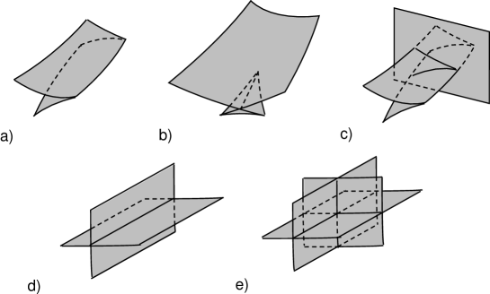
Figure 5. Generic Singularities for Legendrian projections of Legendrian surfaces: a) cuspidal edge, b) swallowtail, c) transverse intersection of cuspidal edge and smooth surface, d) transverse intersection of two smooth surfaces, and e) transverse intersection of three smooth surfaces.

Finally, we remark about the relation between the dual variety $M^{\vee}$ and the image $M_{\mathcal{L}}=\mathcal{L}(M)$ (or $M_{\tilde{\mathcal{L}}}=\tilde{\mathcal{L}}(M)$). To do so, we introduce a mapping involving ${\mathbb{R}}P^{n\,\vee}$ and $\tilde{\mathcal{T}}^{n}$. In ${\mathbb{R}}P^{n\,\vee}$, there is the distinguished point $\infty=<(0,\dots,0,1)>$. On ${\mathbb{R}}P^{n\,\vee}\backslash\{\infty\}$, we may take a point $<(y_{1},\dots,y_{n},y_{n+1})>$, and normalize it by

$$(y_{1}^{\prime},\dots,y_{n}^{\prime},y_{n+1}^{\prime})=c\cdot(y_{1},\dots,y_{n},y_{n+1}),\quad\mbox{where }\,c=(\sum_{i=1}^{n}y_{i}^{2})^{-\frac{1}{2}}.$$

Then, $\mathbf{n}_{y}=(y_{1}^{\prime},\dots,y_{n}^{\prime})$ is a unit vector. We then define a map $\nu:{\mathbb{R}}P^{n\,\vee}\backslash\{\infty\}\to\tilde{\mathcal{T}}^{n}$ sending $<(y_{1},\dots,y_{n},y_{n+1})>$ to $(\mathbf{n}_{y},y_{n+1}^{\prime}\boldsymbol{\epsilon})$. This is only well-defined up to multiplication by $-1$, which is why we must take the equivalence class in the pair of points. If we are on a region of ${\mathbb{R}}P^{n\,\vee}\backslash\{\infty\}$ where we can smoothly choose a direction for each line corresponding to a point in ${\mathbb{R}}P^{n\,\vee}$, then as for the case of the Lorentzian mapping, we can give a well-defined map to $\mathcal{T}^{n}$. This will be so when we consider $M^{\vee}$ for the oriented case. In such a situation, when the smooth hypersurface $M$ has a smooth unit normal vector field $\mathbf{n}$, it provides a positive direction in the line of linear forms vanishing on $T_{x}M$.

Then, we have the following relations.

Lemma 7.1.

The smooth mapping $\tilde{\nu}:{\mathbb{R}}P^{n\,\vee}\backslash\{\infty\}\to\tilde{\mathcal{T}}^{n}$ is a diffeomorphism.

Second, there is the relation between the duality map $\delta$ and the Lorentz map $\tilde{\mathcal{L}}$ (or $\mathcal{L}$).

Lemma 7.2.

If $M\subset{\mathbb{R}}^{n}$ is a smooth hypersurface, then the diagram (7.2) commutes, i.e. $\tilde{\nu}\circ\delta=\tilde{\mathcal{L}}$. If, in addition, $M$ has a smooth unit normal vector field $\mathbf{n}$, then there is the oriented version of diagram (7.2), $\nu\circ\delta=\mathcal{L}$.

$$M \overset{\delta}{\longrightarrow} {\mathbb{R}}P^{n\,\vee}$$

$$\underset{\tilde{\mathcal{L}}\,\,}{\searrow} \downarrow\tilde{\nu}$$

$$\tilde{\mathcal{T}}^{n}$$

As a consequence of these Lemmas and our earlier discussion about the singularities of $M^{\vee}$, we conclude that $M_{\tilde{\mathcal{L}}}$ (or $M_{\mathcal{L}}$) have the same singularities. Thus, we may suppose they are generic Legendrian singularities.

Remark 7.3.

Although by Lemma 7.1 ${\mathbb{R}}P^{n\,\vee}\backslash\{\infty\}$ is diffeomorphic to $\tilde{\mathcal{T}}^{n}$, the first space has a natural Riemannian structure while on $\tilde{\mathcal{T}}^{n}$ we have a Lorentzian metric. Hence, $\tilde{\nu}$ is not an isometry and does not map geodesics to geodesics.

Proof of Lemma 7.1.

There is a natural inverse to $\tilde{\nu}$ defined as follows: If $z=(\mathbf{n},c\boldsymbol{\epsilon})$ and $\mathbf{n}=(a_{1},\dots,a_{n})$, then we map $z$ to $<(a_{1},\dots,a_{n},-c)>$. We note that replacing $z$ by $-z$ does not change the line $<(a_{1},\dots,a_{n},-c)>$. This gives a well-defined smooth map $\tilde{\mathcal{T}}^{n}\to{\mathbb{R}}P^{n\,\vee}\backslash\{\infty\}$ which is easily checked to be the inverse of $\tilde{\nu}$. ∎

Proof of Lemma 7.2.

If $T_{x}M$ is defined by $\mathbf{n}\cdot\mathbf{x}=c$ with $\mathbf{n}=(a_{1},\dots,a_{n})$, then $\delta(x)=<(a_{1},\dots,a_{n},-c)>$. Then, as $\|\mathbf{n}\|=1$, $\tilde{\nu}(<(a_{1},\dots,a_{n},-c)>)=(a_{1},\dots,a_{n},c,c)=(\mathbf{n},c\boldsymbol{\epsilon})$, which is exactly $\mathcal{L}(x)$. ∎

Inverses of the Dual Variety and Lorentzian Mappings

We consider how to invert both $\delta$ and $\tilde{\mathcal{L}}$. We earlier remarked that in the complex algebraic setting, the inverse to $\delta$ is again a dual map $\delta^{\vee}$. As $\tilde{\nu}$ is a diffeomorphism, and diagram 7.2 commutes, inverting $\delta$ is equivalent to inverting $\tilde{\mathcal{L}}$. Also, constructing an inverse is a local problem, so we may as well consider the oriented case.

Proposition 7.4.

Let $M\subset{\mathbb{R}}^{n}$ be a generic smooth hypersurface with a smooth unit normal vector field $\mathbf{n}$. Suppose that the image $M_{\mathcal{L}}$ under $\mathcal{L}$ is a smooth submanifold of $\mathcal{T}^{n}$. Then, $M$ is obtained as the envelope of the collection of hyperplanes defined by $\mathbf{n}\cdot\mathbf{x}=c$ for $\mathcal{L}(x)=(\mathbf{n},c\boldsymbol{\epsilon})$.

Proof of Proposition 7.4.

We consider an $(n-1)$-dimensional submanifold of $\mathcal{T}^{n}$ parametrized by $u\in U$ given by $(\mathbf{n}(u),c(u)\boldsymbol{\epsilon})$. The collection of hyperplanes are given by $\Pi_{u}$ defined by $F(\mathbf{x},u)=\mathbf{n}(u)\cdot\mathbf{x}-c(u)=0$. Then, the envelope is defined by the collection of equations $F_{u_{i}}=0,i=1,\dots,n-1$ and $F=0$. This is the system of linear equations

(7.2) $$i)\,\,\,\mathbf{n}(u)\cdot\mathbf{x}=c(u)\qquad\mbox{and }\,ii)\,\,\,\mathbf{n}_{u_{i}}(u)\cdot\mathbf{x}=c_{u_{i}}(u),\,\,i=1,\dots,n-1$$

A sufficient condition that there exist for a given $u$ a unique solution to the system of linear equations in $\mathbf{x}$ is that the vectors $\mathbf{n},\mathbf{n}_{u_{1}},\dots,\mathbf{n}_{u_{n-1}}$ are linearly independent. Since $\mathbf{n}_{u_{i}}=-S(\dfrac{\partial}{\partial u_{i}})$, for $S$ the shape operator for $M$, linear independence is equivalent to $S$ not having any $0$-eigenvalues. Thus, $\mathbf{x}$ is not a parabolic point of $M$. For generic $M$, the set of parabolic points is a stratified set of codimension $1$ in $M$. Thus, off the image of this set, there is a unique point in the envelope.

Also, if we differentiate equation (7.2)-i) with respect to $u_{i}$ we obtain

(7.3) $$\mathbf{n}_{u_{i}}(u)\cdot\mathbf{x}\,+\,\mathbf{n}(u)\cdot\mathbf{x}_{u_{i}}\,\,=\,\,c_{u_{i}}(u)$$

Combining this with (7.2)-ii), we obtain

(7.4) $$\mathbf{n}(u)\cdot\mathbf{x}_{u_{i}}\,\,=\,\,0,$$

and conversely, (7.4) for $i=1,\dots,n-1$ and (7.3) imply (7.2)-ii). Thus, if we choose a local parametrization of $M$ given by $\mathbf{x}(u)$, then as $\mathbf{x}(u)$ is a point in its tangent space, it satisfies (7.2)-i), and hence (7.3), and also $\mathbf{n}$ being a normal vector field implies that (7.4) is satisfied for all $i$. Thus, (7.2)-ii) is satisfied. Hence, $M$ is part of the envelope. Also, for generic points of $M$, by the implicit function theorem, the set of solutions of (7.2) is locally a submanifold of dimension $n-1$. Hence, in a neighborhood of these generic points of $M$, the envelope is exactly $M$. Hence, the closure of this set is all of $M$ and still consists of solutions of (7.2). Thus, we recover $M$.

Second, to see that the equations (7.2) describe the inverse of the dual mapping, we note by Lemmas 7.1 and 7.1 that $\tilde{\nu}$ is a diffeomorphism, $\delta^{-1}=\tilde{\mathcal{L}}^{-1}\circ\tilde{\nu}$, and the preceding argument gives the local inverse to $\tilde{\mathcal{L}}$. ∎

8. Sufficient Condition for Smoothness of Envelopes

To describe the induced “geodesic flow”between hypersurfaces $M_{0}$ and $M_{1}$ in ${\mathbb{R}}^{n}$, we will use the Lorentzian geodesic flow in $\mathcal{T}^{n}$ and then find the corresponding flow by applying an inverse to $\mathcal{L}$. We begin by constructing the inverse for a $(n-1)$-dimensional manifold in $\mathcal{T}^{n}$ parametrized by $(\mathbf{n}(u),c(u)\boldsymbol{\epsilon})$, where $u=(u_{1},\dots,u_{n-1})$. We determine when the associated family of hyperplanes $\Pi_{u}=\{\mathbf{x}\in{\mathbb{R}}^{n}:\mathbf{n}(u)\cdot\mathbf{x}=c(u)\}$ has as an envelope a smooth hypersurface in ${\mathbb{R}}^{n}$.

We introduce a family of vectors in ${\mathbb{R}}^{n+1}$ given by $\tilde{\mathbf{n}}(u)=(\mathbf{n}(u),-c(u))$. We also denote $\dfrac{\partial\tilde{\mathbf{n}}}{\partial u_{i}}$ by $\tilde{\mathbf{n}}_{u_{i}}$. Next we consider the $n$-fold cross product in ${\mathbb{R}}^{n+1}$, denoted by $v_{1}\times v_{2}\times\cdots\times v_{n}$, which is the vector in ${\mathbb{R}}^{n+1}$ whose $i$-th coordinate is $(-1)^{i+1}$ times the $n\times n$ determinant obtained from the entries of $v_{1},\dots,v_{n}$ by removing the $i$-th entries of each $v_{j}$. Then, for any other vector $v$,

$$v\cdot(v_{1}\times v_{2}\times\cdots\times v_{n})\,\,=\,\,\det(v,v_{1},\dots,v_{n})$$

We let

$$\tilde{\mathbf{h}}\,\,=\,\,\tilde{\mathbf{n}}\times\tilde{\mathbf{n}}_{u_{1}}\times\cdots\times\tilde{\mathbf{n}}_{u_{n-1}}$$

We let $H(\tilde{\mathbf{n}})$ denote the $(n-1)\times(n-1)$ matrix of vectors $\tilde{\mathbf{n}}_{u_{i}\,u_{j}}$. Then we can form $H(\tilde{\mathbf{n}})\cdot\tilde{\mathbf{h}}$ to be the $(n-1)\times(n-1)$ matrix with entries $\tilde{\mathbf{n}}_{u_{i}\,u_{j}}\cdot\tilde{\mathbf{h}}$. Then, there is the following determination of the properties of the envelope of $\{\Pi_{u}\}$.

Proposition 8.1.

Suppose we have an $(n-1)$-dimensional manifold in $\mathcal{T}^{n}$ parametrized by $(\mathbf{n}(u),c(u)\boldsymbol{\epsilon})$, where $u=(u_{1},\dots,u_{n-1})$. We let $\{\Pi_{u}\}$ denote the associated family of hyperplanes. Then, the envelope of $\{\Pi_{u}\}$ has the following properties.

• There is a unique point $\mathbf{x}_{0}$ on the envelope corresponding to $u_{0}$ provided $\mathbf{n}(u_{0}),\mathbf{n}_{u_{1}}(u_{0}),\dots,\mathbf{n}_{u_{n-1}}(u_{0})$ are linearly independent. Then, the point is the solution of the system of equations (7.2).

• Provided i) holds, the envelope is smooth at $\mathbf{x}_{0}$ provided $H(\tilde{\mathbf{n}})\cdot\tilde{\mathbf{h}}$ is nonsingular for $u=u_{0}$.

• Provided ii) holds, the normal to the surface at $\mathbf{x}_{0}$ is $\mathbf{n}(u_{0})$ and $\Pi_{u_{0}}$ is the tangent plane at $\mathbf{x}_{0}$.

Proof of Proposition 8.1.

We use the line of reasoning for Proposition 7.4. the condition that a point $\mathbf{x}_{0}$ belong to the envelope of $\{\Pi_{u}\}$ is that it satisfy the system of equations (7.2). A sufficient condition that these equations have a unique solution for $u=u_{0}$ is exactly that $\mathbf{n}(u_{0}),\mathbf{n}_{u_{1}}(u_{0}),\dots,\mathbf{n}_{u_{n-1}}(u_{0})$ are linearly independent.

Furthermore, if this is true at $u_{0}$ then it is true in a neighborhood of $u_{0}$. Thus, we have a unique smooth mapping $\mathbf{x}(u)$ from a neighborhood of $u_{0}$ to ${\mathbb{R}}^{n}$. By the argument used to deduce (7.4), we also conclude

(8.1) $$\mathbf{n}(u)\cdot\mathbf{x}_{u_{i}}\,\,=\,\,0,\qquad i=1,\dots,n-1$$

Hence, if $\mathbf{x}(u)$ is nonsingular at $u_{0}$, then $\mathbf{n}(u_{0})$ is the normal vector to the envelope hypersurface at $\mathbf{x}_{0}$, so the tangent plane is $\Pi_{u_{0}}$. Thus iii) is true.

It remains to establish the criterion for smoothness in ii). As earlier mentioned the envelope in the neighborhood of a point $\mathbf{x}_{0}$ is the discriminant of the projection of $V=\{(\mathbf{x},u):F(\mathbf{x},u)=\mathbf{n}(u)\cdot\mathbf{x}-c(u)=0\}$ to ${\mathbb{R}}^{n}$. It is a standard classical result that at a point $(\mathbf{x}_{0},u_{0})\in V$, which projects to an envelope point $\mathbf{x}_{0}$, the envelope is smooth at $\mathbf{x}_{0}$ provided $(\mathbf{x}_{0},u_{0})$ is a regular point of $F$ (so $V$ is smooth in a neighborhood of $(\mathbf{x}_{0},u_{0})$) and the partial Hessian $(\dfrac{\partial^{2}F}{\partial u_{i}\,u_{j}}(\mathbf{x}_{0},u_{0}))$ is nonsingular. For our particular $F$ this Hessian becomes $H(\mathbf{n})\cdot\mathbf{x}_{0}-H(c)$, where $H(\mathbf{n})$ is the $(n-1)\times(n-1)$ matrix of vectors $(\mathbf{n}_{u_{i}\,u_{j}})$, and $H(\mathbf{n})\cdot\mathbf{x}_{0}$ denotes the $(n-1)\times(n-1)$ matrix whose entries are $\mathbf{n}_{u_{i}\,u_{j}}\cdot\mathbf{x}_{0}$. This can also be written $H(\tilde{\mathbf{n}})\cdot\tilde{\mathbf{x}}_{0}$, where $\tilde{\mathbf{x}}_{0}$ is the extension of $\mathbf{x}_{0}$ to ${\mathbb{R}}^{n+1}$ by adding $1$ as the $n+1$-st coordinate.

Now $\mathbf{x}_{0}$ is the unique solution of the system of linear equations (7.2). This solution is given by Cramer’s rule. Let $N(u_{0})$ denote the $n\times n$ matrix with columns $\mathbf{n}(u_{0}),\mathbf{n}_{u_{1}}(u_{0}),\dots,\mathbf{n}_{u_{n-1}}(u_{0})$. By Cramer’s rule, if we multiply $\tilde{\mathbf{x}}_{0}$ by $\det(N(u_{0}))$ we obtain $(-1)^{n}\tilde{\mathbf{h}}$. Thus, multiplying $H(\tilde{\mathbf{n}})\cdot\tilde{\mathbf{x}}_{0}$ by $\det(N(u_{0}))$ yields $(-1)^{n}H(\tilde{\mathbf{n}})\cdot\tilde{\mathbf{h}}$. Hence, the nonsingularity of $H(\tilde{\mathbf{n}})\cdot\tilde{\mathbf{h}}$ implies that of $(\dfrac{\partial^{2}F}{\partial u_{i}\,u_{j}}(\mathbf{x}_{0},u_{0}))$. ∎

Although Proposition 8.1 handles the case of a smooth manifold in $\mathcal{T}^{n}$, we saw in §7 that usually the image in $\mathcal{T}^{n}$ of a generic hypersurface $M$ in ${\mathbb{R}}^{n}$ will have Legendrian singularities and the image itself is a Whitney stratified set $\tilde{M}$. Next, we deduce the condition ensuring that the envelope is smooth at a singular point $\mathbf{x}_{0}$.

Because $\tilde{M}$ has Legendrian singularities, it has a special property. To expain it we use a special property which holds for certain Whitney stratified sets.

Definition 8.2.

An $m$-dimensional Whitney stratified set $M\subset{\mathbb{R}}^{k}$ has the Unique Limiting Tangent Space Property (ULT property) if for any $x\in M_{sing}$, a singular point of $M$, there is a unique $m$-plane $\Pi\subset{\mathbb{R}}^{k}$ such that for any sequence $\{x_{i}\}$ of smooth points in $M_{reg}$ such that $\lim x_{i}=x$, we have $\lim T_{x_{i}}M=\Pi$

Lemma 8.3.

For a generic Legendrian hypersurfaces $M\subset{\mathbb{R}}^{n}$, if $z\in\tilde{M}$, then $\tilde{M}$ can be locally represented in a neighborhood of $z$ as a finite transverse union of $(n-1)$-dimensional Whitney stratified sets $Y_{i}$ each having the ULT property.

Transverse union means that if $W_{ij}$ is the stratum of $Y_{i}$ containing $z$ than the $W_{ij}$ intersect transversally.

Proof.

The Lemma follows because $\tilde{M}$ consists of generic Legendrian singularities, which are either stable (or topologically stable) Legendrian singularities. These are either discriminants of stable unfoldings of multigerms of hypersurface singularities or transverse sections of such. Such discriminants are transverse unions of discriminants of individual hypersurface singularities, each of which have the ULT property by a result of Saito [Sa]. This continues to hold for transverse sections. ∎

We shall refer to these as the local components of $\tilde{M}$ in a neighborhood of $z$.

There is then a corollary of the preceding.

Corollary 8.4.

Suppose that $\tilde{M}$ is an $(n-1)$–dimensional Whitney stratified set in $\mathcal{T}^{n}$ such that: at every smooth point $z$ of $\tilde{M}$, the hypotheses of Proposition 8.1 holds; and at all singular points $\tilde{M}$ is locally the finite union of Whitney stratified sets $Y_{i}$ each having the ULT property. Then,

• The envelope of $M$ of $\tilde{M}$ has a unique point $x\in M$ for each $z\in\tilde{M}_{reg}$, and $M$ is smooth at all points corresponding to points in $\tilde{M}_{reg}$.

• At each singular point $z$ of $\tilde{M}$, there is a point in $M$ corresponding to each local component of $\tilde{M}$ in a neighborhood of $z$.

Proof.

First, if $z\in\tilde{M}_{reg}$ and satisfies the conditions of Proposition 8.1, then there is a unique envelope point corresponding to $z$ and the envelope is smooth at that point.

Second, via the isomorphism $\tilde{\nu}$ and the commutative diagram (3.1), the envelope construction corresponds to the inverse $\delta^{\vee}$ of $\delta$ (or rather a local version since we have an orientation). Under the isomorphism $\tilde{\nu}$, for each point $z\in\tilde{M}_{sing}$ there corresponds a unique point in the envelope for each local component of $\tilde{M}$ containing $z$. It is obtained as $\delta^{\vee}$ applied to the unique limiting tangent space of $z$ associated to the local component in $\tilde{M}_{reg}$. ∎

9. Induced Geodesic Flow between Hypersurfaces

We can bring together the results of the previous sections to define the Lorentzian geodesic flow between two smooth generic hypersurfaces with a correspondence. We denote our hypersurfaces by $M_{0}$ and $M_{1}$ and let $\chi:M_{0}\to M_{1}$ be a diffeomorphism giving the correspondence. Note that we allow the hypersurfaces to have boundaries.

We suppose that both are oriented with unit normal vector fields $\mathbf{n}_{0}$ and $\mathbf{n}_{1}$. We also need to know that they have a “local relative orientation”.

Definition 9.1.

We say that the oriented manifolds $M_{0}$ and $M_{1}$, with unit normal vector fields $\mathbf{n}_{0}$ and $\mathbf{n}_{1}$, and with correspondence $\chi:M_{0}\to M_{1}$ are relatively oriented if there is a smooth function $\theta(x):M_{0}\to(-\pi,\pi)$ such that $\mathbf{n}_{0}(x)\cdot\mathbf{n}_{1}(\chi(x))=\theta(x)$ for all $x\in M_{0}$.

An example of a Lorentzian geodesic flow between curves in ${\mathbb{R}}^{2}$ is illustrated in Figure 6.

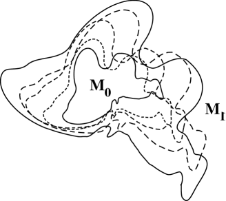
Figure 6. A nonsingular Lorentzian Geodesic Flow between the curve $M_{0}$ in ${\mathbb{R}}^{2}$ and the curve $M_{1}$, which was obtained from $M_{0}$ via a composition of a rigid motion and a homothety. The correspondence is given by the combined transformations, and then the relative orientation is a constant angle. As remarked in b) of Figure 2 there does not exist a nonsingular geodesic flow between $M_{0}$ and $M_{1}$ in ${\mathbb{R}}^{2}$.

If the preceding example in Figure 6 is slightly perturbed, then the existence of a nonsingular Lorentzian flow is guaranteed by the next theorem.

Theorem 9.2 ( Existence, Smooth Dependence and Stability of Lorentzian Geodesic Flows ).

Suppose smooth generic hypersurfaces $M_{0}$ and $M_{1}$ are oriented by smooth unit normal vector fields $\mathbf{n}_{i},i=0,1$ and are relatively oriented by $\theta$ for the diffeomorphism $\chi:M_{0}\to M_{1}$.

1. (Existence and Smoothness:) Then for the given relative orientation, is a smooth Lorentzian geodesic flow $\psi_{t}:M_{0}\times[0,1]\to\mathcal{T}^{n}$ between $M_{0}$ and $M_{1}$ given by (9.1).

2. (Stability:) There is a neighborhood $\mathcal{U}$ of $\chi$ in ${\rm Diff}\,(M_{0},M_{1})$ (for the $C^{\infty}$–topology) such that if $\chi^{\prime}\in\mathcal{U}$, then $M_{0}$ and $M_{1}$ are relatively oriented for $\chi^{\prime}$ and the map $\Psi:\mathcal{U}\to C^{\infty}(M_{0}\times[0,1],\mathcal{T}^{n})$ mapping $\chi^{\prime}$ to the associated Lorentzian flow $\tilde{\psi}^{\prime}_{t}$ is continuous.

3. (Smooth Dependence:) Let $\chi_{s}:M_{0\,s}\to M_{1\,s}$ be a smooth family of diffeomorphisms between smooth families of hypersurfaces for $s\in S$, a smooth manifold (i.e. $M_{i\,s}$ is the image of $M_{i}\times S$ under a smooth family of embeddings) so that $M_{0\,s}$ and $M_{1\,s}$ are relatively oriented for $\chi_{s}$ for each $s$ by a smooth map $\theta(x,s):M_{0\,s}\to(-\pi,\pi)$ in $(x,s)$. Then, the family of Lorentzian Geodesic flows $\tilde{\psi}_{s,t}:M_{0}\times S\times[0,1]\to\mathcal{T}^{n}$ between $M_{0\,s}$ and $M_{1\,s}$ is a smooth function of $(x,s,t)$.

Proof.

Using the form of the Lorentzian geodesic flow given by Proposition 4.1 we have the Lorentzian geodesic flow is defined by

(9.1) $$\psi_{t}(x)\quad=\quad\lambda(t,\theta(x))\,z_{1}(x)\,+\,\lambda(1-t,\theta(x))\,z_{0}(x)\qquad\mbox{for }0\leq t\leq 1$$

Here $z_{0}(x)=(\mathbf{n}_{0}(x),c_{0}(x))$ for $T_{x}M_{0}$ defined by $\mathbf{n}_{0}(x)\cdot\mathbf{x}=c_{0}(x)$, and $z_{1}(x)=(\mathbf{n}_{1}(x),c_{1}(x))$ for $T_{\chi(x)}M_{1}$ defined by $\mathbf{n}_{1}(x)\cdot\mathbf{x}=c_{1}(x)$. As $z_{i}(x)$ and $\theta(x)$ depend smoothly on $x\in M$ and $\lambda(t,\theta)$ is smooth on $[0,1]\times(-\pi,\pi)$, $\psi_{t}(x)$ is smooth in $(x,t)$. Hence, the Lorentzian flow is a smooth well-defined flow between $(\mathbf{n}_{0}(x),c_{0}(x)\boldsymbol{\epsilon})$ and $(\mathbf{n}_{1}(\chi(x)),c_{1}(\chi(x))\boldsymbol{\epsilon})$

For smooth dependence 3), we use an analogous argument. We use (9.1) but with $\theta(x)$ replaced by $\theta(x,s)$ and each $z_{i}(x)$ by $z_{i}(x,s)=(\mathbf{n}_{1}(x,s),c_{1}(x,s))$ where $T_{x}M_{0\,s}$ is defined by $\mathbf{n}_{0}(x,s)\cdot\mathbf{x}=c_{0}(x,s)$ and $T_{\chi(x,s)}M_{1\,s}$ is defined by $\mathbf{n}_{1}(x,s)\cdot\mathbf{x}=c_{1}(x,s)$.

Finally to establish the stability, given $\chi$ for which $M_{0}$ and $M_{1}$ are relatively oriented via the smooth function $\theta(x)$, we let $\delta(x)$ be a smooth nonvanishing function such that $\delta(x)<1/3(\pi-\theta(x))$ and $\lim\delta(x)=0$ as $x$ approaches any “unbounded boundary component at $\infty$”  of $M_{0}$. Then, as $(-\pi,\pi)$ is contractible there is a Whitney open neighborhood $\mathcal{U}$ of $\chi$ such that if $\chi^{\prime}\in\mathcal{U}$ then there is a smooth $\theta^{\prime}:M_{0}\to(-\pi,\pi)$ such that $\mathbf{n}_{0}(x)\cdot\mathbf{n}_{1}(\chi^{\prime}(x))=\cos(\theta^{\prime}(x))$ and $|\theta^{\prime}(x)-\theta(x)|<\delta(x)$ for all $x\in M_{0}$. Furthermore, $\theta^{\prime}$ depends continuously on $\chi^{\prime}$. Thus, the corresponding flow in (9.1) defined by $\theta^{\prime}$ depends continuously on $\chi^{\prime}$.

Specifically, given $\chi^{\prime}\in\mathcal{U}$, consider the mapping $\chi^{\prime}_{\mathcal{L}}:M_{0}\to\mathcal{T}^{n}\times\mathcal{T}^{n}$ defined by $x\mapsto((\mathbf{n}_{0}(x),c_{0}(x)),(\mathbf{n}_{1}(x),c_{1}(x)))$, where $(\mathbf{n}_{0}(x),c_{0}(x))$ defines the tangent space $T_{x}M_{0}$ and $(\mathbf{n}_{1}(x),c_{1}(x))$ defines the tangent space $T_{\chi^{\prime}(x)}M_{1}$. Then, $\chi^{\prime}_{\mathcal{L}}$ is defined using the first derivatives of the embeddings $M_{i}\subset{\mathbb{R}}^{n}$ and $\chi^{\prime}$ composed with algebraic operations. Each such operation is continous in the Whitney $C^{\infty}$–topology and so defines a continuous map $\mathcal{L}^{\prime}:\mathcal{U}\to C^{\infty}(M_{0},\mathcal{T}^{n}\times\mathcal{T}^{n})$. Lastly, the Lorentzian flow $\psi_{t}$ is defined by (4.4), and is the composition of $\mathcal{L}^{\prime}$ with algebraic operations involving the smooth functions $\lambda(x,\theta)$, and is again continuous in the $C^{\infty}$–topology. Hence, the combined composition mapping $\chi{\prime}\to\psi_{t}$ is continuous in the $C^{\infty}$–topology.

∎

Remark .

We note there are two consequences of 2) of Theorem 9.2. First, $M_{0}$ and $M_{1}$ may remain fixed, but the correspondence $\chi$ varies in a family. Then the corresponding Lorentzian geodesic flows vary in a family. Second, $M_{0}$ and $M_{1}$ may vary in a family with a corresponding varying correspondence, then the Lorentzian geodesic flow will also vary smoothly in a family.

Nonsingularity of Level Hypersurfaces of Lorentzian Geodesic Flows in ${\mathbb{R}}^{n}$

It remains to determine when the corresponding Lorentzian geodesic flows in ${\mathbb{R}}^{n}$ will have analogous properties. We give a criterion involving a generalized eigenvalue for a pair of matrices.

We consider the vector fields on $M_{0}$, $\mathbf{n}_{0}(x)$ and $\mathbf{n}_{1}(\chi(x))$. For any vector field $\mathbf{n}(x)$ on $M_{0}$ with values in ${\mathbb{R}}^{n}$, we let $N(x)=(\mathbf{n}(x)\,|\,d\mathbf{n}(x))$ be the $n\times n$ matrix with columns $\mathbf{n}(x)$ viewed as a column vector and $d\mathbf{n}(x)$ the $n\times(n-1)$ Jacobian matrix. If we have a local parametrization $\mathbf{x}(u)$ of $M_{0}$, then we may represent the vector field $\mathbf{n}$ as a function of $u$, $\mathbf{n}(u)$. Then, $N(\mathbf{x}(u))$ is the $n\times n$ matrix with columns $\mathbf{n}(u),\mathbf{n}_{u_{1}}(u),\dots,\mathbf{n}_{u_{n-1}}(u)$. We denote this matrix for $\mathbf{n}_{0}$ by $N_{0}(x)$, and that for $\mathbf{n}_{1}(\chi(x))$ by $N_{1}(x)$ (or $N_{0}(u)$ and $N_{1}(\chi(u))$ if we have parametrized $M_{0}$). By i) of Proposition 8.1 the Lorentzian geodesic flow in ${\mathbb{R}}^{n}$ will be well-defined provided the corresponding matrix $N_{t}(x)$ is nonsingular at all points of the flow $\tilde{\psi}_{t}(x)$. We determine this by decomposing $N_{t}(x)$ into two parts.

First, there is the parametrized family of $n\times n$–matrices

(9.2) $$\widetilde{N}_{t}(x)\,\,\overset{def}{=}\,\,\lambda(t,\theta)\,N_{1}(x)\,+\,\lambda(1-t,\theta)\,N_{0}(x)$$

This captures the change resulting from the change in $x$. To also capture the change resulting from that in $\theta$, we introduce a second matrix $\dfrac{\partial\theta}{\partial\mathbf{u}}\,\mathbf{n}_{0}$ whose first column equals the vector $0$ and whose $j+1$–th column is the vector $\dfrac{\partial\theta}{\partial u_{j}}\,\mathbf{n}_{0}$, for $j=1,\dots,n-1$. Then, the nonsingularity criterion will be based on whether the pair of matrices $(\tilde{N}_{t}(x),\dfrac{\partial\theta}{\partial\mathbf{u}}\,\mathbf{n}_{0})$ does not have a specific generalized eigenvalue.

Specifically we introduce one more function.

$$\sigma(x,\theta)\,\,=\,\,\dfrac{\partial\lambda}{\partial\theta}(x,\theta)-x\cot(\theta)\lambda(x,\theta)$$

Then, we compute for $\theta\neq 0$

(9.3) $$\dfrac{\partial\lambda(x,\theta)}{\partial\theta}\,\,=\,\,\frac{x\,\sin(\theta)\cos(x\theta)\,-\,\sin(x\theta)\cos\theta}{\sin^{2}\theta}$$

and $\dfrac{\partial\lambda(x,\theta)}{\partial\theta}_{|\theta=0}=0$. Using (9.3), a direct calculation shows for all $0\leq x\leq 1$.

$$\sigma(x,\theta)\,\,=\,\,\frac{\cos((1-x)\theta)\sin(x\theta)\,-\,x\,\sin\theta}{\sin(x\theta)\,\sin\theta}\,\,=\,\,\frac{\cos((1-x)\theta)}{\sin\theta}\,-\,\frac{x}{\sin(x\theta)}$$

if $0<|\theta|<\pi$; and

$$\sigma(x,0)\,\,=\,\,0$$

We also define

(9.4) $$N_{t}^{\prime}(x)\,\,\overset{def}{=}\,\,\tilde{N}_{t}(x)\,+\,\sigma(t,\theta)\,\dfrac{\partial\theta}{\partial\mathbf{u}}\,\mathbf{n}_{0}$$

Then, for any pair $(x,t)$, $N_{t}^{\prime}(x)$ is singular iff $-\sigma(t,\theta(x))$ is a generalized eigenvalue for $(\tilde{N}_{t}(x),\dfrac{\partial\theta}{\partial\mathbf{u}}\,\mathbf{n}_{0})$.

Consider the Lorentzian geodesic flow $\tilde{\psi}_{t}(x)=(\mathbf{n}_{t}(x),c_{t}(x)\boldsymbol{\epsilon})$ between $\mathcal{L}(x)=(\mathbf{n}_{0}(x),c_{0}(x)\boldsymbol{\epsilon})$ and $\mathcal{L}(\chi(x))=(\mathbf{n}_{1}(\chi(x)),c_{1}(\chi(x))\boldsymbol{\epsilon})$ for all $x\in M_{0}$. We let $\tilde{M}_{t}=\tilde{\psi}_{t}(M_{0})$, and we let $M_{t}$ denote the envelope of $\tilde{M}_{t}$.

Then there are the following properties for the envelopes $M_{t}$ of the flow for all time $0\leq t\leq 1$.

Theorem 9.3.

Suppose smooth generic hypersurfaces $M_{0}$ and $M_{1}$ are oriented by smooth unit normal vector fields $\mathbf{n}_{i},i=0,1$ and are relatively oriented by $\theta(u)$. Let $\tilde{\psi}_{t}$ be the Lorentzian geodesic flow between $\tilde{M}_{0}$ and $\tilde{M}_{1}$ which is smooth. If $M_{t}$ is the family of envelopes obtained from the flow $\tilde{M}_{t}=\tilde{\psi}_{t}(\tilde{M}_{0})$, then suppose that for each time $t$, $\tilde{M}_{t}$ has only generic Legendrian singularities as in §7 (as e.g. in Fig. 5). Then,

1. $M_{t}$ will have a unique point corresponding to $z=\tilde{\psi}_{t}(x)\in\tilde{M}_{t}$ provided (9.4) is nonsingular.

2. The envelope $M_{t}$ will be smooth at points corresponding to a smooth point $z\in\tilde{M}_{t}$ satisfying (9.4) provided $H(\tilde{\mathbf{n}}_{t}(x))\cdot\tilde{\mathbf{h}}_{t}(x)$ is nonsingular. Here $\tilde{\mathbf{h}}_{t}(x)$ is defined from $\tilde{\mathbf{n}}_{t}(x)$ as in §8.

3. At points corresponding to singular points $z\in\tilde{M}_{t}$, there is a unique point on $M_{t}$ for each local component of $\tilde{M}$ in a neighborhood of $z$. This point is the unique limit of the envelope points corresponding to smooth points of the component of $\tilde{M}_{t}$ approaching $z$.

Remark 9.4.

We observe that as a result of Theorem 9.3, we can remark about the uniqueness of the resulting geodesic flow from non-parabolic points of $M_{0}$. Then, $N_{0}(u)$ is non singular for each non-parabolic point $\mathbf{x}(u)$. If $N_{1}(\chi(u))$ is sufficiently close to $N_{0}(u)$ then $\widetilde{N}_{t}(u)$ will be nonsingular. This is given by a $C^{1}$-condition on the normal vector fields to the surfaces. If in addition, $\theta(u)$, the angle between $\mathbf{n}_{0}(u)$ and $\mathbf{n}_{1}(\chi(u))$, has small variation as a function of $u$, then the term $\sigma(t,\theta)\,\dfrac{\partial\theta}{\partial\mathbf{u}}$ will be small in the $C^{0}$ sense. Thus, if it is sufficiently small, then together with the $C^{1}$ closeness of (nonsingular) $N_{0}(u)$ and $N_{1}(\chi(u))$ implies that $N_{t}^{\prime}(u)$ is nonsingular. Hence, by i) of Theorem 9.3 the flow is uniqely defined. Together these are $C^{2}$ conditions on $N_{0}(u)$ and $N_{1}(\chi(u))$.

Proof of Theorem 9.3 .

For 2), given that 1) holds, we may apply ii) of Proposition 8.1. For 3) we may apply Corollary 8.4. To prove 1), we will apply i) of Proposition 8.1. We must give a sufficient condition that $N_{t}(x)$ is nonsingular for $0\leq t\leq 1$. We choose local coordinates $u$ for a neighborhood of $\mathbf{x}_{0}$. For a geodesic $(\mathbf{n}_{t}(u),c_{t}(u)\boldsymbol{\epsilon})$ between $(\mathbf{n}_{0}(u),c_{0}(u)\boldsymbol{\epsilon})$ and $(\mathbf{n}_{1}(u),c_{1}(u)\boldsymbol{\epsilon})$ given by (4.4), we must compute $\mathbf{n}_{t\,u_{i}}(u)$. We note that not only $\mathbf{n}_{i},i=1,2$ but also $\theta$ depends on $u$. We obtain

(9.5) $$\mathbf{n}_{t\,u_{i}}\,\,=\,\,\lambda(t,\theta)\,\mathbf{n}_{1\,u_{i}}\,+\,\lambda(1-t,\theta)\,\mathbf{n}_{0\,u_{i}}\,+\,\dfrac{\partial\lambda(t,\theta)}{\partial u_{i}}\,\mathbf{n}_{1}\,+\,\dfrac{\partial\lambda(1-t,\theta)}{\partial u_{i}}\,\mathbf{n}_{0}$$

Then, $\dfrac{\partial\lambda(t,\theta)}{\partial u_{i}}=\dfrac{\partial\theta}{\partial u_{i}}\,\dfrac{\partial\lambda(t,\theta)}{\partial\theta}$. Applying (9.3) with $x=t$ and $1-t$, we obtain for the last two terms on the RHS of (9.5)

(9.6) $$\dfrac{\partial\lambda(t,\theta)}{\partial u_{i}}\,\mathbf{n}_{1}\,+\,\dfrac{\partial\lambda(1-t,\theta)}{\partial u_{i}}\,\mathbf{n}_{0}\,\,=\,\,\dfrac{\partial\theta}{\partial u_{i}}\big{(}\frac{t\,\cos(t\,\theta)}{\sin\theta}\mathbf{n}_{1}\,+\,\frac{(1-t)\,\cos((1-t)\,\theta)}{\sin\theta}\mathbf{n}_{0}\\ \qquad-\cot\theta\,(\lambda(t,\theta)\,\mathbf{n}_{1}\,+\,\lambda(1-t,\theta)\,\mathbf{n}_{0})\big{)}$$

We see that the last expression in (9.6) is a multiple of $\mathbf{n}_{t}$. We can subtract a multiple of $\mathbf{n}_{t}$ from $\mathbf{n}_{t\,u_{i}}$ without altering the rank of the matrix $N_{t}$. Then, after subtracting $\dfrac{\partial\theta}{\partial u_{i}}\,\cot\theta\,\mathbf{n}_{t}$ from the RHS of (9.6), we obtain

(9.7) $$\dfrac{\partial\theta}{\partial u_{i}}\big{(}\frac{t\,\cos(t\,\theta)}{\sin\theta}\mathbf{n}_{1}\,+\,\frac{(1-t)\,\cos((1-t)\,\theta)}{\sin\theta}\mathbf{n}_{0}\big{)}$$

Then, in addition, we can subtract $\dfrac{\partial\theta}{\partial u_{i}}\,t\cot(t\,\theta)\,\mathbf{n}_{t}$ from the RHS of (9.7) so the term involving $\mathbf{n}_{1}$ is removed. We are left with

(9.8) $$\dfrac{\partial\theta}{\partial u_{i}}\,\big{(}\frac{(1-t)\,\cos((1-t)\,\theta)}{\sin\theta}\,-\,t\,\cot(t\theta)\,\frac{\sin((1-t)\theta)}{\sin\theta}\big{)}\,\mathbf{n}_{0}$$

Adding the two terms in the parentheses in (9.8), rearranging, and using the formula for $\sin(A+B)$, we obtain $\sigma(t,\theta)$, so that (9.8) becomes $\dfrac{\partial\theta}{\partial u_{i}}\,\sigma(t,\theta)\,\mathbf{n}_{0}$. Thus, applying the preceding to each $\mathbf{n}_{t\,u_{i}}$ we may replace each of them with

$$\lambda(t,\theta)\,\mathbf{n}_{1\,u_{i}}\,+\,\lambda(1-t,\theta)\,\mathbf{n}_{0\,u_{i}}\,+\,\dfrac{\partial\theta}{\partial u_{i}}\,\sigma(t,\theta)\,\mathbf{n}_{0}$$

without changing the rank. We conclude that $N_{t}$ has the same rank as the matrix $N_{t}^{\prime}$ given in (9.4).

It remains to consider the case when $\theta=0$. Then, both $\dfrac{\partial\lambda}{\partial\theta}(t,0)=0$ and $\dfrac{\partial\sigma}{\partial\theta}(t,0)=0$, so that the nonsingularity reduces to that for $\tilde{N}_{t}(x)$. ∎

Remark .

If $\mathbf{n}_{1}(\chi(x_{0}))\neq\mathbf{n}_{0}(x_{0})$, then there is a neighborhood $x_{0}\in W\subset M_{0}$ such that $\mathbf{n}_{1}(\chi(x))\neq\mathbf{n}_{0}(x)$ for $x\in W$. Then, there is a smooth unit tangent vector field $\mathbf{w}$ defined on $W$ such that $\mathbf{n}_{1}(\chi(x))$ lies in the vector space spanned by $\mathbf{n}_{0}(x)$ and $\mathbf{w}(x)$, and $\mathbf{n}_{1}(\chi(x))\cdot\mathbf{w}(x)\geq 0$ for all $x\in W$. Then, smoothness follows explicitly using the geodesics given in Proposition 4.1 by (4.4).

10. Results for the Case of Surfaces in ${\mathbb{R}}^{3}$

Now we consider the special case of surfaces $M_{i}\subset{\mathbb{R}}^{3}$, i = 1, 2 for which there is a correspondence given by the diffeomorphism $\chi:M_{0}\to M_{1}$. We suppose each $M_{i}$ is a generic smooth surface with $\mathbf{n}_{0}=(a_{1},a_{2},a_{3})$ and $\mathbf{n}_{1}=(a^{\prime}_{1},a^{\prime}_{2},a^{\prime}_{3})$ smooth unit normal vector fields on $M_{0}$, respectively $M_{1}$. We assume that $X(u_{1},u_{2})$ is a local parametrization of $M_{0}$. Each $a_{i}$ is a function of $(u_{1},u_{2})$ via the local parametrization $X(u_{1},u_{2})$. Likewise, each $a_{i}^{\prime}$ is a function of $(u_{1},u_{2})$ via the local parametrization $\chi\circ X(u_{1},u_{2})$ Also, let $\mathbf{n}_{i}(u)\cdot\mathbf{x}=c_{i}(u)$ define the tangent planes for $M_{0}$ at $X(u_{1},u_{2})$, respectively $M_{1}$ at $\chi(X(u_{1},u_{2}))$.

We let

$$\mathbf{n}_{t}\,\,=\,\,(a_{1\,t},a_{2\,t},a_{3\,t})\,\,=\,\,\lambda(t,\theta)\,(a^{\prime}_{1},a^{\prime}_{2},a^{\prime}_{3})\,+\,\lambda(1-t,\theta)\,(a_{1},a_{2},a_{3})$$

and $c_{t}(u)=\lambda(t,\theta)\,c_{1}\,+\,\lambda(1-t,\theta)\,c_{0}$. Then,

(10.1) $$N_{t}\,\,=\,\,\begin{pmatrix}a_{1\,t}&a_{1\,t,u_{1}}&a_{1\,t,u_{2}}\\ a_{2\,t}&a_{2\,t,u_{1}}&a_{2\,t,u_{2}}\\ a_{3\,t}&a_{3\,t,u_{1}}&a_{3\,t,u_{2}}\end{pmatrix}$$

Remark .

Note here and what follows we use the following notation. For quantities defined for a flow, we denote dependence on $t$ by a subscript. We also want to denote partial derivatives with respect to the parameters $u_{i}$ by a subscript. To distinguish them, the subscripts appearing after a comma will denote the partial derivatives. Hence, for example, in (10.1) $a_{i\,t,u_{j}}=\dfrac{\partial a_{i\,t}}{\partial u_{j}}$.

Existence of Envelope Points

The sufficient condition that there is a unique point $X_{t_{0}}(u)$ in the Lorentzian geodesic flow in ${\mathbb{R}}^{3}$ at time $t=t_{0}$ is that (10.1) evaluated at $t=t_{0}$ and $u=(u_{1},u_{2})$ is nonsingular. Then, the unique point is the solution of the linear system.

(10.2) $$N_{t_{0}}^{T}\cdot\mathbf{x}\,\,=\,\,\mathbf{c}$$

with $\mathbf{x}$ and $\mathbf{c}$ column matrices with entries $x_{1},x_{2},x_{3}$, respectively $c_{t_{0}},c_{t_{0},u_{1}},c_{t_{0},u_{2}}$, $a_{i\,t,u_{j}}=\dfrac{\partial a_{i\,t}}{\partial u_{j}}$, and $N_{t_{0}}$ is given by (10.1).

Furthermore, the nonsingularity of (10.1) is equivalent to that of (10.3).

(10.3) $$N^{\prime}_{t_{0}}\,\,=\,\,\lambda(t_{0},\theta)\,N_{1}\,+\,\lambda(1-t_{0},\theta)\,N_{0}+\sigma(t_{0},\theta)\,\dfrac{\partial\theta}{\partial\mathbf{u}}\,\mathbf{n}_{0}$$

where

(10.4) $$\dfrac{\partial\theta}{\partial\mathbf{u}}\,\mathbf{n}_{0}\,\,=\,\,\begin{pmatrix}0&\theta_{u_{1}}a_{1}&\theta_{u_{2}}a_{1}\\ 0&\theta_{u_{1}}a_{2}&\theta_{u_{2}}a_{2}\\ 0&\theta_{u_{1}}a_{3}&\theta_{u_{2}}a_{3}\end{pmatrix}$$

Smoothness of the Envelope

For the smoothness of $M_{t_{0}}$ at the point $X_{t_{0}}(u_{1},u_{2})$, we let

$$\tilde{\mathbf{n}}_{t_{0}}=(a_{1\,t_{0}},a_{2\,t_{0}},a_{3\,t_{0}},-c_{t_{0}})$$

evaluated at $u=(u_{1},u_{2})$. Also, we let $\tilde{\mathbf{h}}_{t_{0}}=\tilde{\mathbf{n}}_{t_{0}}\times\tilde{\mathbf{n}}_{t_{0}\,u_{1}}\times\tilde{\mathbf{n}}_{t_{0}\,u_{1}}$, which is the analogue of the cross product but for vectors in ${\mathbb{R}}^{4}$. It is the vector whose $j$–th entry is $(-1)^{j+1}$ times by taking the $3\times 3$ determinant of the submatrix obtained by deleting the $j$–th column of

(10.5) $$\begin{pmatrix}a_{1\,t_{0}}&a_{2\,t_{0}}&a_{3\,t_{0}}&-c_{t_{0}}\\ a_{1\,t_{0},u_{1}}&a_{2\,t_{0},u_{1}}&a_{3\,t_{0},u_{1}}&-c_{t_{0},u_{1}}\\ a_{1\,t_{0},u_{2}}&a_{2\,t_{0},u_{2}}&a_{3\,t_{0},u_{2}}&-c_{t_{0},u_{2}}\end{pmatrix}$$

Then, we form the $2\times 2$–matrix $H(\tilde{\mathbf{n}}_{t}(u))\cdot\tilde{\mathbf{h}}_{t})$ with $ij$–th entry $\mathbf{n}_{t,u_{i}u_{j}}(u)~{}\cdot~{}\tilde{\mathbf{h}}_{t}(u)$ for $u=(u_{1},u_{2})$. Then, from Theorem 9.3, we conclude that for a point uniquely defined by (10.2) the envelope is smooth at $X_{t_{0}}(u)$ if $H(\tilde{\mathbf{n}}_{t_{0}}(u))\cdot\tilde{\mathbf{h}}_{t_{0}}(u)$ is nonsingular.

Envelope Points corresponding to Legendrian Singular Points

Third, the generic Legendrian singularities for surfaces are those given in Fig. 5). For these:

1. At points on cuspidal edges or swallowtail points $z\in\tilde{M}_{t}$, there is a unique point on $M_{t}$ which is the unique limit of the envelope points corresponding to smooth points of $\tilde{M}_{t}$ approaching $z$.

2. At points $z\in\tilde{M}_{t}$ which are tranverse intersections of two or three smooth surfaces, or the transverse intersection of a smooth surface and a cuspidal edge, there is a unique point in $M_{t}$ for each smooth surface passing through $z$ (and one for the cuspidal edge).

Example 10.1.

As an example, we consider the Lorentzian geodesic flows between the surfaces $M_{1}$ given by $z=2-.2(x^{2}+y^{2})$, $M_{2}$ given by $z=.5-.05(x^{2}+y^{2})$, and $M_{3}$ given by $z=4-.5(x^{2}+y^{2})$. We consider two correspondences and the resulting Lorentzian geodesic flow between them. The first assigns to each point in $M_{1}$ the point in $M_{3}$ with the same coordinates $(x,y)$ so the points on the same vertical lines correspond. For the second, each point in $M_{2}$ corresponds to the point in $M_{3}$ in the same vertical line. For the third, we assign to each point $(x,y,z)$ of $M_{2}$ the point $(\frac{2}{5}x,\frac{2}{5}y,\frac{2}{5}z+3.2)$ in $M_{3}$.

Although for the first two there are simple Euclidean geodesic flows in ${\mathbb{R}}^{3}$ along the vertical lines, these are not the Lorentzian geodesic flow lines.

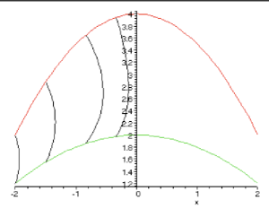
(a)                                         (b)

Figure 7. The Lorentzian geodesic flow between $M_{1}$ and $M_{3}$ viewed in a vertical plane through the $z$-axis. In a) are shown the nonsingular level surfaces of the flow and in b) the corresponding geodesic flow curves. The nonsingularity of flow is seen in b) with the geodesic flow curves not intersecting.

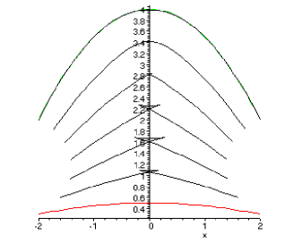
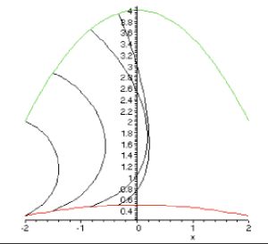
(a)                                     (b)

Figure 8. Comparison of Lorentzian geodesic flows between $M_{2}$ and $M_{3}$ in a vertical plane through the $z$-axis. In a) the level sets exhibit cusp singularity formation. In b) are shown the Lorentzian geodesic curves which intersect and produce the singularities.

For the third, $M_{3}$ is obtained from $M_{2}$ by a combination of the homothety of multiplication by $\frac{2}{5}$ combined with the translation by $(0,0,3.2)$. Hence, for the second case the Lorentzian geodesic flow is given by Corollary 5.4 to be along the lines joining the corresponding points and is given by

$$(x,y,z)\,\mapsto\,((1-\frac{3}{5}t)x,(1-\frac{3}{5}t)y,(1-\frac{3}{5}t)z+3.2t)\,.$$

By the circular symmetry of each surface about the $z$-axis, we may view the Lorentzian geodesics in a vertical plane through the $z$-axis. We may compute both the level sets of the Lorentzian geodesic flow and the corresponding geodesics using Proposition 8.1 and solving the systems of equations (7.2). We show the results of the computations using the software Maple in Figures 7 and 8. The Lorentzian geodesic flow between $M_{1}$ and $M_{3}$ with the vertical correspondence is nonsingular, as shown by the level sets and geodesic curves in Figure 7. By comparison, the Lorentzian geodesic flow between $M_{2}$ and $M_{3}$ for the vertical correspondence is singular. We see the cusp formation in the level sets in Figure 8 a). The singularities result from the intersection of the geodesics seen in and the individual flow curves in b). We also see that the increased bending of the geodesics versus those in Figure 7 result from the increases in the changes in tangent directions, leading to the formation of cusp singularities. By contrast, for the second correspondence resulting from the action of the element of the extended Poincare group, geodesics are straight lines as shown in Figure 9 and the flow is nonsingular.

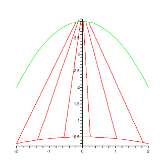
Figure 9. Lorentzian geodesic flow between $M_{2}$ and $M_{3}$ in a vertical plane through the $z$-axis for the correspondence arising from the action of an element of the extended Poincare group given by a homothety combined with a translation. The geodesics are straight lines and the flow is nonsingular.

Remark 10.2.

For the surfaces, the flows are obtained by rotating the planar figures in Figures 7, 8 and 9. The rotation of Figure 8 yields a circular cusp edge which evolves from a single point on the axis of symmetry. Hence, the creation point for the cusp singularities does not have generic form.

References

- [A1] Arnol’d, V. I. , Singularities of Systems of Rays, Russian Math. Surveys 38 no. 2 (1983), 87–176
- [AGV] Arnold, V. I., Gusein-Zade, S. M., Varchenko, A. N., Singularities of Differentiable Maps, Volumes 1, 2 (Birkhauser, 1985).
- [BMTY] Beg M. F., Miller M. I., Trouvé A., and Younes L., Computing large deformation metric mappings via geodesic flows of diffeomorphisms, Int. Jour. Comp. Vision, 61 (2005), 139–157.
- [B1] Bruce, J. W., The Duals of Generic Hypersurfaces, Math. Scand. 49 (1981) 36–60.
- [BG1] Bruce, J. W., Giblin, P. J., Curves and Singularities, 2nd Edn., Cambridge University Press, (1992).
- [D1] Damon, J. Smoothness and Geometry of Boundaries Associated to Skeletal Structures I: Sufficient Conditions for Smoothness, Annales Inst. Fourier 53 no.6 (2003) 1941–1985.
- [D2] by same authorSwept Regions and Surfaces: Modeling and Volumetric Properties, Theoretical Comp. Science, Conf in honor of Andre Galligo, vol 392 1-3 (2008) 66 –91.
- [D3] by same authorStructure and Properties of Generalized Tubes preliminary preprint.
- [MM] Mumford, D. and Michor, P. Riemannian geometries on spaces of plane curves, Jour. European Math. Soc., Vol. 8, No. 1, (2006) 1–48.
- [MM2] by same authorAn overview of the Riemannian metrics on spaces of curves using the Hamiltonian approach, Applied and Computational Harmonic Analysis 23 (2007) 74-113.
- [MZW] Ma, R. et al Deforming Generalized Cylinders without Self-intersection Using a Parametric Center Curve Computational Visual Media vol 4 No. 4 (2018) 305–321.
- [Ma1] Mather, J.N., Generic Projections, Annals of Math. vol 98 (1973) 226–245.
- [Ma2] by same author, Solutions of Generic linear Equations, in Dynamical Systems, M. Peixoto, Editor, (1973) Academic Press, New York, 185–193.
- [Ma3] by same author, Notes on Right Equivalence, unpublished preprint
- [OH] O’Hara, J., Energy of Knots and Conformal Geometry, Series on Knots and Everything Vol. 33, World Scientific Publ., New Jersey-London-Singapore-Hong Kong (2003)
- [ON] O’Neill, B., Semi-Riemannian Geometry: with Applications to Relativity, Series in Pure and Applied Mathematics, Academic Press, (1983)
- [S] Saito, K., Theory of logarithmic differential forms and logarithmic vector fields J. Fac. Sci. Univ. Tokyo Sect. Math. 27 (1980), 265–291.
- [Tr] Trouvé A., Diffeomorphism groups and pattern matching in image analysis, Int. Jour. Comp. Vision, 28 (1998), 213–221.
- [YTG] Glaunés, J., Trouvé, A., and Younes, L. Diffeomorphic matching of distributions: A new approach for unlabelled point-sets and sub-manifolds matching, Proc. CVPR 04, 2004.
- [YTG2] by same authorModeling Planar Shape Variation via Hamiltonian Flows of Curves, Statistics and Analysis of Shapes (2006) 335–361.
- [WJZY] Wang, W., Jüttler, B., Zheng, D., and Liu, Y. , Computation of rotation minimizing frame, ACM Trans. Graph. 27, 1, Article 2 (March 2008), 18 pages