Probabilistic Parity Shaping for Linear Codes

Abstract

Linear layered probabilistic shaping (LLPS) is proposed, an architecture for linear codes to efficiently encode to shaped code words. In the previously proposed probabilistic amplitude shaping (PAS) architecture, a distribution matcher (DM) maps information bits to shaped bits, which are then systematically encoded by appending uniformly distributed parity bits. LLPS extends PAS by probabilistic parity shaping (PPS), which uses a syndrome DM to calculate shaped parity bits. LLPS enables the transmission with any desired distribution using linear codes, furthermore, by LLPS, a given linear code with rate $R_{\textnormal{fec}}$ can be operated at any rate $R\leq R_{\textnormal{fec}}$ by changing the distribution. LLPS is used with an LDPC code for dirty paper coding against an interfering BPSK signal, improving the energy efficiency by 0.8 dB.

I Introduction

Communication channels often have non-uniform capacity- achieving input distributions, which has been the main mo- tivation for probabilistic shaping (PS), i.e., the development of practical transmission schemes that use non-uniform input distributions. Many different PS schemes have been proposed in literature, see, e.g., the literature review in [1, Sec. II]. Probabilistic amplitude shaping (PAS) [1] uses distribution matching (DM) to map information bits to shaped bits, which are then systematically encoded to append uniformly distributed parity bits. probabilistic amplitude shaping (PAS) integrates with any linear forward error correction (FEC) code. For higher-order modulation for the additive white Gaussian noise (AWGN) channel, PAS is capacity-achieving [2, Sec. 10.3],[3] and has found wide applications for optical [4], wired [5], and wireless [6] transmission.

However, there are important cases where optimal transmission requires shaped parities [4, Remark 3], examples include intensity modulation [7] and on-off-keying (OOK). A time-sharing based shaping scheme (sparse-dense-transmission) for OOK was presented in [8], while an implementation for polar codes is shown in [9].

The layered PS random code ensemble introduced in [10, 2, 4] suggests that encoding to shaped parities is indeed possible, in particular, it suggests that for linear codes of length $n$, dimension $k$, and rate $R_{\textnormal{fec}}=k/n$, we can encode to code words with distribution $P_{B}$ at rate

$$R=\left[\operatorname{\mathbb{H}}(B)-(1-R_{\textnormal{fec}})\right]^{+}$$ (1)

where $\operatorname{\mathbb{H}}(B)$ denotes the entropy of $B$. However, no efficient encoding algorithm is known, see e.g., [7],[4, Remark 3], which means that encoding has to be done by a lookup table (LUT) with $2^{Rn}$ entries [4, Sec. II-E], which is prohibitively large already for short codes.

Contribution: In this work, we suggest linear layered probabilistic shaping (LLPS), which extends PAS by probabilistic parity shaping (PPS), which can be realized by a syndrome distribution matcher (SDM). For any binary linear code of length $n$ and dimension $k$, the SDM can be realized by calculating online a set of size $2^{\ell}$, where

$$\ell\approx(n-k)\left(\frac{1}{\operatorname{\mathbb{H}}(B)}-1\right)$$ (2)

or by calculating offline a LUT of size $2^{n-k}$. The numbers $\ell$ and $n-k$ can be much smaller than $Rn$.

We apply LLPS to coding against an interfering binary phase shift keying (BPSK) signal that is known in advance to the transmitter but not to the receiver. This is an instance of the class of channels considered by Gelfand and Pinsker in [11], for which transmission schemes are often called dirty paper coding (DPC), following [12]. For an $n\approx 1000$ rate 1/2 low-density parity-check (LDPC) code, DPC by LLPS improves the energy efficiency by $0.8\text{\,}\mathrm{d}\mathrm{B}$, with $\ell=16$. Compared to a naive layered PS, the size of the required LUT is reduced from $2^{nR}\approx 2^{500}$ to $2^{16}$, which is significantly smaller.

Outline: In Sec. II, we briefly review systematic encoding, layered PS, and PAS. We introduce LLPS in Sec. III. We then apply LLPS to DPC in Sec. IV and present numerical results. We conclude in Sec. V, pointing out future research directions.

Notation: We denote random variables by capital letters, e.g., $X,Y$. We denote by $\operatorname{\mathbb{H}}(X)$ and $\operatorname{\mathbb{H}}(X|Y)$ the entropy of $X$ and $X$ conditioned on $Y$, respectively. $\operatorname{\mathbb{I}}(X;Y)$ denotes the mutual information of $X$ and $Y$.

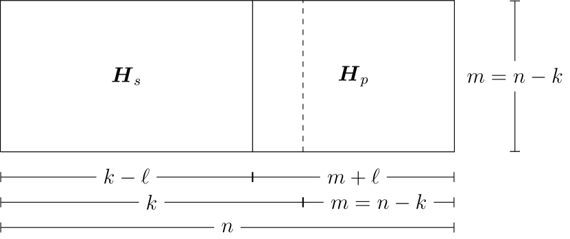
Figure 1: PPS divides the parity check matrix $\bm{H}$ into a syndrome former $\bm{H}_{s}$ and a non-square parity former $\bm{H}_{p}$.

Figure 2: LLPS encoding is achieved in two steps: (1) syndrome $\bm{s}=\bm{v}\bm{H}_{s}^{T}$ is calculated from the (shaped) systematic part $\bm{v}$. (2) the SDM calculates as parity part a shaped vector $\bm{p}$ with $\bm{p}\bm{H}_{p}^{T}=\bm{s}$. Without PPS, i.e., when $\bm{H}_{p}$ is square and $\bm{p}=\bm{s}(\bm{H}_{p}^{T})^{-1}$, the PAS [1] architecture is recovered.

II Preliminaries

Figure 3: PAS [1].

II-A Systematic Encoding

Consider an $(n,k)$ binary linear code $\mathcal{C}$ with block length $n$ and dimension $k$ and define $m=n-k$. We represent the code by an $m\times n$ parity check matrix $\bm{H}$, i.e.,

$$\mathcal{C}=\left\{\bm{c}\in\{0,1\}^{n}\colon\bm{c}\bm{H}^{T}=\bm{0}\right\}.$$ (3)

The code rate is $R_{\textnormal{fec}}=\frac{k}{n}$. Suppose that $\bm{H}$ decomposes as

$$\bm{H}=[\bm{H}_{s}|\bm{H}_{p}]$$ (4)

where $\bm{H}_{s}$ is $m\times k$ and $\bm{H}_{p}$ is $m\times m$ and has full rank. Then a length $k$ vector $\bm{v}$ can be systematically encoded into the codeword $[\bm{v}|\bm{p}]$ in two steps

1. Calculate the syndrome $\bm{s}=\bm{v}\bm{H}_{s}^{T}$.

2. Calculate the parity bits $\bm{p}=\bm{s}(\bm{H}_{p}^{T})^{-1}$.

Note that

$$[\bm{v}|\bm{p}]\bm{H}^{T}=\bm{v}\bm{H}_{s}^{T}+\bm{p}\bm{H}_{p}^{T}=\bm{s}+\bm{s}=\bm{0}$$ (5)

that is, by (3), $[\bm{v}|\bm{p}]$ is indeed a codeword.

II-B Linear Codes and Shaping

Consider a memoryless binary input channel $p_{Y|B}$. By [10], correct decoding is possible if the overhead $1-R_{\textnormal{fec}}$ fulfills

$$1-R_{\textnormal{fec}}>\operatorname{\mathbb{H}}(B|Y).$$ (6)

To relate code parameters to information measures, we consider (hypothetical) ideal codes with $1-R_{\textnormal{fec}}=\operatorname{\mathbb{H}}(B|Y)$. The number of check equations of an ideal linear code is then given by

$$m=n-k =n(1-R_{\textnormal{fec}})$$ (7)

$$=n\operatorname{\mathbb{H}}(B|Y).$$ (8)

II-C PAS

In PAS (see Fig. 3), length $k_{\textnormal{info}}\leq k$ information bits $\bm{u}$ are mapped by a DM to $k$ shaped bits $\bm{v}$ following the distribution $P_{V}$. The shaped bits $\bm{v}$ are then systematically encoded to the codeword $[\bm{v}|\bm{p}]$, as described in Sec. II-A. Consequently, the transmitted codeword has $k$ shaped bits $\bm{v}$ and $m$ unshaped parity bits $\bm{p}$ with the uniform distribution $P_{U}$. In higher-order modulation, the partially shaped codeword can be used for optimal signaling by using the shaped bits to address amplitudes and the unshaped bits to address signs [1].

The number of check equations $m$ of an ideal code is equal to the average uncertainty of PAS, i.e.,

$$m=n\left[R_{\textnormal{fec}}\operatorname{\mathbb{H}}(V|Y)+(1-R_{\textnormal{fec}})\operatorname{\mathbb{H}}(U|Y)\right].$$ (9)

By [13], the ideal DM has rate $\operatorname{\mathbb{H}}(V)$, so that

$$R=\frac{k_{\textnormal{info}}}{n}=\frac{\operatorname{\mathbb{H}}(V)k}{n}=\operatorname{\mathbb{H}}(V)R_{\textnormal{fec}}.$$ (10)

Combining (9) and (10), we get after some manipulations

$$R =R_{\textnormal{fec}}\operatorname{\mathbb{I}}(V;Y)+(1-R_{\textnormal{fec}})\operatorname{\mathbb{I}}(U;Y).$$ (11)

We see that the time sharing realized by PAS between shaped and unshaped channel inputs results in a time sharing achievable rate, which is in general suboptimal, by the concavity of mutual information in input distributions [14, Theorem 2.7.4].

III Probabilistic Parity Shaping

We now develop PPS, extending PAS by shaped parity bits.

III-A Modified Systematic Encoding

Consider Fig. 2 and Fig. 2. As in Sec. II-A, we consider an $(n,k)$ binary linear code with a $m\times n$ check matrix. We again partition the check matrix into $\bm{H}=[\bm{H}_{s}|\bm{H}_{p}]$, however, we modify the size of $\bm{H}_{s}$ and $\bm{H}_{p}$ to $m\times(k-\ell)$ and $m\times(m+\ell)$, respectively. The systematic encoding is as follows:

1. For length $k-\ell$ vector $\bm{v}$, calculate the syndrome $\bm{s}=\bm{v}\bm{H}_{s}^{T}$.

2. Calculate $m+\ell$ parity bits $\bm{p}$ by solving

   $$\bm{p}\colon\bm{p}\bm{H}_{p}^{T}=\bm{s}.$$ (12)

Since $\bm{H}_{p}$ is $m\times(m+\ell)$, the condition $\bm{p}\bm{H}_{p}^{T}=\bm{s}$ is fulfilled by many different solutions $\bm{p}$, consequently, we can choose the parity bits $\bm{p}$ subject to a shaping constraint. This is realized by an SDM, which we discuss in more detail next.

III-B SDM

For some cost function $f$, e.g., the Hamming weight

$$\textnormal{w}_{\textnormal{H}}(\bm{p})=\sum_{i}\bm{1}(p_{i}\neq 0)$$ (13)

where $\bm{1}(\text{true})=1$, $\bm{1}(\text{false})=0$, an SDM takes as input the length $m$ syndrome $\bm{s}$ and outputs a solution of

$$\bm{p}= \operatorname*{argmin}_{\bm{p}^{\prime}\in\{0,1\}^{m+\ell}}f(\bm{p}^{\prime})$$ (14)

subject to $$\bm{p}^{\prime}\bm{H}_{p}^{T}=\bm{s}.$$ (15)

We next detail an SDM realization that calculates all feasible vectors by (15) and then outputs the best according to (14). Let

$$\mathcal{C}_{p}=\left\{\bm{x}\in\{0,1\}^{\ell+m}\colon\bm{x}\bm{H}_{p}^{T}=\bm{0}\right\}$$ (16)

be the $\ell$-dimensional code defined by $\bm{H}_{p}$. The feasible vectors of (15) form the coset of $\mathcal{C}_{p}$ given by

$$\left\{\bm{x}+\tilde{\bm{p}}(\bm{s})\left|\bm{x}\in\mathcal{C}_{p}\right.\right\}$$ (17)

where $\tilde{\bm{p}}(\bm{s})$ is some particular solution of (15) used as representative of the coset. For $\bm{H}_{p}=[\bm{Q}|\bm{R}]$ with $\bm{R}$ square and full rank, a convenient representative is given by

$$\tilde{\bm{p}}(\bm{s})=[\bm{0}|\bm{s}(\bm{R}^{T})^{-1}].$$ (18)

The set of feasible vectors can now be calculated efficiently as follows.

1. Calculate offline $\mathcal{C}_{p}$ and store it in memory.

2. Calculate online $\tilde{\bm{p}}(\bm{s})=[\bm{0}|\bm{s}(\bm{R}^{T})^{-1}]$.

3. The set of solutions is $\{\mathcal{C}_{p}+\tilde{\bm{p}}(\bm{s})\}$.

III-C Rate Matching by LLPS

Suppose we use LLPS to encode into code words with distribution $P_{B}$. We realize the SDM by using as cost function the cross entropy

$$f(\bm{p})=\frac{1}{m+\ell}\sum_{i=1}^{m+\ell}\log_{2}\frac{1}{P_{B}(p_{i})}.$$ (19)

The ideal FEC code has $1-R_{\textnormal{fec}}=\operatorname{\mathbb{H}}(V|Y)$, the ideal DM has rate $k_{\textnormal{info}}/(k-\ell)=\operatorname{\mathbb{H}}(B)$, and the ideal SDM has rate $m/(m+\ell)=\operatorname{\mathbb{H}}(B)$, which translates into the following equations

$$m =n\operatorname{\mathbb{H}}(B|Y)$$ (20)

$$k_{\textnormal{info}} =\operatorname{\mathbb{H}}(B)(k-\ell)$$ (21)

$$m =\operatorname{\mathbb{H}}(B)(m+\ell).$$ (22)

We now have

$$R=\frac{k_{\textnormal{info}}}{n} =\operatorname{\mathbb{H}}(B)\frac{k-\ell}{n}$$ (23)

$$=\operatorname{\mathbb{H}}(B)\frac{k+m-m-\ell}{n}$$ (24)

$$=\operatorname{\mathbb{H}}(B)-\frac{\operatorname{\mathbb{H}}(B)(m+\ell)}{n}$$ (25)

$$=\operatorname{\mathbb{H}}(B)-\frac{m}{n}$$ (26)

$$=\operatorname{\mathbb{H}}(B)-\operatorname{\mathbb{H}}(B|Y)=\operatorname{\mathbb{I}}(B;Y).$$ (27)

We conclude that LLPS can operate at any rate between $0$ (for $\operatorname{\mathbb{H}}(V)=0$) and $R_{\textnormal{fec}}$ (for $\operatorname{\mathbb{H}}(V)=1$), and with ideal components, LLPS achieves the optimal achievable rate $\operatorname{\mathbb{I}}(B;Y)$.

III-D LLPS Decoding

The FEC decoder calculates its decision $[\hat{\bm{v}}|\hat{\bm{p}}]$ from the information it is provided by demapper. Since the transmitted $[\bm{v}|\bm{p}]$ is a code word, no change of the decoder is required. The decoder throws away the parity bits $\hat{\bm{p}}$ and outputs the decision $\hat{\bm{v}}$. For this, the only information required by the decoder is the value of $\ell$.

IV Dirty Paper Coding

Figure 4: Dirty paper coding scenario.

We now apply LLPS to a dirty paper coding scenario, where SDMs with small $\ell$, i.e., small computational cost, are sufficient to significantly improve the energy efficiency.

IV-A Channel Setup

We consider the scenario in Fig. 4. A binary sequence $b^{n}$ (not shown in Fig. 4) is mapped to a BPSK signal $x^{n}$, which is transmitted. The received signal $y^{n}$ is the sum of the transmitted signal $x^{n}$, an interfering BPSK signal $z^{n}$, and Gaussian noise $w^{n}$. The interfering signal $z^{n}$ is non-causally known to the transmitter, i.e., the binary sequence $b^{n}$ mapped to the transmitted signal $x^{n}$ is a function of the message $\bm{u}$ and the interfering signal $z^{n}$. At time instance $i$, we have

$$Y_{i}=\alpha x_{b_{i}}+\beta Z_{i}+W_{i}$$ (28)

where $W_{i}$, $i=1,\dotsc,n$ are independent and zero mean Gaussian with variance $\sigma^{2}$, where $z$ take values in $\{-1,1\}$, and where $x_{0}=-1$ and $x_{1}=+1$. The interference is uniformly distributed, i.e., $P_{Z}(-1)=P_{Z}(1)=\frac{1}{2}$. We define the signal-to-noise-ratio (SNR) by $10\log_{10}(\alpha^{2}/\sigma^{2})$ dB and we specify the strength of the interfering signal by $10\log_{10}(\beta^{2}/\alpha^{2})$ dB.

IV-B Reference Strategy: Interference as Noise

The transmitter ignores the presence of $z^{n}$ and the receiver treats the interfering signal as noise. The achievable rate for this reference strategy is

$$R =\operatorname{\mathbb{I}}(B;Y)$$

$$\qquad\text{$B$ and $Z$ independent, $B$ uniformly distributed}.$$ (29)

The demapper calculates the log-likelihood ratios

$$L(y)=\log\frac{p_{Y|B}(y|0)}{p_{Y|B}(y|1)}$$ (30)

where

$$p_{Y|B}(y|b)=\frac{1}{2}\left[p_{W}(y-\alpha x_{b}+\beta)+p_{W}(y-\alpha x_{b}-\beta)\right].$$ (31)

IV-C DPC

Using DPC (see, e.g., [15, Ch. 6]) we can achieve the rate

$$R_{\text{dpc}}=\operatorname{\mathbb{I}}(B;Y)-\operatorname{\mathbb{I}}(B;Z),\quad\text{$BZ\sim P_{Z}P_{B|Z}$}$$ (32)

by transmitting $B$ according to $P_{B|Z}$. The demapper calculates the LLR

$$p_{Y|B}(y|b)P_{B}(b)=\sum_{z\in\{-1,1\}}p_{Y|BZ}(y|bz)P_{BZ}(bz)$$ (33)

$$=\sum_{z\in\{-1,1\}}p_{Y|BZ}(y|bz)P_{B|Z}(b|z)\frac{1}{2}$$ (34)

$$=\sum_{z\in\{-1,1\}}p_{W}(y-\alpha x_{b}-\beta z)P_{B|Z}(b|z)\frac{1}{2}.$$ (35)

Remark 1.

We are considering the fixed bit-mapper $B\mapsto x_{B}$ with $x_{0}=-1$ and $x_{1}=+1$. By [15, Ch. 6], [16], in some cases, the DPC achievable rate (32) can be further improved by using a time variant bit-mapper that depends on $z_{i}$.

IV-D LLPS DPC Encoder

Figure 5: The constellation of $\alpha X+\beta Z$ and the distribution $P_{X+Z}$ resulting from $P_{B|Z}$. The optimized distribution prefers the outer constellation points, since they can be detected more reliably. The circles indicate $P_{X|Z}(\cdot|$-1$)P_{Z}($-1$)$ and the squares indicate $P_{X|Z}(\cdot|1)P_{Z}(1)$.

Figure 6: LLPS for dirty paper coding.

In Fig. 6, we display the LLPS for dirty paper coding. The DM for the systematic part $\bm{v}$ is instantiated by a SDM with matrix $\bm{H}_{\bm{v}}$, with an identity matrix to the right and entries at the left picked uniformly at random. Both SDMs get provided the corresponding part of the interfering signal. In Fig. 6, we display the distributions that we obtained from optimizing (32), see Sec. IV-F. The figure suggests that the SDMs should attempt to map 0 and 1 to the outermost signal points. Formally, define the label of the interfering signal by

$$a(z)=\begin{cases}0&z=-1\\ 1&z=1.\end{cases}$$ (36)

Then, the SDMs choose among the feasible vectors

$$\bm{v}^{*} =\operatorname*{argmin}_{\bm{v}}\textnormal{w}_{\textnormal{H}}(\bm{v}\oplus a_{1}^{k-\ell})$$ (37)

$$\bm{p}^{*} =\operatorname*{argmin}_{\bm{p}}\textnormal{w}_{\textnormal{H}}(\bm{p}\oplus a_{k-\ell+1}^{n}).$$ (38)

IV-E Ideal LLPS Rate

By (7), we know that the ideal FEC code has redundancy

$$m=n-k=\operatorname{\mathbb{H}}(B|Y)n.$$ (39)

Furthermore, we know that an ideal SDM has rate $\operatorname{\mathbb{H}}(B|Z)$. Thus, the rate of the DPC transmitter is

$$\frac{\operatorname{\mathbb{H}}(B|Z)(k-\ell)}{n} =\operatorname{\mathbb{H}}(B|Z)-\frac{\operatorname{\mathbb{H}}(B|Z)(n-k+\ell)}{n}$$ (40)

$$=\operatorname{\mathbb{H}}(B|Z)-\frac{n-k}{n}$$ (41)

$$=\operatorname{\mathbb{H}}(B|Z)-\operatorname{\mathbb{H}}(B|Y)$$ (42)

$$=\operatorname{\mathbb{I}}(B;Y)-\operatorname{\mathbb{I}}(B;Z)$$ (43)

which recovers the achievable rate (32).

IV-F Numerical Results

In Fig. 7, we show achievable rates for the considered DPC setup. The blue curve provides the reference for the interference-free scenario assuming Gaussian signaling. The orange and green curve represent the case with interference and $10\log_{10}(\beta^{2}/\alpha^{2})=$-5\text{\,}\mathrm{d}\mathrm{B}$$. We observe that the orange LLPS DPC curve gains $0.76\text{\,}\mathrm{d}\mathrm{B}$ over the reference scheme, which treats interference as noise (see Sec. IV-B). The employed non-uniform distribution $P_{B|Z}$ is obtained by maximizing $R_{\text{dpc}}$ in (32).

Figure 7: Information rates for different signaling schemes.

In Fig. 8, we show finite length simulation results that target a transmission rate of $R=$0.4697\text{\,}\mathrm{b}\mathrm{i}\mathrm{t}\mathrm{s}\mathrm{/}\mathrm{c}\mathrm{h}\mathrm{a}\mathrm{n}\mathrm{n}\mathrm{e}\mathrm{l}~{}\mathrm{u}\mathrm{s}\mathrm{e}$$ (bpcu). The interference-as-noise scheme uses a rate $1/2$ Wimax code [17] with blocklength $n=$1152\text{\,}\mathrm{b}\mathrm{i}\mathrm{t}\mathrm{s}$$, which is shortened by 66 bits to obtain the desired spectral efficiency. The LLPS DPC scheme uses a rate 1/2 Wimax code with blocklength $n=$1056\text{\,}\mathrm{b}\mathrm{i}\mathrm{t}\mathrm{s}$$. The distribution employed for calculating the decoder soft information in (35) is

$$P_{B|Z}=\begin{bmatrix}P_{B|Z}(0|$-1$)&P_{B|Z}(0|1)\\ P_{B|Z}(1|$-1$)&P_{B|Z}(1|1)\\ \end{bmatrix}=\begin{bmatrix}0.6037&0.3963\\ 0.3963&0.6037\\ \end{bmatrix}.$$

The outer SDM has rate $k_{\textnormal{info}}/(k-\ell)=496/(528-16)=$0.9688\text{\,}\mathrm{b}\mathrm{i}\mathrm{t}\mathrm{s}$$, and the inner SDM has rate $m/(m+\ell)=$0.9706\text{\,}\mathrm{b}\mathrm{i}\mathrm{t}\mathrm{s}$$. One hundred belief propagation iterations are performed. We observe gains of about $0.8\text{\,}\mathrm{d}\mathrm{B}$ in Fig. 8, recovering the asymptotic gain suggested by Fig. 7.

Figure 8: Finite length simulation results.

V Conclusions

We proposed a linear layered probabilistic shaping (LLPS) architecture that extends PAS by probabilistic parity shaping (PPS). LLPS integrates with any linear FEC and enables shaped parity bits, which are required, e.g., for optimized OOK. LLPS is a promising architecture for the probabilistic shaping problems considered in [7], [8], [4, Remark 3]. The enabling component of LLPS is a syndrome DM (SDM) defined on a $m\times(m+\ell)$ check matrix $\bm{H}_{p}$, which maps a syndrome to the vector in the corresponding coset that minimizes a cost function. LLPS was applied to a dirty paper coding problem, improving the energy efficiency by $0.8\text{\,}\mathrm{d}\mathrm{B}$. Future research should develop SDM algorithms that work efficiently also when neither $m$ nor $\ell$ are small.

References

- [1] G. Böcherer, F. Steiner, and P. Schulte, “Bandwidth efficient and rate-matched low-density parity-check coded modulation,” IEEE Trans. Commun., vol. 63, no. 12, pp. 4651–4665, Dec. 2015.
- [2] G. Böcherer, “Principles of coded modulation,” Habilitation thesis, Technical University of Munich, 2018. [Online]. Available: http://www.georg-boecherer.de/bocherer2018principles.pdf
- [3] R. A. Amjad, “Information rates and error exponents for probabilistic amplitude shaping,” in Proc. IEEE Inf. Theory Workshop (ITW), Guangzhou, China, Nov. 2018.
- [4] G. Böcherer, P. Schulte, and F. Steiner, “Probabilistic Shaping and Forward Error Correction for Fiber-Optic Communication Systems,” J. Lightw. Technol., vol. 37, no. 2, pp. 230–244, Jan. 2019.
- [5] P. Iannone, Y. Lefevre, W. Coomans, D. van Veen, and J. Cho, “Increasing cable bandwidth through probabilistic constellation shaping,” in Proc. SCTE-ISBE, 2018.
- [6] Y. C. Gültekin, W. J. van Houtum, S. Şerbetli, and F. M. Willems, “Constellation shaping for IEEE 802.11,” in Proc. IEEE Int. Symp. Personal, Indoor, Mobile Radio Commun. (PIMRC), 2017.
- [7] T. A. Eriksson, M. Chagnon, F. Buchali, K. Schuh, S. ten Brink, and L. Schmalen, “56 Gbaud probabilistically shaped PAM8 for data center interconnects,” in Proc. Eur. Conf. Optical Commun. (ECOC), 2017.
- [8] A. Git, B. Matuz, and F. Steiner, “Protograph-Based LDPC Code Design for Probabilistic Shaping with On-Off Keying,” in Proc. Ann. Conf. Inf. Sci. Syst. (CISS), Mar. 2019.
- [9] T. Wiegart, F. Steiner, and P. Yuan, “Shaped On-Off-Keying Transmission Using Polar Codes,” Mar. 2019, in preparation.
- [10] G. Böcherer, “Achievable rates for probabilistic shaping,” arXiv preprint, 2017. [Online]. Available: https://arxiv.org/abs/1707.01134v5
- [11] I. G. Gelfand and M. S. Pinkser, “Coding for channels with random parameters,” Prob. Contr. Inf. Theory, vol. 9, no. 1, pp. 19–31, 1980.
- [12] M. Costa, “Writing on dirty paper,” IEEE Trans. Inf. Theory, vol. 64, no. 2, pp. 439–441, May 1982.
- [13] P. Schulte and G. Böcherer, “Constant composition distribution matching,” IEEE Trans. Inf. Theory, vol. 62, no. 1, pp. 430–434, Jan. 2016.
- [14] T. M. Cover and J. A. Thomas, Elements of Information Theory, 2nd ed. John Wiley & Sons, Inc., 2006.
- [15] G. Kramer, “Topics in multi-user information theory,” Foundations and Trends in Comm. and Inf. Theory, vol. 4, no. 4–5, pp. 265–444, 2007.
- [16] D. Lentner, “Dirty paper coding for higher-order modulation and finite constellation interference,” Master’s thesis, Technical University of Munich, 2018.
- [17] “IEEE Standard for Local and Metropolitan Area Networks Part 16,” 2006.