Profile and Globe Tests of Mean Surfaces for Two-Sample Bivariate Functional Data

Abstract

Multivariate functional data has received considerable attention but testing for equality of mean surfaces and its profile has limited progress. The existing literature has tested equality of either mean curves of univariate functional samples directly, or mean surfaces of bivariate functional data samples but turn into functional curves comparison again. In this paper, we aim to develop both the profile and globe tests of mean surfaces for two-sample bivariate functional data. We present valid approaches of tests by employing the idea of pooled projection and by developing a novel profile functional principal component analysis tool. The proposed methodology enjoys the merit of readily interpretability and implementation. Under mild conditions, we derive the asymptotic behaviors of test statistics under null and alternative hypotheses. Simulations show that the proposed tests have a good control of the type I error by the size and can detect difference in mean surfaces and its profile effectively in terms of power in finite samples. Finally, we apply the testing procedures to two real data sets associated with the precipitation change affected jointly by time and locations in the Midwest of USA, and the trends in human mortality from European period life tables.

Keywords: Asymptotic Chi-square; Bivariate functional data; Globe test; Mean surface; Profile test.

1 INTRODUCTION

In multivariate functional stochastic process $X(u)$, there has increasing research interest in data type that is both functional and multidimentional. That is, $u=(s,t)$ has two arguments where $s\in\mathcal{S}\subset\mathbb{R}^{d_{1}}$ and $t\in\mathcal{T}\subset\mathbb{R}^{d_{2}}$ with $d_{1}$ and $d_{2}$ being positive integers. Here $s$ and $t$ inherently belong to distinct domains $\mathcal{S}$ and $\mathcal{T}$ in terms of scientific meaning or research design. For example, $X(s,t)$ may be the mortality rate of age $s$ during year $t$ in a given country. A typical example of such data comes from neuroimaging studies using functional magnetic resonance imaging (fMRI), in which the so-called voxels data, i.e. brain activity like blood flow changes are discrepantly recorded at a large number of locations at irregular time units (Lindquist, 2008; Aston and Kirch, 2012). Spatiotemporal study is no doubt another important application of this kind of data where $t$ is defined on a temporal domain and $s$ is defined on a spatial domain. Although functional data of afore structure are encountered in many applications, there is rare progress in inferential aspect for such data (Gromenko et al., 2017; Aston et al., 2017). In the present work, we plan to investigate the profile and globe tests of mean surfaces for two bivariate functional samples.

A practical motivation for this research comes from precipitation data in Midwest of the United States, where the daily data of precipitation from 1941 to 2000 are collected at 59 spatial locations scattered over 12 states in the Midwest of USA. For ease of reference, we provide a map of Midwest states with the locations of the climate monitoring stations in Figure 1. The Midwest is a breadbasket of the United States and its agriculture has continued to play a major role in the economy of the region (Pryor, 2013). The agriculture in the Midwest is vulnerably affected by the climate, of which precipitation is a vital component. To monitoring the future agricultural activities, it therefore has long been recognized as an important problem to reveal how the change of precipitation takes place for different locations, different regions, or different years in the same region.

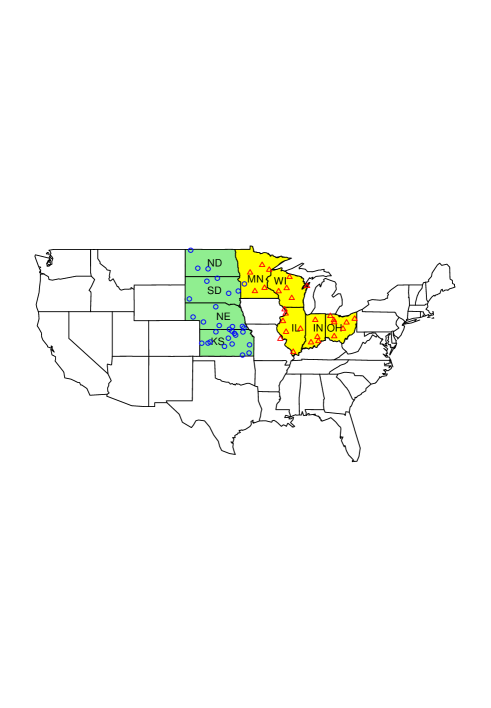
Figure 1: Light green region: 4 states from the Great Plains; Blue circle ${\color[rgb]{0,0,1}\circ}$ indicates location of a station; Yellow region: 5 states from the Great Lakes; Red triangle ${\color[rgb]{1,0,0}\triangle}$ indicates location of a station.

The study of the precipitation data has led to several interesting findings. For instance, Berkes et al. (2009) detected no changes during the period 1941-2000 for only individual station. However, it is difficult to implement if we sequently tested for every station when the number of stations were large. Gromenko et al. (2017) used cumulative sum paradigm to expose the fact that, the mean precipitation curves before and after 1966 were different over the whole region. Nevertheless their method was particularly designed to detect the temporal change but not applicable to detect the difference in spatio domain, not to mention the joint spatiotemporal effect on the precipitation. Looking into analysis of heatmaps of yearly sample mean surfaces where $X_{i}(s,t),i=1941,\cdots,1967$, corresponds to the precipitation of the $t$th day in the $i$th year at the $s$th station, intuitively we have observed that the yearly sample mean surface of precipitation in the Great Plains is different from that in the Great Lakes, refer to Figure 2. Also, we can recognize from Figure 2 that some profiles of mean surface are same but others are different. These motivate us to develop more powerful inferential procedures to detect if mean surfaces or its profiles have significant difference for either different regions or different individual stations.

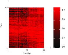
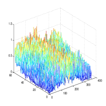
Figure 2: The heatmap of sample mean surface of precipitation during the time 1941-1967 in the Midwest, where the first 31 stations are located in the Great Plains and the latter 28 stations are located in the Great Lakes.

Tracking back testing procedures for the equality of mean functions in the functional data setting, existing works mainly focus on detecting the curve equality for univariate functional data. In the two-sample testing scenario, Benko et al. (2009) presented bootstrap procedures for testing the equality of mean curves through the eigenelements for two independent functional samples. Under the Gaussian assumption, Zhang et al. (2010) considered the two-sample test based on $L^{2}$-norm. Fremdt et al. (2014) derived mean functions comparison through a normal approximation method but only applicable to dense functional data samples. Pomann et al. (2016) still solved testing the curve equality problem though in bivariate (two-dimensional by their words) functional data setting and for distribution function testing. Regarding the $k$-sample testing or the one-way ANOVA for functional data, works include HANOVA (Fan and Lin, 1998), Cramér-von Mises type test (Cuevas et al., 2004; Estévez-Pérez and Vilar, 2013), $F$-type test (Ramsay and Silverman, 2005; Zhang, 2013; Zhang and Liang, 2014), B-spline test (Górecki and Smaga, 2015), and Mahalanobis distance (Ghiglietti et al., 2017), among others. In the case of within-curve dependence in each sample, Aston and Kirch (2012) detected the mean curve variation using $L^{2}$-norm criterion. Staicu et al. (2014) and its multiple group extension Staicu et al. (2015) worked on parametric testing relying on quite strong assumptions. Notice that, throughout our literature review, since our awareness concentrates on testing the equality of mean functions, we leave out other inferential topics such as testing the equality of coefficient operators or testing independency within a sample, and etc.

It has series of work in functional time series literature on testing the equality of mean functions, where weak dependence between or within two samples are accommodated in reality. Testing mean function difference in such functional time series study had still been on comparison of mean curve functions (Zhang et al., 2011; Horváth et al., 2013, 2014; Horváth and Rice, 2015a, b; Torgovitski, 2015, among others).

Aforementioned literature in both functional curve samples and functional time series have all inclined to testing the equality of mean curve functions, i.e. the inferential target is on univariate functional data. However, for comparison between samples of multivariate functional data, there have been few works by far. Only Gromenko et al. (2017) raised testing the equality of the mean surfaces of bivariate functional data, but eventually the equality of mean curves indexed at all locations were tested. Also to the best of our knowledge, the profile test of mean surfaces has not been considered for two bivariate functional data samples. Although the profile test of mean surfaces may belong to the curve test scope, it attributes to two different topics due to the different subjects. Above dire need in real-world data analysis and literature review motivates us to develop valid tests for equality of means surfaces and the corresponding profile test for bivariate functional data samples.

To address the problem in demand, firstly, we obtain the marginal eigen-function of the pooled sample by marginal functional principal component analysis (FPCA) and project the profiles of mean surfaces on marginal eigenfunctions. The profile testing statistic measures the distance of the profile of mean surfaces for two bivariate functional samples. Once the marginal eigenfunctions are obtained, the eigensurfaces of the pooled sample can be constructed by further FPCA. The distance between mean surfaces for two samples can be measured by the globe test statistic using the analogous projection ideas. Consequently, our proposed profile testing procedures can be implemented for every profile of the mean surface, which corresponds to simultaneously test whether mean precipitation curves have significant difference for every station. The globe test performs well in terms of both the size and the power in that it includes the information of two domains effectively.

The major contribution of this paper is threefold. Firstly, the presented methodology may be the first one to detect difference of mean surfaces and its profile for two-sample bivariate functional data. In contrast to the literature that we can search out by far, of which the focus has almost all been on testing the equality of mean curves as a matter of fact. When one argument is fixed, our profile test methodology can also simultaneously detect the mean difference in the other domain. Secondly, our testing procedures are interpretable and easily implemented. This will help fill out some theoretical gaps in functional inference and facilitate the real application and interpretation in statistical perspective. Finally, asymptotic distributions of the test statistics under null hypotheses has been derived. The consistency of test procedure has been proved. In addition, simulation studies show that the proposed tests have a good control of the type I error by the size and can detect difference in mean surfaces and its profile effectively in terms of power in finite samples.

The rest of the paper is organized as follows. In Section 2, we describe the model and data structure. The profile test procedure of mean surfaces for two bivariate functional data samples is presented in Section 3, while globe test procedure is proposed in Section 4. The finite sample performance for several representative scenarios is investigated in Section 5. In Section 6, we demonstrate two applications associated with the precipitation changes affected jointly by time and locations in the Midwest of USA, and the trends in human mortality from European period life tables. The paper concludes with a brief discussion in Section 7. Theory proofs are included in Supplementary.

2 MODEL AND DATA STRUCTURE

Let $L^{2}(\mathcal{S}\times\mathcal{T})$ be the separable Hilbert space. $\{X^{(m)}(s,t):(s,t)\in\mathcal{S}\times\mathcal{T}\}$ is a square integrable stochastic process on $L^{2}(\mathcal{S}\times\mathcal{T})$ with mean function $\mu_{m}(s,t)=E\{X^{(m)}(s,t)\}$ and covariance function

$$C^{(m)}\{(s,v),(u,t)\}=\text{E}\{X^{(m)c}(s,v)X^{(m)c}(u,t)\},$$

where $X^{(m)c}(s,t)=X^{(m)}(s,t)-\mu_{m}(s,t)$, for $m=1,2$, respectively. With this notation, we can decompose $X^{(m)}(s,t)$ into

$$\begin{array}[]{l}X^{(m)}(s,t)=\mu_{m}(s,t)+\varepsilon^{(m)}(s,t),m=1,2,\end{array}$$

where $\varepsilon^{(m)}(s,t)$ is the stochastic part of $X^{(m)}(s,t)$ with $\text{E}\{\varepsilon^{(m)}(s,t)\}=0$ and covariance function $C^{(m)}\{(s,v),(u,t)\}$.

Functional samples $\{X_{i}^{(m)}(s,t),m=1,2;i=1,\cdots,n_{m}\}$ may usually be modeled as independent realizations of the underlying stochastic process $X^{(m)}(s,t)$. In practice, $\{X_{i}^{(m)}(s,t),m=1,2;i=1,\cdots,n_{m}\}$ can not be observed, but rather, measurements are taken at discrete time points. In this paper, we assume $\{X_{i}^{(m)}(s,t),m=1,2;i=1,\cdots,n_{m}\}$ are recorded on a regular and dense grid of time points as follows,

$$\begin{array}[]{l}X_{i}^{(m)}(s_{il_{1}},t_{il_{2}})=\mu_{m}(s_{il_{1}},t_{il_{2}})+\varepsilon_{i}^{(m)}(s_{il_{1}},t_{il_{2}});\vspace{1mm}\\ m=1,2;\ i=1,\cdots,n_{m};\ l_{1}=1,\cdots,N;\ l_{2}=1,\cdots,M.\end{array}$$

In this paper, we are firstly interested in profile test of bivariate functional data samples, i.e. for every fixed $t^{*}\in\mathcal{T}$,

$$\begin{aligned} &H_{0}^{\mathcal{S}}:\mu_{1}(s,t^{*})=\mu_{2}(s,t^{*})\hskip 4.0pt\text{vs.}\hskip 4.0ptH_{1}^{\mathcal{S}}:\mu_{1}(s,t^{*})\neq\mu_{2}(s,t^{*}),\hskip 4.0pts\in\mathcal{S},\end{aligned}$$ (1)

or for every fixed $s^{*}\in\mathcal{S}$,

$$\begin{aligned} &H_{0}^{\mathcal{T}}:\mu_{1}(s^{*},t)=\mu_{2}(s^{*},t)\hskip 4.0pt\text{vs.}\hskip 4.0ptH_{1}^{\mathcal{T}}:\mu_{1}(s^{*},t)\neq\mu_{2}(s^{*},t),\hskip 4.0ptt\in\mathcal{T}.\end{aligned}$$ (2)

Then we go to the second target to present a globe test procedure for bivariate functional data samples with hypothesis below,

$$\begin{aligned} &H_{0}:\mu_{1}(s,t)=\mu_{2}(s,t)\hskip 4.0pt\text{vs.}\hskip 4.0ptH_{1}:\mu_{1}(s,t)\neq\mu_{2}(s,t),\hskip 4.0pts\in\mathcal{S},t\in\mathcal{T}.\end{aligned}$$ (3)

The equality in hypothesis (1) means that $\int_{\mathcal{S}}\{\mu_{1}(s,t^{*})-\mu_{2}(s,t^{*})\}^{2}ds=0$ for every fixed $t^{*}\in\mathcal{T}$, and the alternative means that $\int_{\mathcal{S}}\{\mu_{1}(s,t^{*})-\mu_{2}(s,t^{*})\}^{2}ds>0$. Analogously meaning can be interpreted for (2). However, null hypothesis of (3) implies $\int_{\mathcal{S}}\int_{\mathcal{T}}\{\mu_{1}(s,t)-\mu_{2}(s,t)\}^{2}dtds=0$ while the alternative means that $\int_{\mathcal{S}}\int_{\mathcal{T}}\{\mu_{1}(s,t)-\mu_{2}(s,t)\}^{2}dtds>0$. For statistical inference of bivariate functional data, marginal FPCA is a widely used tool, which often assumes that bivariate functional data can project onto finite-dimensional eigensurfaces (Li and Guan, 2014; Park and Staicu, 2015; Aston et al., 2017). It is our start point for the proposed profile and globe test procedures.

3 Profile test of bivariate functional data

Profile test of bivariate functional data is an important problem, as it allows to provide multiple insight from multiple angles, and also is of interest in many applications. For example, in analysis of precipitation, the testing problem (2) corresponds to test whether mean precipitation curves have significant difference before and after 1966 for every station, while the testing problem (1) means to test whether different stations have significant difference for every day. Berkes et al. (2009) considered detection the difference only on an individual station. However, it is difficult to implement when the number of stations is large if we sequentially test for every station by their method. So, we propose the profile test of mean functions which is easy to implement and can simultaneously detect difference of all stations. In this section, we address the test problem (1) only as (2) can be analogously implemented.

As a first step, the marginal covariance function is denoted to be $G_{\mathcal{S}}^{(m)}(s,u)=\int_{\mathcal{T}}C^{(m)}\{(s,t),(u,t)\}dt$, as the form of (5) in Chen et al. (2017), and may be estimated by

$$\begin{aligned} \widehat{G}_{\mathcal{S}}^{(m)}(s_{h},s_{l})={\displaystyle\frac{1}{n_{m}M}}\sum\limits_{i=1}^{n_{m}}\sum\limits_{k_{2}=1}^{M}&\widehat{X}_{i}^{(m)c}(s_{h},t_{ik_{2}})\\ &\times\widehat{X}_{i}^{(m)c}(s_{l},t_{ik_{2}}),\end{aligned}$$ (4)

where $\widehat{X}_{i}^{(m)c}(s,t)=X_{i}^{(m)}(s,t)-\overline{X}^{(m)}(s,t)$ with
$\overline{X}^{(m)}(s,t)={\displaystyle\frac{1}{n_{m}}}\sum\limits_{i=1}^{n_{m}}{X}_{i}^{(m)}(s,t)$.

Denote

$$\begin{array}[]{ll}\widehat{G}_{\mathcal{S}}(s,u)={\displaystyle\frac{n_{2}}{n_{1}+n_{2}}}\widehat{G}_{\mathcal{S}}^{(1)}(s,u)+{\displaystyle\frac{n_{1}}{n_{1}+n_{2}}}\widehat{G}_{\mathcal{S}}^{(2)}(s,u),\ s,u\in\mathcal{S}.\end{array}$$

It is easy to see $\widehat{G}_{\mathcal{S}}(s,u)\overset{p}{\longrightarrow}(1-\theta)G_{\mathcal{S}}^{(1)}(s,u)+\theta G_{\mathcal{S}}^{(2)}(s,u)\equiv G_{\mathcal{S}}(s,u)$, where $\theta$ is defined in Assumption 6 stated in next section and $G_{\mathcal{S}}(s,u)$ is the pooled covariance function. Consequently, it has orthogonal eigenfunctions $\{\psi_{j}\}_{j\geq 1}$ and non-negative eigenvalues $\{\nu_{j}\}_{j\geq 1}$ satisfying

$$\begin{array}[]{ll}&\displaystyle\int_{\mathcal{S}}G_{\mathcal{S}}(s,u)\psi_{j}(u)du=\nu_{j}\psi_{j}(s),\ s,u\in\mathcal{S},\ j=1,2,\ldots.\end{array}$$

Such eigencomponents can be numerically estimated by suitably discretized eigenequations,

$$\displaystyle\int_{\mathcal{S}}\widehat{G}_{\mathcal{S}}(s,u)\widehat{\psi}_{j}(u)du=\widehat{\nu}_{j}\widehat{\psi}_{j}(s),\ j=1,2,\ldots,$$ (5)

with orthogonal constraints on $\{\widehat{\psi}_{j}\}_{j\geq 1}$.

Once the estimators of marginal eigen-functions $\widehat{\psi}_{j}(s)$, $j=1,2,\ldots,$ are obtained, we project the observations onto the marginal eigenfunctions and obtain the profile estimators of mean functions as follows: for every fixed $t^{*}\in\mathcal{T}$,

$$\widehat{\mu}_{m}(s,t^{*})=\sum\limits_{j=1}^{J}\widehat{\eta}_{j}^{(m)}(t^{*})\widehat{\psi}_{j}(s),\ m=1,2,$$ (6)

with

$$\begin{aligned} &\widehat{\eta}_{j}^{(m)}(t^{*})={\displaystyle\frac{1}{n_{m}}}\sum\limits_{i=1}^{n_{m}}\widehat{\eta}_{ij}^{(m)}(t^{*}),\\ &\widehat{\eta}_{ij}^{(m)}(t^{*})={\displaystyle\frac{1}{N}}\sum\limits_{l_{1}=1}^{N}X_{i}^{(m)}(s_{il_{1}},t^{*})\widehat{\psi}_{j}(s_{il_{1}}).\end{aligned}$$

For practical implementation, one has to decide the magnitude of $J$. A practical strategy is $J=\min\{j:\frac{\widehat{\nu}_{1}+\widehat{\nu}_{2}+\cdots+\widehat{\nu}_{k}}{\widehat{\nu}_{l}+\widehat{\nu}_{2}+\cdots}>q\}$, where $\widehat{\nu}_{l}$, $l=1,2,\cdots$ are defined in (5). We find that $q=90\%$ threshold works well for our numerical examples.

Based on above discussion, we propose the following profile test statistic

$$\widehat{\text{TP}}(t^{*})={\displaystyle\frac{n_{1}n_{2}}{n_{1}+n_{2}}}\sum\limits_{j=1}^{J}{\displaystyle\frac{\left(\widehat{\eta}_{j}^{(1)}(t^{*})-\widehat{\eta}_{j}^{(2)}(t^{*})\right)^{2}}{\widehat{\lambda}_{j}(t^{*})}},$$

where $\widehat{\lambda}_{j}(t^{*})=\frac{n_{2}}{n_{1}+n_{2}}\widehat{\lambda}_{j}^{(1)}(t^{*})+\frac{n_{1}}{n_{1}+n_{2}}\widehat{\lambda}_{j}^{(2)}(t^{*})$ with
$\widehat{\lambda}_{j}^{(m)}(t^{*})=n_{m}^{-1}\sum_{i=1}^{n_{m}}\left\{\widehat{\eta}_{ij}^{(m)}(t^{*})-\widehat{\eta}_{j}^{(m)}(t^{*})\right\}^{2}$, $m=1,2$.

Remark 1

It is easy to see that $\frac{n_{1}n_{2}}{n_{1}+n_{2}}\int[\widehat{\mu}_{1}(s,t^{*})$
$-\widehat{\mu}_{2}(s,t^{*})]^{2}dt\overset{p}{\longrightarrow}U_{n_{1},n_{2}}=\frac{n_{1}n_{2}}{n_{1}+n_{2}}\sum_{l=1}^{K}(\widehat{\eta}_{l}(t^{*})-\widehat{\eta}_{2}(t^{*}))^{2}$. However, the variance of $U_{n_{1},n_{2}}$ may be unnecessarily inflated by the presence of, possibly many, very small estimates $\widehat{\mu}_{1}(s,t^{*})-\widehat{\mu}_{2}(s,t^{*})$. This drawback can be remedied by giving a divisor to $\widehat{\lambda}_{j}(t^{*})$.

We then establish asymptotic behaviors of the test statistic $\widehat{\text{TP}}(t^{*})$ under the null hypothesis $H_{0}^{\mathcal{S}}$ and the alternative one $H_{1}^{\mathcal{S}}$. To derive the asymptotic properties of profile test statistic, we make the following assumptions.

Assumption 1

$\nu_{1}>\nu_{2}>\cdots$ where $\{\nu_{j}\}_{j=1,2,\ldots}$ are the eigenvalues of covariance operates $G_{S}(s,u)$.

Assumption 2

For every fixed $t^{*}$, $\mu_{m}(s,t^{*}),m=1,2$ may be written as $\mu_{m}(s,t^{*})=\sum_{j=1}^{\infty}\eta_{j}^{(m)}(t^{*})\psi_{j}(s)$, where $\eta_{j}^{(m)}(t^{*})=\int_{0}^{1}\mu_{m}(s,t^{*})\psi_{j}(s)ds$.

Assumption 3

Assume $\sup_{(s,t)\in\mathcal{S}\times\mathcal{T}}\mu_{m}^{2}(s,t),m=1,2$ are bounded and $\text{E}(\sup|\varepsilon^{m}(s,t)|^{4}),m=1,2$ are bounded.

Assumption 4

The grid point $\{t_{il_{1}}:l_{1}=1,\ldots,N\}$ and $\{s_{il_{2}}:l_{2}=1,\ldots,M\}$ are equidistant. We assume $n_{1}/N^{2}=o(1)$, $n_{1}/M^{2}=o(1)$, $n_{2}/N^{2}=o(1)$ and $n_{2}/M^{2}=o(1)$.

Assumption 5

$\min\{n_{1},n_{2}\}\rightarrow\infty$, $n_{1}/(n_{1}+n_{2})\rightarrow\theta$ for a fixed constant $\theta\in(0,1)$.

Assumptions 1 and 3 are regular conditions. One needs these conditions to uniquely (up to signs) choose $\psi_{j}(s)$ and obtain the bound of $\widehat{\psi}_{j}(s)-\psi_{j}(s)$. Assumption 2 means that the profiles of mean surface are projected onto a space that is generated by a large set of basis functions. Assumption 4 requires that functional data are recorded on dense grid. Assumption 5 is of standard for two-sample asymptotic inference.

Theorem 1

Under Assumptions 1-5 and $H_{0}^{\mathcal{S}}$, we have $\widehat{\mathrm{TP}}(t^{*})\overset{d}{\longrightarrow}\chi_{J}^{2}$, where $\chi_{J}^{2}$ stands for a $\chi^{2}$ -distributed random variable with $J$ degrees of freedom. Under $H_{1}^{\mathcal{S}}$ and $0<\theta<1$, we have $\widehat{\mathrm{TP}}(t^{*})\overset{p}{\longrightarrow}\infty$.

From the expression of $\widehat{\mathrm{TP}}(t^{*})$ and remark 1, we can see that $\widehat{\mathrm{TP}}(t^{*})$ depends on sample sizes $n_{1},n_{2}$, and $\widehat{\eta}_{j}^{(1)}(t^{*})-\widehat{\eta}_{j}^{(2)}(t^{*}),j=1,\cdots,J$, which reflects the difference of profile mean functions $\mu_{1}(s,t^{*})$ and $\mu_{2}(s,t^{*})$. Intuitively, $\sqrt{\frac{n_{1}n_{2}}{n_{1}+n_{2}}}{(\widehat{\eta}_{j}^{(1)}(t^{*})-\widehat{\eta}_{j}^{(2)}(t^{*}))}\widehat{\lambda}_{j}^{-1/2}$ has a limiting standard normal distribution under $H_{0}^{\mathcal{S}}$. Theorem 1 shows that $\widehat{\text{TP}}(t^{*})$ asymptotically follows the chi-square distribution with $J$ degrees of freedom if $H_{0}^{\mathcal{S}}$ holds. Furthermore, $\widehat{\text{TP}}(t^{*})$ is consistent under $H_{1}^{\mathcal{S}}$. The proof of this theorem is provided in Supplementary.

4 Globe test of bivariate functional data

Compared with the profile test, the globe test of bivariate functional data attempts to detect the joint effects impacted by both domains. In this section, we develop a globe test method for bivariate functional data which aims to detect whether mean surfaces of precipitation have significant difference over a specific time window and/or a specific area, or whether two regions exist significant difference during different time windows.

Based on the estimated marginal eigenfunctions $\widehat{\psi}_{j}(s)$ in Section 3, we next estimate the marginal functional principal component scores $\widetilde{\xi}^{(m)}_{j,i}(t)$. The traditional integral estimates of $\widetilde{\xi}^{(m)}_{j,i}(t)$ based on the definition

$$\begin{aligned} &\widetilde{\xi}^{(m)}_{j,i}(t)=\int_{\mathcal{S}}X_{i}^{(m)c}(s,t)\widehat{\psi}_{j}(s)ds,\\ &i=1,\ldots,n_{m};\ j=1,2,\ldots.\end{aligned}$$

are

$$\begin{aligned} &\widehat{\xi}^{(m)}_{j,i}(t)=\sum_{l=2}^{N}X_{i}^{(m)c}(s_{l},t)\widehat{\psi}_{j}(s_{l})(s_{l}-s_{l-1}),\\ &i=1,\ldots,n_{m};\ j=1,2,\ldots.\end{aligned}$$ (7)

where $N$ is the number of measurements for $X_{i}^{(m)c}(s,t)$ in the direction $\mathcal{S}$.

Notice that each score function $\widehat{\xi}^{(m)}_{j,i}(t)$ is a centered new random curve. Denote the covariance function of $\xi_{j,i}^{(m)}(t)$ by $G_{\mathcal{T},j}^{(m)}(v,t)=E\{\xi_{j,i}^{(m)}(v)\xi_{j,i}^{(m)}(t)\}$. Then, the estimator of $G_{\mathcal{T},j}^{(m)}$ is denoted as,

$$\begin{aligned} &\widehat{G}^{(m)}_{\mathcal{T},j}(t_{h},t_{l})={\displaystyle\frac{1}{n_{m}}}\sum\limits_{i=1}^{n_{m}}\widehat{\xi}_{j,i}^{(m)}(t_{h})\widehat{\xi}_{j,i}^{(m)}(t_{l}),\\ &t_{h},t_{l}\in\mathcal{T};\ j=1,2,\ldots.\end{aligned}$$

Let

$$\begin{aligned} &\widehat{G}_{\mathcal{T},j}(v,t)={\frac{n_{2}}{n_{1}+n_{2}}}\widehat{G}^{(1)}_{\mathcal{T},j}(v,t)+{\displaystyle\frac{n_{1}}{n_{1}+n_{2}}}\widehat{G}^{(2)}_{\mathcal{T},j}(v,t),\\ &v,t\in\mathcal{T};\ j=1,2,\ldots.\end{aligned}$$

It is easy to see $\widehat{G}_{\mathcal{T},j}(v,t)\overset{p}{\longrightarrow}(1-\theta)G^{(1)}_{\mathcal{T},j}(v,t)+\theta G^{(2)}_{\mathcal{T},j}(v,t)$
$\equiv G_{\mathcal{T},j}(v,t)$ where $G_{\mathcal{T},j}(v,t)$ is the covariance function and has orthogonal eigenfunctions $\{\phi_{jk}\}_{k\geq 1}$ and non-negative eigenvalues $\{\nu_{jk}\}_{k\geq 1}$ satisfying

$$\begin{aligned} &\int_{\mathcal{T}}G_{\mathcal{T},j}(v,t)\phi_{jk}(v)dv=\nu_{jk}\phi_{jk}(t),\\ &v,t\in\mathcal{T};\ k,j=1,2,\ldots.\end{aligned}$$

Then estimators of eigenvalues and eigenfunctions $\{(\nu_{jk},\phi_{jk}(t)):j,k\geq 1\}$ are obtained by the following equations,

$$\displaystyle\int_{\mathcal{T}}\widehat{G}_{\mathcal{T},j}(v,t)\widehat{\phi}_{jk}(v)dv=\widehat{\nu}_{jk}\widehat{\phi}_{jk}(t),\ k,j=1,2,\ldots,$$ (8)

with orthogonal constraints on $\{\widehat{\phi}_{jk}\}_{k\geq 1}$.

Denote $\varphi_{jk}(s,t)\equiv\phi_{jk}(t)\psi_{j}(s)$ and its consistent estimator by $\widehat{\varphi}_{jk}(s,t)=\widehat{\phi}_{jk}(t)\widehat{\psi}_{j}(s)$. We propose estimators of the mean surfaces which are projection of observations onto a hyperspace spanned from the pooled eigensurfaces $\{\widehat{\varphi}_{jk}(s,t):j,k\geq 1\}$, written as

$$\widehat{\mu}_{m}(s,t)=\sum\limits_{j=1}^{J}\sum\limits_{k=1}^{K_{j}}\widehat{\eta}_{jk}^{(m)}\widehat{\varphi}_{jk}(s,t),\ m=1,2,$$ (9)

with

$$\begin{aligned} &\widehat{\eta}_{jk}^{(m)}={\displaystyle\frac{1}{n_{m}}}\sum\limits_{i=1}^{n_{m}}\widehat{\eta}_{ijk}^{(m)},\\ &\widehat{\eta}_{ijk}^{(m)}={\displaystyle\frac{1}{MN}}\sum\limits_{l_{2}=1}^{M}\sum\limits_{l_{1}=1}^{N}X_{i}^{(m)}(s_{il_{1}},t_{il_{2}})\widehat{\varphi}_{jk}(s_{il_{1}},t_{il_{2}}),\end{aligned}$$

where selection of $J$ is the same to in Section 3 and $K_{j}$ can be decided by analogous procedure. In details, we select $K_{j}=\min\{k:\frac{\widehat{\nu}_{j1}+\widehat{\nu}_{j2}+\cdots+\widehat{\nu}_{jk}}{\widehat{\nu}_{j1}+\widehat{\nu}_{j2}+\cdots}>0.9\}$, where $\widehat{\nu}_{jl}$, $l=1,2,\cdots$ are defined in (8).

It is natural to take into consideration the term $\widetilde{\text{TC}}\equiv\int_{\mathcal{S}}\int_{\mathcal{T}}\{\mu_{1}(s,t)-\mu_{2}(s,t)\}^{2}dtds$ to measure the distance between two estimated mean surfaces. It is readily seen that $\widetilde{\text{TC}}\overset{p}{\longrightarrow}\sum\limits_{j=1}^{J}\sum\limits_{k=1}^{K_{j}}\left(\widehat{\eta}_{jk}^{(1)}-\widehat{\eta}_{jk}^{(2)}\right)^{2}$. Therefore, $H_{0}$ will be rejected if $\widetilde{\text{TC}}$ is large. Similarly, the variance of $\widetilde{\text{TC}}$ may be unnecessarily inflated by the presence of, possibly many, very small estimates $\widehat{\eta}_{jk}^{(1)}-\widehat{\eta}_{jk}^{(2)}$. This drawback can also be remedied by giving a divisor to their variance.

Based on the above steps, we propose the following test statistic

$$\begin{array}[]{ll}\widehat{\text{TM}}={\displaystyle\frac{n_{1}n_{2}}{n_{1}+n_{2}}}\sum\limits_{j=1}^{J}\sum\limits_{k=1}^{K_{j}}{\displaystyle\frac{\left(\widehat{\eta}_{jk}^{(1)}-\widehat{\eta}_{jk}^{(2)}\right)^{2}}{\widehat{\lambda}_{jk}}},\end{array}$$

where $\widehat{\lambda}_{jk}=n_{2}(n_{1}+n_{2})^{-1}\widehat{\lambda}_{jk}^{(1)}+n_{1}(n_{1}+n_{2})^{-1}\widehat{\lambda}_{jk}^{(2)}$ with $\widehat{\lambda}_{jk}^{(m)}=(n_{m}-1)^{-1}\sum_{i=1}^{n_{m}}\left(\widehat{\eta}_{ijk}^{(m)}-\widehat{\eta}_{jk}^{(m)}\right)^{2}$, $m=1,2$.

From (9), we can see that $X_{i}^{(1)}(\cdot,\cdot)$ and $X_{i}^{(2)}(\cdot,\cdot)$ are directly projected on the common basis surface and obtain $\widehat{\eta}_{ijk}^{(1)}$ and $\widehat{\eta}_{ijk}^{(2)}$. $\widehat{\eta}_{jk}^{(1)}$ and $\widehat{\eta}_{jk}^{(2)}$, which are the average of such projection, and hence can be viewed as the scores of projection that two mean surfaces $\mu_{1}(s,t)$ and $\mu_{2}(s,t)$ project on the same basis function space, respectively. The representation of $\widehat{\text{TM}}$ measures the total such deviation between two samples. Therefore, the proposed method has a nice explanation and easy to implement.

Next we establish asymptotic behavior of the test statistic $\widehat{\text{TM}}$ under hypotheses (3). Additionally, we need the following assumptions.

Assumption 6

$\nu_{j1}>\nu_{j2}>\cdots$ where $\{\nu_{jk}\}_{k=1,2,\ldots;j=1,2,\ldots}$ are the eigenvalues of the covariance function $G_{T}(v,t)$.

Assumption 7

Assume $\mu_{m}(s,t),m=1,2$ may be written as $\mu_{m}(s,t)=\sum_{j=1}^{\infty}\sum_{k=1}^{\infty}\eta_{jk}^{(m)}\varphi_{jk}(s,t)$, where $\eta_{jk}^{(m)}=\int_{0}^{1}\int_{0}^{1}\mu_{m}(s,t)\varphi_{jk}(s,t)dsdt$.

Assumption 6 along with Assumption 3 in Section 3 ensures the bound of $\widehat{\phi}_{jk}(t)-\widehat{\phi}_{jk}(t)$. The interpretation of Assumption 7 is similar to Assumption 2 in Section 3.

Theorem 2

Under Assumptions 1-7 and $H_{0}$, we have

$$\begin{array}[]{llll}\widehat{\mathrm{TM}}\overset{d}{\longrightarrow}\chi_{\sum\limits_{j=1}^{J}K_{j}}^{2},\end{array}$$

where $\chi_{\sum_{j=1}^{J}K_{j}}^{2}$ stands for a $\chi^{2}$-distributed random variable with $\sum_{j=1}^{J}K_{j}$ degrees of freedom. Under $H_{1}$ and $0<\theta<1$, we have $\widehat{\mathrm{TM}}\overset{p}{\longrightarrow}\infty$.

Intuitively $\sqrt{\frac{n_{1}n_{2}}{n_{1}+n_{2}}}\left(\widehat{\eta}_{jk}^{(1)}-\widehat{\eta}_{jk}^{(2)}\right)\widehat{\lambda}_{jk}^{-1/2}$ has a limiting standard normal distribution under $H_{0}$. Theorem 2 shows that $\widehat{\text{TM}}$ asymptotically follows the chi-square distribution with $\sum\limits_{j=1}^{J}K_{j}$ degrees of freedom under $H_{0}$. The consistency of $\widehat{\text{TM}}$ is also illustrated under $H_{1}$, which together provides clear theoretical justification of the empirical properties of the proposed test. The proof of this theorem is provided in Supplementary.

5 Simulation studies

We conduct extensive simulation studies and report two representative examples here. Examples 1 and 2 evaluate two proposed testing procedures in terms of empirical size and power when covariance functions of two samples are identical or distinct, separately. The data grid for argument $s$ consists of 100 equispaced points on $[0,1]$, and the grids for argument $s$ consists of 50 equispaced points on $[0,1]$. Each pair of data-generated processes was replicated 1000 times.

Example 1

Identical covariance functions.

In this example, we consider the following model

$$\begin{aligned} &X_{i}^{(1)}(s,t)=\varepsilon_{i}^{(1)}(s,t),\ i=1,\ldots,n_{1},\\ &X_{i}^{(2)}(s,t)=\delta(s+t)+\varepsilon_{i}^{(2)}(s,t),\ i=1,\ldots,n_{2},\end{aligned}$$ (10)

where $\varepsilon_{i}^{(1)}(s,t)$ and $\varepsilon_{i}^{(2)}(s,t)$ are independently generated from

$$\varepsilon(s,t)=\sum\limits_{j=1}^{2}\xi_{j}(t)\psi_{j}(s),\ s\in[0,1],t\in[0,1],$$

with $\psi_{1}(s)=s^{2}$ and $\psi_{2}(s)=s^{3}$, $s\in[0,1]$. $\xi_{j}(t)$ is generated from

$$\begin{array}[]{llll}\xi_{j}(t)=\sum\limits_{k=1}^{2}\chi_{jk}\phi_{jk}(t),\ j=1,2,\end{array}$$

with $\phi_{11}(t)=\phi_{21}(t)=-\surd 2\cos(2\pi t)$, $\phi_{12}(t)=\phi_{22}(t)=\surd 2\sin(2\pi t)$, $t\in[0,1]$; $\chi_{11}\sim N(0,3)$, $\chi_{12}\sim N(0,1.5)$, $\chi_{21}\sim N(0,2)$, and $\chi_{22}\sim N(0,1)$.

Example 2

Distinct covariance functions.

To compare with Example 1, we consider the following model

$$\begin{aligned} &X_{i}^{(1)}(s,t)=\varepsilon_{i}^{(1)}(s,t),\ i=1,\ldots,n_{1},\\ &X_{i}^{(2)}(s,t)=\delta(s+t)+\varepsilon_{i}^{(2)}(s,t),\ i=1,\ldots,n_{2},\end{aligned}$$ (11)

where $\varepsilon_{i}^{(1)}(s,t)$ is generated from

$$\begin{array}[]{llll}\varepsilon^{(1)}(s,t)=\sum_{j=1}^{2}\xi_{j}(t)\psi_{j}(s),\ s\in[0,1],t\in[0,1],\end{array}$$

and $\varepsilon_{i}^{(2)}(s,t)$ from

$$\begin{array}[]{llll}\varepsilon^{(2)}(s,t)=\xi_{1}(t)\psi_{1}(s),\ s\in[0,1],t\in[0,1],\end{array}$$

with $\psi_{1}(s)=s^{2}$ and $\psi_{2}(s)=s^{3}$, $s\in[0,1]$. $\xi_{j}(t)$ is generated from

$$\begin{array}[]{llll}\xi_{j}(t)=\sum\limits_{k=1}^{2}\chi_{jk}\phi_{jk}(t),\ j=1,2,\end{array}$$

with $\phi_{11}(t)=\surd 2\cos(2\pi t)$, $\phi_{21}(t)=\surd 2\sin(2\pi t)$, $\phi_{12}(t)=2\cos(4\pi t)$, $\phi_{22}(t)=2\sin(4\pi t)$, $t\in[0,1]$; $\chi_{11}\sim N(0,3)$, $\chi_{12}\sim N(0,1.5)$, $\chi_{21}\sim N(0,2)$, and $\chi_{22}\sim N(0,1)$.

Example 1 can be seen as two-sample tests where covariance functions are identical, while covariance functions of Example 2 are distinct. The sample size pair is taken to be $(n_{1},n_{2})=(25,75)$, $(50,150)$, $(100,300)$, $(50,50)$, $(100,100)$, and $(200,200)$, respectively. The empirical sizes of profile test are computed for different $s$ and $t$. To save space, we here only present the results of different $s$ for $(n_{1},n_{2})=(100,100)$ in Figure 3. Next, we can also compute the empirical sizes of the globe test. The results are reported in Table 1. The empirical power can be evaluated when $\delta\neq 0$. The empirical power at $\delta=0.4,0.6,0.8$ of profile tests are displayed in Figure 4 while the results of globe tests at $\delta=0.2,0.4,0.6,0.8,1.0,1.2$ are scatter plotted in Figure 5.

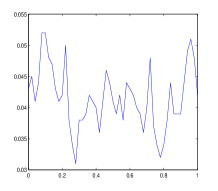
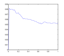
Figure 3: The results of empirical size when covariance functions of two samples are identical (left column) and distinct (right column).

Table 1: Empirical sizes of two proposed test procedures in Examples 1 and 2.

$(n_{1},n_{2})$	(50,50)	(100,100)	(200,200)	(25,75)	(50,150)	(100,300)
Example 1	0.079	0.060	0.050	0.111	0.085	0.061
Example 2	0.074	0.064	0.048	0.080	0.062	0.048

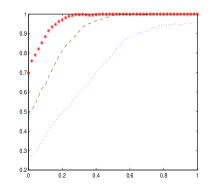
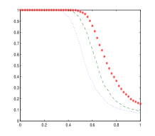
Figure 4: The results of empirical power when covariance functions of two samples are identical (left column) and distinct (right column).

Several observations can be concluded from Figures 3 and 4. Firstly, the profile tests have a good control of the type I error. The empirical sizes of identical covariance scenarios are better than that of distinct covariance cases. Secondly, the empirical power of the test becomes larger when $\delta$ increases from 0.4 to 0.8, which is expected. Lastly, the empirical power for the same covariance case is slightly larger than that of the different covariance function cases.

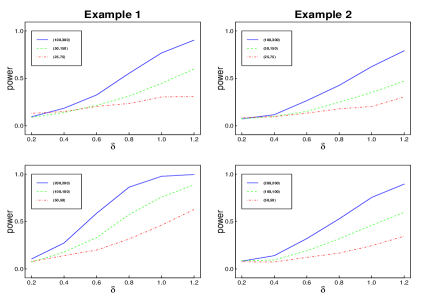
Figure 5: The results of empirical power when covariance functions of two samples are identical (left column) and distinct (right column). Top: The results of empirical power of $(n_{1},n_{2})=(25,75)$ (red), $(50,150)$ (green) and $(100,300)$ (blue). Bottom: The results of empirical power of $(n_{1},n_{2})=(50,50)$ (red), $(100,100)$ (green) and $(200,200)$ (blue).

We may observe from Table 1 and Figure 5 that the globe test approach can keep steady empirical size even at pairs of small sample sizes $(n_{1},n_{2})=(25,75)$ or $(50,50)$. The empirical power of two test methods increases as the sample size increases. When $\delta$ increases from 0.2 to 1.2, the empirical power of the test becomes more and more large, which is evidence of the consistency of the testing procedures. Also the empirical power of equal sample size scenario is slightly better than that of unequal sample size one.

6 Real data examples

To illustrate profile and globe tests methods, we analyse the historical precipitation data in the Midwest of USA and the period lifetables in Europe for human mortality trend analysis.

6.1 Precipitation data

The first example is used to analyze the changes of precipitation during 1941-2000 or in different regions in the Midwest of USA. Berkes et al. (2009) detected no changes during the period 1941-2000 for only one station while Gromenko et al. (2017) detected the change of precipitation during 1941-2000 over the whole region.

The precipitation data is available from the global historical climatological network database. The comprehensive U.S. Climate Normals dataset includes various derived products including daily air temperature normals, precipitation normals and hourly normals. The dataset that we analyzed in this paper can be downloaded directly from GHCN (Global Historical Climatology Network)-Daily, an integrated public database of NOAA (https://www.ncdc.noaa.gov/oa/climate/ghcn-daily/) by an R interface. Our interest is daily precipitation records from Midwestern states including Illinois, Indiana, Iowa, Kansas, Michigan, Minnesota, Missouri, Nebraska, North Dakota, Ohio, South Dakota, and Wisconsin. In Figure 1, totally 59 locations of the climate monitoring stations are indicated with blue circles ${\color[rgb]{0,0,1}\circ}$ in 4 states from the Great Plains (light green region), and with red triangles ${\color[rgb]{1,0,0}\triangle}$ in 5 states from the Great Lakes (yellow region). Notice that there is no climate monitoring stations in Iowa, Michigan, and Missouri. We target to detect whether the changes of average precipitation took place for different time phases or regions.

Let $Y_{i}(s,t)$ be the precipitation of the $t$th day in the ith year of the $s$th station. Before we apply the proposed method, we need to do registration with the data. To remove the effects due to the heavy tail distribution, we apply the transformation

$$Z_{i}(s,t)=\log_{10}\{Y_{i}(s,t)+1\},$$

where $\{Y_{i}(s,t)\}$ are original records. After the transformation, we pre-smooth data by using the cubic splines function. It is noted that the data of every climate monitoring stations from 1941 to 2000 can be constituted into a time series with length 21900(365 day by 60 year). Then, the data of the 59 climate monitoring stations can be seen as a sample with sample size being 21900 and variables being 59. According to the empirical Pearson correlation of 59 variables, the 59 climate monitoring stations is stringed into a function by the stringing method in Chen et al. (2011). Consequently the spatiotemporal data $\{Y_{i}(s,t)\}$ are converted into the bivariate functional data $\{X_{i}(s,t)\}$. Notice that the difference between the spatiotemporal data $Y_{i}(s,t)$ and the bivariate functional data $X_{i}(s,t)$ is that the argument $s$ in the former expression has no order but it is ranked in the latter.

Gromenko et al. (2017) studied the data $Y_{i}(s,t)$ and detected out the change of the average precipitation at about 1967. In this subsection, we firstly apply the profile test to check if the profile of mean surfaces are equal during the periods 1941-1967 and 1968-2000. It corresponds to test whether the average precipitation of every station has changes during these periods. The $p$-values of the profile tests are computed and results are displayed in Figure 6. As can be seen from Figure 6, most of the $p$-values are less than 0.05 or significant except 11 stations. For ease of reference, we list the latitude and longitude in Table 2 for 11 stations. This displays that the average precipitation of most locations had changed during the periods 1941-1967 and 1968-2000.

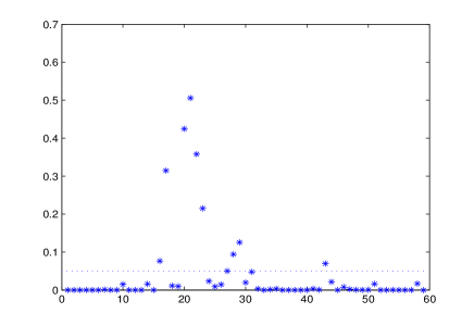
Figure 6: The $p$-value of the profile tests for every station.

Table 2: The latitude and longitude of stations where the $p$-value of profile test are more than 0.1.

Code	latitude	longitude
USC00148235	38.4661	-101.7758
USC00250050	42.5522	-99.8556
USC00252145	41.4086	-102.9661
USC00255090	40.8508	-101.5428
USC00325479	46.8128	-100.9097
USC00394007	43.4378	-103.4739
USC00398307	45.4283	-101.0764
USC00394007	43.4378	-103.4739
USC00392797	45.7644	-99.6353
USC00321871	48.9075	-103.2944
USC00327530	46.8886	-102.3192

Next, we implement the following globe test

$$\begin{aligned} &H_{0}^{\text{Midwest}}:\mu_{1}(s,t)=\mu_{2}(s,t)\\ &\text{vs.}\hskip 4.0ptH_{1}^{\text{Midwest}}:\mu_{1}(s,t)\neq\mu_{2}(s,t),s\in\mathbb{R}^{59},t\in\mathbb{R}^{365}.\end{aligned}$$

From the globe test procedure presented in Section 4 together with the asymptotic distribution of the test statistic $\widehat{\text{TM}}$, we calculate the corresponding $p$-value to be 0.001. This result is consistent with the conclusion of Gromenko, Kokoszka and Reimherr. That is, the patterns of mean surfaces are different over the whole Midwest region between before 1967 and after 1967. Intuitively, according to the results of the profile test, the precipitation had changed in most of locations which lead to the variations of whole region.

The heatmaps in Figure 2 leak the information that sample mean values of annual precipitation in the Great Lakes (GL) based on 28 stations are more than that in the Great Plains (GP). This motivates us to further explore how the mean functions of bivariate functional data $\{X_{i}(s,t)\}$ was affected by temporal and spatial effects from both domains. It is natural to test the equality of two mean surfaces of the precipitation for the 31 stations located in the GP and the 28 stations located in the GL during the periods 1941-1967 and 1968-2000, respectively by

$$H_{0}^{1967-}:\mu^{\text{GP}}=\mu^{\text{GL}}\hskip 4.0pt\text{vs.}\hskip 4.0ptH_{1}^{1967-}:\mu^{\text{GP}}\neq\mu^{\text{GL}},$$

and

$$H_{0}^{1967+}:\mu^{\text{GP}}=\mu^{\text{GL}}\hskip 4.0pt\text{vs.}\hskip 4.0ptH_{1}^{1967+}:\mu^{\text{GP}}\neq\mu^{\text{GL}}.$$

All the $p$-values by globe test procedures for above two hypotheses are tiny approaching to zero indicating rejecting the null hypotheses but in favor of the alternative one. It is consistent with the intuition that the mean patterns of precipitation at Great Plains and at Great Lakes are different.

Furthermore, for the 28 stations located in the GL, we test the mean surfaces of precipitation before and after 1967, denoted by

$$H_{0}^{\text{GL}}:\mu^{1967-}=\mu^{1967+}\hskip 4.0pt\text{vs.}\hskip 4.0ptH_{1}^{\text{GL}}:\mu^{1967-}\neq\mu^{1967+}.$$

The $p$-value is 0.0163. The null hypothesis would be rejected at 0.05 significance level. Testing equality of the mean surfaces of precipitation before and after 1967 is also implemented for the 31 stations located in the GP, denoted by

$$H_{0}^{\text{GP}}:\mu^{1967-}=\mu^{1967+}\hskip 4.0pt\text{vs.}\hskip 4.0ptH_{1}^{\text{GP}}:\mu^{1967-}\neq\mu^{1967+}.$$

The $p$-values by globe testing method are 0.5677. The null hypothesis would not be rejected at 0.05 significance level. That is, averagely speaking, the precipitation in the Great Lakes changed before 1967 and after 1967, whereas the mean pattern of precipitation in the Great Plains had no change before 1967 and after 1967. Therefore, our analysis provides evidence that change in the mean function of precipitation was mainly due to the Great Lakes but the Great Plains may be affected little. By looking up the map, we find that all the stations in Table 2 are located in the Great Plains. It further verify the reliability of the proposed methods. All testing results are presented in Table 3.

Table 3: Results of the tests based on statistics $\widehat{\text{TM}}$.

statistic	the observed value of a statistic	$p$-value
$H_{0}^{\text{Midwest}}:\mu^{1967-}(s,t)=\mu^{1967+}(s,t)$
$\begin{array}[]{c}\widehat{\text{TM}}\end{array}$	$\begin{array}[]{c}123.6\end{array}$	$\begin{array}[]{c}\textbf{0.001}\end{array}$
$H_{0}^{\text{GP}}:\mu^{1967-}(s,t)=\mu^{1967+}(s,t)$
$\begin{array}[]{c}\widehat{\text{TM}}\end{array}$	$\begin{array}[]{c}59.7175\end{array}$	$\begin{array}[]{c}0.5677\end{array}$
$H_{0}^{\text{GL}}:\mu^{1967-}(s,t)=\mu^{1967+}(s,t)$
$\begin{array}[]{c}\widehat{\text{TM}}\end{array}$	$\begin{array}[]{c}108.20\end{array}$	$\begin{array}[]{c}\textbf{0.0163}\end{array}$
$H_{0}^{1967-}:\mu^{\text{GP}}(s,t)=\mu^{\text{GL}}(s,t)$
$\begin{array}[]{c}\widehat{\text{TM}}\end{array}$	$\begin{array}[]{c}973.11\end{array}$	$\begin{array}[]{c}\textbf{0.0000}\end{array}$
$H_{0}^{1967+}:\mu^{\text{GP}}(s,t)=\mu^{\text{GL}}(s,t)$
$\begin{array}[]{c}\widehat{\text{TM}}\end{array}$	$\begin{array}[]{c}1116.4\end{array}$	$\begin{array}[]{c}\textbf{0.0000}\end{array}$

6.2 European human mortality rate data

In the second example, we will analyse the trends in human mortality based on the records in the period life tables during the calendar years 1960-2006 for Europe countries. A period life table represents the mortality conditions at a specific moment in time. It is approachable from the Human Mortality Database via the website linkage www.mortality.org (Wilmoth et al., 2007). The analysis of trends in human mortality is important to recover the demographic impacts. Results of such research will benefit the prediction and forecasting of future cohort mortality (Vaupel et al., 1998; Oeppen and Vaupel, 2002). We focus on comparison of different countries or genders, specifically on the older ages over 50 years old.

There are 32 countries included in the European period life tables. It contains five Eastern European countries, Belarus, Bulgaria, Russia, Ukraine and Lithuania, and the remaining 27 Western European countries. Following the notation introduced in Section 3, $X_{i}^{(1)}(s,t),i=1,\ldots,5,$ denotes the mortality rate of the five Eastern European countries for subjects at age $s$ and calendar year $t$, where $50\leq s\leq 90$, focusing on the death rates of older individuals, and on a recent block of 47 years, $1960\leq t\leq 2006$. Similarly, $X_{i}^{(2)}(s,t),i=1,\ldots,27,$ denotes the mortality rate for other countries. The sample mean function $\widehat{\mu}_{1}(s,t)=\sum_{i=1}^{5}X_{i}^{(1)}(s,t)$ and $\widehat{\mu}_{2}(s,t)=\sum_{i=1}^{27}X_{i}^{(2)}(s,t)$ for two clusters of countries are visualized in Figure 7. The heatmaps and sample mean surfaces show obvious opposite trend of mortality rates particularly for very aged people in Eastern and Western European countries as the calendar year passed 1980 or so. We apply the profile and globe test procedures to test if the two underlying mean surfaces and its profile are different.

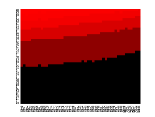
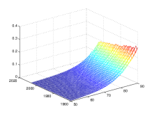
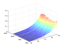
Figure 7: Top: Sample means of the mortality rate for the 5 Eastern European countries. Bottom: Sample means of the mortality rate for the 27 Western European countries.

According to profile test method introduced in Section 3, we implement the tests (1) and (2). The $p$-values for fixed $s^{*}$ or $t^{*}$ are calculated, respectively. The results are presented in Figure 8. For every fixed age $s^{*}$, we find that all of $p$-values are approaching to zero. This indicates that the mean mortality rates of the Eastern and Western European is different for every age $s^{*}=50,\cdots,90$. For every fixed year $t^{*}$, almost all $p$-values are less than 0.05 except for years $t^{*}=1978$ and $1986$. Sequentially, we implement the globe test for the mean mortality rates of the Eastern and Western European. The numbers of included components is $J=2,K_{1}=2,K_{2}=2$ are chosen by the fraction of variance explained (FVE) criterion with the threshold 0.90. Based on the asymptotic distribution of the test statistic $\widehat{\text{TM}}$, the $p$-value is calculated to be 0. It coincides with the intuition on images in Figure 7 and is evidence that the mean surfaces of the mortality rates are different between the Eastern and Western European countries. Also, it is consistent with the conclusion of the profile test because almost of $H_{0}^{\mathcal{S}}$ and $H_{0}^{\mathcal{T}}$ are rejected for fixed $s^{*}$ and $t^{*}$.

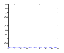
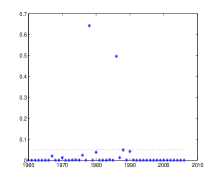
Figure 8: The $p$-value of the profile tests for every age (left) and year(right).

Next we examine the equality of mean surfaces and its profile between female and male clusters in West Europe. The heatmaps and sample mean surfaces for male and female clusters are displayed in Figure 9. Intuitively it does not show obvious difference. However, all the $p$-values of profile tests are zero for fixed $s^{*}$ and $t^{*}$. Furthermore, we also implement globe test and obtain the $p$-value that is 0. Therefore, the mean surface and its profile are different in Western Europe for aged people in different gender type.

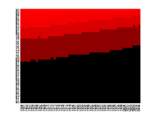
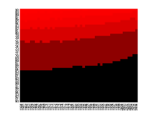
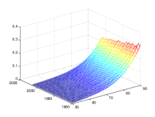
Figure 9: Top: Sample means of the mortality rate of male. Bottom: Sample means of the mortality rate of female.

7 Discussion

Bivariate functional data have been definitely presented in Park and Staicu (2015), Chen et al. (2017) and
Aston et al. (2017). However, inferential in testing procedures of such data type has not been adequately dealt with in the literature. This paper develops profile and globe tests to detect if mean surfaces and their profile are different for two bivariate functional samples.

In this paper, for simplicity, we assume $X^{(m)}(s,t)$ are recorded on a regular and dense grid of pair time point. It is noted that the mean function and its profile estimation in (6) and (9) can always be obtained in the sparse and irregular setting by additional smoothing steps. Our proposed profile and globe tests can also be implemented if marginal eigenfunctions and mixed eigenfunctions can be effectively estimated. Hence, the proposed testing methodology will have wider application and much more flexible framework.

Additionally, for bivariate functional data $X^{(m)}(s,t)$, product functional principal component analysis (PFPCA) due to Chen et al. (2017) and double functional principal component analysis (DFPCA) due to Chen and Müller (2012) have been developed. Using the methodology similar to Section 3 and 4, profile and globe tests based on PFPCA and DFPCA can also be developed.

Higher dimensional functional data also occur in practice. For example, in a recent environment and conservation project, the raw water sample has been collected weekly from different branch streams of Dongjiang at Pearl River Delta, China. Quite a few water quality indices were measured for each sample. The measurements database form naturally a trivariate functional data. To save cost and to monitor water quality more effectively, we are interested in detecting whether water quality has significantly changed across time, locations and water quality indices. The corresponding null hypothesis is thus then

$$H_{0}:\mu_{1}(b,s,t)=\mu_{2}(b,s,t)\hskip 4.0pt\text{vs.}\hskip 4.0ptH_{1}:\hskip 4.0pt\mu_{1}(b,s,t)\neq\mu_{2}(b,s,t),$$

where $\mu_{i}(b,s,t)$ is the mean function for the $i$th sample $\{X_{i}(b,s,t)\}_{i=1}^{n_{i}},i=1,2$ with sample size $n_{i}$ collected on time $t$ at location $s$ with water quality index $b$ measured. Although as mentioned earlier that the methods developed can be similarly extended to more than two samples, technical derivations become tedious. We are currently working on methods for trivariate or higher order multivariate functional data.

SUPPLEMENTARY MATERIAL

Proof of Theorem

This file is to present the detail of the proof procedure of the corresponding theorems in the article. (file type: pdf)

References

- (1)
- Aston and Kirch (2012) Aston, J., and Kirch, C. (2012), “Detecting and estimating changes in dependent functional data,” Journal of Multivariate Analysis, 109, 204–220.
- Aston et al. (2017) Aston, J., Pigoli, D., and Tavakoli, S. (2017), “Tests for separability in nonparametric covariance operators of random surfaces,” Annals of Statistics, p. To appear.
- Benko et al. (2009) Benko, M., Härdle, W., and Kneip, A. (2009), “Common functional principal components,” Annals of Statistics, 37(1), 1–34.
- Berkes et al. (2009) Berkes, I., Gabrys, R., Horváth, L., and Kokoszka, P. (2009), “Detecting changes in the mean of functional observations,” Journal of the Royal Statistical Society, Ser. B, 71(5), 927–946.
- Chen et al. (2011) Chen, K., Chen, K., Müller, H.-G., and Wang, J.-L. (2011), “Stringing high-dimensional data for functional analysis,” Journal of the American Statistical Association, 106(493), 275–284.
- Chen et al. (2017) Chen, K., Delicado, P., and Müller, H.-G. (2017), “Modeling function-valued stochastic processes, with applications to fertility dynamics,” Journal of the Royal Statistical Society, Ser. B, 79(1), 177–196.
- Chen and Müller (2012) Chen, K., and Müller, H.-G. (2012), “Modeling repeated functional observations,” Journal of the American Statistical Association, 107(500), 1599–1609.
- Cuevas et al. (2004) Cuevas, A., Febrero, M., and Fraiman, R. (2004), “An anova test for functional data,” Computational Statistics and Data Analysis, 47, 111–122.
- Estévez-Pérez and Vilar (2013) Estévez-Pérez, G., and Vilar, J. (2013), “Functional ANOVA starting from discrete data: an application to air quality data,” Environmental and Ecological Statistics, 20, 495–517.
- Fan and Lin (1998) Fan, J., and Lin, S.-K. (1998), “Test of significance when data are curves,” Journal of the American Statistical Association, 98(443), 1007–1021.
- Fremdt et al. (2014) Fremdt, S., Horváth, L., Kokoszka, P., and Steinebach, J. (2014), “Functional data analysis with increasing number of projections,” Journal of Multivariate Analysis, 124, 313–332.
- Ghiglietti et al. (2017) Ghiglietti, A., Leva, F., and Paganoni, A. (2017), “Statistical inference for stochastic processes: two-sample hypothesis tests,” Journal of Statistical Planning and Inference, 180, 49–68.
- Górecki and Smaga (2015) Górecki, T., and Smaga, Ł. (2015), “A comparison of tests for the one-way ANOVA problem for functional data,” Computational Statistics, 30(4), 987–1010.
- Gromenko et al. (2017) Gromenko, O., Kokoszka, P., and Reimherr, M. (2017), “Detection of change in the spatiotemporal mean function,” Journal of the Royal Statistical Society, Ser. B, 79(1), 29–50.
- Horváth et al. (2013) Horváth, L., Kokoszka, P., and Reeder, R. (2013), “Estimation of the mean of functional time series and a two-sample problem,” Journal of the Royal Statistical Society, Ser. B, 75(1), 103–122.
- Horváth et al. (2014) Horváth, L., Kokoszka, P., and Rice, G. (2014), “Testing stationarity of functional time series,” Journal of Econometrics, 75(1), 103–122.
- Horváth and Rice (2015a) Horváth, L., and Rice, G. (2015a), “An introduction to functional data analysis and a principal component approach for testing the equality of mean curves,” Revista Matemática Complutense, 28, 505–548.
- Horváth and Rice (2015b) Horváth, L., and Rice, G. (2015b), “Testing equality of means when the observations are from functional time series,” Journal of Time Series Analysis, 36, 84–108.
- Li and Guan (2014) Li, Y., and Guan, Y. (2014), “Functional principal component analysis of spatiotemporal point processes with applications in disease surveillance,” Journal of the American Statistical Association, 109(507), 1205–1215.
- Lindquist (2008) Lindquist, M. (2008), “The statistical analysis of fMRI data,” Statistical Science, 23(4), 439–464.
- Oeppen and Vaupel (2002) Oeppen, J., and Vaupel, J. (2002), “Broken limits to life expectancy,” Science, 296, 1029–1031.
- Park and Staicu (2015) Park, S., and Staicu, A. (2015), “Longitudinal functional data analysis,” Stat, 4, 212–226.
- Pomann et al. (2016) Pomann, G., Staicu, A., and Ghosh, S. (2016), “A two-sample distribution-free test for functional data with application to a diffusion tensor imaging study of multiple sclerosis,” Journal of the Royal Statistical Society, Ser. C, 65(3), 395–414.
- Pryor (2013) Pryor, S. (2013), Climate Change in the Midwest: Impacts, Risks, Vulnerability, and Adaptation Indiana University Press.
- Ramsay and Silverman (2005) Ramsay, J., and Silverman, B. (2005), Functional Data Analysis New York: Springer.
- Staicu et al. (2015) Staicu, A.-M., Lahiri, S., and Carroll, R. (2015), “Significance tests for functional data with complex dependence structure,” Journal of Statistical Planning and Inference, 156, 1–13.
- Staicu et al. (2014) Staicu, A.-M., Li, Y., Crainiceanu, C., and Ruppert, D. (2014), “Likelihood ratio tests for dependent data with applications to longitudinal and functional data analysis,” Scandinavian Journal of Statistics, 41, 932–949.
- Torgovitski (2015) Torgovitski, L. (2015), “Detecting changes in Hilbert space data based on “repeated” and change-aligned principal components,” Preprint ArXiv: 1509.07409, .
- Vaupel et al. (1998) Vaupel, J., Carey, J., Christensen, K., Johnson, T., Yashin, A., Holm, N., Iachine, I., Kannisto, V., Khazaeli, A., Liedo, P., Longo, V., Zeng, Y., Manton, K., and Curtsinger, J. (1998), “Biodemographic trajectories of longevity,” Science, 280(5365), 855–860.
- Wilmoth et al. (2007) Wilmoth, J., Andreev, K., Jdanov, D., and Glei, D. (2007), “Methods protocol for the Human Mortality Database, (version 5),” Technical Report, .
- Zhang (2013) Zhang, J.-T. (2013), Analysis of Variance for Functional Data CRC press.
- Zhang and Liang (2014) Zhang, J.-T., and Liang, X. (2014), “One-way ANOVA for functional data via globalizing the pointwise F-test,” Scandinavian Journal of Statistics, 41(1), 51–71.
- Zhang et al. (2010) Zhang, J.-T., Liang, X., and Xiao, S. (2010), “On the two-sample Behrens-Fisher problem for functional data,” Journal of Statistical Theory and Practice, 4, 571–587.
- Zhang et al. (2011) Zhang, X., Shao, X., Hayhoe, K., and Wuebbles, D. (2011), “Testing the structural stability of temporally dependent functional observations and application to climate projections,” Electronic Journal of Statistics, 5, 1765–1796.