Ab initio calculations of 5H resonant states
Abstract
By solving the 5-body Faddeev-Yakubovsky equations in configuration space with realistic nuclear Hamiltonians we have studied the resonant states of 5H isotope. Two different methods, allowing to bypass the exponentially diverging boundary conditions, have been employed providing consistent results. The existence of 5H broad Jπ=1/2+,3/2+,5/2+ states as S-matrix poles has been confirmed and compared with the, also calculated, resonant states in 4H isotope. We have established that the positions of these resonances only mildly depend on the nuclear interaction model.
keywords:
4H and 5H , Faddeev-Yakubovsky equations , Few-Nucleon problem , ab initio calculations1 Introduction
Neutron-proton unbalanced nuclei are a unique laboratory to study the isospin dependence of the nuclear interaction as well as the nuclear properties far beyond the stability line. Hydrogen isotopes play a special role, as they provide the extreme neutron to proton ratios and thus are actively studied both theoretically as well as experimentally.
If there seems to be a general agreement between the experimentalist on the existence of several resonances in 5H isotope [1, 2, 3, 4], the parameters of these resonances vary significantly from one experiment to another. These discrepancies might be attributed to the different reaction mechanism leading to the formation of broad resonant states and to the difficulty in identifying their quantum numbers. Indeed, in any physical observable, the contributions of broad resonances strongly interfere among themselves as well as with a non-resonant background, producing in the resonance region a response, which strongly depends on the particular reaction mechanism. Unless the reaction mechanism is well understood and one is able to isolate – analytically or numerically – both contributions, the resonance parameters are not defined in a unique way. In this case only qualitative analysis of the experimentally extracted broad resonance parameters makes sense.
According to the results of Korsheninnikov et al. [2] the lowest resonant state of 5H would be narrower than the ones of 4H isotope, a fact that could be naively attributed to the additional attraction provided by the subsystem present in 5H relative to one present in 4H. Or, alternatively, to the pairing effect over a core of 3H. By extending this effect to one could in this way obtain a natural explanation for the extremely narrow parameters of the 7H resonance published in [5].
The findings of ref. [2] were confirmed by Golovkov et al. [3], attributing even smaller widths to the 5H resonant states. They are however in conflict with a recent work [4] where the resonance width was found to be much larger and comparable with the one of the 4H ground state, although this difference could be partially attributed to the different reaction mechanism used in their production.
Several theoretical works on this system were performed in the past. They could be classified in two major groups: t-n-n models in which 3H nuclei is considered as a point like particle (hereafter denoted by ) and microscopic 3-body cluster models, based on 3H+n+n structure. In t-n-n models, the Pauli principle between the valence neutrons and those contained in the 3H core is mimicked by a repulsive term in the effective t-n interaction. In contrast, microscopic models start from a bare Nucleon-Nucleon (NN) interaction and employ properly antisymmetrized 5-nucleon wave functions, however some severe constrains on the dynamics of the 3H core are applied.
These studies were pioneered by Shul’gina et al. [6], where 5H is described by a t-n-n model, solved by means of hyperspherical Harmonics techniques. The t-n potential was taken from the same authors [7] and the one from Gogny et al. [8]. Within the same approach, a theoretical study of broad states in few-body systems beyond the neutron drip line was published in [9]. No precise positions were given but studies of the sensitivity of the 5H spectrum to reaction mechanism predict that the ”ground state” peak may be observed at 2-3 MeV as lowest position, though could be shifted to much higher energies in certain situations.
In [10] a similar 3-body model but with a refined t-n interaction was considered with taken from [11]. The positions of 5H resonant states were computed by means of the Complex Scaled (CS) hyperspherical adiabatic expansion method. However, this model failed to obtain realistic 5H resonant states when using only two-body interactions; adjustment of an additional ad-hoc t-n-n 3-body force was required to reproduce the positions of the Jπ=1/2+,3/2+,5/2+ states. The energy distributions of the fragments after their decay were computed as well.
A t-n-n model was also used, in the framework of hypernuclear physics [12], to compute 5H resonant states. The problem was solved by combining CS with the Gaussian expansion method [12]. The interaction was Argonne V8’ [13] and one was adapted from [14]. It was found again, that this 3-body model failed to reproduce ground state resonance parameters unless some ad-hoc 3-body force was included and properly adjusted.
The first microscopic model for 5H using the Generator Coordinate Method (GCM) was used in [15]. The key ingredient of the calculation, the NN potential, was based on semi-realistic Minnesota (MN) [16] and Mertelmeier and Hofmann [17] models. Resonance parameters were identified using the analytic continuation in a coupling constant (ACCC) method [18]. In a later work [19] this last study was improved, replacing the GCM technique by a 3-body microscopic approach based on Hypersherical Harmonics method.
A microscopic three cluster model of 5H, using the equivalent Resonating Group Method (RGM) approach and the MN potential, was also presented in [20].
Finally, a microscopic cluster model of 5H was presented in [21], based on 3-cluster J-matrix method (MJM) and Hyperspherical Harmonics basis. Resonance positions were directly computed by imposing the appropriate boundary conditions. Different components of the MN and modified Hasegawa-Nagata potentials [22] were used to built the NN interaction.
It seems firmly established that the t-n-n models of 5H systematically require a properly adjusted t-n-n 3-body force in order to produce 5H resonant states with reasonable widths. Thus, their predictions critically depends on 3-body force parameters on which there is little control. On the contrary, all microscopic models agree on the existence of a relatively broad Jπ=1/2+ resonant state in 5H, which is located 1.5 MeV above the 3H threshold and has a width in the range of 1-3 MeV. The presence of even broader Jπ=3/2+ and Jπ=5/2+ states has been also indicated. These methods however rely on 3-cluster wave functions and employ simplistic phenomenological NN interactions. As we will see in what follows, their predictions display also some dispersion even when using the same interaction.
We believe it could be of interest to determine unambiguously the S-matrix pole position of these resonant states by undertaking the ab initio solution of this problem with the only input of a realistic NN interaction. Indeed, our recently developed techniques, allowing to solve the 5-body Faddeev-Yakubovsky equations in configuration space, and for the first time applied to calculate n-4He elastic phase shifts [23, 24], provide us the opportunity to investigate the properties of 5H nucleus from an ab initio theoretical perspective. By solving the 5-nucleon problem in the complex energy plane we present here the first ab initio study of 5H, involving no approximations on the dynamics.
A new experiment has been recently performed at RIKEN [25], combining benefits of radioactive ion beam facilities and multineutron detection arrays, aiming to resolve the puzzle of observable 4n and 7H states. Understanding the evolution of H-isotope resonances, originated from S-matrix poles in the vicinity of the real energy axis, when increasing the number of neutrons was one of the main motivations of our work. Therefore our theoretical attempt is timely and hopefully will also be relevant for a better understanding and interpretation of the experimental data.
2 Formalism
Faddeev-Yakubovsky (FY) equations were formulated in [26], as an extension of the seminal work of Faddeev [27] for a 3-particle system (A=3) to an arbitrary number of particles (A=N). Starting from the middle 80’s, they have been successfully solved both in momentum and configuration space for A=4 in all possible bound and scattering channels [28, 29, 30]. The first results for A=5 problem, recently obtained by one of the authors [23, 24], introduced the formalism in some detail. In this letter we will just highlight the main ideas.


In the FY approach, the intrinsic (center of mass) 5-body wave function depending on four vector variables , is decomposed into 180 components corresponding to the five different topologies in the cluster partition of the system, which are represented in Fig. 1. Subscript denotes their topological type and the superscript the sequence of particle indexes.
These components are naturally expressed in their proper set of Jacobi coordinates , , . These are represented in the lower panel of Fig.1 and have the generic form
where denotes the center of mass positions of the two clusters (eventually single particles) connected by each coordinate and their reduced mass. An arbitrary mass is introduced to keep the physical units.
For a system of identical particles with mass one chooses . One can also choose a preferential particle ordering , say , and the permutation symmetry allows to reduce the number of independent components to only five , one for each topological type. The remaining components, as well as the total wave function, can be reconstructed from this subset with the help of coordinate basis transformation operators :
| (1) | |||
| (2) |
Using the completeness relation one may split any operator into a product of simpler transformation operators , similar to the ones used in the 3-body case [24], which affect only two vector coordinates at once and let unchanged the functional dependence of the remaining two:
| (3) |
As discussed in [24] a set of eleven such operators is sufficient to express any complicated transformation appearing in the solution of a 5-body problem.
The FY components correspond to the different asymptotic channels and satisfy a coupled system of second order partial differential equations. In view of solving these equations, a partial wave expansion on each vector variables is performed
where is a generalized ”quadripolar harmonic” function accounting for the angular momentum, spin and isospin couplings
() holds for the spin (isospin) couplings and labels the set of quantum numbers involved in the intermediate couplings. The above expressions represents the main coupling scheme used in this work for the K, H, S and F topologies. For T topology a slightly modified coupling scheme was used, obtained by permuting particle 3 and 5 indexes for spin and isospin couplings. These coupling schemes allow to (anti)symmetrize the total wave function in a trivial way.
After projecting the angular part, one is left with a set of coupled four-dimensional integro-differential equations for the reduced radial amplitudes in the form
| (4) |
where
and is the two-body potential (multiplied by ).
In the right hand side of eq. (4), an integration over the angular variables and , allowing to connect the Jacobi coordinate sets and , is performed. This essential operation is realized in the matrix form by breaking the integration in three successive steps, as briefly explained in eqs.(1-3). The radial dependence of these amplitudes is sought by expanding them in the Lagrange-Laguerre basis functions using the Lagrange-mesh method [31]. In our numerical calculation, the partial wave basis was limited to . The number of Lagrange-mesh points to expand the radial FY components was for the -coordinate and for and . The errors introduced by these truncations are smaller than the uncertainties related with the methods used to calculate the positions of the resonant states.
To access the complex energy eigenvalues of a resonant state, we have used the method of Analytic Continuation in the Coupling Constant (ACCC) in the same form as in our previous works [32, 33, 34] and we have developed a variant of the Smooth Exterior Complex Scaling method (SECS) that will be detailed in what follows.
ACCC does not allow a direct determination of resonance parameters. These are obtained by artificially binding the system with an ”external field” driven by a strength parameter and computing its binding energy as a function of this parameter: . In our case, we added to 5H Hamiltonian a fictitious 5-body hyperradial potential on the form:
| (5) |
Equation (4) should be accordingly modified by adding to its left hand side the term .
Several values of were calculated up to 3H+n+n threshold, corresponding to the critical strength , above which the 5H S-matrix pole moves into the resonance region. These values are used to determine a Padé-like functional dependence in the domain of real arguments
which will be analytically continued in the complex plane until , where the external potential is fully removed (). At this point, the position of the 5H resonance relative to 3H threshold may be easily determined. As it was explained in [34, 35, 36], in the context of 3n and 4n systems, the use of an artificial 5-body force to bind 5H is motivated by the compelling need to avoid spurious branching points, related to the appearance of artificially bound 5H subsystems.
In our previous studies we have extensively employed the CS method to calculate resonance parameters as well as several scattering observables [37]. Nevertheless, the conventional CS fails in describing broad resonant states for they require a large rotation angle to be exposed. Furthermore, some short range potentials, like e.g. chiral NN interactions, include sharp vertex form factors and start to diverge already when very moderate values of are used.
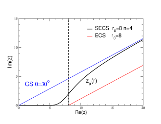
To tackle this problem, the so called Exterior Complex Scaling method (ECS) was proposed [38], which applies the CS transform only in the region free from interaction, say with sufficiently large. However, in its standard form, ECS has a formal inconsistency when applied to the problem solved via partial wave decomposition, due to the interplay between different Jacobi coordinate sets. To circumvent this problem we propose an analytic mapping – hereafter denoted SECS – whose effect is extremely small in the interaction region and, hence, it is applied to the kinetic energy term only. If this mapping is performed by means of a sharp enough function centered outside of interaction region, SECS gives very accuracy results. In practice it can be realized by the means of a smooth step-like function :
| (6) |
which is represented in Fig. 2 (right panel) together with its ancestors.
We illustrate this method with a two-body P-wave resonance generated by the potential:
| (7) |
with =2589.696 MeV, =1128.393 MeV, =3.11 fm-1, =1.55 fm-1 and =41.471 MeV fm2. In this example we took , but the method applies well for larger angles.
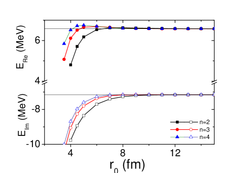
We have plotted in Figure 2 (left panel) the complex energy values of the resonance as a function of , the range parameter of SECS, calculated with the mapping (6) and n=4 displayed in right panel. As one may see, results are indistinguishable from the exact S-matrix pole +i=6.578-i 7.1578 MeV for 8 fm. With 12 fm, one reproduces four significant digits using and , while the differences using differs only by 1 keV. Despite the fact that our approach neglects the transformation of the potential energy, it produces stable and very accurate results.
When solving FY equations in sector, it is of interest to apply SECS to hyperradius only, for it allows a consistent treatment of the kinetic energy operators in different Jacobi coordinate sets. We have successfully realized this option in 3-body calculations, but it is worth noticing that the transformation of four radial Jacobi coordinates turned to be even a better choice. The last procedure slightly breaks the consistency of the kinetic energy in the different FY components. Nevertheless when working with radial Jacobi coordinates we are able to evaluate the transformed kinetic energy terms more accurately if the transformation is natural to these coordinates, which turns out to be a critical ingredient in the calculations requiring sharp regulators.
3 Results
In this work three different NN interactions have been considered: two realistic ones and a third one semi-realistic. Among the first, the I-N3LO chiral EFT potential of Entem and Machleidt [39] which was very successful in describing the n-3H elastic cross section near the resonance peak even without corresponding three nucleon forces [40], and the INOY non-local potential from [41] which provides an accurate description of A=2,3,4 binding energies. The semi-realistic S-wave MT13 potential [42] was also considered which, despite its bare simplicity, describes well the gross properties of low energy few-nucleon systems.
| I-N3LO | 1.15(5) | 3.97(7) | 0.90(3) | 3.80(8) | 0.78(15) | 7.7(7) | 0.2(2) | 4.6(1) |
| INOY | 1.31(4) | 4.16(4) | 0.96(7) | 4.03(8) | 0.80(15) | 8.3(1) | 0.2(2) | 5.0(1) |
| MT13 | 1.08(3) | 4.06(5) | 1.08(3) | 4.06(5) | 1.08(3) | 4.06(5) | 0.88(9) | 4.4(1) |
| RGM [20] | 1.52 | 4.11 | 1.23 | 5.80 | 1.19 | 6.17 | 1.32 | 4.72 |
| tn [10] | 1.22 | 3.34 | 1.15 | 3.49 | 0.77 | 6.72 | 1.15 | 6.38 |
| Exp. [44] | 3.19 | 5.42 | 3.50 | 6.73 | 5.27 | 8.92 | 6.02 | 12.99 |
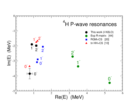
We have first computed the Jπ=2-,0-,1- P-wave resonances of its closest isotope 4H, which dominate the low energy n-3H elastic cross section in the peak region and which are intimately related with the resonant states in 5H. The method used here is a direct calculation of the 4N resonant state by solving the FY equations with the techniques developed in [33, 43] supplied with the corresponding asymptotically diverging boundary condition. Results are displayed in Table 1, where all values are given in MeV and energies are relative to 3H threshold. They are compared with previous calculations: the microscopic RGM 3-cluster model of [20] and the 2-body t-n model of [10]. As one can see, the three interactions we have considered in our ab initio calculations give close results, but are quite different from the RGM and t-n model calculations, especially for the state which we predict as an almost subthreshold resonance (third E-quadrant. Notice the degeneracy of the first three states (2-,1,0-) in the MT13 model. They all share total spin S=1 and total angular momentum L=1 without any coupling, due to the purely central and spin-spin terms of the interaction. The 1 state correspond to S=0. For completeness, we also listed the values provided by an R-matrix analysis of experimental cross sections [44]. Although for broad states only a qualitative comparison between S-matrix pole positions and R-matrix makes sense, we notice that in the present case the resonance parameters can differ by factors 2 to 5, what represents several MeV.
The states of 5H nucleus are genuine 3-body final state resonances, governed by a very complicated diverging behavior of the wave function asymptotes. In this case we are not able to directly impose the proper outgoing wave boundary conditions and our calculations for this system rely on the ACCC and the SECS methods explained in the previous section.
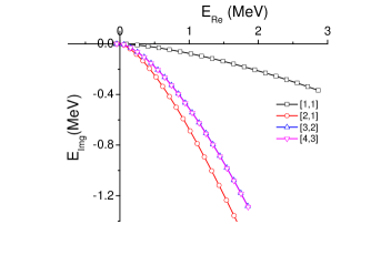
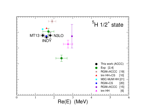
We illustrate in Fig. 3 the ACCC results for the Jπ=1/2+ state with the I-N3LO Hamiltonian. The continuum extrapolation was based on 23 binding energies, starting from the triton threshold MeV up to 300 MeV. Notice that this value – obtained in a 5-body calculation with limited model space – differs only by 0.04 MeV from the fully converged 3-body calculations MeV. Though formally eigenergy entries suffice to determine coeficients of Padé approximant [m,n], as suggested in ref. [18], we have employed much larger eigenenrgy entry sets by determining the coefficient using least-square method. The last trick allows to minimize effect of eigenergy set choice on the convergence of the Padé series as well as reduce the effect of numerical accuracy being finite. Two different parameterizations of potential (5) were considered: =78.4 fm2 and =108.9 fm2, both with .111In our previous work [23] parameterizations with different values of were considered, providing results in agreement with the case; however its implementation requires a more important numerical effort. They correspond respectively to the left- and right-panel of this figure. In both cases, the Padé extrapolation nicely converges to the resonance energy E=1.85(1)-i1.25(5) MeV, a result which is highly ensuring. Nevertheless the convergence relative to the order [m,n] of the Padé approximant should be considered with a grain of salt. Indeed, one could expect that by increasing the order of Padé approximant, the accuracy in the extrapolated energies should improve accordingly. However this expected improvement saturates at order [3,2], when the extrapolated energies are reproduced within 100 keV. This numerical ”saturation” is certainly due to the limited accuracy of the calculated 5-body energy inputs and introduce error bars in our results. In this context, increasing the order of the Padé approximants makes no sense and may even lead to numerical instabilities due to overfitting.
The extraction of the same resonance parameters by means of SECS, provide the value E=1.85(10)-i1.20(5), where errors correspond to the variations of the rotation angle [30,45]∘ and the range parameter [13,16] fm with n=3,4.
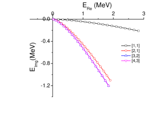
A similar study was performed for the INOY potential. ACCC results, based on parameters =108.9 fm2 were obtained. A Padé extrapolation was constructed from 28 B(5H) binding energies in the interval [8.40,300] MeV. They converge to the value E=1.73(5)-i1.19(9) MeV while SECS provides this resonance at E=1.8(1)-i1.2(1) MeV.
Results for the Jπ=1/2+ ground state of 5H, with different interactions222MT13 results with ACCC method were presented in [23] and the two different methods (ACCC and SECS) used to access complex energies, are summarized in Table 2. As one can see, both methods provide resonance positions and widths compatible within the estimated errors. The width of this state turns out to be almost independent of the employed interaction model – including the semi-realistic MT13 – around a value MeV; its real part seems to be less stable. In particular for MT13 potential real energy of the resonant state seems to be slightly smaller than ones provided by the realistic Hamiltonians. Apparently this might also be the reason for larger deviation between the ACCC and SECS predictions – one has increasing difficulty to calculate accurately resonant states once ratio increases. For J=3/2+ state we were able to get stable results only for MT13 potential and using SECS. As it was the case for 4H, the J=3/2+ and J=5/2+ states resulting from L=2 and total spin S=1/2 coupling, are degenerate due to the absence of spin-orbit and tensor terms within this model.
| J=1/2+ | J=3/2+ | J=5/2+ | ||||
| N3LO (ACCC) | 1.8(1) | 2.4(2) | ||||
| (SECS) | 1.9(2) | 2.4(2) | ||||
| INOY (ACCC) | 1.7(1) | 2.4(2) | ||||
| (SECS) | 1.8(1) | 2.4(2) | ||||
| MT13 (ACCC) | 1.4(1) | 2.4(2) | ||||
| (SECS) | 1.7(2) | 2.4(2) | 2.5(2) | 3.8(4) | 2.5(2) | 3.8(4) |
| [6] tnn | 2.75(25) | 3.5(5) | 6.6(3) | 8 | 4.8(2) | 5 |
| [15] RGM | 3.1(1) | 2.5(15) | ||||
| [20] RGM | 1.59 | 2.48 | 3.0 | 4.8 | 2.9 | 4.1 |
| [10] tnn | 1.57 | 1.53 | 3.25 | 3.89 | 2.82 | 2.51 |
| [21] RGM | 1.39 | 1.60 | 2.11 | 2.87 | 2.10 | 3.14 |
| [19] RGM | 1.9 (2) | 0.6(2) | 4(1) | 3(1) | ||
| Exp. [2] | 1.70.3 | 1.90.4 | ||||
| Exp. [4] | 2.40.3 | 5.30.4 |
Our results are compared with previous calculations. Refs [6] and [10] are based on a 3-body t-n-n approximation with an adjusted t-n two-body potential and an ad-hoc 3-body force, while Refs. [15], [20], [21] and [19] attempt a microscopic calculation assuming a 3H+n+n cluster wave function, properly antisymmetrized. Notice that these model calculations display much larger fluctuations among them than our ab initio results with different potentials.
It is worth noticing that the lowest resonant state of 4H is significantly wider, i.e. has larger width, than the 5H one. This suggest that the 4n system is less repulsive than the 3n one, and contributes in this way to stabilize the 5H isotope with respect to 4H. If this ”pairing tendency” is pursued with one can indeed expect that 7H would be a narrower resonant state than 5H in agreement with GANIL’s 2007 findings, where a ground state of 7H is predicted with the astonishing resonance parameters =0.57 MeV and =0.09 MeV. Conclusions from the recent measurement performed at RIKEN with SAMURAI multineutron detector are expected with interest.
For completeness we have also added in Table 2, the last two experimental results from Refs. [2] and [4]. The results of [2] are fully compatible with our calculations, although, as we have already emphasized, any direct comparison between experiments and theory is not very meaningful, apart from denoting the existence of the same S-matrix pole.
In order to allow the easiest comparison of the ensemble of results of Tables 1 and 2 we have plotted in Fig. 4 the corresponding complex energy values (we recall that ). Left panel corresponds to the three lowest 4H states and right panel to the J=1/2 one in 5H. Our ab initio results are denoted by filled black dots (). Those based on a microscopic 3-cluster calculations the same NN interaction are denoted by colored squares and those based on a 3-body t-n-n description by triangle up symbols. The energy scales have been taken the same in both figures to compare the proximity of 5H and 4H resonances to the physical (real energy) axis and their potential impact on physical observables. The relative stability of 5H with respect to 4H is clearly manifested. Notice that by comparing only the values of these two isotopes, that is forgetting their imaginary part, we could have reached an opposite conclusion. As one can see in this figure, there is quite a large dispersion of the results, even among the microscopic approaches. The positions extracted from the experimental data [44, 2, 4] are indicated by filled green circles.
In the 4H case, the R-matrix analysis systematically predicts resonances parameters larger than our theoretical values which, as well recognized in ref.[44], is quite a common feature when dealing with broad resonant states. This trend is a clear consequence of two approaches having different goals: the S-matrix approach tries to dtermine the analytical properties of the underlying Hamiltonian, whereas the R-matrix analysis attempts to describe the experimental observables with the smallest number of parameters. In the 5H case, since the resonant states turn to be narrower and more pronounced, one might expect a better agreement between the theoretically calculated S-matrix pole positions and the values extracted from the experimental data. Indeed the results from [2] agrees well with our calculated S-matrix poles, while those of [4] provide significantly larger values - similar to the mismatch provided by the R-matrix analysis in the 4H case.
To conclude this section we would like to point out that the methods we have used in this work to compute the resonant position of 5H are strictly the same as those used in our previous studies on the and systems [32, 33, 34, 35, 36] where we refuted the existence of any experimentally meaningful resonant state.
4 Conclusion
We have presented the first ab initio calculation to determine the positions of 5H resonant states. This has been achieved by solving 5-nucleon Faddeev-Yakubovsky equations in configuration space based on realistic nucleon-nucleon interaction models.
Two independent methods were used to locate the resonance positions in the complex energy plane: a variant of the smooth exterior complex scaling method and the analytic continuation on the coupling constant. The results show a remarkable stability with respect to the different tested interactions and support the recent experimental findings [2, 4], although the direct comparison is biased due to the reaction mechanism involved in each experiment and to the indirect way the resonance parameters are extracted.
The resonance parameters of the Jπ=2-,0-,1- states in 4H, which dominate the low-energy n-3H elastic cross section, have been also computed and found to be slightly wider than the ones for 5H ( 4 MeV for MeV) advocating presence of additional attraction of the 4n with respect to 3n system. In view of that, any attempt to reproduce the 7H narrow state would be of the highest interest.
Aknowledgements
Authors are indebted to F. M. Marques for his careful reading of the manuscript and for useful discussions concerning the experimental results. We were granted access to the HPC resources of TGCC/IDRIS under the allocation 2018-A0030506006 made by GENCI (Grand Equipement National de Calcul Intensif). This work was supported by french IN2P3 for a theory project ”Neutron-rich light unstable nuclei” and by the japanese Grant-in-Aid for Scientific Research on Innovative Areas (No.18H05407).
References
- [1] P.G. Young et al., Phys. Rev. 173 (1968) 949.
- [2] A.A. Korsheninnikov, et al., Phys. Rev. Lett. 87 (2001) 092501.
- [3] M.S. Golovkov et al, Phys. Lett. B 566 (2003) 70, Phys. Rev. Lett. 93 (2004) 262501, Phys. Rev. C 72 (2005) 064612.
- [4] A.H. Wuosmaa et al Phys. Rev. C 95 (2017) 014310.
- [5] M. Caamaño et al., Phys. Rev. Lett. 99 (2007) 062502.
- [6] N.B. Shul’gina B.V. Danilin, L.V. Grigorenko, M.V. Zhukov, J.M. Bang, Phys. Rev. C 62 (2000) 014312.
- [7] L.V. Grigorenko et al., Phys. Rev. C 57 (1998) R2099; 60 (1999) 044312.
- [8] D. Gogny, P. Pires, and R. de Tourreil, Phys. Lett. B 32 (1970) 591.
- [9] L.V. Grigorenko, N.K. Timofeyuk, and M.V. Zhukov, Eur. Phys. J. A 19, (2004) 187.
- [10] R. de Diego, E. Garrido, D.V. Fedorov, A.S. Jensen, Nucl. Phys. A 786 (2007) 71.
- [11] E. Garrido, D.V. Fedorov, A.S. Jensen, Phys. Rev. C 69 (2004) 024002.
- [12] E. Hiyama, S. Ohnishi, M. Kamimura, Y. Yamamoto, Nucl. Phys. A 908 (2013) 29.
- [13] R. B. Wiringa, V.G.J. Stoks and R. Schiavilla, Phys. Rev. C 51 (1995) 38.
- [14] N.B. Schul’gina, B.V. Danilin, V.D. Efros, J.S. Baagen, M.V. Zhukov, Nucl. Phys. A 597 (1996) 197.
- [15] P. Descouvemont and A. Kharbach, Phys. Rev. C 63 (2001) 027001.
- [16] D. R. Thompson, M. LeMere, and Y. C. Tang, Nucl. Phys. A 286 (1977) 53.
- [17] T. Mertelmeier and H.M. Hofmann, Nucl. Phys. A 459 (1986) 387.
- [18] V.I. Kukulin, V.M. Krasnopolsky, J. Horc̀ek, Theory of Resonances, Kluwer, Dordrecht (1989).
- [19] A. Adahchour, P. Descouvemont, Nucl. Phys. A 813 (2008) 252.
- [20] Koji Arai, Phys. Rev. C 68 (2003) 034303.
- [21] F. Arickx, J. Broeckhove, V. Vasilevsky, J. of Phys. Conf. Series 111 (2008) 012056.
- [22] A. Hasegawa and S. Nagata, Prog. Theor. Phys. 45 (1971) 786.
- [23] R. Lazauskas, Few-Body Syst. (2018) 59:13; doi.org/10.1007/s00601-018-1333-7.
- [24] R. Lazauskas, Phys. Rev. C 97 (2018) 044002.
- [25] F.M. Marqués et al., RIBF Experimental Proposal NP1512-SAMURAI34.
- [26] O.A. Yakubovsky, Sov. J. Nucl. Phys. 5 (1967) 937.
- [27] L.D. Faddeev, JETP 39 (1960) 1459.
- [28] A. Nogga, H. Kamada, and W. Gloeckle Phys. Rev. Lett. 85 (2000) 944.
- [29] R. Lazauskas and J. Carbonell, Phys. Rev. C 70 (2004) 044002.
- [30] A. Deltuva and A. C. Fonseca, Phys. Rev. C 76 (2007) 021001(R).
- [31] D. Baye, Phys. Rep. 565 (2015) 1.
- [32] R. Lazauskas and J. Carbonell, Phys. Rev. C 71 (2005) 044004.
- [33] R. Lazauskas and J. Carbonell, Phys. Rev. C 72 (2005) 034003.
- [34] E. Hiyama, R. Lazauskas, J. Carbonell, N. Kamimura, Phys. Rev. C 93 (2016) 044004.
- [35] J. Carbonell, R. Lazauskas, E. Hiyama, M. Kamimura, Few-Body Syst. 58, 2 (2017) 58.
- [36] R. Lazauskas, E. Hiyama, J. Carbonell, Prog. Theor. Exp. Phys. 7 (2017) 073D03.
- [37] R. Lazauskas, J. Carbonell, Phys. Rev. C 84 (2011) 044002; Few-Body Syst. 54 (2013) 967.
- [38] B. Simon, Phys. Lett. A 71 (1979) 211.
- [39] D.R. Entem and R. Machleidt, Phys. Rev. C 68 (2003) 041001.
- [40] M. Viviani, et al., Phys. Rev. C 84 (2011) 054010.
- [41] P. Doleschall, Phys. Rev. C 69 (2004) 054001.
- [42] R.A. Malfliet and J.A. Tjon, Nucl. Phys. A127 (1969) 161.
- [43] R. Lazauskas PhD, [http://tel.ccsd.cnrs.fr/documents/archives0/00/00/41/78/], University J. Fourier, Grenoble, 2003.
- [44] D.R. Tilley, H.R. Weller, G.M. Hale, Nucl. Phys. A 541 (1992) 1.