Quasiparticle Band Structure and Spin Excitation Spectrum of the Kondo Lattice

Abstract

A formulation of the Kondo lattice Hamiltonian in terms of bond particles is derived and solved in two different approximations. The bond particles correspond to the eigenstates of a single unit cell and are bosons for states with even electron number and fermions for states with an odd electron number. As a check various physical quantities are calculated for the 1D Kondo insulator and good agreement with numerical results is obtained for $J/t>1$.

I Introduction

Metallic compounds containing Cerium, Ytterbium or Uranium - the so-called Heavy fermions - continue to be a much studied field of solid state physics. These materials show a number of remarkable phenomena which are widely believed to be caused by the strong Coulomb repulsion between the electrons in the $4f$-shells of Cerium and Ytterbium or the $5f$-shell of Uranium. A long known phenomenon is the crossover from a lattice of localized $f$ electrons coexisting with weakly or moderately correlated conduction electron bands at high temperature, to an exotic Fermi liquid with strongly correlation-enhanced effective masses at low temperature, whereby the $f$ electrons now contribute to the Fermi-surface volumeStewart ; kondoinsulators . The low temperature Fermi-liquid phase can undergo magnetic ordering transitions whereby the transition temperature often can be tuned to zero by external parameters such as temperature, pressure, magnetic field or alloying, resulting in quantum critical points and the ensuing non-Fermi-liquid behavior and superconducting domesStewartII ; loenireview ; Steglichreview . An intriguing feature thereby is the fact that whereas the $f$ electrons do contribute to the Fermi surface volume in the paramagnetic phase they seem to ‘drop out’ of the Fermi-surface volume at some of these transitions.
Heavy fermion compounds can be described by the Kondo-lattice model (KLM). In the simplest case of no orbital degeneracy each unit cell $n$ contains one $f$ orbital and one conduction band orbital, and denoting the creation operators for electrons in these orbitals by $f_{n,\sigma}^{\dagger}$ and $c_{n,\sigma}^{\dagger}$ the Kondo lattice Hamiltonian is $H=H_{t}+H_{J}$ with

$$H_{t} = \sum_{m,n}\;\sum_{\sigma}\;t_{m,n}\;c_{m,\sigma}^{\dagger}c_{n,\sigma},$$

$$H_{J} = \sum_{n}\;h_{n},$$

$$h_{n} = J\;\bm{S}_{n,f}\cdot\bm{S}_{n,c},$$

$$\bm{S}_{n,c} = \frac{1}{2}\;\sum_{\sigma,\sigma^{\prime}}\;c_{n,\sigma}^{\dagger}\;\bm{\tau}_{\sigma,\sigma^{\prime}}\;c_{n,\sigma^{\prime}}.$$ (1)

Here $\bm{\tau}$ denotes the vector of Pauli matrices (an analogous definition holds for $\bm{S}_{n,f}$). An important feature of the KLM is the constraint to have precisely one electron per $f$ orbital:

$$\sum_{\sigma}\;f_{n,\sigma}^{\dagger}f_{n,\sigma} = 1,$$ (2)

which must hold separately for each $n$. In the following we consider a lattice with $N$ unit cells and $N_{c}$ conduction electrons. The KLM can be derived from the more realistic periodic Anderson model (PAM) by means of the Schrieffer-Wolff transformationSchriefferWolff .
The impurity versions of the Kondo and Anderson model are well understood. Approximate solutions can be obtained by variational wave functionsYosida ; Varma ; Gu , mean-field (or saddle point) approximation to the exchange termYoshimoriSakurai ; ReadNewns , or Green’s function techniques where the hybridization or exchange between the $f$ level and conduction band are treated as perturbationKeiter ; Kuramoto ; Coleman . Thereby the inverse of the degeneracy $n_{f}$ of the $f$ level, $1/n_{f}$, often plays the role of a small parameterBickers . Exact solutions of the impurity models can be obtained by renormalization groupRG and Bethe ansatzBethe . The ground state of the impurity is a singlet formed from the $f$ electron on the impurity and an extended screening state formed from the conduction band states, whereby for weak coupling ($J\ll t$) the binding energy - the so-called Kondo temperature - is $k_{B}T_{K}\propto We^{-\frac{1}{\rho J}}$. Here $W$ and $\rho$ are bandwidth and density of states of the conduction band.
The lattice versions of the model are less-well understood. A noteworthy result is the fact that even for the KLM, where the $f$ electrons are strictly localized, they do contribute to the Fermi surface volumeOshikawa provided the system is a Fermi liquid. Approximate results for the KLM and PAM have been obtained in the mean-field (or saddle-point) approximation. For the KLM the exchange term, which is quartic in electron operators is factorizedLacroixCyrot ; Lacroix ; AuerbachLevin ; Burdinetal ; ZhangYu ; Lavagna ; Senthil ; Global ; ZhangSuLu ; Nilsson ; Montiel , whereas for the PAM a slave-boson representation is usedMillisLee ; ReadNewns1 . The models also have been studied using Gutzwiller-type trial wave functionsRiceUeda ; Fazekas . The resulting band structure is consistent with a simple hybridization picture: a dispersionless effective $f$ band close to the Fermi energy of the decoupled conduction band hybridizes with the conduction electron band via an effective hybridization matrix element $\propto k_{B}T_{K}$ at weak coupling. This results in a Fermi surface with a volume corresponding to itinerant $f$ electrons and the ‘heavy bands’ characteristic of heavy fermion compounds. In addition to mean-field theories, a large amount of quantitative results has also been gathered by numerical methods such as Density Matrix Renormalization Group (DMRG)yuwhite ; MC1 ; MC2 ; Mutou ; Smerat , Dynamical Mean-Field (DMFT) calculationsJ1 ; J2 ; J3 ; peterspruschke , Quantum Monte-Carlo (QMC)Carsten ; Assaad , series expansion (SE)series ; seriesexp ; Trebst , Variational Monte-Carlo (VMC)WatanabeOgata ; Asadzadeh ; Kubo , exact diagonalizationTsunetsugu ; White ; Tsutsui , Dynamical Cluster ApproximationMartinAssaad ; MartinBerxAssaad and Variational Cluster ApproximationLenz . For the paramagnetic phase the numerical techniques produce band structures which are consistent with the hybridization picture, whereby it has to be kept in mind that numerical methods often have problems to access the limit of small $J/t$ and thus to reproduce the Kondo scale $k_{B}T_{K}$. However, the heavy quasiparticles and the fact that the $f$ electrons do participate to the Fermi surface in the KLM and PAM are reproduced.
Considerable effort was devoted to a study of the magnetic phase transitions which are believed to be due to a competitionDoniach between the singlet formation in the impurity model and the RKKY-interaction between the $f$ spinsRKKY mediated by the conduction electrons. A controversial question is whether the heavy quasiparticles persist at the magnetic transition, so that this may be viewed as the heavy Fermi liquid undergoing a conventional spin-density-wave transition, or whether the magnetic ordering suppresses the heavy Fermi liquid alltogether. Numerous studies have addressed magnetic orderingK1 ; K2 ; K3 ; K4 ; K5 ; K6 ; K7 ; K8 ; K9 ; K10 ; K11 ; K12 ; K13 but open questions remain.
It is the purpose of the present manuscript to present a theory for the single-particle band structure and spin excitation spectrum of the Kondo lattice which relies on the interpretation of the eigenstates of a single cell as fermionic or bosonic particles, which we call bond particles. Bond particle theory was proposed originally by Sachdev and BhattSachdevBhatt to study spin systems and applied to spin laddersGopalan , bilayersvojta1 ; vojta2 , intrisically dimerized spin systemssushkov ; Park and the ‘Kondo necklace’Siahatgar . It was also applied to the PAMOana , as well as antiferromagnetic (AF) ordering in the planar KLMJureckaBrenig ; KotovHirschfeld , a discussion of its different AF phasesafbf and the band structure in the AF phaseafbf1 . It is by nature a strong-coupling theory which should work best in the (unphysical) limit of $J/t\gg 1$. However, as will be shown below by comparison to numerical results, there is some reason to hope that the theory retains its validity down to $t/J\approx 1$ which may be sufficient to discuss magnetic ordering phenomena.

II Hamiltonian

We consider eigenstates of the single cell exchange term $h_{n}$. Introducing the matrix $4$-vector $\bm{\gamma}=(\tau_{0},\bm{\tau})$ with $\tau_{0}=1$ the state $4$-vector $\bm{\beta}_{n}=(s_{n},\bm{t}_{n})$ isSachdevBhatt ; Gopalan

$$|\bm{\beta}_{n}\rangle=\frac{1}{\sqrt{2}}\;\sum_{\sigma,\sigma^{\prime}}\;c_{n,\sigma}^{\dagger}\;(\bm{\gamma}i\tau_{y})_{\sigma,\sigma^{\prime}}\;f_{n,\sigma^{\prime}}^{\dagger}|0\rangle.$$ (3)

These are the singlet ($|s_{n}\rangle$) with energy $-\frac{3J}{4}$ and the three components of the triplet ($|\bm{t}_{n}\rangle$) with energy $\frac{J}{4}$.
The single-cell states with an odd number of electrons (which have energy $0$) are

$$|a,n,\sigma\rangle = f_{n,\sigma}^{\dagger}|0\rangle,$$

$$|b,n,\sigma\rangle = c_{n,\uparrow}^{\dagger}c_{n,\downarrow}^{\dagger}f_{n,\sigma}^{\dagger}|0\rangle.$$ (4)

We now rewrite the KLM as a Hamiltonian for bosons and fermions which correspond to these single-cell eigenstates. More precisely, if a given cell $n$ is in one of the states (3) with $2$ electrons we consider it as occupied by a boson, created by the respective operator $4$-vector $(s_{n}^{\dagger},\bm{t}_{n}^{\dagger})$ whereas if it is in one of the states (4) with a single (three) electrons we consider it as occupied by a fermion created by $a_{n,\sigma}^{\dagger}$ ($b_{n,\sigma}^{\dagger}$). The latter correspond to the ‘bachelor spins’ in the $U/t=\infty$ Hubbard model to which the KLM reducesNozieres for $J/t\rightarrow\infty$ and $N_{c}\neq N$.
In order for this representation to make sense each cell must be occupied by precisely one of these particles resulting in the constraint (to be obeyed for each $n$)

$$s_{n}^{\dagger}s_{n}+\sum_{\sigma}\left(\;a_{n,\sigma}^{\dagger}a_{n,\sigma}+b_{n,\sigma}^{\dagger}b_{n,\sigma}\right)+\bm{t}_{n}^{\dagger}\cdot\bm{t}_{n}=1.$$ (5)

On the other hand, each of the basis states (3) and (4) obeys the constraint (2) exactly, so that this constraint is ‘built in’ into the theory. In terms of the bond particles the exchange term is

$$H_{J} = \sum_{n}\;\left(\;\frac{3J}{4}\sum_{\sigma}\;(b_{n,\sigma}^{\dagger}b_{n,\sigma}+a_{n,\sigma}^{\dagger}a_{n,\sigma})+J\;\bm{t}_{n}^{\dagger}\cdot\bm{t}_{n}\;\right)$$ (6)

$$\;\;\;\;\;\;\;\;\;\;\;\;\;\;\;\;\;\;\;\;\;\;\;\;\;\;\;\;\;\;\;\;-\frac{3NJ}{4}.$$

On the other hand, we might also write

$$H_{J} = \sum_{n}\;\left(\;-\frac{3J}{4}\;s_{n}^{\dagger}s_{n}+\frac{J}{4}\;\bm{t}_{n}^{\dagger}\cdot\bm{t}_{n}\;\right).$$ (7)

As long as the constraint (5) holds these two forms are equivalent - we wil continue to use (6). From now on we take a fermion operator with omitted spin index to denote a two-component column vector, e.g.

$$c_{n} = \left(\begin{array}[]{c}c_{n,\uparrow}\\ c_{n,\downarrow}\end{array}\right).$$

In this notation the representation of the electron annihilation operator in terms of the bond particles is

$$c_{n}=\frac{1}{\sqrt{2}}\;:\left(\;(s_{n}+{\bm{t}}_{n}\cdot{\bm{\tau}})\;i\tau_{y}a_{n}^{\dagger}-(s_{n}^{\dagger}-{\bm{t}}_{n}^{\dagger}\cdot{\bm{\tau}})\;b_{n}\;\right):$$

(9)

where $:\dots:$ denotes normal ordering. Up to the numerical prefactors the form of this equation follows from the requirement that both sides be covariant spinors and the fact that ${\bm{t}}$ and ${\bm{t}}^{\dagger}$ are vector operators. The representation of the kinetic energy $H_{t}$ is obtained by substituting (9) into (1). One obtains $H_{t}=H_{1}+H_{2}+H_{3}+H_{4}$ with

$$H_{1} = \sum_{m,n}\;\frac{t_{m,n}}{2}\;\sum_{\sigma}\;\left(\;b_{m,\sigma}^{\dagger}b_{n,\sigma}-a_{m,\sigma}^{\dagger}a_{n,\sigma}\;\right)\;s_{n}^{\dagger}\;s_{m}-\sum_{m,n}\;\frac{t_{m,n}}{2}\;\left[\;\left(\;b_{m,\uparrow}^{\dagger}a_{n,\downarrow}^{\dagger}-b_{m,\downarrow}^{\dagger}a_{n,\uparrow}^{\dagger}\;\right)\;s_{m}\;s_{n}+H.c.\;\right],$$

$$H_{2} = \sum_{m,n}\;\frac{t_{m,n}}{2}\;\sum_{\sigma}\;\left(\;b_{m,\sigma}^{\dagger}b_{n,\sigma}-a_{m,\sigma}^{\dagger}a_{n,\sigma}\;\right)\;\bm{t}_{n}^{\dagger}\cdot\bm{t}_{m}\;+\sum_{m,n}\;\frac{t_{m,n}}{2}\;\left[\;\left(\;b_{m,\uparrow}^{\dagger}a_{n,\downarrow}^{\dagger}-b_{m,\downarrow}^{\dagger}a_{n,\uparrow}^{\dagger}\;\right)\bm{t}_{m}\cdot\bm{t}_{n}\;+H.c\;\right],$$

$$H_{3} = -\;\sum_{m,n}\;\frac{t_{m,n}}{2}\;\left[\;\left(\;{\bm{\pi}}^{\dagger}_{m,n}\cdot\left(\;s_{m}\;\bm{t}_{n}-\bm{t}_{m}\;s_{n}\right)+H.c.\;\right)+\left(\;\bm{b}_{m,n}-\bm{a}_{m,n}\;\right)\cdot(\bm{t}_{n}^{\dagger}\;s_{m}+s_{n}^{\dagger}\;\bm{t}_{m}\;)\;\right],$$

$$H_{4} = \sum_{m,n}\;\frac{t_{m,n}}{2}\;\left[\;\left[\;i{\bm{\pi}}^{\dagger}_{m,n}\cdot(\;\bm{t}_{m}\times\bm{t}_{n}\;)+H.c.\;\right]-i\;(\;\bm{b}_{m,n}-\bm{a}_{m,n}\;)\cdot(\;\bm{t}_{n}^{\dagger}\times\bm{t}_{m}\;)\;\right],$$ (10)

with the following vectors formed from the fermions:

$$\bm{b}_{m,n} = \sum_{\sigma,\sigma^{\prime}}\;b_{m,\sigma}^{\dagger}\;\bm{\tau}_{\sigma,\sigma^{\prime}}\;b_{n,\sigma^{\prime}},$$

$$\bm{a}_{m,n} = \sum_{\sigma,\sigma^{\prime}}\;a_{m,\sigma}^{\dagger}\;\bm{\tau}_{\sigma,\sigma^{\prime}}\;a_{n,\sigma^{\prime}},$$

$$\bm{\pi}^{\dagger}_{m,n} = \sum_{\sigma,\sigma^{\prime}}\;b_{m,\sigma}^{\dagger}\;\left(\bm{\tau}\;i\tau_{y}\right)_{\sigma,\sigma^{\prime}}\;a_{n,\sigma^{\prime}}^{\dagger}.$$

Strictly speaking the individual terms in this Hamiltonian have to be ‘site-wise normal ordered’ e.g. $b_{m,\sigma}^{\dagger}b_{n,\sigma}t_{n,\alpha}^{\dagger}t_{m,\alpha}\rightarrow b_{m,\sigma}^{\dagger}t_{m,\alpha}t_{n,\alpha}^{\dagger}b_{n,\sigma}$ but since this normal ordering always involves commutation of a fermion and a boson neither nonvanishing commutators nor Fermi signs will arise. The number of electrons - including the localized $f$ electrons - in the system is

$$N_{e} = 2\;\sum_{n}\;(\;s_{n}^{\dagger}s_{n}+\bm{t}_{n}^{\dagger}\cdot\bm{t}_{n}\;)$$ (11)

$$\;\;\;\;\;\;\;\;\;\;\;\;\;\;\;\;+\sum_{n,\sigma}\left(\;3\;b_{n,\sigma}^{\dagger}b_{n,\sigma}+a_{n,\sigma}^{\dagger}a_{n,\sigma}\right)$$

$$= 2N+\sum_{n}\;\sum_{\sigma}\left(\;b_{n,\sigma}^{\dagger}b_{n,\sigma}-a_{n,\sigma}^{\dagger}a_{n,\sigma}\right)$$

$$= \sum_{n}\;\sum_{\sigma}\left(\;b_{n,\sigma}^{\dagger}b_{n,\sigma}+a_{n,\sigma}a_{n,\sigma}^{\dagger}\;\right),$$

where (5) was used to obtain the second line. The Hamiltonian (6)$+$(10) together with the constraint (5) provides an exact representation of the KLM. On the other hand, it is compliated and impossible to solve even approximately e.g. by diagrammatic methods, due to the constraint (5), which is equivalent to an infinitely strong Hubbard-like repulsion between the bond particles. The whole formulation in terms of bond particles will be useful only if we can identify the fermions and triplet bosons as approximate quasiparticles and spin excitations of the system and find a way to extract a sufficiently simple yet accurate theory for these. A considerable simplification becomes possible by making use of the fact - to be verified below - that over large regions of parameter space the densities of fermions and triplets are relatively small so that the vast majority of cells is in the singlet state. Thus, if one can get rid of the singlets by either considering them as condensed or by re-interpreting the singlet as the ‘true vacuum state’ of a cell, one retains a theory for a system of fermions and bosons which in principle are still subject to the infinitely strong repulsion implied by the constraint (5) but which have a low density so that relaxing the constraint may be a reasonable approximation. Put another way, by using the bond particles one can trade the constraint (2) which refers to a dense system of electrons - the density of $f$ electrons is 1/cell - for a constraint like (5) without singlets which refers to a system of particles with a relatively low density. In the following, we explore two possible approximation schemes to ‘get rid of the singlets’ and compare the results to numerical calculations. It should also be noted that while we will not do so in the following, it is in principle possible to deal with strong repulsion in a low density system by well-known field theoretical methodsFW . For the case of bond bosons in spin systems this has in fact been carried out explicitely by Kotov et al.Kotov and Shevchenko et al.Shevchenko . We will compare the results from bond particle theory to numerical results for the paramagnetic state in a one-dimensional chain with only nearest neighbor hopping $-t$ and $n_{e}=2$ - i.e. the 1D Kondo insulatoruedareview , throughout $t$ is the unit of energy.

III Mean Field Theory

As a first approximation we study the Hamiltonian in mean-field approximation. This approximation was applied previously to spin systemsSachdevBhatt ; Gopalan and to antiferromagnetic ordering in the planar KLMJureckaBrenig . Since we are interested in the paramagnetic phase we initially drop the terms $H_{3}$ and $H_{4}$. $H_{3}$ describes pair creation and propagation processes whereby a single triplet-boson is absorbed or emitted. In mean-field theory this term would contribute only in a state where the triplets are condensedJureckaBrenig i.e. a magnetically ordered stateSachdevBhatt . Similarly, $H_{4}$ describes pair creation and propagation processes whereby two triplets coupled to a vector are emitted/absorbed. The resulting vector-like order parameters would be important to describe a state with incommensurate or spiral magnetic order but vanish in a rotationally invariant state.
In the remaining terms $H_{J}+H_{1}+H_{2}$ the singlets are assumed to be condensed whence the corresponding operators can be replaced by a real number, $s_{n}^{\dagger},s_{n}\rightarrow s$. The condensation amplitude $s$ now is a freely variable internal parameter of the system, to be determined by minimization of the Helmholtz free energy. The constraint (5) is replaced by the global constraint

$$\sum_{n}\;\left(\;s^{2}+\bm{t}_{n}^{\dagger}\cdot\bm{t}_{n}+\sum_{\sigma}(b_{n,\sigma}^{\dagger}b_{n,\sigma}+a_{n,\sigma}^{\dagger}a_{n,\sigma})\;\right) = N.$$

We perform a Hartree-Fock factorization of the quartic terms in $H_{2}$ and add the constraints (LABEL:constraint_g) and (11) using the Lagrange multipliers $\lambda$ and $\mu$, respectively. We call the resulting Hamiltonian $H_{MF}$ and have $H_{MF}=H_{F}+H_{B}+Nc$. The fermionic Hamiltonian is

$$H_{F} = e_{0}\;\sum_{n,\sigma}\;\left(\;b_{n,\sigma}^{\dagger}b_{n,\sigma}+a_{n,\sigma}^{\dagger}a_{n,\sigma}\;\right)$$

$$\;\;+\sum_{m,n}\;\tilde{t}_{m,n}\;\sum_{\sigma}\;\left(\;b_{m,\sigma}^{\dagger}b_{n,\sigma}-a_{m,\sigma}^{\dagger}a_{n,\sigma}\;\right)$$

$$\;\;\;\;-\sum_{m,n}\;\left[\Delta_{m,n}\;\left(\;b_{m,\uparrow}^{\dagger}a_{n,\downarrow}^{\dagger}-b_{m,\downarrow}^{\dagger}a_{n,\uparrow}^{\dagger}\;\right)+H.c.\right]$$

$$\;\;\;\;-\mu\;\sum_{n,\sigma}\;\left(\;b_{n,\sigma}^{\dagger}b_{n,\sigma}+a_{n,\sigma}a_{n,\sigma}^{\dagger}\;\right)$$

where $e_{0}=\frac{3J}{4}-\lambda$ and

$$\tilde{t}_{m,n} = \frac{t_{m,n}}{2}s^{2}+\zeta_{m,n}$$

$$\Delta_{m,n} = \frac{t_{m,n}}{2}s^{2}+\eta_{m,n}.$$

with $\zeta_{m,n}=\frac{t_{m,n}}{2}\;\langle\bm{t}_{n}^{\dagger}\cdot\bm{t}_{m}\;\rangle$, $\eta_{m,n}=-\frac{t_{m,n}}{2}\;\langle\bm{t}_{m}\cdot\bm{t}_{n}\;\rangle$. We consider a translationally invariant and isotropic state and accordingly assume that expectation values such as $\zeta_{m,n}$ depend only on $|\bm{R}_{m}-\bm{R}_{n}|$ so that

$$H_{F} = e_{0}\;\sum_{\bm{k},\sigma}\;\left(\;b_{\bm{k},\sigma}^{\dagger}b_{\bm{k},\sigma}-a_{-\bm{k},\bar{\sigma}}a_{-\bm{k},\bar{\sigma}}^{\dagger}\;\right)$$

$$+\sum_{\bm{k},\sigma}\;(\tilde{t}_{\bm{k}}-\mu)\left(\;b_{\bm{k},\sigma}^{\dagger}b_{\bm{k},\sigma}+a_{-\bm{k},\bar{\sigma}}a_{-\bm{k},\bar{\sigma}}^{\dagger}\;\right)$$

$$\;\;\;\;\;\;\;\;-\sum_{\bm{k},\sigma}\;sign(\sigma)(\Delta_{\bm{k}}\;b_{\bm{k},\sigma}^{\dagger}a_{-\bm{k},\bar{\sigma}}^{\dagger}+H.c.)$$

$$\;\;\;\;\;\;\;\;\;\;\;\;\;\;\;\;-\;2\sum_{\bm{k}}\;(\tilde{t}_{\bm{k}}-e_{0}),$$

with the Fourier transform of the hopping integral

$$\tilde{t}_{\bm{k}} = \sum_{\bm{r}}\;e^{i\bm{k}\cdot\bm{r}}\;\tilde{t}_{\bm{r}}$$ (13)

$$= \sum_{\bm{\alpha}}\;z_{\bm{\alpha}}\tilde{t}_{\bm{\alpha}}\gamma_{\bm{\alpha}}({\bm{k}})$$

and an analogous definition of $\Delta_{\bm{k}}$. Here ${\bm{\alpha}}$ denotes shells of symmetry-equivalent neighbors of a given site, $z_{\bm{\alpha}}$ the number of neighbors belonging to a shell, and $\gamma_{\bm{\alpha}}$ the respective tight-binding harmonic. This can be solved by the unitary transformation

$$\alpha_{\bm{k}}^{\dagger} = \;\;\,u_{\bm{k}}\;b_{\bm{k}}^{\dagger}+v_{\bm{k}}\;i\tau_{y}\;a_{-\bm{k}},$$

$$\beta_{\bm{k}}^{\dagger} = -v_{\bm{k}}\;b_{\bm{k}}^{\dagger}+u_{\bm{k}}\;i\tau_{y}\;a_{-\bm{k}},$$ (14)

so that

$$H_{F} = \sum_{\bm{k},\sigma}\;(\;E_{\alpha,\bm{k}}\;\alpha_{\bm{k},\sigma}^{\dagger}\alpha_{\bm{k},\sigma}+E_{\beta,\bm{k}}\;\beta_{\bm{k},\sigma}^{\dagger}\beta_{\bm{k},\sigma}\;)$$

$$\;\;\;\;\;\;\;\;\;\;\;\;\;\;\;\;\;\;\;\;\;\;\;\;\;\;\;\;\;\;\;\;-\;2\sum_{\bm{k}}\;(\tilde{t}_{\bm{k}}-e_{0}).$$

Here $E_{\nu,\bm{k}}=\tilde{t}_{\bm{k}}\pm W_{\bm{k}}-\mu$ and $\alpha$ corresponds to the lower of the two energies. Thereby

$$W_{\bm{k}} = \sqrt{e_{0}^{2}+\Delta_{\bm{k}}^{2}},$$

$$u_{\bm{k}} = -\sqrt{\frac{W_{\bm{k}}-e_{0}}{2W_{\bm{k}}}},$$

$$v_{\bm{k}} = \frac{-\Delta_{\bm{k}}}{\sqrt{2W_{\bm{k}}(W_{\bm{k}}-e_{0})}}.$$

By virtue of the unitarity of (14) it follows that the electron number (11) becomes

$$N_{e} = 2\;\sum_{{\bm{k}},\sigma}\;(\;\alpha_{\bm{k},\sigma}^{\dagger}\alpha_{\bm{k},\sigma}+\beta_{\bm{k},\sigma}^{\dagger}\beta_{\bm{k},\sigma}\;).$$

The volume of the quasiparticle Fermi surface therefore corresponds to both, conduction electrons and $f$ electrons. Despite the fact that all basis states have precisely one $f$ electron per cell, so that these are strictly localized, the $f$ electrons do contribute to the Fermi surface volume as if they were itinerantOshikawa .
The bosonic Hamiltonian is (with $\tilde{J}=J-\lambda$)

$$H_{B} = \tilde{J}\;\sum_{n}\;\bm{t}_{n}^{\dagger}\cdot\bm{t}_{n}+\sum_{m,n}\;\tilde{\zeta}_{m,n}\;\bm{t}_{n}^{\dagger}\cdot\bm{t}_{m}$$

$$\;\;\;\;\;\;\;\;+\sum_{m,n}(\;\tilde{\eta}_{m,n}\;\bm{t}_{m}\cdot\bm{t}_{n}+H.c.),$$

$$\tilde{\zeta}_{m,n} = \frac{t_{m,n}}{2}\;\sum_{\sigma}\;\langle\;b_{m,\sigma}^{\dagger}b_{n,\sigma}-a_{m,\sigma}^{\dagger}a_{n,\sigma}\;\rangle,$$

$$\tilde{\eta}_{m,n} = \frac{t_{m,n}}{2}\;\langle\;b_{m,\uparrow}^{\dagger}a_{n,\downarrow}^{\dagger}-b_{m,\downarrow}^{\dagger}a_{n,\uparrow}^{\dagger}\;\rangle.$$

Fourier transformation gives

$$H_{B} = \sum_{\bm{k}}\;(\tilde{J}+\tilde{\zeta}_{\bm{k}})\;\bm{t}_{\bm{k}}^{\dagger}\cdot\bm{t}_{\bm{k}}+\sum_{\bm{k}}\;(\tilde{\eta}_{\bm{k}}\;\bm{t}_{\bm{k}}\cdot\bm{t}_{-\bm{k}}+H.c.),$$

with $\tilde{\zeta}_{\bm{k}}$ and $\tilde{\eta}_{\bm{k}}$ defined as in (13). This can be solved by the ansatz $\bm{\tau}_{\bm{k}}^{\dagger}=\tilde{u}_{\bm{k}}\;\bm{t}_{\bm{k}}^{\dagger}+\tilde{v}_{\bm{k}}\;\bm{t}_{-\bm{k}}$ and $H_{B}$ becomes

$$H_{B} = \sum_{\bm{k}}\;\omega_{\bm{k}}\;\bm{\tau}_{\bm{k}}^{\dagger}\cdot\bm{\tau}_{\bm{k}}+\frac{3}{2}\;\sum_{\bm{k}}\;(\omega_{\bm{k}}-(\tilde{J}+\tilde{\zeta}_{\bm{k}})).$$

Thereby

$$\omega_{\bm{k}} = \sqrt{(\tilde{J}+\tilde{\zeta}_{\bm{k}})^{2}-4\;\tilde{\eta}_{\bm{k}}^{2}}$$

$$\tilde{u}_{\bm{k}} = \frac{2\tilde{\eta}_{\bm{k}}}{\sqrt{{2\omega_{\bm{k}}(\tilde{J}+\tilde{\zeta}_{\bm{k}}-\omega_{\bm{k}})}}},$$

$$\tilde{v}_{\bm{k}} = \sqrt{\frac{\tilde{J}+\tilde{\zeta}_{\bm{k}}-\omega_{\bm{k}}}{{2\omega_{\bm{k}}}}}.$$

The additive constant is $Nc$ with

$$c = -\frac{3J}{4}+\lambda(1-s^{2})+\mu n_{e}-\Theta,$$

$$\Theta = \sum_{\bm{\alpha}}\;\frac{2z_{\bm{\alpha}}}{t_{\bm{\alpha}}}\;\left(\;\zeta_{\bm{\alpha}}\tilde{\zeta}_{\bm{\alpha}}-2\eta_{\bm{\alpha}}\tilde{\eta}_{\bm{\alpha}}\;\right),$$

and the Helmholtz free energy becomes

$$F = -\frac{2}{\beta}\;\sum_{\bm{k}}\;\sum_{\nu\in\{\alpha,\beta\}}\;\log\left(1+e^{-\beta E_{\nu,\bm{k}}}\right)+\frac{3}{\beta}\;\sum_{\bm{k}}\;\log\left(1-e^{-\beta\omega_{\bm{k}}}\right)-\;2\sum_{\bm{k}}(\tilde{t}_{\bm{k}}-e_{0})+\frac{3}{2}\;\sum_{\bm{k}}\;\left(\omega_{\bm{k}}-(\tilde{J}+\tilde{\zeta}_{\bm{k}})\right)+Nc.$$

Had we used the alternative form (7) for $H_{J}$ we would have obtained the same expression with $\lambda-\frac{3J}{4}\rightarrow\lambda$. Minimizing $F$ with respect to $\lambda$ gives $1-s^{2}-n_{F}-n_{B}=0$ where

$$n_{F} = \frac{1}{N}\sum_{\bm{k},\sigma}\;\langle b_{\bm{k},\sigma}^{\dagger}b_{\bm{k},\sigma}+a_{\bm{k},\sigma}^{\dagger}a_{\bm{k},\sigma}\rangle=\frac{2}{N}\sum_{\bm{k}}\left[1-\frac{e_{0}}{W_{\bm{k}}}\;\left(\;f(E_{\alpha,\bm{k}})-f(E_{\beta,\bm{k}})\;\right)\right],$$

$$n_{B} = \frac{1}{N}\sum_{\bm{k}}\;\langle\bm{t}^{\dagger}\cdot\bm{t}\rangle=\frac{3}{N}\sum_{\bm{k}}\;\left[\frac{\tilde{J}+\tilde{\zeta}_{\bm{k}}}{2\omega_{\bm{k}}}\;\coth\left(\frac{\beta\omega_{\bm{k}}}{2}\right)-\frac{1}{2}\right],$$

are the densities of fermions and bosons, respectively. Minimization with respect to the $\zeta$ and $\eta$ parameters in $H_{F}$ and $H_{B}$ gives the self-consistency equations

$$\zeta_{\bm{\alpha}} = \frac{3t_{\bm{\alpha}}}{2N}\sum_{\bm{k}}\;\gamma_{\bm{\alpha},\bm{k}}\left[\frac{\tilde{J}+\tilde{\zeta}_{\bm{k}}}{2\omega_{\bm{k}}}\coth\left(\frac{\beta\omega_{\bm{k}}}{2}\right)-\frac{1}{2}\right],$$

$$\eta_{\bm{\alpha}} = \frac{3t_{\bm{\alpha}}}{2N}\sum_{\bm{k}}\;\gamma_{\bm{\alpha},\bm{k}}\;\frac{\tilde{\eta}_{\bm{k}}}{\omega_{\bm{k}}}\coth\left(\frac{\beta\omega_{\bm{k}}}{2}\right),$$

$$\tilde{\zeta}_{\bm{\alpha}} = \frac{t_{\bm{\alpha}}}{N}\;\sum_{\bm{k}}\;\gamma_{\bm{\alpha},\bm{k}}\;\left[f(E_{\alpha,\bm{k}})+f(E_{\beta,\bm{k}})-1\right],$$

$$\tilde{\eta}_{\bm{\alpha}} = \frac{t_{\bm{\alpha}}}{N}\;\sum_{\bm{k}}\;\gamma_{\bm{\alpha},\bm{k}}\;\frac{\Delta_{\bm{k}}}{2W_{\bm{k}}}\;\left[\;f(E_{\alpha,\bm{k}})-f(E_{\beta,\bm{k}})\;\right].$$

The above equations can also be derived ‘directly’, by evaluating the respective thermal averages with the bosonic and fermionic mean-field Hamiltonian. Differentiation with respect to $s$ gives the additional condition

$$\lambda = \frac{1}{N}\;\sum_{\bm{k}}\;\epsilon_{\bm{k}}\;\left[\;f(E_{\alpha,\bm{k}})+f(E_{\beta,\bm{k}})-1\;\right]$$

$$\;\;\;\;\;\;\;\;-\frac{1}{N}\;\sum_{\bm{k}}\;\epsilon_{\bm{k}}\;\frac{\eta_{\bm{k}}}{W_{\bm{k}}}\;\left[\;f(E_{\alpha,\bm{k}})-f(E_{\beta,\bm{k}})\;\right],$$

where $\epsilon_{\bf k}$ is the noninteracting dispersion. The resulting set of coupled equations can be solved numerically thereby using Broyden’s algorithmBroyden for better convergence.

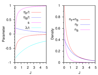
Figure 1: Self-consistent parameters of the mean-field solution versus $J/t$ (Left). Densities of the fermions and bosons versus $J/t$ (Right).

For the Kondo-insulator with nearest-neighbor hopping particle hole-symmetry results in $\zeta_{\bm{k}}=\tilde{\zeta}_{\bm{k}}=0$. Figure 1 shows the remaining parameters, $\eta$, $s$ and $\lambda$ as functions of $J/t$. The parameter $s$ reaches zero for $J_{min}/t\approx 0.1173$ and there is no solution for smaller values of $J/t$. The reason is that even for $s=0$ the parameters $\Delta_{\bm{k}}$ and $\tilde{\eta}$ are finite and in fact increase for small $J/t$ so that the resulting density of particles, $n_{B}+n_{F}$, exceeds $1$ at $J_{min}$ and (5) can no longer be fulfilled. This may be a consequence of the fact that the bond particle formulation of the Kondo lattice ultimately is a strong-coupling theory which is justified best for $J/t\rightarrow\infty$. It should also be noted that once the particle density $n_{B}+n_{F}$ approaches unity, the bond particle theory is highly unreliable anyway.
The mean-field expectation values $\eta_{\bm{k}}$ and $\tilde{\eta}_{\bm{k}}$ are small for $J/t>1$, the parameter $\lambda$ is relatively large and negative.

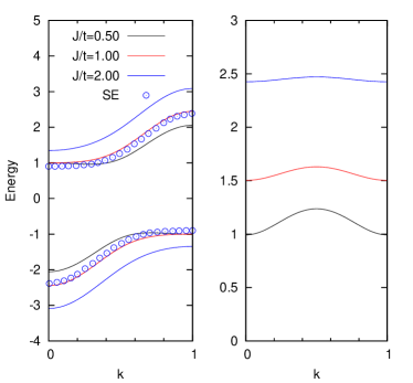
Figure 2: Quasiparticle bands (Left) and triplet frequency (Right) for the 1D Kondo insulator from mean field theory, wave vectors in unit of $\pi$. Data points were obtained by SE for $J/t=2$seriesexp .

Figure 2 shows the bands $E_{\nu,{\bm{k}}}$ for the fermions and the dispersion $\omega_{{\bm{k}}}$ of the bosons. The smallness of $\tilde{\eta}$ results in a small bandwidth for the bosons, whereas the relatively large and negative $\lambda$ results in a large bandgap for the fermions which stays approximately constant for $J/t<1$, as well as a considerable upward shift of the triplet dispersion. The band structure is consisten with the hybridization picture with extended ‘heavy’ band portions and is roughly consistent with numerical results results for the 1D PAMTsutsui ; Carsten and KLMseriesexp although the size of the gap comes out too large. QMC has also shown a well-defined weakly dispersive and gapped mode in the dynamical spin correlation function of the PAMCarsten , roughly consistent with the mean-field boson dispersion. The boson dispersion is symmetric with respect to $k=\frac{\pi}{2}$ whereas DMRG calculations find the maximum of the dispersion of the lowest triplet state at $k=0$, the minimum at $k=\pi$yuwhite . We define the quasiparticle gap, $\Delta_{QP}=E_{0}^{(N+1)}+E_{0}^{(N-1)}-2E_{0}^{(N)}$ which we approximate by the band gap i.e. in 1D $\Delta_{QP}=E_{\beta}(k=0)-E_{\alpha}(k=\pi)$.
So far we have ignored the terms $H_{3}$ and $H_{4}$ because a mean-field treatment of these terms would result in some type of magnetic order. To study the contribution of $H_{3}$ and $H_{4}$ as well as the unfactorized remainder of $H_{2}$ to the ground state energy at least approximately, we treat these terms in 2^nd order perturbation theory in analogy to Møller-Plesset perturbation theoryMP . Since the Kondo insulator has a finite gap in its excitation spectrum this is probably a good approximation. More precisely, we take the mean-field Hamiltonian $H_{MF}=H_{F}+H_{B}+Nc$ as the unperturbed Hamiltonian - its ground state is the product of the ground states of $H_{F}$ and $H_{B}$. The perturbation is

$$\tilde{H}_{1} = H_{2}+H_{3}+H_{4}-(H_{2,MF}-N\Theta)$$

where $H_{2,MF}$ is the mean-field factorized form of $H_{2}$ i.e. the terms in $H_{F}+H_{B}$ which are $\propto\eta,\zeta,\tilde{\eta},\tilde{\zeta}$. $\tilde{H}_{1}$ thus is a sum of terms of the form

$$\sum_{m,n}\frac{t_{m,n}}{2} \left(\;O_{m,n}^{(F)}\;O_{m,n}^{(B)}-O_{m,n}^{(F)}\;\langle O_{m,n}^{(B)}\rangle\right.$$

$$\left.\;\;\;\;\;\;\;\;-\langle O_{m,n}^{(F)}\rangle\;O_{m,n}^{(B)}+\langle O_{m,n}^{(F)}\rangle\;\langle O_{m,n}^{(B)}\rangle\;\right)$$

where $O_{m,n}^{(F)}$ ($O_{m,n}^{(B)}$) contain only fermion (boson) operators and $\langle..\rangle$ denotes expectation values in the mean-field ground state (which are zero for terms arising from $H_{3}$ and $H_{4}$). Then $H_{MF}+\tilde{H}_{1}$ is the complete Hamiltonian (with added constraints) and the first order correction $\langle\tilde{H}_{1}\rangle=0$. All matrix elements of $\tilde{H}_{1}$ between the mean-field ground state $|GS\rangle$ and states which contain either only a fermionic excitation - such as $\beta_{{\bm{k}},\sigma}^{\dagger}\alpha_{{\bm{k}},\sigma^{\prime}}|GS\rangle$ - or only a bosonic excitation - such as $\tau_{{\bm{q}},x}^{\dagger}\tau_{-{\bm{q}},y}^{\dagger}|GS\rangle$ - are zero. It follows that in 2^nd order perturbation theory we may as well take the perturbation to be $\tilde{H}_{1}=H_{2}+H_{3}+H_{4}$ but consider only intermediate states which contain both, a fermionic and a bosonic excitation.
We begin with $H_{3}$, which can be rewritten as

$$H_{3} = -\sum_{n}\;(\frac{t_{m,n}}{2}\;{\bm{t}}^{\dagger}_{n}\cdot{\bm{A}}_{n}+H.c.)$$

$${\bm{A}}_{n} = \sum_{m}\;\left[\;({\bm{b}}_{m,n}-{\bm{a}}_{m,n})\;s_{m}+s_{m}^{\dagger}\;({\bm{\pi}}_{m,n}-{\bm{\pi}}_{n,m})\;\right].$$

A considerable simplification comes about by noting that since the mean-field expectation value $\tilde{\eta}$ is small, resulting in an almost flat triplet dispersion, $\omega_{\bf k}\approx\tilde{J}$, we may neglect all terms in the triplet Hamiltonian other than the energy term $\tilde{J}\sum_{n}\;{\bf t}_{n}^{\dagger}\cdot{\bf t}_{n}$. The ground state then is the vacuum for triplets and only the terms $\propto{\bm{t}}^{\dagger}_{n}$ contribute to the energy correction. In the Kondo insulator the operators ${\bm{A}}_{n}$, being quadratic in the fermions, can only excite a quasiparticle from the lower to the upper quasiparticle band, say from momentum ${\bm{p}}$ to momentum ${\bm{q}}$. A typical state which couples to the ground state in this way would be form $\beta_{{\bm{q}},\sigma}^{\dagger}\alpha_{{\bm{p}},\sigma}{\bm{t}}_{n,z}|GS\rangle$.

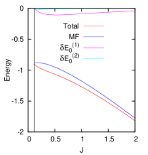
Figure 3: Contributions to the ground state energy per site: mean-field energy and Møller-Plesset correction. The vertical line denotes $J_{min}/t$ where $s\rightarrow 0$.

The unperturbed energy of this state is $E_{\beta,{\bm{q}}}+\tilde{J}-E_{\alpha,{\bm{p}}}+E_{0}$, because the triplet which is created along with the particle-hole pair contributes the energy $\tilde{J}$ if we neglect the dispersion of the triplets. The matrix element for the transition can be evaluated by using (14) and is

$$\frac{s}{2N}\;e^{i({\bm{p}}-{\bm{q}})\cdot{\bm{R}}_{n}}\;m_{{\bm{p}},{\bm{q}}}$$

with

$$m_{{\bm{p}},{\bm{q}}} = \epsilon_{\bm{q}}u_{\bm{p}}(u_{\bm{q}}+v_{\bm{q}})-\epsilon_{\bm{p}}u_{\bm{q}}(u_{\bm{p}}-v_{\bm{p}}).$$

The correction to the energy/site due to creation of a single triplet then is

$$\delta E_{0}^{(1)} = -\frac{3s^{2}}{2N^{2}}\;\sum_{{\bm{p}},{\bm{q}}}\;\frac{m_{{\bm{p}},{\bm{q}}}^{2}}{E_{\beta,{\bm{q}}}+\tilde{J}-E_{\alpha,{\bm{p}}}}.$$ (15)

We proceed to the correction due to $H_{2}$ and $H_{4}$. The parts which give a nonvanishing result when acting onto the vacuum for triplets are

$$H_{2}^{\prime} = \;\sum_{m,n}\;\frac{t_{m,n}}{2}\left(\;a_{n,\downarrow}b_{m,\uparrow}-a_{n,\uparrow}b_{m,\downarrow}\;\right)\;{\bm{t}}^{\dagger}_{m}\cdot{\bm{t}}^{\dagger}_{n}$$

$$H_{4}^{\prime} = -i\;\sum_{m<n}\;\frac{t_{m,n}}{2}\left(\;{\bm{\pi}}_{m,n}-{\bm{\pi}}_{n,m}\;\right)\cdot({\bm{t}}^{\dagger}_{m}\times{\bm{t}}^{\dagger}_{n})$$

The states which can be reached have the form $\beta_{{\bm{q}},\sigma}^{\dagger}\alpha_{{\bm{p}},\sigma^{\prime}}{\bm{t}}_{n,x}^{\dagger}{\bm{t}}_{m,x^{\prime}}^{\dagger}|GS\rangle$. Proceeding as above and specializing to a 1D chain with only nearest neighbor hopping $-t$ we find for the energy shift due to the creation of two triplets

$$\delta E_{0}^{(2)} = -\frac{9t^{2}}{N^{2}}\;\sum_{{\bm{p}},{\bm{q}}}\;\frac{(1+\cos({\bm{p}}+{\bm{q}}))\;u_{\bm{p}}^{2}u_{\bm{q}}^{2}}{E_{\beta,{\bm{q}}}+2\tilde{J}-E_{\alpha,{\bm{p}}}}.$$ (16)

The different contributions to the ground state energy are shown in Figure 3. The perturbation correction is quite small which indicates that the use of perturbation theory is adequate. The energy shift due to creation of a single triplet, $\delta E_{0}^{(2)}$ is small but still of order $0.1t$, whereas $\delta E_{0}^{(3)}$ is negligible, of order $10^{-2}t$.

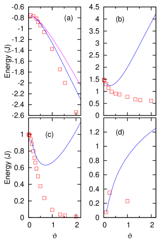
Figure 4: Characteristic energies for the 1D Kondo-insulator by bond-particle mean-field theory (blue lines) compared to DMRGyuwhite (red squares): ground state energy/site (a), quasiparticle gap $\Delta_{QP}$ (b), spin gap $\Delta_{S}$ (c) and spin excitation bandwidth $W_{s}$ (d) versus $J/t$. The magenta line in (a) is the mean-field energy without Møller-Plesset correction, $\vartheta=t/J$

Lastly, we discuss an improved calculation of the triplet dispersion $\omega_{\bf k}$. While the mean-field calculation predicts these to be almost dispersionless the term $H_{3}$ gives a more substantial dispersion. We make the variational ansatz for a $z$-triplet-like excitation with momentum ${\bf q}$

$$|\Psi_{\bf q}\rangle = \left[\;a_{\bf q}{\bf t}_{{\bf q}}^{\dagger}+\frac{1}{\sqrt{2N}}\sum_{{\bm{k}},\sigma,\sigma^{\prime}}b_{{\bf q},{\bf k}}\;\beta_{{\bf k}+{\bf q},\sigma}^{\dagger}{\bm{\tau}}_{\sigma,\sigma^{\prime}}\alpha_{{\bf k},\sigma^{\prime}}\;\right]|0\rangle,$$

with variational parameters $a_{\bf q}$ and $b_{{\bf q},{\bf k}}$. We obtain the triplet frequency

$$\tilde{\omega}_{\bm{q}} = \tilde{J}+\frac{s^{2}}{2N}\;\sum_{\bm{k}}\;\frac{V^{2}({\bm{k}},\bm{q})}{\tilde{\omega}_{\bm{q}}-(E_{\beta,{\bm{k}}+\bm{q}}-E_{\alpha,{\bm{k}}})}$$

$$V({\bm{k}},\bm{q}) = (\epsilon_{{\bm{k}}+\bm{q}}-\epsilon_{{\bm{k}}})\;v_{{\bm{k}}+\bm{q}}v_{{\bm{k}}}$$ (18)

$$\;\;\;\;\;\;\;\;+\epsilon_{{\bm{k}}+\bm{q}}\;u_{{\bm{k}}+\bm{q}}v_{{\bm{k}}}+\epsilon_{{\bm{k}}}\;u_{{\bm{k}}}v_{{\bm{k}}+\bm{q}},$$

where $\epsilon_{{\bm{k}}}$ is the noninteracting dispersion of the conduction electrons. Numerical evaluation shows that this always takes its minimum at $k=\pi$ and the maximum at $k=0$ - consistent with DMRGyuwhite . The energy $\tilde{\omega}_{q=\pi}$ thus is the energy of the lowest $S=1$ excitation, called the spin gap, $\Delta_{s}$. The bandwidth of the spin excitations is $W_{s}=\tilde{\omega}_{q=0}-\tilde{\omega}_{q=\pi}$. Figure 4 compares the dependence of the ground state energy per site, the quasiparticle and spin gap and the bandwidth of the spin excitations on $t/J$ for the 1D Kondo insulator to results obtained by DMRGyuwhite . As expected, the perturbation correction improves the ground state energy/site, which is reasonably close to the numerical values for $t/J<1$. For all other quantities the calculated energies deviate from the numerical results already for relatively large $J/t$. One might wonder if this is the consequence of the additional approximation to neglect $\tilde{\eta}$, but even for $J/t=1$ where the boson bandwidth is quite small (see Figure 2) the deviation for the spin gap is already substantial. To conclude this section we discuss the differences to the previous mean-field treatment in Ref.JureckaBrenig . In this work, both the singlet and the triplet operators in (10) were replaced by $c$-numbers, $s_{n}^{\dagger},s_{n}\rightarrow s$ and $\bm{t}_{n}^{\dagger},\bm{t}_{n}\rightarrow\bm{t}\;e^{i\bm{Q}\cdot\bm{R}_{n}}$, thus reducing (10) to a quadratic form from the outset, and then minimizing $F$ with respect to $s$ and $\bm{t}$. The dynamics of the spin excitations thereby was not studied.

IV Renormalized Energy of Formation

We consider a different approximation scheme to account for the constraint whereby we consider sites occupied by a singlet as ‘empty’. This is equivalent to working in a fictitious Hilbert space for the fermionic particles $a^{\dagger}_{n,\sigma}$ and $b^{\dagger}_{n,\sigma}$ as well as the triplets ${\bf t}^{\dagger}_{n,\alpha}$, whereby the states in this fictitious Hilbert space correspond to those of the physical Kondo lattice according to the rule

$$\prod_{i\in S_{a}}a_{i,\sigma_{i}}^{\dagger}\;\prod_{j\in S_{b}}b_{j,\sigma_{j}}^{\dagger}\;\prod_{l\in S_{t}}t_{l,x_{l}}^{\dagger}|0\rangle\rightarrow\;\;\;\;\;\;\;\;\;\;\;\;\;\;\;\;\;\;\;\;\;\;\;\;\;\;\;$$

$$\bigotimes_{i\in S_{a}}|a,i,\sigma_{i}\rangle\;\bigotimes_{j\in S_{b}}|b,j,\sigma_{j}\rangle\;\bigotimes_{l\in S_{t}}|t_{x_{l},l}\rangle\;\bigotimes_{n\in S_{s}}\;|s_{n}\rangle.$$ (19)

$S_{a}$, $S_{b}$ and $S_{t}$ denote the set of sites occupied by a hole-like fermion, an electron-like fermion or a triplet, respectively, and $S_{s}=(S_{a}\cup S_{b}\cup S_{t})^{C}$ the set of remaining sites. In other words, all sites not occupied by a fermion or triplet are filled up with ‘inert’ singlets. The Hamiltonian - and all other operators in the bond particle representation - then can be obtained from (10) by replacing all singlet operators by unity. Only the form (6) of the exchange term can be used. For this representation to make sense we again have to impose the constraint that no two particles of any type occupy the same site, because the resulting state could not be translated meaningfully to a state of the physical Kondo lattice via (19). Assuming that the density of bond particles is small, however, we relax again this constraint.
On the other hand, if the constraint were rigorously enforced, presence of any one particle - be it $a^{\dagger}_{n,\sigma}$, $b^{\dagger}_{n,\sigma}$ or ${\bf t}^{\dagger}_{n,\alpha}$ - at a given site $n$ would prevent all remaining terms in the Hamiltonian which involve creation or annihilation of any other particle at site $n$ from acting, resulting in a loss of kinetic energy. The constraint thus increases the cost in energy for adding a fermion or boson. Accordingly, in (6) the energy for adding a fermion therefore should be $e_{0}=3J/4+\kappa$ rather than $3J/4$ and the energy for adding a boson $\tilde{J}=J+\kappa$ rather than $J$, where $\kappa$ is some as yet unspecified loss of kinetic energy. Actually $\kappa$ may be expected to be different for fermions and bosons. We will discuss possible estimates for $\kappa$ later on. It should also be noted that such an increase of the energies of formation of the particles would reduce their densities and thus make relaxing the constraint of no double occupancy an even better approximation. The mean-field theory outlined in the previous section and the approximation scheme discussed in the present section mimick the constraint in different ways: mean-field theory amounts to a Gutzwiller-like downward renormalization of the hopping integrals whereas the present scheme amounts to a higher energy of formation of the particles. Collecting all terms which become quadratic when we drop the singlets we obtain the noninteracting Hamiltonian

$$H_{0} = \sum_{n}\;\left(\;e_{0}\;\sum_{\sigma}\;(b_{n,\sigma}^{\dagger}b_{n,\sigma}+a_{n,\sigma}^{\dagger}a_{n,\sigma})+\tilde{J}\;\bm{t}_{n}^{\dagger}\cdot\bm{t}_{n}\;\right)+\sum_{m,n}\;\frac{t_{m,n}}{2}\;\sum_{\sigma}\;\left(\;b_{m,\sigma}^{\dagger}b_{n,\sigma}-a_{m,\sigma}^{\dagger}a_{n,\sigma}\;\right)$$

$$\;\;\;\;-\sum_{m,n}\;\frac{t_{m,n}}{2}\;\left[\;\left(\;b_{m,\uparrow}^{\dagger}a_{n,\downarrow}^{\dagger}-b_{m,\downarrow}^{\dagger}a_{n,\uparrow}^{\dagger}\;\right)+H.c.\;\right]-\frac{3NJ}{4}.$$

The interaction part of the Hamiltonian is the sum of

$$H_{2} = \sum_{m,n}\;\frac{t_{m,n}}{2}\;\sum_{\sigma}\;\left(\;b_{m,\sigma}^{\dagger}b_{n,\sigma}-a_{m,\sigma}^{\dagger}a_{n,\sigma}\;\right)\;\bm{t}_{n}^{\dagger}\cdot\bm{t}_{m}\;+\sum_{m,n}\;\frac{t_{m,n}}{2}\;\left[\;\left(\;b_{m,\uparrow}^{\dagger}a_{n,\downarrow}^{\dagger}-b_{m,\downarrow}^{\dagger}a_{n,\uparrow}^{\dagger}\;\right)\bm{t}_{m}\cdot\bm{t}_{n}\;+H.c\;\right]$$

$$H_{3} = -\;\sum_{m,n}\;\frac{t_{m,n}}{2}\;\left[\;\left(\;{\bm{\pi}}^{\dagger}_{m,n}\cdot\left(\;\bm{t}_{n}-\bm{t}_{m}\right)+H.c.\;\right)+\left(\;\bm{b}_{m,n}-\bm{a}_{m,n}\;\right)\cdot(\bm{t}_{n}^{\dagger}+\bm{t}_{m}\;)\;\right],$$

$$H_{4} = \sum_{m,n}\;\frac{t_{m,n}}{2}\;\left[\;\left[\;i{\bm{\pi}}^{\dagger}_{m,n}\cdot(\;\bm{t}_{m}\times\bm{t}_{n}\;)+H.c.\;\right]-i\;(\;\bm{b}_{m,n}-\bm{a}_{m,n}\;)\;(\;\bm{t}_{n}^{\dagger}\times\bm{t}_{m}\;)\;\right].$$ (20)

The part $H_{0}$ was used in Refs.Oana ; afbf . Due to particle-hole symmetry the extra Lagrange multiplier introduced in these Refs. to enforce consistency of the $c$-like spectral weight with $N_{e}$ is not necessary here. We now proceed as in the case of mean-field theory, that means first diagonalize $H_{0}$ to obtain the band structure and treat the interaction terms in the same approximation as there, i.e. in perturbation theory for the ground state energy and using the variational ansatz (LABEL:svar) for the spin excitations. The fermionic part $H_{F}$ again can be diagonalized by the unitary transformation (14) with the result

$$H_{F} = \sum_{\bm{k},\sigma}\;(\;E_{\alpha,\bm{k}}\;\alpha_{\bm{k},\sigma}^{\dagger}\alpha_{\bm{k},\sigma}+E_{\beta,\bm{k}}\;\beta_{\bm{k},\sigma}^{\dagger}\beta_{\bm{k},\sigma}\;)$$

$$\;\;\;\;\;\;\;\;\;\;\;\;\;\;\;\;\;\;\;\;\;\;\;\;\;\;\;\;\;\;\;\;-\;2\sum_{\bm{k}}\;(\frac{\epsilon_{\bm{k}}}{2}-e_{0}),$$

$$E_{\nu,\bm{k}} = \frac{\epsilon_{\bm{k}}}{2}\pm W_{\bm{k}}-\mu,$$

$$W_{\bm{k}} = \sqrt{e_{0}^{2}+\left(\frac{\epsilon_{\bm{k}}}{2}\right)^{2}},$$

$$u_{\bm{k}} = -\sqrt{\frac{W_{\bm{k}}-e_{0}}{2W_{\bm{k}}}},$$

$$v_{\bm{k}} = \frac{-\frac{\epsilon_{\bm{k}}}{2}}{\sqrt{2W_{\bm{k}}(W_{\bm{k}}-e_{0})}}.$$

The noninteracting ground state for the bosons is the bosonic vacuum i.e. the bosons do not contribute to the ground state energy $E_{0}$ in this approximation. The Helmholtz Free energy is

$$F = -\frac{2}{\beta}\;\sum_{\bm{k}}\;\sum_{\nu\in\{\alpha,\beta\}}\;\log\left(1+e^{-\beta E_{\nu,\bm{k}}}\right)$$

$$\;\;\;\;\;\;\;\;+N(2e_{0}-\frac{3J}{4})+\mu N.$$

We can obtain the expectation value of the kinetic energy by multiplying all hopping integrals by a parameter $\chi$: $t_{m,n}\rightarrow\chi t_{m,n}$ and forming $\frac{\partial F}{\partial\chi}|_{\chi=1}$, with the result:

$$k = \frac{1}{N}\;\sum_{{\bm{k}}}\;\left[\;\epsilon_{{\bm{k}}}\left(\;1-\frac{\epsilon_{{\bm{k}}}}{2W_{{\bm{k}}}}\;\right)f(E_{\alpha,{\bm{k}}})\right.$$ (21)

$$\left.\;\;\;\;\;\;\;\;\;\;\;\;\;\;\;\;+\epsilon_{{\bm{k}}}\left(\;1+\frac{\epsilon_{{\bm{k}}}}{2W_{{\bm{k}}}}\;\right)f(E_{\beta,{\bm{k}}})\right].$$

Treating the interaction part $H_{2}+H_{3}+H_{4}$ in 2^nd order perturbation theory a slight modification occurs. Since the ground state is the vacuum for bosons and the vector operators ${\bf a}$, ${\bf b}$ and ${\bf\pi}$ have zero expectation value in the fermionic ground state (which is spin singlet) only intermediate states which contain both, a bosonic and a fermionic excitation, can be reached from the ground state by acting with $H_{3}$ or $H_{4}$. The energy shifts due to such doubly excited intermediate states take the form (15), (16), but with $s\rightarrow 1$ in (15). In addition, however, the term $H_{2}$ also has a nonvanishing matrix element with states of the form ${\bf t}_{m}^{\dagger}\cdot{\bf t}_{n}^{\dagger}|GS\rangle$, because the fermionic factor of the corresponding term is a singlet, which does have a nonvanishing ground state expectation value. For the 1D chain with nearest neighbor hopping this gives an additional contribution to $\delta E_{0}^{(2)}$ of $-3\;\frac{I^{2}}{2\tilde{J}}$, whereby

$$I = -\frac{t^{2}}{N}\;\sum_{q}\;\frac{\cos^{2}(q)}{W_{q}}.$$ (22)

Numerical evaluation shows that this contribution is quite substantial and obviously this replaces the energy gain due to the mean-field factorized terms in the previous section. Finally, the equation for the dispersion of the spin excitation takes the form (18), again with $s\rightarrow 1$.

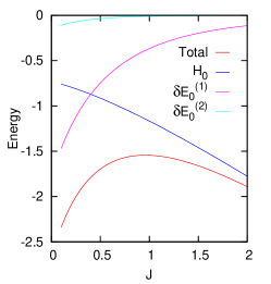
Figure 5: Contributions to the ground state energy per site: Contribution from $H_{0}$ and corrections from perturbation theory.

Lastly, we consider the value of $\kappa$, the correction to the energies of formation of the fermions and bosons.

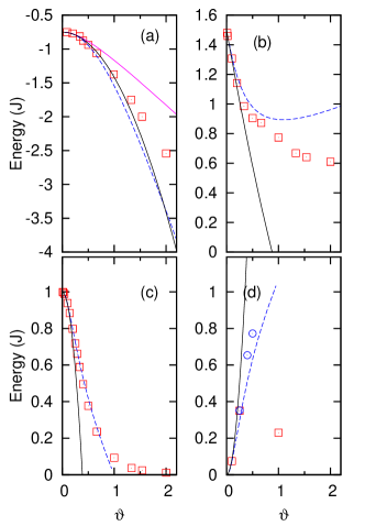
Figure 6: Characteristic energies in the 1D Kondo-insulator from the renormalized energy of formation scheme with $x=0.4$ (blue lines) compared to DMRGyuwhite (red squares) and SEseriesexp (blue circles): ground state energy/site (a), quasiparticle gap $\Delta_{QP}$ (b), spin gap $\Delta_{S}$ (c) and spin excitation bandwidth $W_{s}$ (d) versus $J/t$. The magenta line in (a) is the energy from $H_{0}$ without perturbation theory correction. The black lines are obtained by perturbation expansion in $t/J$uedareview , $\vartheta=t/J$.

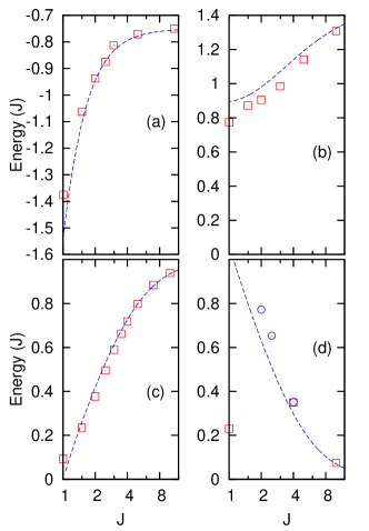
Figure 7: Same as Figure 6 but all energies plotted versus $J/t$ in the range $J/t\geq 1$.

We switch to a phenomenological approach and approximate $\kappa\approx xk$, i.e. a dimensionless parameter $x$ times the kinetic energies of the Fermions/site, given in (21). With $x$ fixed, $\kappa$ has to be determined self-consistently for each $J/t$. We neglect the loss of kinetic energy of bosons which is reasonable for $J/t>1$ where the boson density is low. In fact, as will be shown in a moment, we can obtain good agreement with numerics over the whole range $J/t>1$ by choosing $x\approx 0.4$ independent of $JJ/t$. Varying $0.2<x<0.6$ thereby does not deteriorate the agreement significantly, so that also an $x$ which varies with $J/t$ - which is actually what one might expect - would give similar results.
To begin with, Figure 5 shows the various contributions to the ground state energy/site obtained with this choice of $x$ and demonstrates that at least for $J/t>1$ the perturbation correction is small as it should be. Figure 6 compares characteristic energies of the system as functions of $t/J$ to numerical results. For larger $t/J>1$ the agreement is poor, in particular for $t/J\approx 1$ the spin excitation energy $\tilde{\omega}_{q}$ from the variational ansatz becomes negative around $q=\pi$ indicating the failure of the calculation. Accordingly, results for the spin gap $\Delta_{s}$ and spin excitation bandwidth $W_{s}$ are shown only up to this value of $t/J$. $W_{s}$ comes out quite good for $t/J<1$ - the Figure also shows the very good agreement between DMRG and SE for $W_{s}$ at $t/J=0.25$ in (d). DMRG and SE also agree very well for $\Delta_{s}$ so that we do not show the SE results in (c). Figure 6 also shows results obtained by perturbation expansion in $t/J$uedareview . As one might have expected the DMRG results and bond particle theory approach these for $t/J\rightarrow 0$. The ground state energy is reproduced remarkably well be the perturbation expansion, but all other characteristic energies deviate substantially from the perturbation expansion for $t/J\rightarrow 1$. This shows that despite being a strong coupling theory by nature, bond particle theory does go beyond simple perturbation theory. Figure 7 shows the same characteristic energies but now plotted versus $J/t$ in the range $J/t>1$. It is obvious that in this range the agreement between bond particle theory and numerics is quite good. Figure 8 shows the densities of fermions and bosons, $n_{F}$ and $n_{B}$. Thereby $n_{B}$ is obtained from $n_{B}=\frac{\partial E_{0}}{\partial\tilde{J}}$ where $E_{0}$ is the ground state energy per site including the second order perturbation correction. The main contribution thereby comes from (22). The data points for $t/J=1$ are DMRG resultsyuwhite . The densities are small for $t/J<1$ and bond particle theory somewhat underestimates the densities of the particles at $t/J=1$. For larger $t/J$ the densities increase rapidly and the sum $n_{B}+n_{F}$ exceeds $1$ at $t/J\approx 2$, indicating the breakdown of bond particle theory. Figure 9 shows the band structure of the fermions and the dispersion of the bosons obtained from the variational ansatz. For $J/t=2$ the dispersions can be compared to results obtained by SE taken from Ref. seriesexp . While the quasiparticle gap is approximately correct, the ‘heavy’ part of the band structure has too much dispersion as compared to SE, and the bandwidth is slightly overestimated. The dispersion of the spin excitations is reasonably correct for $J/t=2$, both the spingap, the overall form of the dispersion and the bandwidth compare quite well with the SE result.

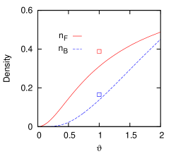
Figure 8: Densities of fermions and bosons for the 1D Kondo insulator versus $\theta=t/J$, data points from DMRGyuwhite .

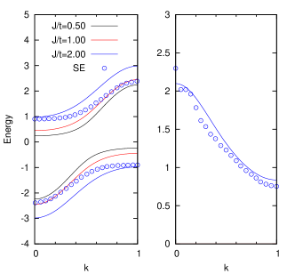
Figure 9: Band structure of the fermions (left) and boson dispersion from the variational ansatz (18) (right) for different $J/t$, wave vectors in units of $\pi$. Data points obtained by SE for $J/t=2$seriesexp . The boson dispersion for $J/t=1$ and $J/t=0.5$ is not given because there the variational calculation gives negative energy over some range of $k$.

The combined DMRG and SE data in Figure 6 suggest that there is a crossover between two regimes at around $t/J\approx 1$: the $\Delta_{s}/J$ vs. $J/t$ curve drops rapidly for $J/t>1$ but then bends sharply at $J/t\approx 1$ and $\Delta_{s}/J$ is small but finite for $J/t<1$. Similarly, the band width of the spin excitations, $W_{s}/J$ increases with decreasing $J/t$ in the range $J/t>1$ but then must drop sharply at $J/t\approx 1$. This may indicate a crossover from a strong coupling regime for $J/t>1$ where the system apparently can be described well by the bond particle theory, to a weak coupling regime for $J/t<1$ where maybe mean-field theories work better. It should also be noted that the present theory must fail in the limit $J/t\rightarrow 0$ not only because the bond particle density increases sharply but also because for because $J/t\rightarrow 0$ the quasiparticle gap vanishes, whereas the energy $e_{0}$ - which determines the magnitude of the gap - cannot approach zero for any $x>0$. All in all Figure 6 indicates that for $t/J<1$ the bond-particle Hamiltonian (20) with suitably renormalized energies of formation gives a reasonably correct description of the low-energy elementary excitations of the 1D Kondo insulator.

V Summary and Discussion

In summary we have derived an exact representation of the Kondo lattice model in terms of bond particles: fermions corresponding to unit cells with an odd number of electrons and bosons corresponding to cells with two electrons coupled to a singlet or triplet. Thereby the constraint to have precisely one $f$ electron/cell, which considerably complicates the solution of the KLM, is fulfilled automatically and replaced by the constraint to have precisely one bond particle per site. If the singlet bosons are considered as condensed or the singlet is defined as the vaccum state of a cell, this constraint becomes an infinitely strong Hubbard-like repulsion, but for a relatively dilute system of particles, so that it may be justified to relax it (for a system of low density even an infinitely strong repulsion can be treated diagrammaticallyFW ; Kotov ; Shevchenko ). The requirement of low particle density is indeed fulfilled for $J/t>1$.
We have discussed two schemes to approximately incorporate effects of the remaining Hubbard repulsion between bond particles into their Hamiltonian. First, mean-field theory, where the singlets are taken as condensed, amounts to a Gutzwiller-like downward renormalization of all hopping integrals. Second, a scheme where the singlet is considered as the vacuum state of a site and the constraint is mimicked by adding the loss of kinetic energy, which incurs due to the blocking of a site by a bond particle, to the energy ascribed to the respective particle. Approximating this loss of kinetic energy as the kinetic energy of fermions per site times a phenomenological constant of order unity allowed to reproduce numerical results ontained by density matrix renormalization group and series expansion calculations for the 1D Kondo insulator in the range $J/t>1$ with good accuray. Thereby relatively simple techniques were used - 2^nd order perturbation theory for the ground state energy and the simplest possible variational wave function for the triplet dispersion - to produce these results. The good agrement with numerics in the range $J/t>1$ for a variety of quantitiesis then is a strong indication that in this parameter range the triplets and fermions indeed correspond to the approximate elementary excitations and this is the main result of the present paper. Despite being a somewhat lengthy expression the bond particle Hamiltonian with renormalized particle energies appears to be useful for quantitative calculations. Of course the phenomenological approach used here is somewhat unsatisfactory and a more rigorous calculation following Refs. Kotov ; Shevchenko would be desirable.
The question then arises, whether $J/t>1$ is a sufficient range of validity to discuss magnetic ordering and quantum critical points in the KLM. For the 2D square lattice with nearest neighbor hopping it is known that at $n_{e}=2$ and $T=0$ antiferromagnetic ordering occurs for $J/t\leq J_{c}/t=1.45$Assaad , i.e. for relatively large $J/t$ (although with the information at hand we cannot say much about the range of vailidity of the bond particle description in higher dimensions). As pointed out by Sachdev and BhattSachdevBhatt bond particle theory gives a rather natural description of magnetic ordering, namely the condensation of triplets into a momentum corresponding to the magnetic ordering wave vector. Applying this description of antiferromagnetic ordering in the KLM has already produced encouraging results: using the mean-field version of bond particle theory with condensed triplets, Jurecka and Brenig found $J_{c}/t=1.5$, quite close to the exact value. This is even more remarkable in that even numerical methods appear to have difficulties to accurately reproduce $J_{c}/t$: VMC gives $J_{c,1}/t=1.7$WatanabeOgata , DCA gives $J_{c,1}/t=2.1$MartinBerxAssaad , and DMFT gives $J_{c,1}/t=2.2$K13 . Moreover, in Ref. afbf it was shown that using unrenormalized energies of formation (i.e. $\kappa=0$) bond particle theory for the planar KLM did give the too large $J_{c}/t=2.20$ but reproduced the phase diagram of the model in the $(J/t,n_{e})$-plane obtained by VMCWatanabeOgata and DMFTK13 quite well if $J$ was measured in units of $J_{c}$ - i.e. if the phase diagram was plotted in the $(J/J_{c},n_{e})$ plane - so that the error in $J_{c}/t$ cancelled to some degree. This is encouraging in that the phase diagram of the KLM in 2D is quite intricate, comprising the paramagnetic and two antiferromagnetic phases with different Fermi surface topology, with various 1^st and 2^nd order transitions between them. Also, the band structure in the AF phase and its change with $J/J_{c}$ as obtained by DCAMartinBerxAssaad could be reproduced in this wayafbf1 . It should also be noted that in the above bond particle calculations antiferromagnetic order appears without an additional Heisenberg exchange between $f$ spins, that means it comes about solely by the interaction mediated by the conduction electrons.

References

- (1) G. R. Stewart, Rev. Mod. Phys. 56, 755 (1984).
- (2) P. A. Lee, T. M. Rice, J. W. Serene, L. J. Sham, and J. W. Wilkins, Comm. in Condensed Matter Phys. 12, 99 (1986).
- (3) G. R. Stewart,Rev. Mod. Phys. 73, 797 (2001).
- (4) H. v. Löhneysen, A. Rosch, M. Vojta, and P. Wölfle, Rev. Mod. Phys. 79, 1015 (2007).
- (5) Q. Si and F. Steglich, Science 329, 1161 (2010).
- (6) J. R. Schrieffer and P. A. Wolff, Phys. Rev. 149, 491 (1966).
- (7) K. Yosida, Phys. Rev. 147, 223 (1966).
- (8) C. M. Varma and Y. Yafet, Phys. Rev. B 13, 2950 (1976).
- (9) O. Gunnarsson and K. Schönhammer, Phys. Rev. B 28, 4315 (1983).
- (10) A. Yoshimori and A. Sakurai, Progr. Theor. Phys. Supp. 46, 162 (1970).
- (11) N. Read and D. M. Newns, J. Phys. C 16, 3273 (1983).
- (12) H. Keiter and J. C. Kimball, Int. J. Magn. 1, 233 (1971).
- (13) Y. Kuramoto, Z. Phys. B 53, 37 (1983).
- (14) P. Coleman, Phys. Rev. B 29, 3035 (1984).
- (15) N. E. Bickers, Rev. Mod. Phys. 59, 845 (1987).
- (16) K. G. Wilson, Rev. Mod. Phys. 47, 773 (1975).
- (17) N. Andrei, K. Furaya, and J. H. Lowenstein, Rev. Mod. Phys. 55, 331 (1983).
- (18) M. Oshikawa, Phys. Rev. Lett. 84, 3370 (2000).
- (19) C. Lacroix and M. Cyrot, Phys. Rev. B 20, 1969 (1979).
- (20) C. Lacroix, Solid State Commun. 54, 991 (1985).
- (21) A. Auerbach and K. Levin, Phys. Rev. Lett. 57, 877 (1986).
- (22) S. Burdin, A. Georges, and D. R. Grempel, Phys. Rev. Lett. 85, 1048 (2000).
- (23) G.-M. Zhang and L. Yu, Phys. Rev. B 62, 76 (2000).
- (24) M. Lavagna and C. Pepin, Phys. Rev. B 62, 6450 (2000).
- (25) T. Senthil, M. Vojta, and S. Sachdev, Phys. Rev. B 69, 035111 (2004).
- (26) M. Vojta, Phys. Rev. B 78, 125109 (2008).
- (27) G.-M. Zhang, Y.-H. Su, and L. Yu, Phys. Rev. B 83, 033102 (2011).
- (28) J. Nilsson, Phys. Rev. B 83, 235103 (2011).
- (29) X. Montiel, S. Burdin, C. Pepin, and A. Ferraz, Phys. Rev. B 90, 045125 (2014).
- (30) A. J. Millis and P. A. Lee, Phys. Rev. B 35, 3394 (1987).
- (31) D. M. Newns and N. Read, Adv. Phys. 36, 799 (1987).
- (32) T. M. Rice and K. Ueda, Phys. Rev. Lett. 55, 995 (1985).
- (33) P. Fazekas and E. Müller-Hartmann, Z. Phys. B 85, 285 (1991).
- (34) C. C. Yu and S. R. White, Phys. Rev. Lett. 71, 3866 (1993). The DMRG data for the ground state energy are not published in this reference but seem to be given only in Ref. series .
- (35) S. Moukouri and L. G. Caron, Phys. Rev. B. 52,15723(R) (1995).
- (36) S. Moukouri and L. G. Caron, Phys. Rev. B. 54,12212 (1996).
- (37) T. Mutou, N. Shibata, and K. Ueda, Phys. Rev. Lett. 81, 4939 (1998).
- (38) S. Smerat, U. Schollwöck, I. P. McCulloch, and H. Schoeller Phys. Rev. B 79, 235107 (2009).
- (39) M. Jarrell, H. Akhlaghpour, and Th. Pruschke Phys. Rev. Lett. 70, 1670 (1993).
- (40) M. Jarrell, Phys. Rev. B 51, 7429 (1995).
- (41) A. N. Tahvildar-Zadeh, M. Jarrell, and J. K. Freericks, Phys. Rev. Lett. 80, 5168 (1998).
- (42) R. Peters and T. Pruschke Phys. Rev. B 76, 245101 (2007).
- (43) C. Gröber and R. Eder, Phys. Rev. B. 57,12659(R) (1998).
- (44) F. F. Assaad, Phys. Rev. Lett. 83, 796 (1999).
- (45) Z.-P. Shi, R. R. P. Singh, M. P. Gelfand, and Z. Wang Phys. Rev. B 51, 15630(R) (1995).
- (46) W. Zheng and J. Oitmaa, Phys. Rev. B 67, 214406 (2003).
- (47) S. Trebst, H. Monien, A. Grzesik, and M. Sigrist, Phys. Rev. B 73, 165101 (2006).
- (48) H. Watanabe and M. Ogata, Phys. Rev. Lett. 99, 136401 (2007).
- (49) M. Z. Asadzadeh, F. Becca, and M. Fabrizio, Phys. Rev. B 87, 205144 (2013).
- (50) K. Kubo, J. Phys. Soc. Jpn. 84, 094702 (2015).
- (51) H. Tsunetsugu, Y. Hatsugai, K. Ueda, and M. Sigrist, Phys. Rev. B 46, 3175 (1992).
- (52) J. A. White, Phys. Rev. B 46, 13905 (1992).
- (53) K. Tsutsui, Y. Ohta, R. Eder, S. Maekawa, E. Dagotto, and J. Riera, Phys. Rev. Lett. 76, 279 (1996).
- (54) L. C. Martin and F. F. Assaad, Phys. Rev. Lett. 101, 066404 (2008).
- (55) L. C. Martin, M. Bercx, and F. F. Assaad, Phys. Rev. B 82, 245105 (2010).
- (56) B. Lenz, R. Gezzi, and S. R. Manmana, Phys. Rev. B 96, 155119 (2017).
- (57) S. Doniach, Physica B 91, 231 (1977).
- (58) M. A. Ruderman and C. Kittel Phys. Rev. 96, 99 (1954); T. Kasuya, Progress of Theoretical Physics, 16, 45 (1956); K. Yosida, Phys. Rev. 106, 893 (1957).
- (59) Q. Si, S. Rabello, K. Ingersent, and J. Smith, Nature 413, 804 (2001).
- (60) Q. Si, S. Rabello, K. Ingersent, and J. L. Smith, Phys. Rev. B 68, 115103 (2003).
- (61) L. De Leo, M. Civelli, and G. Kotliar, Phys. Rev. Lett. 101, 256404 (2008).
- (62) L. Zhu and Q. Si, Phys. Rev. B 66, 024426 (2002).
- (63) J. X. Zhu, D. R. Grempel, and Q. Si, Phys. Rev. Lett. 91, 156404 (2003).
- (64) P. Sun and G. Kotliar, Phys. Rev. Lett. 91, 037209 (2003).
- (65) S. J. Yamamoto and Q. Si, Phys. Rev. Lett. 99, 016401 (2007).
- (66) M. T. Glossop and K. Ingersent, Phys. Rev. Lett. 99, 227203 (2007).
- (67) J.-X. Zhu, S. Kirchner, R. Bulla, and Q. Si, Phys. Rev. Lett. 99, 227204 (2007).
- (68) Q. Si, J. H. Pixley, E. Nica, S. J. Yamamoto, P. Goswami, R. Yu, and S. Kirchner, J. Phys. Soc. Jpn. 83, 061005 (2014).
- (69) E. Abrahams, J. Schmalian, and P. Wölfle, Phys. Rev. B 90, 045105 (2014).
- (70) R. Peters and N. Kawakami, Phys. Rev. B 92, 075103 (2015).
- (71) R. Peters and N. Kawakami, Phys. Rev. B 96, 115158 (2017).
- (72) S. Sachdev and R. N. Bhatt, Phys. Rev. B 41, 9323 (1990).
- (73) S. Gopalan, T. M. Rice, and M. Sigrist, Phys. Rev. B 49, 8901 (1994).
- (74) M. Vojta and K. W. Becker, Phys. Rev. B 60, 15201 (1999).
- (75) S. Ray and M. Vojta, Phys. Rev. B 98, 115102 (2018).
- (76) O. P. Sushkov, Phys. Rev. B 60, 3289 (1999).
- (77) K. Park and S. Sachdev, Phys. Rev. B 64, 184510 (2001).
- (78) M. Siahatgar, B. Schmidt, G. Zwicknagl, and P. Thalmeier, New J. Phys. 14, 103005 (2014).
- (79) R. Eder, O. Stoica, and G. A. Sawatzky, Phys. Rev. B. 55, R6109 (1997); R. Eder, O. Rogojanu, and G. A. Sawatzky, Phys. Rev. B. 58, 7599 (1998).
- (80) C. Jurecka and W. Brenig, Phys. Rev. B 64, 092406 (2001).
- (81) V. N. Kotov and P. Hirschfeld, Physica B: Condensed Matter, 312-313, 174 (2002).
- (82) R. Eder, K. Grube, and P. Wróbel, Phys. Rev. B 93, 165111 (2016).
- (83) R. Eder and P. Wróbel, Phys. Rev. B 98, 245125 (2018).
- (84) P. Nozieres, Eur. Phys. J. B 6, 447 (1998).
- (85) See, e.g., A. L. Fetter and J. D. Walecka, Quantum Theory of Many Particle Systems (McGraw-Hill, New York, 1971).
- (86) V. N. Kotov, O. Sushkov, ZhengWeihong, and J. Oitmaa, Phys. Rev. Lett. 80, 5790 (1998).
- (87) P. V. Shevchenko, A. W. Sandvik, and O. P. Sushkov Phys. Rev. B 61, 3475 (2000).
- (88) H. Tsunetsugu, M. Sigrist, and K. Ueda Rev. Mod. Phys. 69, 809 (1997).
- (89) D. D. Johnson, Phys. Rev. B. 38, 12807, (1988).
- (90) C. Møller and M. S. Plesset, Phys. Rev. 46 618 (1934).