11email: {leon.bungert,martin.burger,daniel.tenbrinck}@fau.de
Computing Nonlinear Eigenfunctions via Gradient Flow Extinction
Abstract
In this work we investigate the computation of nonlinear eigenfunctions via the extinction profiles of gradient flows. We analyze a scheme that recursively subtracts such eigenfunctions from given data and show that this procedure yields a decomposition of the data into eigenfunctions in some cases as the 1-dimensional total variation, for instance. We discuss results of numerical experiments in which we use extinction profiles and the gradient flow for the task of spectral graph clustering as used, e.g., in machine learning applications.
Keywords:
Nonlinear eigenfunctions Spectral decompositions Gradient flows Extinction profiles Graph clustering.1 Introduction
Linear eigenvalue problems are of utter importance and a classical tool in signal and image processing. A frequently used tool here is the Fourier transform which basically decomposes a given signal into eigenfunctions of the Laplacian operator and makes frequency-based filtering possible. In addition, such problems also find their applications in machine learning and the treatment of large data sets [16, 13]. However, for some applications – as for example certain graph clustering tasks – linear theory does not suffice to achieve satisfactory results. Therefore, nonlinear eigenproblems, which involve a nonlinear operator, have gained in popularity over the last years since they can be successfully applied in far more complex and interesting application scenarios. However, solving such nonlinear eigenproblems is a challenging task and the techniques heavily depend on the structure of the involved operator. The setting we adopt is the following: we consider a Hilbert space and study the eigenvalue problem related to the subdifferential of an absolutely one-homogeneous convex functional . A prototypical example for such a functional is the total variation. So called nonlinear eigenfunctions are characterized by the inclusion
| (1) |
where usually the normalization is demanded to have a interpretable eigenvalue . Note that the operator is nonlinear and multivalued, in particular eigenfunctions do not form linear subspaces. Important properties and characterizations of the nonlinear eigenfunctions are collected in [5]. Of particular interest in applications is the decomposition of some data into a linear combination of eigenfunctions which, for instance, allows for scale-based filtering in image processing [6, 10, 11] – analogously to linear Fourier methods. In other applications, as spectral graph clustering, one is rather interested in finding a specific eigenfunction that is in some way related to the data or captures topological properties of the domain. An important tool for this nonlinear spectral analysis is the so called gradient flow of the functional
| (GF) |
whose connection to which has been analysed in finite dimensions in [7] and in infinite dimensions in [5]. In particular, the authors proved that the gradient flow is able to achieve the above-mentioned decomposition task in some situations. Furthermore, it always generates one specific eigenfunction, called the extinction profile or asymptotic profile of (cf. [1] for the special case of total variation flow). This profile is given by the subsequential limit of as tends to the extinction time of the flow. A different flow which also generates an eigenfunction was introduced and analyzed in [2, 14]. A third way for obtaining eigenfunctions, being less rigorous and reliable, consists in computing the gradient flow (GF) of and checking for subgradients to be eigenfunctions.
The rest of this work is organized as follows: After recapping some notation and important results regarding gradient flows and associated eigenfunctions in Section 2, we analyze an iterative scheme in Section 3 which is based on extinction profiles and constitutes an alternative to the already existent decomposition into nonlinear eigenfunctions through subgradients of the gradient flow. Finally, in Section 4 we present some applications of extinction profiles, mainly to spectral clustering.
2 Gradient Flows and Eigenfunctions
Without loss of generality, we will assume that the data is orthogonal to the null-space of the functional which is denoted by . For the example of total variation, this corresponds to calculating with data functions of zero mean. Furthermore, we will only be confronted with eigenvectors of eigenvalue , which follows naturally from the gradient flow structure. Normalizing them to have unit norm, shows that a suitable eigenvalue for an element which meets is given by . A complete picture of the theory of gradient flows and nonlinear eigenproblems is given in [5], from where the following statements are taken.
An important property of the gradient flow (GF) is that it decomposes the data into subgradients of the functional , i.e., it holds
| (2) |
where the subgradients enjoy the regularity of being elements in and, furthermore, have minimal norm in the subdifferentials , i.e. for all . This naturally qualifies them for being eigenfunctions as it was shown in [5]. Furthermore, the solution of (GF) extincts to zero in finite time under generic conditions on the functional . More precisely, it has to satisfy a Poincaré-type inequality, namely that there is such that
| (3) |
holds for all which are orthogonal to the null-space of (cf. [5, Rem. 6.3]). Let us in the following assume that the solution of (GF) extincts at time , in other words for all . In that case, there is an increasing sequence of times converging to such that
| (4) |
is a non-trivial eigenfunction of , i.e., and . The element is referered to as an extinction profile of .
In the following, the term spectral case refers to the scenario that the subgradients in (GF) are eigenfunctions themselves, i.e., for all . Using this together with the fact that is decreasing in implies that (2) becomes a decomposition of the datum into eigenfunctions with decreasing eigenvalues. Several scenarios and geometric conditions for this to happen were investigated in [5]. For instance, if the functional is the total variation in one space dimension, a divergence and rotation sparsity term, or special finite dimensional -sparsity terms, one has this spectral case. Also for general , a special structure of the data (cf. [4, 5, 15]) can yield the spectral case. Let us conclude the nomenclature by introducing the quantity
| (5) |
and noting that (3) implies
| (6) |
3 An Iterative Scheme to Compute Nonlinear Spectral Decompositions
If one is not in the above-explained spectral case, the decomposition of an arbitrary data into nonlinear eigenfunctions is a hard task. A very intuitive approach into this direction is to compute an eigenfunction, subtract it from the data, and start again. As already mentioned there are several approaches to get hold of a nonlinear eigenfunction, one of which consists in the computation of extinction profiles. We will use these to define and analyze a recursive scheme for the decomposition of data into nonlinear eigenfunctions. We consider
| (S) |
where denotes the extinction profile of and . Note that despite being explicit, the scheme still requires the non-trivial computation of the extinction profiles of . A numerical approach for this subprocedure is given in Section 4.1. The scheme can be rewritten as
| (S’) |
Hence, if there is such that , it holds which means that can be written as linear combination of finitely many eigenfunctions of . More generally, if there is some such that as , one has which corresponds to the decomposition of into a linear combination of countably many eigenfunctions and a rest .
Let us start by collecting some essential properties of the iterative scheme (S).
Proposition 1
One has the following statements:
-
1.
The scheme (S) terminates (i.e. ) if and only if is orthogonal to . In the spectral case, this happens if and only if .
-
2.
is strictly decreasing at a maximal rate until termination.
In more detail, it holds
| (7) |
Proof
Ad 1.: Obviously the scheme terminates if which is the case if and only if . In the spectral case, equals the extinction time of the gradient flow with initial data (cf. [5]). Due to continuity of the solution of the gradient flow, this is zero if and only if .
Ad 2.: One has for any and . The term in square brackets is quadratic in and zero for . Hence, it is maximal for . This concludes the proof.
Remark 1 (Well-definedness)
We start with a Lemma that will be useful for proving convergence of (S) in the spectral case.
Lemma 1
It holds and, in particular,
Proof
Corollary 1
It holds
3.1 The Spectral Case
In the spectral case, one already has the decomposition of as integral over for , where is given by (GF). Still, we study scheme (S) and prove that it provides an alternative decomposition into a discrete sum of eigenfunctions.
Theorem 1
In the spectral case the sequence generated by (S) converges weakly to .
Proof
Corollary 2 (Parseval identity)
In the spectral case one has , where the equality is to be understood in the weak sense, i.e., tested against any . In particular, for this implies the Parseval identity
which is a perfect analogy to the linear Fourier transform.
3.2 The General Case
In the general case, one only has much weaker statements about the iterates of the scheme (S). Indeed, one can only prove weak convergence of a subsequence of . Furthermore, the limit is not zero, in general, meaning that there remains a rest which cannot be decomposed into eigenfunctions by the scheme.
Theorem 2
The sequence generated by (S) admits a subsequence that converges weakly to some .
Proof
By (7), the sequence is bounded in and, therefore, admits a convergent subsequence.
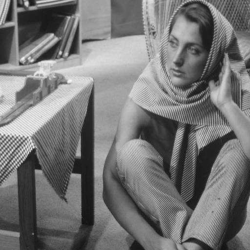
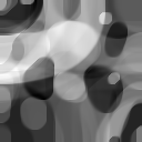
To conclude this section, we mention that scheme (S) provides an alternative decomposition into eigenfunctions in the spectral case. In the general case, however, the scheme is of limited use since it fails to decompose the whole datum, in general. Furthermore, the indecomposable rest can still contain a large amount of information as Figure 1 shows.

4 Applications
In the following, we discuss different applications for the proposed spectral decomposition scheme (S) and extinction profiles of the gradient flow (GF). After giving a short insight into the numerical computation of extinction profiles, we use the scheme and the gradient flow to compute and compare two different decompositions of an 1-dimensional signal into eigenfunctions of the total variation. Thereafter, we illustrate the use of the gradient flow and its extinction profiles for spectral graph clustering.
4.1 Numerical Computation of Extinction Profiles
Here we describe how to calculate the extinction profiles of in scheme (S). Given a time step size the solution of the gradient flow (GF) at time with datum is recursively approximated via the implicit scheme
where . These minimization problems can be solved efficiently with a primal dual optimization algorithm [8]. Defining yields a sequence of pairs where for every . Hence, in order to compute an extinction profile of , we keep track of the quantities (cf. the definition of in (4)), and define the extinction profile of as the element which has the highest Rayleigh quotient before extinction of the flow. Note that since holds for all (cf. [5]), both and, by convexity, also are in particular elements of and, thus, have a Rayleigh quotient smaller or equal than one. Hence, an extinction profile, being even an eigenfunction, can be identified by having a quotient of one. To design a criterion for extinction of the flow we make use of the fact that the subgradients in the gradient flow have monotonously decreasing norms and define the extinction time as the number such that is below a certain threshold.
4.2 1D Total Variation Example
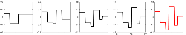
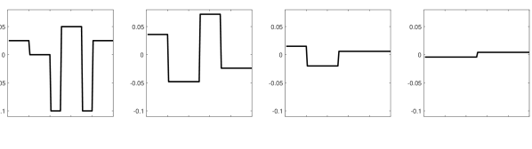
As already mentioned in Section 3, choosing to be the one-dimensional total variation yields a spectral case, i.e., the sequence in (S) weakly converges to zero which implies that is a decomposition into eigenfunctions. The rightmost images in Figure 2 show the data signal in red, whereas the other four images depict the approximation of by eigenfunctions of the gradient flow and the iterative scheme, respectively. The individual eigenfunctions (up to multiplicative constants) as computed by the gradient flow (GF) and the scheme (S) are given in Figure 3. Hence, the sum of the top four or the bottom 18 eigenfunctions, respectively, yield back the red signal from Figure 2.
Note that the gradient flow only needs four eigenfunctions to generate the data and hence gives a very sparse representation. However, the individual eigenfunctions have decreasing spatial complexity. This is a fundamental difference to the system of eigenfunctions generated by (S) which – being extinction profiles – all have low complexity. This qualitative difference can also be observed in Figure 2 where the first eigenfunction of the gradient flow (top left) already contains all the structural information of the red signal whereas the approximation in the bottom row successively adds structure.

4.3 Spectral Clustering with Extinction Profiles
Spectral clustering arises in various real world applications, e.g., in discriminant analysis, machine learning, or computer vision. The aim in this task is to partition a given data set according to the spectral characteristics of an operator that captures the pairwise relationships between each data point. Based on the spectral decomposition of this operator one tries to find a partitioning of the data into sets of strongly related entities, called clusters, that should be clearly distinguishable with respect to a chosen feature. Within each cluster the belonging data points should be homogeneous with respect to this feature.
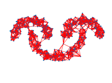
In order to model relationships between entities without further knowledge about the underlying data topology one may use finite weighted graphs. In this model each data point is represented by a vertex of the graph while the similarity between two data points is represented by a weighted edge connecting the respective vertices. For details on data analysis using finite weighted graphs we refer to [9, 12]. In the literature it is well-known that there exists a strong mathematical relationship between spectral clustering and various minimum graph cut problems. For details we refer to [17].
For the task of spectral clustering one is typically interested in the eigenvectors of a discrete linear operator known as the weighted graph Laplacian , which can be represented as a matrix of the form , for which is a diagonal matrix consisting of the degree of each graph vertex and is the adjacency matrix capturing the edge weights between vertices. Determining the discrete spectral decomposition of the graph Laplacian is a common problem in mathematics and thus easy to compute. After determining the eigenvectors of one performs the actual clustering, e.g., via a standard -means algorithm or simple thresholding. Note that in various applications a spectral clustering based on solely one eigenvector, i.e., the corresponding eigenvector of the second-smallest eigenvalue, already yields interesting results, e.g., for image segmentation [12]. On the other hand, due to the linear nature of the graph Laplacian this approach is rather restricted in many real world applications. For this reason one aims to perform spectral clustering based on eigenfunctions of a nonlinear, possibly more suitable, operator. Bühler and Hein proposed in [3] an iterative scheme to compute eigenfunctions of a nonlinear operator known as the weighted graph -Laplacian
| (8) |
Note that this operator is a direct generalization of the standard graph Laplacian for . Their idea consists in computing an eigenfunction of the linear Laplacian and use this as initialization for a non-convex minimization problem of a Rayleigh quotient which leads to an eigenfunction of with . This procedure is repeated iteratively for decreasing by using the intermediate solutions as initialization for the next step. Their method already leads to satisfying results in situations in which a linear partitioning of the given data is not sufficient. However, as the authors state themselves, this approach often converges to unwanted local minima and is restricted to eigenfunctions corresponding to the second-smallest eigenvalue.
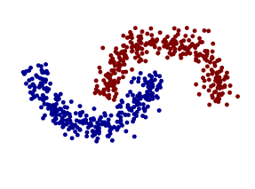
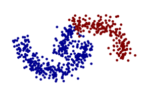
In Figure 4 we compare the spectral clustering approach from [3] based on the nonlinear graph -Laplace operator with the extinction profiles introduced in Section 2. For this we consider the following one-homogeneous, convex functional defined on vertex functions of a finite weighted graph
| (9) |
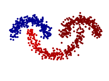
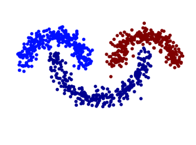
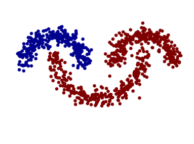
Here, denotes the weighted gradient of the vertex function in a vertex . Note that this mimics a strong formulation of TV in the continuous case. The subgradient corresponds to the graph -Laplacian as special case of the graph -Laplacian in (8) for . We test the different approaches on the “Two Moon” dataset with low noise variance (top row) and a slightly increased noise variance (bottom row). The first column shows the computed nonlinear eigenfunction by the Bühler and Hein approach. In case of low noise variance (top) the eigenfunction takes only two values and is piece-wise constant, partitioning the data well. However, the eigenfunction takes more values in the noisy case (bottom) and a subsequent -means-based clustering with does not yield a good partitioning of the data. In the center column we depict the extinction profiles computed with (GF), initialized with random values on the graph vertices. Note that both eigenfunctions are piece-wise constant and take only two values, thus inducing a binary partitioning directly. However, similar to the Bühler-Hein eigenfunction, the found eigenfunction for the noisy case is not suitable to partition the dataset correctly. Hence, we performed a third experiment in the right column in which we initialized of the nodes per cluster with the values , respectively and set the others to zero. Thus, we enforced the computation of eigenfunctions that correctly partition the data. This can be interpreted as a semi-supervised spectral clustering approach.


In conclusion we state that spectral clustering based on nonlinear eigenfunctions is a potentially powerful tool for applications in data analysis and machine learning. However, we note that neither the Bühler and Hein approach discussed above nor extinction profiles guarantee a correct partioning of the data, in general. We could mitigate this drawback by using the fact that the chosen initialization of the gradient flow influences its extinction profile.
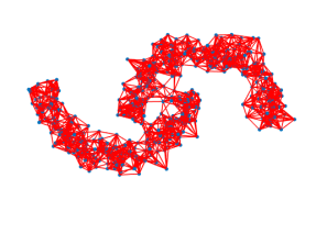
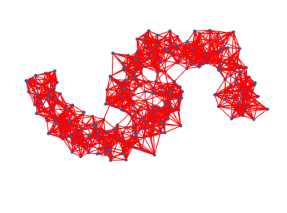
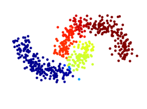
4.4 Outlook: Advanced Clustering with Higher-Order Eigenfunctions
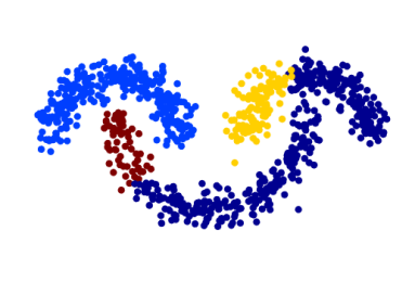
Finally, we demonstrate some preliminary results of our numerical experiments on a more challenging data set known as “Three Moons”. In this case one requires for spectral clustering an eigenfunction that is constant on each of the three half-moons. Thus, we aim to find eigenfunctions of the graph -Laplacian that correspond to a higher eigenvalue than the second-smallest one. For this reason it is apparent that Bühler and Hein’s method in its simplest variant (without subsequent splitting) always fails in this scenario (see top-right image in Figure 5). Also extinction profiles, having the lowest possible eigenvalue of all subgradients of the gradient flow (GF) lead to unreasonable results. However, one can still make use of the other subgradients and select those that are close to an eigenfunction, which can be measured by the Rayleigh quotient. The second row in Figure 5 shows three subgradients with a Rayleigh quotient of more than , as they occur in the gradient flow. Note that the last one coincides with the extinction profile and obviously fails in separating all three moons since it only computes a binary clustering. Similarly, the first subgradient finds four clusters. The correct clustering into three moons is achieved by the subgradient in the center which was the last eigenfunction to appear before the extinction profile. This underlines the need of higher-order eigenfunctions for accurate multi-class spectral graph clustering.
Acknowledgments
This work was supported by the European Union’s Horizon 2020 research and innovation programme under the Marie Skłodowska-Curie grant agreement No 777826 (NoMADS). LB and MB acknowledge further support by ERC via Grant EU FP7 – ERC Consolidator Grant 615216 LifeInverse.
References
- [1] F Andreu, Vicent Caselles, JI Diaz, and José M Mazón. Some qualitative properties for the total variation flow. Journal of Functional Analysis, 188(2):516–547, 2002.
- [2] Jean-François Aujol, Guy Gilboa, and Nicolas Papadakis. Theoretical analysis of flows estimating eigenfunctions of one-homogeneous functionals for segmentation and clustering. 2017.
- [3] Thomas Bühler and Matthias Hein. Spectral clustering based on the graph -laplacian. In International Conference on Machine Learning, pages 81–88, 2009.
- [4] Leon Bungert and Martin Burger. Solution paths of variational regularization methods for inverse problems. arXiv preprint arXiv:1808.01783, 2018.
- [5] Leon Bungert, Martin Burger, Antonin Chambolle, and Matteo Novaga. Nonlinear spectral decompositions by gradient flows of one-homogeneous functionals. arXiv preprint arXiv:1901.06979, 2019.
- [6] Martin Burger, Lina Eckardt, Guy Gilboa, and Michael Moeller. Spectral representations of one-homogeneous functionals. In International Conference on Scale Space and Variational Methods in Computer Vision, pages 16–27. Springer, 2015.
- [7] Martin Burger, Guy Gilboa, Michael Moeller, Lina Eckardt, and Daniel Cremers. Spectral decompositions using one-homogeneous functionals. SIAM Journal on Imaging Sciences, 9(3):1374–1408, 2016.
- [8] Antonin Chambolle and Thomas Pock. A first-order primal-dual algorithm for convex problems with applications to imaging. Journal of mathematical imaging and vision, 40(1):120–145, 2011.
- [9] Abderrahim Elmoataz, Matthieu Toutain, and Daniel Tenbrinck. On the -laplacian and -laplacian on graphs with applications in image and data processing. SIAM Journal on Imaging Sciences, 8(4):2412–2451, 2015.
- [10] Guy Gilboa. A total variation spectral framework for scale and texture analysis. SIAM journal on Imaging Sciences, 7(4):1937–1961, 2014.
- [11] Guy Gilboa. Nonlinear Eigenproblems in Image Processing and Computer Vision. Springer, 2018.
- [12] Zhaoyi Meng, Ekaterina Merkurjev, Alice Koniges, and Andrea L. Bertozzi. Hyperspectral image classification using graph clustering methods. Image Processing On Line, 7:218–245, 2017.
- [13] Andrew Y Ng, Michael I Jordan, and Yair Weiss. On spectral clustering: Analysis and an algorithm. In Advances in neural information processing systems, pages 849–856, 2002.
- [14] Raz Z Nossek and Guy Gilboa. Flows generating nonlinear eigenfunctions. Journal of Scientific Computing, 75(2):859–888, 2018.
- [15] Marie Foged Schmidt, Martin Benning, and Carola-Bibiane Schönlieb. Inverse scale space decomposition. Inverse Problems, 34(4):045008, 2018.
- [16] Jianbo Shi and Jitendra Malik. Normalized cuts and image segmentation. Departmental Papers (CIS), page 107, 2000.
- [17] Ulrike von Luxburg. A tutorial on spectral clustering. Statistics and Computing, 17(4):395–416, 2007.