Efficient Bayesian inference for nonlinear state space models with univariate autoregressive state equation
)
Abstract
Latent autoregressive processes are a popular choice to model time varying parameters. These models can be formulated as nonlinear state space models for which inference is not straightforward due to the high number of parameters. Therefore maximum likelihood methods are often infeasible and researchers rely on alternative techniques, such as Gibbs sampling. But conventional Gibbs samplers are often tailored to specific situations and suffer from high autocorrelation among repeated draws. We present a Gibbs sampler for general nonlinear state space models with an univariate autoregressive state equation. For this we employ an interweaving strategy and elliptical slice sampling to exploit the dependence implied by the autoregressive process. Within a simulation study we demonstrate the efficiency of the proposed sampler for bivariate dynamic copula models. Further we are interested in modeling the volatility return relationship. Therefore we use the proposed sampler to estimate the parameters of stochastic volatility models with skew Student t errors and the parameters of a novel bivariate dynamic mixture copula model. This model allows for dynamic asymmetric tail dependence. Comparison to relevant benchmark models, such as the DCC-GARCH or a Student t copula model, with respect to predictive accuracy shows the superior performance of the proposed approach.
1 Introduction
There are many situations where statistical models with constant parameters are no longer sufficient to appropriately represent certain aspects of the economy. For example it is well known that volatility of financial assets changes over time (Schwert (1989)). This is why many models that allow for variation in the parameter have been proposed. There are time varying vector autoregressive models (Primiceri (2005), Nakajima et al (2011)), stochastic volatility models (Kim et al (1998)), GAM copula models (Vatter and Chavez-Demoulin (2015), Vatter and Nagler (2018)) and many more. Stochastic volatility models and the bivariate dynamic copula model of Almeida and Czado (2012) assume that the parameter follows a latent autoregressive process of order 1 (AR(1) process). These two models belong to the class of models that we will study.
In a general time varying parameter framework we consider a dimensional random variable at time , , which is generated from a dimensional density . We are interested in models, where the density has a univariate dynamic parameter following an AR(1) process. These models can be formulated as state space models with observation equation
| (1) |
for . The state equation describes an AR(1) process with mean parameter , persistence parameter and standard deviation parameter and is given by
| (2) |
where for and . In the state equation we assume Gaussian innovations but in the observation equation we do not put any restrictions on the density . Thus we allow for nonlinear and non Gaussian state space models. Several established models can be analyzed within this framework.
By choosing as the univariate normal density with mean and variance , denoted by , we obtain the stochastic volatility model (Kim et al (1998)) given by
| (3) |
for . By modeling the log variance as a latent AR(1) process this model allows for time varying volatility. Time varying volatility is a stylized fact of financial time series. In this context, the stochastic volatility model has also shown better performance than the frequently used GARCH models (Engle (1982), Bollerslev (1986)) for several data sets (Yu (2002), Chan and Grant (2016)). To allow for heavy tails and skewness, other distributions have been considered in the observation equation. One example is the stochastic volatility model with skew Student t errors (Abanto-Valle et al (2015)), which can also be analyzed within our framework.
Dependence modeling is another research area, where models that allow for time varying parameters have been introduced. Vine copulas (Bedford and Cooke (2001), Aas et al (2009), Czado (2019)) are widely used models to capture complex dependence structures. To name a few, Brechmann and Czado (2013) and Nagler et al (2019) employ vine copulas for forecasting the value at risk of a protfolio, Aas (2016) gives an overview of applications of vine copulas in finance including asset pricing, credit risk management and portfolio optimization and Barthel et al (2018) model the association pattern between gap times with D-vine copulas to study asthma attacks. A vine copula model is made up of different bivariate copulas with corresponding dependence parameters. Since dependencies may change over time, extensions that allow for variation in the dependence parameter have been proposed. Vatter and Chavez-Demoulin (2015) introduce a bivariate copula model, where the dependence parameter follows a generalized additive model. Another approach is the dynamic bivariate copula model proposed by Almeida and Czado (2012) and Hafner and Manner (2012), which we will analyze within our state space framework. For this model, we consider single parameter copula families for which there is a one-to-one correspondence between the copula parameter, denoted by , and Kendall’s . So we can express Kendall’s as a function of the copula parameter and we write . The restriction of Kendall’s to the interval is removed by applying the Fisher’ Z transformation . This transformed time varying Kendall’s is then modeled by an AR(1) process. More precisely, we consider bivariate random vectors, , corresponding to time points. We assume for that
| (4) |
where is a bivariate copula density with parameter .
Nonlinear state space models as specified with (1) and (2) are typically difficult to estimate, since there is a large number of parameters and likelihood evaluation requires high dimensional integration. This often makes maximum likelihood approaches infeasible. Gibbs sampling (Geman and Geman (1984)) is a frequently used Bayesian approach to infer parameters of such nonlinear state space models (Carlin et al (1992)). But the posterior samples, resulting from conventional Gibbs sampling, often suffer from high autocorrelation. Furthermore, the availability of the full conditional distributions or at least an efficient MCMC approach to sample from them is required. This is often tailored to specific situations. We present a Gibbs sampling approach that is designed to handle models with a latent AR(1) process and general likelihood functions as specified by the state space formulation in Equations (1) and (2). To sample from the associated posterior distribution we rely on elliptical slice sampling (Murray et al (2010)) and on an ancillarity-sufficiency interweaving strategy (Yu and Meng (2011)). Elliptical slice sampling is used to sample the latent states. This allows us to exploit the Gaussian dependence structure, that is implied by the AR(1) process. But even if we provide efficient methods to sample from the full conditionals, the sampler may still suffer from the dependence among the parameters in the posterior distribution. Additionally, its performance may vary for different model parameterizations (Frühwirth-Schnatter and Sögner (2003), Strickland et al (2008)). This problem is tackled with the ancillarity-sufficiency interweaving strategy, where the parameters of the latent AR(1) process are sampled from two different parameterizations. The decision between two parameterizations is avoided by using both. This approach has already shown good results for several models, including univariate and multivariate stochastic volatility models (Kastner and Frühwirth-Schnatter (2014), Kastner et al (2017)). The efficiency of our proposed sampler is illustrated with a simulation study.
The second part of this work has a more applied focus and deals with modeling the volatility return relationship, i.e. the dependence between an index and the corresponding volatility index. More precisely, we investigate the American index SP500 and its volatility index the VIX as well as the German index DAX and the VDAX. It is important to provide appropriate models for this relationship, since it has influence on hedging and risk management decisions (Allen et al (2012)). For our analysis we make use of a two step approach commonly used in copula modeling (Joe and Xu (1996)) motivated by Sklar’s Theorem (Sklar (1959)). We first model the marginal distribution with a univariate skew Student t stochastic volatility model. In the second step we model the dependence for which we propose a dynamic copula model allowing for asymmetric tail dependence. This model is a dynamic mixture of a Gumbel and a Student t copula and can be seen as an alternative to the symmetrized Joe-Clayton copula of Patton (2006). Estimation is carried out through a two step approach, where we first estimate the marginal stochastic volatility models, fix their parameters at point estimates and then estimate the dynamic mixture copula. At both steps, estimation is straightforward with the proposed sampler. Our model is able to capture several characteristics of the joint distribution of volatility and return. With respect to the marginal distribution we observe positive skewness for volatility indices compared to slight negative skewness for the return indices. In the dependence structure we identify asymmetry and time variation. Finally, we compare the proposed model to several restricted models with constant or symmetric dependence and to a bivariate DCC-GARCH model (Engle (2002)). Model comparison with respect to predictive accuracy shows the superiority of our approach.
To summarize, the main contribution of this paper is an approach to efficiently sample from the posterior distribution of general nonlinear state space models as specified by Equations (1) and (2). In addition, we propose a dynamic mixture copula for time varying asymmetric tail dependence. We discuss Bayesian inference for this model class and demonstrate how it can be utilized to model the volatility return relationship.
The outline of the paper is as follows: After the introduction, we discuss the proposed MCMC approach in Section 2. In Section 3 we investigate the efficiency of the sampler for bivariate dynamic copula models through an extensive simulation study. Section 4 deals with modeling the volatility return relationship and Section 5 concludes.
2 Bayesian inference
In the following, we denote an observation of the -dimensional random vector by and the associated data matrix is given by . To subset vectors and matrices we make use of the following notation: For sets of indices and we set for a vector and for a matrix . We use a capital letter to refer to a matrix and small letters to refer to its components. The set of integers will be abbreviated by .
We consider the state space model as specified by Equations (1) and (2). To obtain a fully specified Bayesian model we equip the parameters , and with prior distributions. We follow Kastner and Frühwirth-Schnatter (2014), who propose the following prior distributions for the latent AR(1) process of the stochastic volatility model:
| (5) |
where . Our standard choice for the prior hyperparameters is and as in Kastner (2016). With these prior distributions our Bayesian model is complete. For sampling from the posterior distribution of this model we should take into account that sampling efficiency may highly depend on the model parameterization (Frühwirth-Schnatter and Sögner (2003), Strickland et al (2008)). Yu and Meng (2011) differentiate between two parameterizations: A sufficient augmentation and an ancillary augmentation scheme. In our case a sufficient augmentation is characterized by an observation equation that is free of the parameters and and only depends on the latent states . In this case is a sufficient statistics for the parameters and . In an ancillary augmentation the state equation is independent of the parameters and , then is an ancillary statistics for the parameters and . The standard parameterization of our model is already a sufficient augmentation and we refer to this parameterization as given by Equations (1) and (2) as (SA).
An ancillary augmentation is obtained by the following parameterization
| (6) |
for . This reparameterization is obtained by solving Equation (2) for and implies that the state space model is given by
where is the function that calculates according to (6). We refer to this model representation as (AA). Instead of deciding between (SA) and (AA), we combine them in an ancillarity-sufficiency interweaving strategy (Yu and Meng (2011)), given by
-
•
a) Sample in (SA) from .
-
•
b) Sample in (SA) from .
-
•
c) Move to (AA) via for .
-
•
d) Sample in (AA) from .
-
•
e) Move back to (SA) via the recursion for .
Kastner and Frühwirth-Schnatter (2014) employed interweaving for the stochastic volatility model and showed its superior performance with an extensive simulation study. For the stochastic volatility model, Kastner and Frühwirth-Schnatter (2014) propose to move between a sufficient augmentation and a reparameterization of the latent states given by . Within this reparameterization parameters can be sampled conveniently from its full conditional distribution by recognizing a linear regression model. This is possible for the standard stochastic volatility model, but not in our case since our sampler is designed to handle more general likelihood functions. Therefore we have chosen the reparameterization of (SA) such that it is optimal in the sense of Yu and Meng (2011), i.e. we move between a sufficient and a ancillary augmentation.
Note that reducing the sampler to the first two steps a) and b) results in a standard Gibbs sampler in (SA). This sampler typically suffers from the dependence among the parameters and the latent states in the posterior distribution.
Step a: Sampling of the latent states in the sufficient augmentation
To sample the latent states from its full conditional in (SA) we make use of elliptical slice sampling as proposed by Murray et al (2010). It was developed for models, where dependencies are generated through a latent multivariate normal distribution. In (SA), the AR(1) structure implies, that the vector has a dimensional multivariate normal distribution with mean vector and covariance matrix given by
| (7) |
(see e.g. Brockwell et al (2002), Chapter 2.2). The posterior density is proportional to
where and are given in (7) and denotes the corresponding prior density as specified in (5). The initial state can be sampled from its full conditional density given by
The full conditional density of the latent states is given by
with a corresponding mean vector and covariance matrix . The mean vector and the covariance matrix of the conditional distribution are derived in a more general way in Appendix A. By reparameterizing the model with we impose a multivariate normal prior with zero mean. We obtain the situation elliptical slice sampling was designed for. However updating the whole dimensional vector with elliptical slice sampling at once will lead to high autocorrelation in the posterior draws. This is illustrated in Section 3 and was also observed by Hahn et al (2019), where elliptical slice sampling was used for linear regression models. Hahn et al (2019) circumvent this problem by partitioning the vector into smaller blocks. We follow this approach and partition the set into different blocks . Let denote the minimal and denote the maximal index in the -th block. The blocks are chosen such that , for . The full conditional density for the -th block can be expressed as where . The vector is multivariate normal distributed with mean denoted by and covariance matrix (see Appendix A) and therefore the full conditional density can be written as
To sample the latent states of the -th block from its full conditional we proceed as follows
-
•
Set
-
•
Draw from the density
using elliptical slice sampling, where is interpreted as the prior density for .
-
•
Set
Step b: Sampling of the constant parameters in the sufficient augmentation
In (SA) the observation equation only depends on and is independent of the parameters , and . The parameters , and only depend on . This allows to use the same approach as in Kastner and Frühwirth-Schnatter (2014) to sample the parameters and in (SA). We reparameterize the model such that proposals can be found using Bayesian linear regression. We define and the state equation is given by
where . For fixed , this is a linear regression model with regression parameters and variance . Proposals for are found and accepted or rejected as described in Kastner and Frühwirth-Schnatter (2014) Section 2.4 (two block sampler).
Step d: Sampling of the constant parameters in the ancillary augmentation
To sample and in (AA) we deploy a random walk Metropolis-Hastings scheme with Gaussian proposal, where the proposal variance or covariance matrix is adapted during the burn-in period. For the adaptions we use the Robbins Monro process (Robbins and Monro (1985)) as suggested by Garthwaite et al (2016). More details are given in Appendix A.
Implementation
For the implementation of the sampler we use Rcpp (Eddelbuettel et al (2011)) which allows to embed C++ code into R. In addition we make use of rvinecopulib (Nagler and Vatter (2018)) to evaluate copula densities and of RcppEigen (Bates et al (2013)). For sampling in (SA) we use corresponding parts of the implementation of the R package stochvol (Kastner (2016)). The R package coda (Plummer et al (2008)) is used to compute effective sample sizes in the following section.
3 Illustration of the proposed sampler for bivariate dynamic copula models
We illustrate the MCMC sampler we proposed in the previous section for the bivariate dynamic copula model of Almeida and Czado (2012). Kastner and Frühwirth-Schnatter (2014) have already shown that interweaving improves sampling efficiency a lot for the stochastic volatility model. We investigate if this is also the case for the bivariate dynamic copula model. Further we study how the sampling efficiency is affected by the chosen block size and by the data generating process (DGP). Therefore we perform an extensive simulation study. We consider different modifications of the sampler. A sampler is specified by a vector which indicates its blocksize (b) and if interweaving is used (i=I) or not (i=NI). We consider ten different sampler specifications , where is the length of the time series. By using blocks of size , we obtain the sampler which updates the parameters jointly with elliptical slice sampling. If we turn off interweaving (i=NI) we obtain a standard Gibbs sampler updating parameters in the sufficient augmentation. These samplers are run for different simulated data sets. A data set is simulated from the bivariate dynamic copula model (see (4)) with parameters: Family, . The parameters are chosen from the following grid (Family, ) . Here, eClayton denotes the extended Clayton copula, which extends the Clayton copula to allow for negative Kendall’s values. More precisely, the extended Clayton copula has the following density
where is the density of the bivariate Clayton copula with parameter (see Joe (2014), Chapter 4). So the extended Clayton copula density is equal to the Clayton copula density for non negative Kendall’s and equal to a 90 degree rotation of the Clayton copula density for negative Kendall’s . Among the different DGPs, most distinct values are considered for . We expect its choice to be influential since it controls the dependence among the latent variables. With this grid we obtain 180 different DGPs. For each of the different DGPs we generate 100 simulated data sets and for each data set we run the 10 different samplers with the correctly specified copula family for 25000 iterations and discard the first 5000 iterations for burn-in. So, in total we obtain 18000 simulated data sets and each of the 10 samplers is run 18000 times.
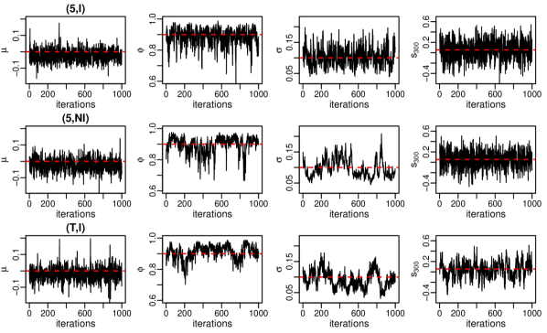
Figure 1 shows trace plots of different parameters (, , , ) based on one simulated data set for three different sampler specifications. We consider specification (5,I), and the same specification with interweaving turned off, i.e. (5,NI) and the specification (T,I). We observe that all three samplers produce posterior samples covering the true values. Further, the trace plots suggest that the (5,I) sampler achieves better mixing than the other two considered samplers.
The runtime of the sampler is mainly affected by the choice of and the sampler specification. From Table 1 we see that the runtime is increasing in and that interweaving adds considerable additional runtime.
| (1,I) | (5,I) | (20,I) | (100,I) | (T,I) | (1,NI) | (5,NI) | (20,NI) | (100,NI) | (T,NI) | |
|---|---|---|---|---|---|---|---|---|---|---|
| 0.6 | 0.5 | 0.5 | 0.7 | 0.8 | 0.3 | 0.3 | 0.3 | 0.4 | 0.5 | |
| 1.1 | 1.0 | 1.1 | 1.3 | 1.6 | 0.7 | 0.5 | 0.6 | 0.8 | 1.1 | |
| 1.7 | 1.4 | 1.6 | 1.9 | 2.6 | 1.0 | 0.7 | 0.9 | 1.2 | 1.8 |
To measure efficiency of the samplers we consider the effective sample size per minute which we call effective sampling rate, similar to Hosszejni and Kastner (2019). We average the effective sampling rate of 100 runs, where the same sampler and the same DGP was used. Then we obtain 180 average effective sampling rates (AESR) per sampler. Since the AESR decreases for higher values of for every sampler, we compare the ten different samplers among DGPs with the same value for . For a fixed we have 60 AESR values per sampler. For each sampler, the minimum of these 60 values (mAESR) is given in Table 2. We consider the minimum since we are interested in samplers that are reliable for all DGPs. We see that for the parameters , and sampler specifications with interweaving have higher mAESR values, while for the latent states specifications without interweaving perform better. Although interweaving adds additional runtime, it still increases the mAESR of , and considerably. Further we observe that choosing the blocksize too big results in very low mAESR values for the latent states. In this case many parameters are updated jointly with elliptical slice sampling which results in high autocorrelation among consecutive draws. The performance of samplers with blocksize is especially poor. For these samplers the length of the time series ( 500, 1000, 1500) also has strong effects. For example the mAESR for for specification (T,NI) decreases by 85 from 78 to 11 when the length of the time series is increased from 500 to 1500. The most inefficient sampler is (T,NI), the sampler without interweaving and with the largest blocksize. In our opinion the best results are obtained for sampler specification (5,I). It provides the highest mAESR values for , and for all choices of and also provides rather high mAESR values for the latent states.
| (1,I) | (5,I) | (20,I) | (100,I) | (T,I) | (1,NI) | (5,NI) | (20,NI) | (100,NI) | (T,NI) | |
| 2829 | 3178 | 1813 | 642 | 381 | 437 | 838 | 780 | 277 | 78 | |
| 471 | 749 | 556 | 191 | 60 | 266 | 326 | 232 | 78 | 24 | |
| 272 | 411 | 263 | 58 | 33 | 53 | 74 | 56 | 23 | 6 | |
| (a) | 938 | 2982 | 2484 | 199 | 36 | 1347 | 4942 | 3908 | 273 | 49 |
| (m) | 346 | 1092 | 441 | 35 | 5 | 496 | 1011 | 627 | 41 | 5 |
| 1167 | 1365 | 840 | 309 | 180 | 172 | 330 | 371 | 121 | 21 | |
| 202 | 269 | 212 | 73 | 17 | 81 | 97 | 76 | 27 | 6 | |
| 97 | 175 | 133 | 25 | 9 | 18 | 25 | 21 | 12 | 1 | |
| (a) | 298 | 1011 | 1312 | 99 | 12 | 400 | 1911 | 1982 | 133 | 16 |
| (m) | 115 | 417 | 200 | 15 | 1 | 161 | 559 | 296 | 17 | 2 |
| 711 | 833 | 578 | 200 | 111 | 89 | 218 | 231 | 75 | 11 | |
| 120 | 145 | 107 | 43 | 9 | 38 | 49 | 42 | 14 | 3 | |
| 63 | 109 | 84 | 16 | 3 | 10 | 14 | 13 | 8 | 1 | |
| (a) | 162 | 583 | 879 | 66 | 7 | 247 | 1168 | 1359 | 90 | 10 |
| (m) | 61 | 239 | 112 | 9 | 1 | 95 | 426 | 176 | 11 | 1 |
In addition to the previous analysis, we investigate how different DGPs affect the samplers. Therefore we consider the best sampler according to Table 2, i.e. sampler specification (5,I). In addition we have a look at the same sampler specification without interweaving (5,NI) and the same sampler with joint updates of the latent states, i.e. (T,I). We consider the AESR for , which is usually the parameter which causes most problems. Table 3 shows for each of these three samplers the DGPs with which resulted in the lowest and the highest AESR for . For the (5,I) specification satisfactory AESR values, ranging from 175 to 456, are obtained for all DGPs. In the (T,I) specification the latent states are updated jointly. In scenarios with strong dependence among the latent states ( = 0.99) this sampler performs poorly whereas the best performance of the sampler was seen for a DGP with low dependence among the latent states (=0). The (5,NI) specification is a standard Gibbs sampler in the sufficient augmentation. We see that for this specification the AESR values vary a lot, ranging from 25 to 558. The best performance of this sampler specification was seen for a DGP with high persistence (). Kastner and Frühwirth-Schnatter (2014) studied different sampling schemes for the stochastic volatility model and have also seen that a standard Gibbs sampler in the sufficient augmentation performs well for scenarios with high persistence.
| (5,I) | (T,I) | (5,NI) | |||||
| AESR() | min | max | min | max | min | max | |
| 175 | 456 | 9 | 121 | 25 | 558 | ||
| DGP | family | Gauss | eClayton | eClayton | eClayton | Gauss | eClayton |
| 0 | 1 | 0 | 0 | 0 | 0 | ||
| 0.1 | 0.9 | 0.99 | 0 | 0.1 | 0.99 | ||
| 0.2 | 0.2 | 0.2 | 0.05 | 0.05 | 0.2 | ||
Lastly we compare our sampler to the coarse grid sampler employed by Almeida and Czado (2012). We already covered six DGPs that were also analyzed by Almeida and Czado (2012). Instead of running their sampler we make the comparison with respect to these six cases. There are several points which make the comparison slightly less reliable. First Almeida and Czado (2012) did not report exact computation times but they note that 100 000 iterations of their sampler take about 15 minutes. We use this number to calculate the AESR values from the effective sample sizes they report in their paper. Second their calculations were performed on a different computer and third they use different prior distributions for and . But we think that this comparison should still give us a rough idea of how the sampling efficiencies compare to each other. From Table 4 we see that the (5,I) specification considerably outperforms the coarse grid sampler (CG). For every parameter (, , ) we obtain way higher AESR values.
| DGP | AESR() | AESR() | AESR() | ||||||
|---|---|---|---|---|---|---|---|---|---|
| family | (5,I) | CG | (5,I) | CG | (5,I ) | CG | |||
| Gauss | 8187 | 2130 | 527 | 81 | 393 | 50 | |||
| Gauss | 1637 | 305 | 364 | 83 | 437 | 69 | |||
| Gauss | 9935 | 4150 | 549 | 150 | 316 | 85 | |||
| eClayton | 8382 | 2088 | 539 | 74 | 397 | 46 | |||
| eClayton | 1778 | 279 | 378 | 71 | 416 | 52 | |||
| eClayton | 10079 | 4375 | 574 | 175 | 323 | 97 | |||
4 Application: Modeling the volatility return relationship
We investigate the volatility return relationship through the bivariate joint distribution of a stock index and the corresponding volatility index. The joint distribution of return and volatility incorporates all the marginal information as well as information about the dependence, which are both relevant for hedging and risk management (Allen et al (2012)). Since there has already been evidence for asymmetry in the joint distribution of volatility and return (Allen et al (2012), Fink et al (2017)) models which are able to handle these characteristics are necessary.
The two step copula modeling approach motivated by Sklar’s theorem (Sklar (1959)) provides a very flexible method for the construction of multivariate distributions. We can combine arbitrary marginal distributions with any copula. Here, we propose a bivariate model that combines the skew Student t stochastic volatility model (Abanto-Valle et al (2015)) for the margins with a novel dynamic mixture copula. This model allows for asymmetry and heavy tails in the marginal distribution as well as for time varying asymmetric tail dependence in the dependence structure. Both, the marginal as well as the copula model can be estimated with the proposed sampler.
Marginal model
The stochastic volatility model with skew Student t errors is obtained by replacing the normal distribution of the stochastic volatility model (Kim et al (1998)) by a skew Student t distribution. This allows for heavy tails and skewness. The stochastic volatility model with skew Student t errors as considered by Abanto-Valle et al (2015) is given by
| (8) |
where independently for . We denote by the density of the standardized skew Student t distribution with parameters and (cf. Appendix B). Compared to our framework this model has two additional parameters and . For these additional parameters we choose the following prior distributions
| (9) |
where denotes the normal distribution truncated to . We need to ensure that since the standardized skew Student t distribution would not be well defined otherwise.
Conditional on and our sampler can be applied directly to sample from its full conditional. Another approach, which lead to better mixing, is to include the parameters and in the interweaving strategy. The sampler is slightly modified in the following way:
-
•
a) Sample from .
-
•
b) Sample in (SA) from .
-
•
c) Move to (AA) via for .
-
•
d) Sample in (AA) from .
-
•
e) Move back to (SA) via the recursion for .
For step a) we proceed as described in Section 2. For step b) we draw and from its univariate full conditional distributions using Metropolis-Hastings, similar to Step d) in Section 2. The parameters are drawn from its full conditional as described in Section 2. For step d) we investigated different blocking strategies for the parameters . We compared the different strategies with respect to effective sample sizes and decided to use the following three blocks: and . Each block is updated using Metropolis-Hastings as in Step d) in Section 2.
Dependence model
Dependence among financial assets is often modeled with a Student t copula. This copula allows for tail dependence symmetric in the upper and lower tail. Evidence against the assumption of symmetric tail dependence has been provided and models to handle this characteristic have become necessary (Patton (2006), Nikoloulopoulos et al (2012), Jondeau (2016)). Patton (2006) proposes the symmetrized Joe-Clayton copula. This is a modification of the BB7 copula (Joe (2014), Chapter 4) that is symmetric if upper and lower tail dependence coincide, which he describes as a desirable property. In the application of Nikoloulopoulos et al (2012) the Student t copula provides the best fit in terms of the likelihood. But they argue that if the focus is on the tails a BB1 or BB7 copula might be more appropriate. The BB1 and BB7 copulas have two parameters which might not be enough, if we want to model three characteristics in a flexible way: upper tail dependence, lower tail dependence and overall dependence as measured with Kendall’s . We provide another approach to relax the symmetric tail dependence assumption. We propose a mixture of a Student t and a extended Gumbel copula with parameters , and given by
| (10) |
where is the bivariate Student t copula specified by Kendall’s and the degree of freedom and is the bivariate extended Gumbel copula specified by Kendall’s . The extended Gumbel copula is defined similarly to the extended Clayton copula in Section 2, i.e. its density is equal to the Gumbel copula density for positive values of Kendall’s and equal to a 90 degree rotation of the Gumbel copula density for negative Kendall’s values. Both copulas and share the dependence parameter and we expect the mixture copula to have a similar strength of dependence. The corresponding Kendall’s of the mixture copula is given by
| (11) |
We evaluated the integral in (11) numerically for different values of , and and observed only negligible difference between and . The upper and lower tail dependence coefficients and of the mixture copula can, for , be obtained as
where we used the well known formulas for the tail dependence coefficients of the Student t and the Gumbel copula (Joe (2014), Chapter 4). Whereas the upper and lower tail dependence coefficients measure dependence in the upper right and lower left corner, we are also interested in the dependence in the upper left and the lower right corner when . We consider the following tail dependence coefficients in the upper left corner and in the lower right corner if
analogous to the definition of quarter tail dependence in Fink et al (2017).
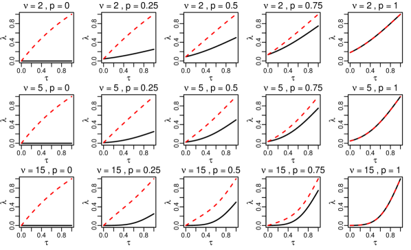
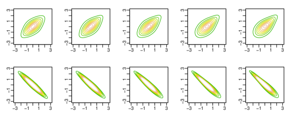
The tail dependence coefficient of the mixture copula is a linear combination of the tail dependence coefficients of its two components, the Student t and the Gumbel copula. The Student t copula has symmetric tail dependence, whereas the Gumbel copula has upper but no lower tail dependence. So we expect upper tail dependence to be higher than lower tail dependence in the mixture copula. The amount of asymmetry in the tails is controlled by , whereas the copula is symmetric in the tails for and the level of asymmetry increases as we decrease . So this copula allows for great flexibility: The overall dependence can be described by Kendalls’s , the degrees of freedom parameter controls the upper and lower tail dependence coefficient and controls the difference between upper and lower tail dependence. This is visualized in Figure 4 in Appendix C. Note that the desirable property according to Patton (2006) of symmetry in case of coinciding upper and lower tail dependence is here fulfilled. If we expected higher lower than upper tail dependence we can replace the Gumbel copula by a survival Gumbel copula which has the density . To allow for time variation we use the mixture copula of (10) within the dynamic bivariate copula model of Almeida and Czado (2012). A nonlinear state space model for bivariate random vectors , corresponding to time points, is given by
| (12) |
for . We assign a uniform prior on for , a normal prior with mean 5 and standard deviation 20 truncated to the interval for and the same priors as in (5) for the remaining parameters. Sampling is done in the following way.
-
•
Draw and from its univariate full conditionals with random walk Metropolis-Hastings with Gaussian proposal (proposal standard deviation: 0.3).
-
•
Draw conditioned on and as in Section 2.
Two step estimation
We consider the SP500 (SPX) and its volatility index the VIX as well as the DAX and its volatility index the VDAX. The daily log returns from 2006 to 2013 of these indices are obtained from Yahoo finance (https://finance.yahoo.com). With approximately 250 trading days per year this results in 2063 observations, visualized in Figure 6 in Appendix D. The corresponding data matrix with 2063 rows and 4 columns is denoted by .
Combining the marginal and the dependence model we obtain that for bivariate random vectors the following holds
| (13) |
independently, where
and iid, as in (9), as in (12) and , , , , , , , as in (2) and (5) for and . Here, denotes the distribution function of the standardized skew Student t distribution (cf. Appendix B). We refer to the probability integral transforms and for as copula data.
For inference we rely on a two step approach. We first estimate marginal distributions and based on the resulting estimated copula data we estimate the copula parameters. This approach is also called inference for margins (Joe and Xu (1996)) and is commonly used in (Bayesian) copula modeling (Min and Czado (2011), Almeida and Czado (2012), Smith (2015), Gruber et al (2015), Loaiza-Maya et al (2018)).
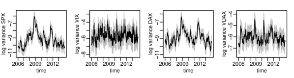
First we fit a skew Student t stochastic volatility model for each of the indices. For each index we run the sampler (5,I) for 31000 iterations and discard the first 1000 draws as burn-in. As it is typical for financial data all indices show a high persistance parameter (Posterior mode estimates for : SPX: , VIX: , DAX: , VDAX: ). A notable difference is that for stock indices we observe negative skewness, whereas for the volatility indices positive skewness is observed (Posterior mode estimates for : SPX: , VIX: , DAX: , VDAX: ). Evidence for negative skewness has also been observed for the log returns of other stock indices, as e.g., for the NASDAQ by Abanto-Valle et al (2015). Posterior mode estimates, posterior quantiles and effective samples sizes for several parameters of the four marginal models are summarized in Table 7 in Appendix D. The estimated daily log variances are shown in Figure 2. In the end of 2009, the estimated variances are high for all indices due to the financial crisis.
In the next step we obtain data on the [0,1] scale by applying the probability integral transform using the posterior mode estimates of the marginal parameters. We refer to this data as pseudo copula data and it is obtained as
where are the posterior mode estimates of the corresponding marginal skew Student t stochastic volatility model for . In the copula data marginal characteristics are removed and what is left is information about the dependence structure. Based on the pseudo copula data two dynamic mixture copula models are fitted, one corresponding to the pair (SPX,VIX) and one corresponding to the pair (DAX,VDAX). For each pair we obtain 31000 iterations with the sampler specification (5,I) and discard the first 1000 draws as burn-in. The posterior mode estimates for are for the model for (SPX,VIX) and for the model for (DAX,VDAX), respectively. (Further, posterior statistics for the model parameters and are shown in Table 8 in Appendix D). So both fitted models allow for asymmetric tail dependence, whereas the asymmetry is stronger for the (SPX,VIX) model. For these models tail dependence in the upper left corner is stronger than the one in the lower right corner . This means that joint extreme comovements, where the stock index decreases and the volatility index increases are more likely to occur than vice versa, which agrees with the statement that the market reacts more extreme in bad market situations (Sun and Wu (2018)).
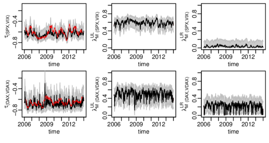
The time varying estimates for Kendall’s and the tail dependence coefficients are shown in Figure 3. The figure visualizes the asymmetry in tail dependence. We also observe changes in tail dependence as time evolves: for (SPX,VIX), ranges from to and from to . For the pair (DAX,VDAX), ranges from to and from to . This variation over time in tail dependence goes hand in hand with variation in Kendall’s . For (SPX,VIX), Kendall’s ranges from to and for (DAX,VDAX) from to .
Out of sample predictions
We aim to further support the findings we obtained through the dynamic copula model, i.e. that the dependence structure is asymmetric and varies over time. Therefore we consider several restrictions with respect to the dependence structure. Giving up time variation leads a constant mixture copula, giving up asymmetry leads to a dynamic Student t copula and giving up time variation and asymmetry leads to a constant Student t copula. In addition, we compare our model to the frequently used dynamic conditional correlation (DCC) GARCH model of Engle (2002). The DCC-GARCH allows for time varying symmetric dependence. So we take five different models into consideration. These models are summarized in Table 5. The model is the model given in (13), which was also used for the previous analysis.
We compare the models with respect to cumulative pseudo log predictive scores (Kastner (2019)), which are obtained by evaluating the corresponding density at point estimates, instead of averaging over all posterior draws. In comparison to other multivariate scoring rules, such as the energy score or the variogram score (Scheuerer and Hamill (2015)), pseudo log predictive scores have here the advantage that they can be computed fast since they require only one evaluation of the density per observation. We consider observations of dimension two, stored in the data matrix , where the first observations are used to train the model and the last are used for testing.
| model | specification | margin | dependence | |
|---|---|---|---|---|
| asymmetric | asymmetric | dynamic | ||
| sstSV + dynamic mixture copula | Yes | Yes | Yes | |
| sstSV + constant mixture copula | Yes | Yes | No | |
| sstSV + dynamic Student t copula | Yes | No | Yes | |
| sstSV + constant Student t copula | Yes | No | No | |
| DCC(1,1)-GARCH(1,1) | No | No | Yes | |
The DCC-GARCH model is estimated based on data points in the training period. Based on this model, we obtain rolling one-day ahead estimates of the covariance matrix for each day in the test set. The pseudo log predictive scores are obtained by evaluating the corresponding multivariate normal log densities at the observations. To estimate the DCC-GARCH models we used the R package rmgarch of Ghalanos (2012).
Similarly, the model is estimated with the training data. Instead of computing daily updates for all model parameters we fix the constant parameters at their posterior mode estimates to save computation time. The dynamic parameters are updated daily and the one-day ahead forecasts are obtained by evolving the AR(1) process. To obtain the pseudo log predictive scores we evaluate the density implied by (13) at the corresponding observations. Appendix D contains a detailed description of this procedure. The pseudo log predictive scores for , and are obtained similarly.
This procedure for calculating the pseudo log predictive scores is applied for both data sets corresponding to the pairs (SPX,VIX) and (DAX,VDAX). Using the last two years (2012 - 2013) of our data set as test data yields . As training period we use which corresponds to a training period of approximately four years.
Table 6 summarizes the cumulative pseudo log predictive scores. In both cases, for the (SPX,VIX) as well as for the (DAX,VDAX) data, the best model is provided by the dynamic mixture copula model . Furthermore, we see that in both cases the constant mixture copula model is preferred over the constant and dynamic Student t copula models and . For the (DAX,VDAX) data, the second best model is provided by the constant mixture copula model . For this data the rolling window estimates of Kendall’s in Figure 3 vary less than for the (SPX,VIX) data. For the (SPX,VIX) data, the DCC-GARCH yields the second best cumulative pseudo log predictive scores.
| (SPX,VIX) | 2740.7 | 2733.5 | 2732.0 | 2725.9 | 2737.2 |
| (DAX,VDAX) | 2817.7 | 2814.1 | 2810.1 | 2809.9 | 2789.0 |
5 Conclusion
We propose a sampler, applicable to general nonlinear state space models with univariate autoregressive state equation. Sampling efficiency is demonstrated for bivariate dynamic copula models within a simulation study. Furthermore we use the sampler to estimate the parameters of a dynamic bivariate mixture copula model. This mixture copula model turns out to be a good candidate to model the volatility return relationship, since in our application it produces more accurate forecasts than a bivariate DCC-GARCH model or a Student t copula model.
In this work, there are two objectives that might be extended: The sampler and the bivariate mixture copula model. The sampler could be extended to allow for a broader class of models. For example we might consider autoregressive processes of higher order in the state equation. In this case we can still rely on elliptical slice sampling and on an interweaving strategy. Another extension could relax the assumption of a Gaussian dependence structure in the state equation by replacing the autoregressive process by a D-vine copula model. In this case elliptical slice sampling can no longer be applied to sample the latent states and an alternative sampling method is required.
The bivariate dynamic mixture copula could serve as a building block for regular vine copula models. Thus we could extend the bivariate model to arbitrary dimensions. This is interesting if we study not only the bivariate volatility return relationship, but for example the dependence structure among several exchange rates.
References
- Aas (2016) Aas K (2016) Pair-copula constructions for financial applications: A review. Econometrics 4(4):43
- Aas et al (2009) Aas K, Czado C, Frigessi A, Bakken H (2009) Pair-copula constructions of multiple dependence. Insurance: Mathematics and Economics 44(2):182–198
- Abanto-Valle et al (2015) Abanto-Valle C, Lachos V, Dey DK (2015) Bayesian estimation of a skew-student-t stochastic volatility model. Methodology and Computing in Applied Probability 17(3):721–738
- Allen et al (2012) Allen D, Singh A, Powell R, McAleer M, Taylor J (2012) The Volatility-Return Relationship: Insights from Linear and Non-Linear Quantile Regressions. School of Accounting. Finance and Economics & FEMARC Working Paper Series
- Almeida and Czado (2012) Almeida C, Czado C (2012) Efficient Bayesian inference for stochastic time-varying copula models. Computational Statistics & Data Analysis 56(6):1511–1527
- Azzalini and Capitanio (2003) Azzalini A, Capitanio A (2003) Distributions generated by perturbation of symmetry with emphasis on a multivariate skew t-distribution. Journal of the Royal Statistical Society: Series B (Statistical Methodology) 65(2):367–389
- Barthel et al (2018) Barthel N, Geerdens C, Czado C, Janssen P (2018) Dependence modeling for recurrent event times subject to right-censoring with D-vine copulas. Biometrics 75:439–451
- Bates et al (2013) Bates D, Eddelbuettel D, et al (2013) Fast and elegant numerical linear algebra using the RcppEigen package. Journal of Statistical Software 52(5):1–24
- Bedford and Cooke (2001) Bedford T, Cooke RM (2001) Probability density decomposition for conditionally dependent random variables modeled by vines. Annals of Mathematics and Artificial Intelligence 32(1-4):245–268
- Bennett et al (2009) Bennett J, Grout R, Pébay P, Roe D, Thompson D (2009) Numerically stable, single-pass, parallel statistics algorithms. In: 2009 IEEE International Conference on Cluster Computing and Workshops, IEEE, pp 1–8
- Bollerslev (1986) Bollerslev T (1986) Generalized autoregressive conditional heteroskedasticity. Journal of Econometrics 31(3):307–327
- Brechmann and Czado (2013) Brechmann EC, Czado C (2013) Risk management with high-dimensional vine copulas: An analysis of the Euro Stoxx 50. Statistics & Risk Modeling 30(4):307–342
- Brockwell et al (2002) Brockwell PJ, Davis RA, Calder MV (2002) Introduction to time series and forecasting, vol 2. Springer
- Carlin et al (1992) Carlin BP, Polson NG, Stoffer DS (1992) A Monte Carlo approach to nonnormal and nonlinear state-space modeling. Journal of the American Statistical Association 87(418):493–500
- Chan and Grant (2016) Chan JC, Grant AL (2016) Modeling energy price dynamics: GARCH versus stochastic volatility. Energy Economics 54:182–189
- Czado (2019) Czado C (2019) Analyzing Dependent Data with Vine Copulas. Lecture Notes in Statistics, Springer
- Eddelbuettel et al (2011) Eddelbuettel D, François R, Allaire J, Ushey K, Kou Q, Russel N, Chambers J, Bates D (2011) Rcpp: Seamless R and C++ integration. Journal of Statistical Software 40(8):1–18
- Engle (2002) Engle R (2002) Dynamic conditional correlation: A simple class of multivariate generalized autoregressive conditional heteroskedasticity models. Journal of Business & Economic Statistics 20(3):339–350
- Engle (1982) Engle RF (1982) Autoregressive conditional heteroscedasticity with estimates of the variance of United Kingdom inflation. Econometrica: Journal of the Econometric Society 50:987–1007
- Engle and Sheppard (2001) Engle RF, Sheppard K (2001) Theoretical and empirical properties of dynamic conditional correlation multivariate GARCH. Tech. rep., National Bureau of Economic Research
- Fink et al (2017) Fink H, Klimova Y, Czado C, Stöber J (2017) Regime switching vine copula models for global equity and volatility indices. Econometrics 5(1):3
- Frühwirth-Schnatter and Sögner (2003) Frühwirth-Schnatter S, Sögner L (2003) Bayesian estimation of the Heston stochastic volatility model. In: Operations Research Proceedings 2002, Springer, pp 480–485
- Garthwaite et al (2016) Garthwaite PH, Fan Y, Sisson SA (2016) Adaptive optimal scaling of Metropolis–Hastings algorithms using the Robbins–Monro process. Communications in Statistics–Theory and Methods 45(17):5098–5111
- Geman and Geman (1984) Geman S, Geman D (1984) Stochastic relaxation, Gibbs distributions, and the Bayesian restoration of images. IEEE Transactions on Pattern Analysis and Machine Intelligence 6(6):721–741
- Ghalanos (2012) Ghalanos A (2012) rmgarch: Multivariate GARCH models. R package version 098
- Gruber et al (2015) Gruber L, Czado C, et al (2015) Sequential Bayesian model selection of regular vine copulas. Bayesian Analysis 10(4):937–963
- Hafner and Manner (2012) Hafner CM, Manner H (2012) Dynamic stochastic copula models: Estimation, inference and applications. Journal of Applied Econometrics 27(2):269–295
- Hahn et al (2019) Hahn PR, He J, Lopes HF (2019) Efficient sampling for Gaussian linear regression with arbitrary priors. Journal of Computational and Graphical Statistics 28(1):142–154
- Hosszejni and Kastner (2019) Hosszejni D, Kastner G (2019) Approaches Toward the Bayesian Estimation of the Stochastic Volatility Model with Leverage. arXiv preprint arXiv:190111491
- Joe (2014) Joe H (2014) Dependence modeling with copulas. CRC Press
- Joe and Xu (1996) Joe H, Xu JJ (1996) The estimation method of inference functions for margins for multivariate models. Technical Report 166, Department of Statistics, University of British Columbia
- Jondeau (2016) Jondeau E (2016) Asymmetry in tail dependence in equity portfolios. Computational Statistics & Data Analysis 100:351–368
- Kastner (2016) Kastner G (2016) Dealing with stochastic volatility in time series using the R package stochvol. Journal of Statistical Software 69(5):1–30
- Kastner (2019) Kastner G (2019) Sparse Bayesian time-varying covariance estimation in many dimensions. Journal of Econometrics 210(1):98–115
- Kastner and Frühwirth-Schnatter (2014) Kastner G, Frühwirth-Schnatter S (2014) Ancillarity-sufficiency interweaving strategy (ASIS) for boosting MCMC estimation of stochastic volatility models. Computational Statistics & Data Analysis 76:408–423
- Kastner et al (2017) Kastner G, Frühwirth-Schnatter S, Lopes HF (2017) Efficient Bayesian inference for multivariate factor stochastic volatility models. Journal of Computational and Graphical Statistics 26(4):905–917
- Kim et al (1998) Kim S, Shephard N, Chib S (1998) Stochastic volatility: likelihood inference and comparison with ARCH models. The Review of Economic Studies 65(3):361–393
- Loaiza-Maya et al (2018) Loaiza-Maya R, Smith MS, Maneesoonthorn W (2018) Time series copulas for heteroskedastic data. Journal of Applied Econometrics 33(3):332–354
- Min and Czado (2011) Min A, Czado C (2011) Bayesian model selection for D-vine pair-copula constructions. Canadian Journal of Statistics 39(2):239–258
- Murray et al (2010) Murray I, Adams RP, MacKay DJ (2010) Elliptical slice sampling. Proceedings of the 13th International Conference on Artificial Intelligence and Statistics (AISTATS) 9:541–548
- Nagler and Vatter (2018) Nagler T, Vatter T (2018) rvinecopulib: High performance algorithms for vine copula modeling. R package version 02 5(0)
- Nagler et al (2019) Nagler T, Bumann C, Czado C (2019) Model selection in sparse high-dimensional vine copula models with an application to portfolio risk. Journal of Multivariate Analysis 172:180–192
- Nakajima et al (2011) Nakajima J, Kasuya M, Watanabe T (2011) Bayesian analysis of time-varying parameter vector autoregressive model for the Japanese economy and monetary policy. Journal of the Japanese and International Economies 25(3):225–245
- Neal (1998) Neal RM (1998) Regression and classification using Gaussian process priors. Bayesian statistics 6:475
- Neal et al (2003) Neal RM, et al (2003) Slice sampling. The Annals of Statistics 31(3):705–767
- Nikoloulopoulos et al (2012) Nikoloulopoulos AK, Joe H, Li H (2012) Vine copulas with asymmetric tail dependence and applications to financial return data. Computational Statistics & Data Analysis 56(11):3659–3673
- Patton (2006) Patton AJ (2006) Modelling asymmetric exchange rate dependence. International Economic Review 47(2):527–556
- Plummer et al (2008) Plummer M, Best N, Cowles K, Vines K (2008) coda: Output analysis and diagnostics for MCMC. R package version 013-3
- Primiceri (2005) Primiceri GE (2005) Time varying structural vector autoregressions and monetary policy. The Review of Economic Studies 72(3):821–852
- Robbins and Monro (1985) Robbins H, Monro S (1985) A stochastic approximation method. In: Herbert Robbins Selected Papers, Springer, pp 102–109
- Roberts et al (1997) Roberts GO, Gelman A, Gilks WR, et al (1997) Weak convergence and optimal scaling of random walk Metropolis algorithms. The Annals of Applied Probability 7(1):110–120
- Roberts et al (2001) Roberts GO, Rosenthal JS, et al (2001) Optimal scaling for various Metropolis-Hastings algorithms. Statistical Science 16(4):351–367
- Scheuerer and Hamill (2015) Scheuerer M, Hamill TM (2015) Variogram-based proper scoring rules for probabilistic forecasts of multivariate quantities. Monthly Weather Review 143(4):1321–1334
- Schwert (1989) Schwert GW (1989) Why does stock market volatility change over time? The Journal of Finance 44(5):1115–1153
- Sklar (1959) Sklar A (1959) Fonctions dé repartition á n dimensions et leurs marges. Publications de l’Instutut de Statistique de l’Université de Paris 8:229–231
- Smith (2015) Smith MS (2015) Copula modelling of dependence in multivariate time series. International Journal of Forecasting 31(3):815–833
- Strickland et al (2008) Strickland CM, Martin GM, Forbes CS (2008) Parameterisation and efficient MCMC estimation of non-Gaussian state space models. Computational Statistics & Data Analysis 52(6):2911–2930
- Sun and Wu (2018) Sun Y, Wu X (2018) Leverage and Volatility Feedback Effects and Conditional Dependence Index: A Nonparametric Study. Journal of Risk and Financial Management 11(2):29
- Vatter and Chavez-Demoulin (2015) Vatter T, Chavez-Demoulin V (2015) Generalized additive models for conditional dependence structures. Journal of Multivariate Analysis 141:147–167
- Vatter and Nagler (2018) Vatter T, Nagler T (2018) Generalized additive models for pair-copula constructions. Journal of Computational and Graphical Statistics 27(4):715–727
- Yu (2002) Yu J (2002) Forecasting volatility in the New Zealand stock market. Applied Financial Economics 12(3):193–202
- Yu and Meng (2011) Yu Y, Meng XL (2011) To center or not to center: That is not the question—an Ancillarity–Sufficiency Interweaving Strategy (ASIS) for boosting MCMC efficiency. Journal of Computational and Graphical Statistics 20(3):531–570
Appendix A. Details on the sampling procedure
Sampling of the latent states in the sufficient augmentation
Here we derive and . By the conditional independence assumptions of the AR(1) process and the way we defined the blocks we obtain
Conditional on and , the vector is multivariate normal distributed with mean vector and covariance matrix , where is the cardinality of . Thus the vector follows a multivariate normal distribution with mean vector and covariance matrix given by
| (14) |
The vector corresponding to the last block is multivariate normal distributed with mean vector and covariance matrix obtained as
We need to sample from several times during elliptical slice sampling. Instead of working with the covariance matrix we can more efficiently sample from the dimensional normal distribution by using the conditional independence assumptions of the AR(1) process. It holds that
where is the univariate normal density with mean
and variance
So we can sample conditioned on recursively by
for and then is a sample from .
Sampling of the constant parameters in the ancillary augmentation
To sample and in (AA) we deploy an adaptive random walk Metropolis-Hastings scheme as suggested by Garthwaite et al (2016), where tuning parameters are selected automatically using the Robbins Monro process (Robbins and Monro (1985)). For sampling, it is convenient to move to unconstrained parameter spaces which is achieved by the following transformations
Here is Fisher’s Z transformation. The from (5) implied log prior densities for and are given by
where and are constants. The log posterior density in (AA) is obtained as
where is a constant. We sample in two blocks, one block for and one block for .
Update for
To sample the mean parameter from its full conditional we propose a new state in the -th iteration of the MCMC procedure by
where is the current value for . The proposal is accepted with probability
and the scaling parameter is updated according to Garthwaite et al (2016) by
The scaling parameter is reduced, if the acceptance probability is larger than 0.44 and increased if the acceptance probability is smaller than 0.44. We target an average acceptance probability of 0.44, as recommended by Roberts et al (2001) for univariate random walk Metropolis-Hastings. The constant controls the step size and is chosen as suggested by Garthwaite et al (2016).
Joint update for and
In the -th iteration, a two dimensional proposal for is obtained by
where are the current values. The proposal is accepted with probability
For adapting the covariance matrix we follow a suggestion of Garthwaite et al (2016). Let denote the -dimensional identity matrix. We set if and
Here is the empirical covariance matrix of , the first samples for , and
The matrix is a positive definite estimate of the covariance matrix. This covariance estimate is scaled by to obtain the covariance matrix for the proposal in the next iteration. The scaling is tuned to achieve an average acceptance probability of 0.234 as suggested by Roberts et al (1997) for multivariate random walk Metropolis-Hastings. To reduce computational cost the empirical covariance matrix can be updated in every step by the following recursion (see e.g. Bennett et al (2009))
where is the sample mean of . We also update the sample mean recursively by
We have seen that the adaptions for the and the ) updates tend to be very small after burn-in and therefore we only adapt during the burn-in period. This also ensures a correct sampling procedure without the need to verify the validity of an adaptive MCMC scheme.
Appendix B. The standardized skew Student t distribution
According to Azzalini and Capitanio (2003), the density of the univariate skew Student t distribution with parameters and is given by
where is the density function of the univariate Student t distribution with degrees of freedom and the corresponding distribution function. The expectation and variance of a random variable following a skew Student t distribution with parameters as above and are given by
where and . If we set
only the parameters and remain unknown and the random variable has zero mean and a variance of one. We refer to the corresponding distribution as the standardized skew Student t distribution. Its density is denoted by and is obtained as
| (15) |
Appendix C. Additional material for the bivariate dynamic mixture copula (Section 4)
Appendix D. Additional material for the application (Section 4)
Daily log returns

Posterior statistics
| mode | quantile | quantile | effective sample size | |
| SPX | ||||
| -9.32 | -9.94 | -8.70 | 13896.29 | |
| 0.99 | 0.98 | 1.00 | 565.10 | |
| 0.15 | 0.13 | 0.19 | 208.31 | |
| -0.51 | -0.80 | -0.22 | 4293.41 | |
| 6.84 | 5.46 | 10.40 | 1821.93 | |
| VIX | ||||
| -5.65 | -5.80 | -5.50 | 3586.38 | |
| 0.90 | 0.84 | 0.93 | 362.48 | |
| 0.36 | 0.28 | 0.48 | 311.76 | |
| 1.33 | 0.97 | 1.73 | 1376.24 | |
| 9.30 | 6.50 | 15.14 | 1251.32 | |
| DAX | ||||
| -8.89 | -9.30 | -8.50 | 19573.46 | |
| 0.99 | 0.97 | 0.99 | 598.27 | |
| 0.15 | 0.12 | 0.19 | 249.07 | |
| -0.48 | -0.80 | -0.06 | 5662.26 | |
| 9.74 | 7.31 | 15.11 | 2483.44 | |
| VDAX | ||||
| -6.06 | -6.21 | -5.89 | 8086.52 | |
| 0.96 | 0.92 | 0.97 | 416.02 | |
| 0.18 | 0.13 | 0.24 | 293.01 | |
| 0.96 | 0.66 | 1.27 | 3305.73 | |
| 8.35 | 6.44 | 12.88 | 1386.65 | |
| mode | quantile | quantile | effective sample size | |
| (SPX,VIX) | ||||
| -0.74 | -0.77 | -0.71 | 1862.77 | |
| 0.94 | 0.85 | 0.97 | 306.33 | |
| 0.05 | 0.03 | 0.08 | 215.92 | |
| 0.29 | 0.13 | 0.44 | 1436.78 | |
| 9.03 | 5.29 | 41.14 | 1039.38 | |
| (DAX,VDAX) | ||||
| -0.81 | -0.84 | -0.78 | 1785.30 | |
| 0.86 | 0.73 | 0.92 | 285.29 | |
| 0.10 | 0.06 | 0.13 | 207.29 | |
| 0.66 | 0.50 | 0.81 | 1406.11 | |
| 8.30 | 5.91 | 34.32 | 756.50 | |
Calculating the log predictive score
We describe in detail how we proceed for model . We consider observations of dimension two, stored in the data matrix , where the first observations are used to train the model and the last are used for evaluation.
Step 1: (Model fitting based on the training period)
-
•
We fit two marginal skew Student t stochastic volatility models to and . This yields draws of the parameters denoted by , , , , and , and corresponding posterior mode estimates , , , , and for .
-
•
We estimate the copula data
for .
-
•
We fit the dynamic bivariate mixture copula model introduced in (12) based on the pseudo copula data and obtain posterior draws , , , , , for and corresponding posterior mode estimates , , , , , .
Step 2: (The one-day ahead predictive density)
Estimating the one-day ahead predictive density at time would usually require to fit daily models with observations up to time for . In order to save computational resources we use another approach where we only update the dynamic parameters, i.e. the log variances and Kendall’s . For the constant parameters we use the estimates from the training period . In this case we found that it is enough to only consider a time horizon of 100 time points, i.e. to estimate a dynamic parameter at time we consider data in the period . We proceed as follows to obtain the one-day ahead predictive density at time point with .
-
•
We consider a skew Student t stochastic volatility model as in (8), where we keep the parameters , , , and fixed and only update the latent log variances. Therefore we draw the latent log variances conditional on , , , , and for . We denote the draws by , for . Corresponding posterior mode estimates are denoted by .
-
•
We estimate the copula data via the probability integral transform, i.e. for and we calculate
-
•
We fit the dynamic mixture copula model to the pseudo copula data where we keep the constant parameters fixed. We only update conditional on , , , , , . The corresponding draws are denoted by and the posterior mode estimates by .
-
•
For , we obtain an estimate for the log variance at time point as .
-
•
We obtain an estimate for Fisher’s Z transform of Kendall’s at time point , as .
-
•
The predictive density evaluated at is given by
with
where is the density of the mixture copula defined in (10) and
with for .
Step 3: (The cumulative pseudo log predictive score)
The cumulative pseudo log predictive score is obtained as
During the training period we run iterations with a burn-in of 1000, while for updating only the dynamic parameters 11000 iterations with a burn-in of 1000 is enough, i.e. we use .
Supplementary material
1 Elliptical slice sampling
We assume that the posterior density for a parameter vector given data is proportional to
| (16) |
where is the likelihood function and is the multivariate normal density with zero mean and covariance matrix . Murray et al (2010) consider the Metropolis-Hastings sampler of Neal (1998) where a proposal is obtained from the following stochastic representation
| (17) |
Here is a fixed step size parameter. The proposal is accepted with probability
| (18) |
Elliptical slice sampling adapts the step size parameter during sampling. This eliminates the need to select the parameter before sampling and it may be a better approach for situations where good choices of the step size parameter depend on the region of the state space. Murray et al (2010) first suggest alternatively to propose a new state by
| (19) |
Here the angle corresponds to the step size. As we move towards zero the proposal gets closer to the initial value . Murray et al (2010) argue that (19) provides a more flexible choice for the proposals compared to , if the parameter is also updated, which is here the case. In elliptical slice sampling we first draw an angle from the uniform distribution on and obtain a proposal as outlined in (19). This proposal is accepted according to (18). If the proposal is not accepted a new angle is selected with a slice sampling approach (Neal et al (2003)) such that the angle approaches zero as more samples are rejected. This ensures that at some point the proposal will be accepted. The approach is outlined in Algorithm 1. Murray et al (2010) show that this samples from a Markov chain, where (16) is the corresponding stationary distribution.
2 The DCC-GARCH model
The DCC-GARCH model was introduced by Engle (2002). Mathematical propoerties were developed by Engle and Sheppard (2001). In the DCC-GARCH model it is assumed that a dimensional random vector at time is multivariate normal distributed with zero mean and dynamic covariance matrix , i.e.
for . The covariance matrix can be written as
where is a correlation matrix and is a diagonal matrix. The diagonal matrix contains the marginal standard deviations. We assume GARCH(,) innovations for the -th diagonal entry of , i.e.
where
-
•
,
-
•
,
-
•
and the roots of lie outside the unit circle,
-
•
for all and for all are such that is positive.
The correlation matrix is decomposed as follows
where is a positive definite matrix. Further we denote by
the standardized return and obtain as
For we assume the following dynamic structure
where
-
•
for all and for all ,
-
•
,
-
•
is positive definite.
Engle and Sheppard (2001) show that under the above conditions is a proper covariance matrix. The DCC(M,N)-GARCH(P,Q) model is obtained by setting and for .
3 Further results for the application
Results for the marginal models


Results for the dependence models