Adaptation for nonparametric estimators of locally stationary processes
Abstract
Two adaptive bandwidth selection methods for nonparametric estimators in locally stationary processes are proposed. We investigate a cross validation approach and a method based on contrast minimization and derive asymptotic properties of both methods. The results are applicable for different statistics under a broad setting of locally stationarity including nonlinear processes. At the same time we deepen the general framework for local stationarity based on stationary approximations. For example a general Bernstein inequality is derived for such processes. A simulation study performed on the covariance function and more complicated functionals shows that both adaptation methods work well.
Rainer Dahlhaus and Stefan Richter
1 Introduction
In this paper we develop data adaptive bandwidth selection rules for nonstationary processes under a novel paradigm of local stationarity recently introduced in richterdahlhaus2018bernoulli . Time series sampled at high frequency or just long time series exhibit more frequently nonstationarity instead of stationarity, and correspondingly the use of models with time varying parameters or of locally stationary processes in general has increased a lot during recent years. A prominent example from financial econometrics is the use of GARCH-models to model conditional heteroscedasticity: While in the beginning ordinary GARCH-models have been regarded as sufficient to model conditional heteroscedasticity of the volatility, insight has grown that for example modeling of the daily pattern can be improved by a time varying GARCH-model (cf. AmadoTeraesvirta2013je , AmadoTeraesvirta2017er ,DahlhausSubbaRao2006 ). Analogously, time varying models for the trading intensity could be used such as locally stationary Hawkes models (vonSachsRoueff2016spa ). Also motivated by financial returns Koo and Linton KooLinton2012je have studied locally stationary diffusion processes with a time varying drift and a volatility coefficient varying over time and space.
The intention and novelty of this paper is twofold. On the one hand we want to establish methods for adaptive bandwidth selection for nonparametric estimators, on the other hand we want to deepen the general framework for local stationarity based on stationary approximations. The latter goes hand in hand with the former since several results (such as Bernstein inequalities) are of high value beyond the topic of adaptation. The development of such a general framework / hyper-model for locally stationary processes is important, since such a hyper-model can for example serve as a general assumption for nonparametric estimation, as a framework to prove general technical results such as strong laws of large numbers or the Bernstein inequality of this paper, as a framework to judge parametric models under model-misspecification, or as a setting for model selection strategies. General frameworks for locally stationary processes that have been used before, are time varying linear processes as in Dahlhaus1997 , and time-varying Bernoulli shifts in combination with the functional dependence measure (Wu2005 ,WuAndZhou2011 ). Furthermore, processes with evolutionary spectra in the setting of Priestley (Priestley1965 , Priestley1988 ) may also be regarded as a hyper-model - although the setting does not allow for asymptotic considerations in a strict mathematical sense since it is not an infill asymptotics approach.
In richterdahlhaus2018bernoulli we have introduced a different framework which formalizes the original idea behind local stationarity - namely that at each point in time the observed nonstationary process can be approximated by a stationary process. Such a property was proved in the context of time varying ARCH-processes in DahlhausSubbaRao2006 and investigated further in the context of random coefficient models in SubbaRao2006 . The use of such approximations as a general model was recommended by vogt2012 , who investigated nonparametric regression for locally stationary time series, and by KooLinton2012je , who investigated semiparametric estimation for locally stationary models.
Within this new framework, the focus of this paper is on deriving methods for adaptive bandwidth selection of general nonparametric estimators. These include for example estimators of the time varying covariance function, the autocorrelation function, the time varying characteristic function or general moment estimators. Different to nonparametric regression, there exist only very few theoretical results about adaptivity for locally stationary processes. We mention mallat1998 who discussed adaptive covariance estimation for a general class of locally stationary processes. Other results are constructed for specific models and are partly dependent on further tuning parameters: giraud2015 discussed online-adaptive forecasting of tvAR processes and arkoun2008 , arkoun2011 proposed methods for sequential and minimax-optimal bandwidth selection for tvAR processes of order 1. In richterdahlhaus2018aos adaptive estimation was developed for time varying parameter curves by means of local M-estimators (i.e. in a locally parametric setting), while in this paper the task is nonparametrical inference also locally. Technically, the difference is that we do no longer assume that the observed time series comes from a specific model like tvGARCH or tvAR (and use this knowledge to build the estimator). Instead we are interested in general properties of the time series like the mean, covariances, correlations or characteristic functions.
In Section 2 we introduce the framework of local stationarity based on stationary approximations and derivative processes. We give a short overview of the basic results from richterdahlhaus2018bernoulli and extend these results in that we prove an invariance property of the results also for nonlinear transformations based on infinitely many lags. In Section 3 we prove asymptotic optimality of a global bandwidth selection approach based on cross validation with respect to a mean squared error type distance measure. We discuss its behavior in practice via simulations. In Section 4 we investigate a local bandwidth selection procedure using a contrast minimization approach in the spirit of lepski2011 . We prove that the resulting nonparametric estimator attains the optimal rate for the mean squared error up to a log-factor. We compare the obtained method with a global optimal selection routine and show the superiority of our method in selected examples. The section contains also a Bernstein inequality which is of interest beyond the present paper. Section 5 contains some conclusions. The Appendix in Section 6 contains several technical results including the proofs of the main theorems and a more general result for the setting in Section 4.
2 The Model and Main results
2.1 The Model
We assume that we observe realizations of a process at time points . The process is considered to be locally stationary in the following sense (cf. richterdahlhaus2018bernoulli ):
Assumption 2.1.
Let . There exists some and for each , there exists a (strictly) stationary process such that for all and , , and
Here, we use for random variables .
The conditions mean that can be approximated locally, for , by a stationary process . The continuity condition stated on implies that the stationary approximations vary smoothly over time. This motivates the interpretation of locally stationary processes as processes which change there (approximate) stationary properties smoothly over time. The main properties of therefore are encoded in the stationary approximations and it is therefore of interest to analyze terms of the form which are a natural approximation of .
More detailed, define and . Our goal is to estimate functionals of the form
where is some measurable function. Important examples are:
-
•
Time-varying covariances, with ,
-
•
Time-varying characteristic functions, , with .
-
•
Time-varying distribution functions, , with .
A standard estimator is given by a localized moment estimator,
| (1) |
where is some bandwidth and is a kernel function coming from the class defined below.
Definition 2.2.
A function is in the set if is nonnegative, Lipschitz continuous, has support and . We set .
In the following we present a general theory how to obtain asymptotic results for such estimators with a focus on adaptation, i.e. on choosing the bandwidth . We therefore assume that belongs to the class below which is a Lipschitz-type condition with polynomially growing constants (ie. the Lipschitz condition is relaxed for larger and ). For some sequence of non-negative real-valued numbers and some sequence of complex-valued numbers define .
Definition 2.3.
We say that belongs to the class if there exists some , some constant and some sequence of nonnegative real numbers with such that
A function () is in if each component belongs to .
By Hoelder’s inequality it is easy to see that the following ’invariance principle’ of local stationarity holds:
Proposition 2.4.
If is locally stationary in the sense of Assumption 2.1 (with some ) and , then the same holds for (with ).
Based on this result we can use Theorem 2.7 in richterdahlhaus2018bernoulli to obtain
Theorem 2.5 (Consistency).
If is locally stationary in the sense of Assumption 2.1 with and , then
in probability and in provided that , .
To provide a more detailed expansion of the bias , we need the following additional assumption on the stationary approximation sequence:
Assumption 2.6.
For each , the process is twice continuously differentiable with
Additionally, is twice continuously differentiable such that for all , and .
The following theorem is a combination of Lemma 3.3 from the supplementary material of richterdahlhaus2018aos and Lemmas 6.6, 6.7 from the Appendix.
Theorem 2.7 (Bias expansion and MSE decomposition).
Define , and the long-run variance of (see Theorem 2.9 below),
Then is twice continuously differentiable and uniformly in , it holds that
-
(i)
(2) -
(ii)
(3)
From the decomposition (ii) in Theorem 2.7 it can be easily seen that is minimized by
| (4) |
if . Accordingly, we obtain that is minimized by
| (5) |
where is some weight function taking care of boundary issues.
2.2 Asymptotic normality
To prove central limit theorems, we additionally have to assume mixing conditions. In the setting of Assumption 2.1 it is enough to state these assumptions pointwise on the stationary approximations . An elegant way to formulate mixing assumptions was the introduction of the functional dependence measure of Wu2005 . Suppose that , is a sequence of i.i.d. random variables, and put , . Let , be an independent copy of , , and put , .
Assumption 2.8.
Assume that for each , with some measurable function . Suppose that
fulfills .
The following theorem is due to Theorem 2.10 in richterdahlhaus2018bernoulli and Theorem 2.7:
3 Global adaptive bandwidth selection: Cross Validation
In the following we discuss a global bandwidth selection method for . The goal is to find an estimator which minimizes
where is some weight function of bounded variation which takes care of the boundary effects. Typically, with some . In practice this means to find an estimator which is close to from (5).
An important advantage of cross validation over other methods is that it allows bandwidth selection without introducing sensitive tuning parameters. Typically, cross validation works well for global bandwidth selection but gets instable due to its high variance if one wants to use it locally. We therefore only present a theory for global selection. The next chapter discusses local bandwidth selection which aims to find an estimator for for each separately.
The method presented here is based on the following idea: is a minimizer of the functional
Therefore we expect to be a minimizer of the empirical version
It turns out that the simple plug-in approach to minimize does not work. The reason being that in this case, is no unbiased estimator of .
To obtain an unbiased estimator, we have to eliminate the dependencies which occur between the observation and which leads to a natural change of the estimator : Define for , ,
as a Lipschitz-continuous approximation of , and
Note that and are now (approximately) uncorrelated if the sequence , fulfills appropriate dependence conditions.
We now define accordingly to our original idea as
| (6) |
The final estimator of is then given by .
To judge the quality of , we use the mean-squared error distance
The following theorem states that , chosen by the cross validation procedure (6), is asymptotically optimal in the sense that (i.e. the estimator associated to ) attains the minimal distance to with respect to over all possible bandwidths .
Theorem 3.1 (Asymptotic optimality of the bandwidth selector ).
Suppose that Assumption 2.1 holds for all with some constants . Suppose that
with some , and with some with .
Let . For arbitrary small , let . Assume that the support of is with some .
Then almost surely,
Remark 3.2.
-
•
Choice of : From a theoretical point of view, it is possible to choose very near to 1. In practice however it may lead to more stable choices to take smaller, for instance . This is discussed in more detail in the simulations below.
-
•
Choice of : While it is necessary for theoretical proofs to choose (so that is still Lipschitz continuous), in practice there seems to be no drawback when using .
-
•
Choice of : In practice it is not necessary to bound from above. However, to obtain meaningful bandwidth selections it is necessary to implement the lower bound given in the conditions of Theorem 3.1 or directly restrict the search to local minima.
By using the representation (3) integrated over , we directly obtain
Remark 3.4 (Cross validation for compositions of moment estimators).
Many common estimators are given as compositions of moment estimators, a prominent example being the autocorrelation function of lag 1,
A natural way to estimate is to estimate , by applying the above cross validation method and afterwards calculating from the corresponding estimators , . It is obvious that this may not lead to a good result if the nature of and is very different from itself. Here, we give a brief sketch how to generalize our method to this case.
Generally speaking, we are interested in estimating where is some given function. The obvious generalization of (6) by defining is not feasible due to exploding values of . Instead, we approximate by a Taylor expansion of order one and define
| (7) | |||||
where for some vector and matrix . We then define, as before,
From (7) it can be seen that instead of finding a minimizer of , we now minimize a weighted combination (weighted by the matrix ) which introduces the specific nature of the function . In view of techniques from richterdahlhaus2018aos , we conjecture that a similar result as in Theorem 3.1 holds for and a modified distance measure .
Remark 3.5 (Cross validation for functional moment estimators).
Suppose that instead of , we are interested in estimating uniformly in , where and with (which excludes non-unique parametrizations). A prominent example being the characteristic function of ,
cf. leucht2016 ( being the imaginary unit). The cross validation procedure from (6) can be easily modified to cover such cases by using
Note that here, naturally depends on through . It is straightforward to show that the following modification of Theorem 3.1 holds if the conditions therein are fulfilled uniformly in : Almost surely,
where .
3.1 Simulations
Since our estimators are model-free, we only discuss the behavior of the method if the underlying time series model is a tvAR(1) process given by
| (8) |
where are i.i.d. and . We have performed similar simulations with tvARCH- and tvMA models leading to similar results. We discuss the following three quantities:
by using the introduced cross validation methods. In all simulations, we use and the Epanechnikov kernel . We use a time series length of of model (8) and the set of bandwidths .
3.1.1 Estimation of
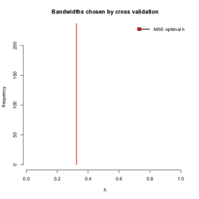
We simulate replications and use . We choose to be the largest local minimum of . In Figure 1 (left) we have plotted a histogram of the bandwidths chosen by our algorithm, together with the deterministic bandwidth from (5) which minimizes (and is not available in practice). We observe that concentrates around with Gaussian shape. To judge the performance of our procedure, we compare the achieved distances for , where is the bandwidth which minimizes on the current realization. In Figure 1 (right), we have visualized the results with a boxplot. We can see that performs quite well, the values of are comparable to those of .
 |
 |
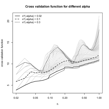
More satisfying results could be obtained by choosing dependent on the realization. For a fixed realization, it may occur due to nonasymptotic behavior that a single fixed does lead to cross validation functional (cf. (6)) which has no local minima. In practice it is therefore recommended to apply the procedure to different covering the whole interval and search for a suitable minimizer to obtain more stable bandwidth choices. In Figure 2 we have shown the curves obtained for different such that is ranging from to in steps of 0.01. From the definition of or it is obvious that one should look for a local minimum of with respect to and not for a global minimum (the latter would result in very small values of such as and therefore to an overfitting of the observations ). It can be seen in Figure 2 that for some no local minimum is available. The whole collection of functions, however, gives a well-founded indication which to choose, namely an close to which corresponds to the smallest local minimum of . Smaller with a reasonable shape of are preferred since then more observations in the direct neighbourhood of are used to estimate . This has lead to the choice and the resulting local minimum (from a practical point of view, one may also consider to choose the second local minimum where the situation seems to be more stable. This leads to similar results as above).
3.1.2 Estimation of
Writing and , we have and
We perform replications with . As before, we compare chosen by cross validation with which minimizes the integrated mean-quared error and . In Figure 3 (left) we plotted the bandwidths and as a vertical red line, in Figure 3 (right) one can see the boxplots corresponding to for . As before, concentrates around and the distances , are of comparable size.
 |
 |
3.1.3 Estimation of
Writing with , we have
To perform the simulations, we choose . Again, we use replications with . We compare chosen by cross validation with which minimizes the integrated mean-quared error and . In Figure 4 (left) we plotted the bandwidths and as a vertical red line, in Figure 4 (right) one can see the boxplots corresponding to for . Again, the results are satisfying in our opinion.
 |
 |
4 Local model selection: A contrast minimization approach
The approach presented in the following allows to choose locally for each in the estimator . This enables the procedure to take into account local smoothness changes of the function . The algorithm is based on a contrast minimization approach which was introduced by lepski2011 for a different model. In the following we use a slightly modified estimator for , namely
which corrects for the deviation of the kernel Riemannian sum from its integral .
The approach is based on a comparison of with the theoretical variance of . This leads to a procedure which does not need to estimate the bias of but only its variance and still finds a approximate minimizer of the corresponding mean squared error. As seen in Theorem 2.9, the asymptotic variance of is connected to the so-called long-run variance of ,
Let be an estimator of . In practice, the requirements on the quality of are not too strong, however we need that it has the same order of magnitude as . Large deviations from the true may lead to instable bandwidth choices. For theoretical derivations, we suppose:
Assumption 4.1 (Assumptions on ).
There exists some constant such that for each ,
-
•
is consistent such that for every , .
-
•
.
A possible choice for is given by
| (9) |
with some , and . We are now able to define the local bandwidth selection procedure as follows: Let and
Let be a geometrically decaying grid of bandwidths given by
| (10) |
where is some lower bound specified below. For some , define
| (11) |
Remark 4.2.
-
•
is approximately the variance of . It is multiplied by a log factor to account for local random deviations. As described in lepski2011 , the bandwidth (11) can be seen as the largest bandwidth where does not deviate significantly from .
-
•
To prove theoretical results, should not allow for too small bandwidths.
-
•
The condition is needed for the theoretical results. However, for many applications should be chosen smaller to avoid too conservative (i.e. too large) choices of .
We now provide the assumptions on the process under which the theoretical statements for the local bandwidth selection procedure holds.
Assumption 4.3 (Moment / Dependence assumptions).
Let . Let Assumption 2.1 hold for all . Define . Assume that for all ,
-
(i)
,
-
(ii)
.
Remark 4.4.
The assumptions stated above are mainly used to prove a Bernstein inequality which is a key ingredient to prove the consistency of contrast minimization methods. The geometric dependence decay is used to apply a Bernstein inequality from doukhanneumann2007 , while the moment conditions are necessary to allow for a large set of bandwidths by establishing a simple exponential inequality. The Bernstein inequality is formulated in terms of the process
which is a natural approximation of itself. The deviation can be controlled by using the property from Assumption 2.1.
Theorem 4.5 (Bernstein inequality for ).
The following theorem states that is bounded by an universal constant times up to an additional log-factor (cf. (4) for ).
Theorem 4.6.
Suppose further that such that for all , and is twice continuously differentiable around with .
Then there exists some universal constant and some constant only dependent on such that for , and large enough,
Remark 4.7.
The parameter is a tuning parameter of the procedure. However, from a theoretical point of view it does not depend on unknown quantities like but is a universal constant and therefore can be chosen based on training data before applying the procedure to real data. In practice, we obtained good results with .
4.1 Simulations
We discuss the behavior of if the underlying time series model is a tvAR(1) process given by (8) with i.i.d. and
-
[(a)]
-
1.
,
-
2.
In both situations we will estimate
by using replications of the time series with length . In the simulations, we use the Epanechnikov kernel and the set of bandwidths with and with (for (a)) and (for (b)). We estimate the long run variance by given in (9) with a simple ad-hoc choice of and .
A typical phenomenon arises if is chosen too small, i.e. allows for too small bandwidths: Then, tends to select the smallest possible bandwidth abruptly at random locations . The theoretical reason being that in such cases does not fulfill which is needed to discuss large deviations of in the Bernstein inequality. In practice, one may apply the selection procedure for all and for different , choosing the smallest where no abrupt outliers occur.
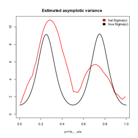
In Figure 5 (left) we depicted the typical behavior of (red) for the two scenarios (a),(b) for a single realization. Moreover, itself is drawn with a green line. The rough shape of is due to the stepwise form of . Generally speaking it can be seen that gets smaller if a too large bandwidth would introduce an unnecessary bias (see the peaks in (a) or the step in (b)). gets large if the variance of the procedure can be significantly reduced. In (b), this is the case on the boundaries where a nearly constant function has to be estimated and in the exact middle at where the target value 0 is estimated best by taking the mean over all observations. In (a) this is the case at points where has nearly linear shape (turning points). A typical drawback of the local selection procedure is that it may be more sensitive to strong local dependencies. In (b) one can see that around , is much smaller than the bandwidths chosen around it which is due to a strong peak of the process which is due to a violation of the asymptotic statements. In Figure 5 (right) the corresponding covariance estimator is drawn against the true long run variance . It can be seen that the method works quite satisfying even if is not estimated well; however it is important that the order of magnitudes coincide. Comparing (red) and (blue), where , it can be seen that in case (b), the local bandwidth selection may outperform the global bandwidth selection because of the significantly changing smoothness properties of .
| (a) | 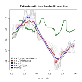 |
 |
|---|---|---|
| (b) | 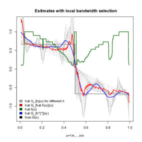 |
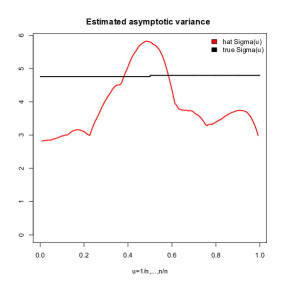 |
In the following we choose the weight function and compare the integrated distance for the local selector and the global optimal selector which is not known in practice. The results are summarized in Figure 6 via boxplots (right) and 0.05- and 0.95-quantile curves (left). It should be noted that even comparable results of with are worth to be emphasized since suffers from the typical higher variance of a data-driven selection procedure which is not the case for . In case (a), we see that the quantile curves of both selection procedures are comparable with a little bit higher variance around the peaks . The global optimal bandwidth clearly outperforms since has nearly smoothness properties over the whole time line.
In the case (b), it can be seen from the quantile curves that for near and , the local selector outperforms the global optimal selector since it is able to choose larger bandwidths there, reducing the variance of . For around , manages to mimic the step of the true function better than the global selector .
| (a) | 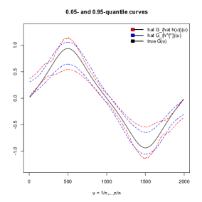 |
 |
|---|---|---|
| (b) | 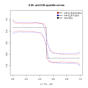 |
 |
5 Conclusion
In this paper, we have developed two methods for bandwidth selection for nonparametric moment estimators of locally stationary processes of some curve . We have derived theoretical results for their optimality with respect to mean-squared-error type distance measures and found with simulations that they work quite well in practice. The first method is based on a cross validation approach and allows for global bandwidth selection. A critical issue is to deal with the dependency of the observed time series which is controlled by some quantity . We have given theoretical and heuristical motivations how to choose this value to obtain a stable procedure. It should be emphasized that this choice is rather straightforward and data-dependent and therefore should not be considered as a tuning parameter. In a series of remarks, we have shown how to generalize our method to more general settings, for instance if is a composition of moment functions.
The second method is for local bandwidth selection, i.e. for each time point a different bandwidth is chosen. This allows for taking into account local smoothness properties of the unknown curve. The method needs an estimator of the asymptotic long-run variance and is dependent on a parameter . We have seen that the quality of does not influence the bandwidth selection procedure very much, while the choice of however is crucial to obtain meaningful results. In our theoretical results we have shown that is some universal constant which does not need to depend on the unknown quantities to be estimated. However, the conditions stated in theory may lead to too conservative estimates (i.e. the variance is reduced too strongly by introducing a large bias). In our simulations we have given ad hoc choices of which work fairly well, but in more specific applications it may be necessary to adjust further. We have seen in simulations that the local bandwidth selection procedure may outperform global bandwidth selection procedures. Finally, it should be noted that the presented local bandwidth selection procedure reduces the problem of choosing several tuning parameters separately (all the local bandwidths , ) to a proper choice of .
In practice, we propose to first use the cross validation method for a first guess of the global optimal bandwidth. Afterwards one may apply the local selection procedure, using (or the estimator of based on , respectively) to calibrate .
One may try to improve the theory for the presented methods, allowing for more general structures of and its estimators or investigating with moments of two sided functions. These questions are left to further research.
6 Appendix
During the proofs, is a generic constant which may depend on
-
•
(from ),
- •
-
•
(the kernel).
Its value may change from line to line. We define
and .
Proof of Theorem 2.7.
(i) By Lemma 6.6(ii), we have in each component that
Since is twice differentiable, the same holds for each component of by using the chain rule. We conclude that
and
| (13) | |||||
Due to Lipschitz continuity and symmetry of , the first two terms in (13) are . The third term in (13) is .
Due to Assumption 2.6, it can be seen with Hoelder’s inequality that
The dominated convergence theorem yields that the last term in (13) is , giving the final result.
(ii) By Lemma 6.6(ii), we have in each component that
We furthermore have
| (14) |
Similar as in (i), we obtain
| (15) |
By Lemma 6.7, we have
| (16) | |||||
∎
6.1 Proof of Theorem 3.1
Proof of Theorem 3.1.
We use the proof techniques from richterdahlhaus2018aos . Choosing , we find that is uniquely minimized by .
Assumptions 3.1, 3.3, 3.4 and 3.7 easily follow from the assumptions stated at the beginning (weight function …, set of bandwidths , twice continuously diff, conditions on , twice cont. …). It can be easily seen that Assumption 3.7(3) therein is only needed in the version we ask for on .
The only condition which is not fulfilled is Assumption 3.3(4) therein, which asks
to be an uncorrelated sequence. We now follow the main steps of the proof of Theorem 3.6 in richterdahlhaus2018aos and emphasize the steps where the condition of uncorrelatedness has to be circumvented.
By (18) in richterdahlhaus2018aos , we have uniformly in ,
| (17) | |||||
Using the same arguments as in richterdahlhaus2018aos , equation (26) therein, we have
| (18) |
Define
Then we have
where with ,
Note that is Lipschitz-continuous in the sense that
with some polynomial in . This allows us to use chaining arguments to prove uniform convergences in . In the following we use the decomposition
where with and ,
Since for all , , it is easy to see by a chaining argument that a.s.
Note that
and for with ,
By Lemma 6.2, we have , thus with some constant ,
Therefore we obtain if .
Using Lemma 8.1(ii) from the Supplementary material of richterdahlhaus2018aos , we have with some constants ,
which shows that .
Finally, by the same Lemma we obtain for all with some constant :
showing with a chaining argument that a.s. In total, we have seen that
and thus with (17),
| (19) |
We now analyze the difference
Following the proof of Lemma 3.16 in richterdahlhaus2018aos , we show
| (20) |
Define . Following the proof of Lemma 2.5 in richterdahlhaus2018aos ((41) and the discussion of , , , therein), we obtain that
fulfills a.s. To use the argument for therein to obtain (20), we have to verify that
| (21) |
We now cannot argue with the uncorrelatedness of . Instead we use a direct calculation of : It holds that with some (cf. also (39)), thus
which shows (21) if .
Using (20), (19) and (18), the result now follows along the same lines as the proof of Theorem 3.6 in richterdahlhaus2018aos . ∎
6.2 Proof of Theorem 4.6
Proof of Theorem 4.6.
Define . Since , for large enough it holds that
Furthermore, with some constant only depending on , and the corresponding Lipschitz constants of :
Since is twice continuously differentiable,
We obtain
and thus for small enough, . Define
By Proposition 6.1, we have
| (22) | |||||
For the second summand in (22) we find, for large enough, the upper bound
which together with (22) gives the result. ∎
Proposition 6.1.
Proof of Proposition 6.1.
We follow the proof strategy of lepski2011 . During the proof, we use for a constant only dependent on . Put
Define
Then
| (23) |
Discussion of the first summand in (23): It holds that
| (24) | |||||
By Lemma 6.6 and Lemma 6.7 and since for large enough, we have
| (25) | |||||
By definition of and monotonicity of ,
| (26) |
We now discuss . It holds that
for large enough due to Assumption 4.1. We therefore have
| (27) |
Using (26) and (27), we obtain
| (28) |
By definition of , we have
| (29) |
Inserting (25), (28) and (29) into (24), we obtain
| (30) |
Discussion of the second summand in (23): Let . By definition of and by monotonicity of , , we obtain for :
| (31) |
Decompose
Let
and define
We have
We conclude with the Cauchy-Schwarz inequality, (31) and Assumption 4.1:
With Lemma 6.6, we can replace with with error due to
Similarly, the set has the property
allowing to replace by in with replacement error . Together with , we have shown that
fulfills
| (32) | |||||
Put and . We now discuss the summands in (32). It holds that
| (33) | |||||
Discussion of the first summand in (33). Put and . Then, with Lemma 6.5,
By Lemma 6.7(ii), is fulfilled if
i.e. if for large enough (which is fulfilled due to ). We obtain that for , with :
| (34) |
Discussion of the second summand in (33). We have by Lemma 4.5 that
We have with :
Thus
| (35) | |||||
We now discuss the first two summands in (35). We have
and, with some constant only depending on ,
Here,
| (36) |
We conclude that (36) is if for large enough (which is fulfilled due to ). Clearly, (36) is . Summarizing these results into (35), we obtain for all that
| (37) |
with some constant .
Lemma 6.2.
Assume that . Suppose that Assumption 4.3 holds. Put . Then there exist constants only depending on such that for :
Proof of Lemma 6.2:.
(i) It holds that
Since , we obtain with some only depending on .
(ii) Define . By a series expansion of , we have
If , we have
This shows .
In the case , we have
This shows . The result is obtained with . ∎
Lemma 6.3 (Exponential inequality).
Assume that is some measurable function, and . Suppose that Assumption 4.3 holds. Define
Put . Then there exist constants only depending on such that
-
(i)
-
(ii)
Proof of Lemma 6.3.
(i) Let . By Hoelder’s inequality, we have with some constant only dependent on :
| (39) | |||||
Let . Obviously, . We have shown that the dependence measure fulfills and is absolutely summable.
By Theorem 2.1 from rio2009 for (and for directly by calculating the variance of the following term), we have
(ii) Define . By Stirling’s formula, we have for all :
By Markov’s inequality, we have for :
In the case , we have
Note that and , thus
Define . Since , it holds that . Thus
In the case , we have
thus . So the result is obtained with and . ∎
Lemma 6.4 (Bernstein inequality).
Proof.
(i) Step 1: Truncation. Define , where , ,
We have
| (41) | |||||
By Lemma 6.2, we have
Inserting this into (41) and using Lemma 6.2 to bound , we obtain.
| (42) |
With (42) and Markov’s inequality, we obtain
| (43) | |||||
Step 2: Applying a Bernstein inequality from doukhanneumann2007 . Note that by Assumption 4.3 and (39), we have with some constant only dependent on :
i.e.
| (44) |
with , only depending on .
For , it holds that
We have
By Lemma 6.2, . We obtain with (44) and Lipschitz continuity of that
Furthermore,
Using Theorem 1 in doukhanneumann2007 (with , therein) yields
where and with ,
(we use instead of which is possible due to a change in the upper bound in their equation (43)). Here, we have with (42) and that
By assumption, we conclude that for large enough. ∎
Proof of Theorem 4.5.
Furthermore, we obtain a Bernstein inequality for the difference for two different bandwidths :
Lemma 6.5 (Bernstein inequality for ).
Proof of Theorem 4.5.
Lemma 6.6 (Stationary approximation).
Let . Then with some constant ,
-
(i)
.
-
(ii)
uniformly in , .
Proof of Lemma 6.6.
(i) By Hoelder’s inequality,
| (45) | |||||
Put . Then
If , then summation is only done over , thus . Since , we obtain the result.
If , then and , we obtain the result.
Lemma 6.7 (Calculation of Variance).
Assume that
fulfills . For with , it holds that (i)
and for (with fixed ), there exist constants such that (ii)
where , .
Proof of Lemma 6.7.
(i) Put . With some constant only dependent on , we have by (44),
and thus
| (46) | |||||
Since , we have with some constant only dependent on that
| (47) |
thus
| (48) |
Abbreviate . Then
| (49) | |||||
can be replaced by due to Lipschitz-continuity (Lipschitz constant ) of with replacement error
due to (44) with some only depending on . After the replacement, (49) reads
Since is Lipschitz continuous, this can be replaced by with replacement error .
(ii) First note that we have with :
Let . Then
by assumption, and
Since is a continuous function, we conclude that , and thus
fulfills
We conclude that
The rest of the proof is the same as in (i).
∎
References
- [1] Cristina Amado and Timo Teräsvirta. Modelling volatility by variance decomposition. J. Econometrics, 175(2):142–153, 2013.
- [2] Cristina Amado and Timo Teräsvirta. Specification and testing of multiplicative time-varying GARCH models with applications. Econometric Rev., 36(4):421–446, 2017.
- [3] Ouerdia Arkoun. Sequential adaptive estimators in nonparametric autoregressive models. Sequential Anal., 30(2):229–247, 2011.
- [4] Ouerdia Arkoun and Serguei Pergamenchtchikov. Sequential robust estimation for nonparametric autoregressive models. Sequential Anal., 35(4):489–515, 2016.
- [5] R. Dahlhaus. Fitting time series models to nonstationary processes. Ann. Statist., 25(1):1–37, 1997.
- [6] R. Dahlhaus, S. Richter, and W. B. Wu. Towards a general theory for non-linear locally stationary processes. Bernoulli, to appear, ArXiv e-prints: 1704.02860, 1 2019.
- [7] Rainer Dahlhaus and Suhasini Subba Rao. Statistical inference for time-varying ARCH processes. Ann. Statist., 34(3):1075–1114, 2006.
- [8] Paul Doukhan and Michael H. Neumann. Probability and moment inequalities for sums of weakly dependent random variables, with applications. Stochastic Process. Appl., 117(7):878–903, 2007.
- [9] Christophe Giraud, François Roueff, and Andres Sanchez-Perez. Aggregation of predictors for nonstationary sub-linear processes and online adaptive forecasting of time varying autoregressive processes. Ann. Statist., 43(6):2412–2450, 2015.
- [10] Carsten Jentsch, Anne Leucht, Marco Meyer, and Carina Beering. Empirical characteristic functions-based estimation and distance correlation for locally stationary processes. Working Paper Series 16-15, Mannheim, 2016. urn:nbn:de:bsz:180-madoc-414388.
- [11] Bonsoo Koo and Oliver Linton. Estimation of semiparametric locally stationary diffusion models. J. Econometrics, 170(1):210–233, 2012.
- [12] O. V. Lepski, E. Mammen, and V. G. Spokoiny. Optimal spatial adaptation to inhomogeneous smoothness: an approach based on kernel estimates with variable bandwidth selectors. Ann. Statist., 25(3):929–947, 1997.
- [13] Stéphane Mallat, George Papanicolaou, and Zhifeng Zhang. Adaptive covariance estimation of locally stationary processes. Ann. Statist., 26(1):1–47, 1998.
- [14] M. B. Priestley. Evolutionary spectra and non-stationary processes.(With discussion). J. Roy. Statist. Soc. Ser. B, 27:204–237, 1965.
- [15] M. B. Priestley. Nonlinear and nonstationary time series analysis. Academic Press, Inc. [Harcourt Brace Jovanovich, Publishers], London, 1988.
- [16] S. Richter and R. Dahlhaus. Cross validation for locally stationary processes. Annals of Statistics, to appear, ArXiv e-prints: 1705.10046, 01 2019.
- [17] Emmanuel Rio. Moment inequalities for sums of dependent random variables under projective conditions. J. Theoret. Probab., 22(1):146–163, 2009.
- [18] François Roueff, Rainer von Sachs, and Laure Sansonnet. Locally stationary Hawkes processes. Stochastic Process. Appl., 126(6):1710–1743, 2016.
- [19] Suhasini Subba Rao. On some nonstationary, nonlinear random processes and their stationary approximations. Adv. in Appl. Probab., 38(4):1155–1172, 2006.
- [20] Michael Vogt. Nonparametric regression for locally stationary time series. Ann. Statist., 40(5):2601–2633, 2012.
- [21] Wei Biao Wu. Nonlinear system theory: another look at dependence. Proc. Natl. Acad. Sci. USA, 102(40):14150–14154, 2005.
- [22] Wei Biao Wu and Zhou Zhou. Gaussian approximations for non-stationary multiple time series. Statist. Sinica, 21(3):1397–1413, 2011.