Spin squeezing by one-photon-two-atom excitations processes in atomic ensembles

Abstract

It has been shown elsewhere that two spatially separated atoms can jointly absorb one photon, whose frequency is equal to the sum of the transition frequencies of the two atoms. We describe this process in the presence of an ensemble of many two-level atoms, and show that it can be used to generate spin squeezing and entanglement. This resonant collective process allows to create a sizeable squeezing already at the single-photon limit. It represents a novel way for generating many-body spin-spin interactions, yielding a two-axis twisting-like interaction among the spins, which is very efficient for the generation of spin squeezing. We perform explicit calculations for ensembles of magnetic molecules coupled to a superconducting coplanar cavities. This system represents an attractive on-chip architecture for the realization of improved sensing.

I Introduction

Recently, it has been shown how a large number of nonlinear optics processes can be realized with individual two-level atoms coupled to one or more resonator modes in the ultrastrong coupling regime (USC)Kockum et al. (2017), where the coupling strength starts to become comparable to the resonance frequencies of the bare system components. In this regime, counter-rotating terms in the light-matter interaction Hamiltonian start to play a role and enable novel higher-order processes Kockum et al. (2019); Forn-Díaz et al. (2019). These vacuum-boosted nonlinear-optics implementations, in contrast to conventional realizations of various multi-wave mixing processes in nonlinear optics, can reach perfect efficiency, need only a minimal number of photons, and require only two atomic levels.

Many of these processes can be described in terms of higher-order perturbation theory, in which the system passes from an initial state $|i\rangle$ to the final state $|f\rangle$ (with the same energy), via a number of virtual transitions to intermediate states. When the light–matter coupling strength increases, the vacuum fluctuations of the electromagnetic field become able to induce efficiently such virtual transitions, replacing the role of the intense applied fields in conventional nonlinear optics. In this way, higher-order processes involving counter-rotating terms can create an effective coupling between two states of the system ($|i\rangle$ and $|f\rangle$) which can have different number of excitations. The strength of the resulting effective coupling scales approximately as $g_{\rm eff}\sim g(g/\omega)^{n}$, where $g$ is the light-matter coupling strength, $\omega$ describes a bare resonance frequency of the light or matter component, and $n$ is the number of involved virtual transitions. However, the required light-matter coupling strength to observe these deterministic nonlinear optics effects with the minimum amount of photons, can only be reached, at least presently, only with superconducting artificial atoms. Recently, simulations of these nonlinear optics effects with strong-coupling systems (with $g/\omega\ll 1$) dressed by classical drives have been proposed Ballester et al. (2012); Pedernales et al. (2015); Braumüller et al. (2017); Dingshun et al. (2018); Muñoz et al. (2019).

Here, we propose a different route, already widely explored to observe linear optical processes in the USC regime: the light–matter coupling strength can be enhanced by increasing the number $N$ of emitters interacting with the resonator. The resulting collective coupling strength scales as $g\sqrt{N}$. In this way the USC regime can be reached in a wider range of systems (see, e.g., Schwartz et al. (2011); Kéna-Cohen et al. (2013); Gubbin et al. (2014); Mazzeo et al. (2014); Gambino et al. (2014); Anappara et al. (2009); Genco et al. (2018); Günter et al. (2009); Todorov et al. (2010); Scalari et al. (2012); Maissen et al. (2014); Zhang et al. (2016); Li et al. (2018)).

One of the most interesting nonlinear optical effects predicted in the USC regime consists of the simultaneously excitation of two or more spatially separated atoms by a single photon Garziano et al. (2016); Zhao et al. (2017); Wang et al. (2017). This process is reversible, so that the atoms can return to a lower-energy state by collectively emitting one photon. This is a two-atom resonant process occurring when the atom transition is half of the cavity frequency. Here, we generalize this process to many two-level atoms which can be described as an ensemble of $N$ pseudo-spins.. This opens the way to investigate cases in which several photons can excite different atomic pairs, producing an effective, controllable interaction among spins. As we will show, the simultaneous excitation of spin pairs in a large ensemble, can give rise to multi-atom entanglement and to strong spin squeezing, which could be useful for application in quantum technologies.

Quantum sensors beat the shot-noise limit of precision by using entangled states. Pseudo spin-$1/2$ ensembles, serving as probes for measuring a magnetic field, represent a paradigmatic example Tóth and Apellaniz (2014). If they are prepared in a convenient squeezed-entangled state, the minimized quadrature reduces the precession angle uncertainty and, thus, the error in the field estimation Ma et al. (2011). The Heisenberg principle imposes the ultimate scaling error as $1/N$, with $N$ the number of spins. Therefore, preparing a macroscopic spin state in a highly squeezed state is a key resource for quantum metrology.

Squeezed states in atomic ensembles are prepared by inducing interactions among the spins. Different schemes, including atom-atom interactions in traps, feedback and projective measurements have shown up to -18 dB quadrature reduction Riedel et al. (2010); Ian et al. (2010); Wasilewski et al. (2010); Muessel et al. (2014); Schleier-Smith et al. (2010); Bohnet et al. (2014); Vasilakis et al. (2015); Hosten et al. (2016a).

An interesting alternative is the deterministic production within one-axis twisting interactions generated inside a cavity Hosten et al. (2016b); Norcia et al. (2018). So far, the reported results are limited to -8 dB. Thus, it is desirable to find improved but deterministic protocols, as the preparation of initial coherent states superpositions Lewis-Swan et al. (2018).

Another alternative involves considering two-axis twisting Hamiltonians that are known to be optimal for generating squeezing Opatrný (2015); Liu et al. (2011). However, it remains to show their advantage in presence of noise and decoherence Borregaard et al. (2017). It has been shown that collective decoherence can be suppressed via continuous dynamical decoupling Chaudhry and Gong (2012). This approach can make spin squeezing more robust to noise and closer to the Heisenberg limit (optimal squeezing, scaling a $\xi^{2}\sim 1/N$).

In this work we show that the one-photon-two-atom excitations process can determine approximate two-axis twisting interactions in spin ensembles coupled to a cavity mode, which are known to generate optimally squeezed states.

Our protocol is different from previous approaches in several ways. Although the light-matter system is in the dispersive regime, it is a resonant mechanism involving real photons. This is complementary to the case where the field can be integrated out, so that the spin-spin interactions are mediated by virtual photons Agarwal et al. (1997); Sørensen and Mølmer (2002); Borregaard et al. (2017). The approach proposed here is a third-order nonlinear optical process boosted by virtual photons Kockum et al. (2017). Therefore, for obtaining a significant rate for the excitation of atom pairs, even for weak input fields, the light-atoms coupling rate should reach a significant fraction of the atomic transition frequency.

However, in this work, the relevant coupling strength is not the single-spin coupling, $g$, but the effective collective interaction between the $N$ spins and the single-cavity mode, which yields the scaling $\sim g^{3}N$. This widely broadens the number of platforms where this process could be implemented.

Moreover, it is also required that the atomic or molecular potential does not display inversion symmetry. In this case, the system can be described by an extended Dicke model, with atoms displaying both longitudinal and transverse coupling with the cavity mode (see, e.g., Ref.s Garziano et al. (2015, 2016); Lambert et al. (2018)).

Finally, real photons must be injected inside the cavity. The drive could be even a coherent resonant field. Unexpectedly, we find that even a single cavity photon is able to generate a significant amount of squeezing. A final advantage of using resonant real photons is that the interaction can be controlled by acting either on the driving or on the atoms-cavity detuning.

Our results could be implemented using several kinds of qubits as, e.g., cold atoms, chiral molecules or superconducting flux qubits. One interesting architecture consists of hybrid spin-superconductor systems et al. (2013a), where the spins can be NV-centers Schuster et al. (2010); Kubo et al. (2010); Wu et al. (2010); Amsüss et al. (2011); et al. (2013b, c) or more general spins Jenkins et al. (2013, 2016) that are coupled to a superconducting microwave resonator.

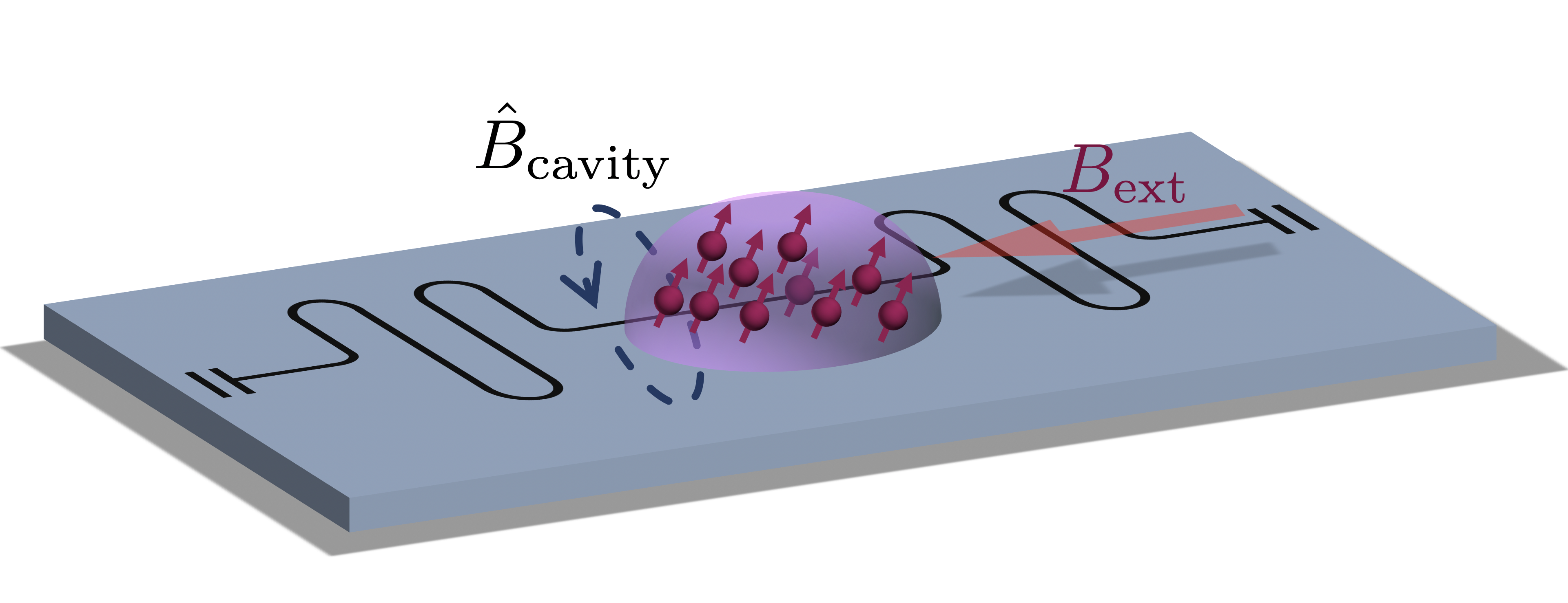
Figure 1: Sketch for the proposed architecture. An ensemble of magnetic molecules (red in the figure) are deposited on top of a superconducting coplanar waveguide resonator. The spin-cavity coupling is mediated by the magnetic field generated by the stationary currents in the circuit, denoted in the figure as $\hat{B}_{\rm cavity}$. The spins transition frequency can be tuned by means of external control fields, $\hat{B}_{\rm ext}$.

II Resonant excitation of atomic pairs: effective Hamiltonian and squeezing parameter

We consider an ensemble of $N$ identical two-level systems equally coupled to a single-mode cavity. The Hamiltonian can be written as:

$$\hat{H}=\Delta\hat{J}_{z}+\epsilon\hat{J}_{x}+\omega_{\rm c}\,\hat{a}^{\dagger}\hat{a}+2g(\hat{a}+\hat{a}^{\dagger})\hat{J}_{x}\,,$$ (1)

where $\hat{a}$ and $\hat{a}^{\dagger}$ are the usual operators for cavity photons, while $2\hat{J}_{\alpha}=\sum_{i}\hat{\sigma}_{\alpha}^{i}$ ($\alpha=x,y,z$) are the collective angular momentum operators. As a consequence of the latter expression, lowering and raising spin operators are defined as $\hat{J}_{\pm}=\sum_{i}\hat{\sigma}^{i}_{\pm}$. Parity symmetry breaking is described by the second term in Eq. (1). For $\epsilon=0$ the celebrated Dicke model is recovered Garraway (2011); Shammah et al. (2017, 2018); Kirton et al. (2019). When $\epsilon\neq 0$, $\hat{H}$ can couple states differing by an odd number of excitations. For example, an avoided level crossing, originating from the coupling of the states $\hat{a}^{\dagger}|0,j,-j\rangle\leftrightarrow\hat{J}_{+}^{2}|0,j,-j\rangle$, is expected when the resonance frequency of the cavity $\omega_{c}\simeq 2\omega_{q}=\sqrt{\Delta^{2}+\epsilon^{2}}$. We label the states as $|n,j,m\rangle$, where the quantum number $n$ describes the Fock states of the cavity, and $j=N/2$ is the total angular momentum and $m=-j+N_{\rm exc}$ is the $\hat{J}_{z}$ eigenstate, where $N_{\rm exc}$ describes the number of excited atoms. Such a coupling has been described for the two qubit case ($N=2$) only in Garziano et al. (2016). Figure 2 confirms that it also occurs for any $N\geq 2$. The analysis of those processes non-conserving the number of excitations can be simplified, deriving an effective Hamiltonian by using perturbation theory Shao et al. (2017). For frequencies close to the resonance condition $\omega_{c}\simeq 2\omega_{q}$, from Eq. (1), as shown in Appendix A, the following effective interaction Hamiltonian can be obtained:

$$\hat{H}_{\rm eff}=g_{\rm eff}\left(\hat{a}\hat{J}_{+}^{2}+\hat{a}^{{\dagger}}\hat{J}_{-}^{2}\right)\,,$$ (2)

where

$$g_{\rm eff}=-\frac{4g^{3}\cos^{2}\theta\sin\theta}{3\omega^{2}_{q}}\,,$$ (3)

with $\sin\theta=\epsilon/\sqrt{\Delta^{2}+\epsilon^{2}}$. This procedure also gives rise to a renormalization of the atomic frequencies, which can be reabsorbed into $\omega_{q}$.

The effective Hamiltonian Eq. (2) yields a series of nonzero transition matrix elements $\langle n-1,j,m+2|\hat{H}_{\rm eff}|n,j,m\rangle$, determining a ladder of avoided level crossings at $\omega_{c}=2\omega_{q}$, with energy splittings which are twice these matrix elements. The lowest energy splitting is

$$\Delta E=2g_{\rm eff}\sqrt{2N(N-1)}\,.$$ (4)

It is worth noticing that, for large $N$, this splitting scales as $\sim\!g^{3}N$. The comparison between $\Delta E/2$ and the corresponding half-splitting energy obtained from the exact numerical diagonalization of the Hamiltonian in Eq. (1) is shown in the inset in Fig. 2. We note the very good agreement. Figure 2 displays the lowest excited energy levels of the effective Hamiltonian (the ground state energy is zero) as a function of $\omega_{c}/\omega_{q}$, obtained for $N=20$ qubits. Avoided level crossings are clearly visible at $\omega_{c}\simeq 2\omega_{q}$. In Appendix B, we also compare the higher energy avoided level crossings obtained by using the full Eq. (1) and the effective Eq. (2) models. The results still show a quite good agreement for $\omega_{c}\simeq 2\omega_{q}$.

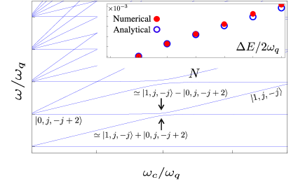
Figure 2: Lowest energy levels of the system Hamiltonian obtained for $N=20$ qubits as function of the ratio between the cavity frequency $\omega_{c}$ and that of identical qubits $\omega_{q}$. We used $g=2.5\times 10^{-4}\,\omega_{q}$ and $\theta=\pi/6$. The inset compares the analytical (blue dots) and numerical (red dots) results for the effective coupling between the states $|0,j,-j+2\rangle$ and $|1,j,-j\rangle$ versus the number of qubits.

To characterize the squeezing we use the spin-squeezing parameter $\xi^{2}$, proposed by Wineland et al. Ma et al. (2011); Wineland et al. (1992, 1994),

$$\xi^{2}=N\frac{\langle(\hat{\bf J}\cdot{\bf n}_{\perp})^{2}\rangle-\langle\hat{\bf J}\cdot{\bf n}_{\perp}\rangle^{2}}{\langle\hat{\bf J}\rangle^{2}}\,,$$ (5)

where the unit vector ${\bf n}_{\perp}$ is chosen to minimize the numerator. This is the ratio between the fluctuations of a general state versus the coherent spin state (CSS), for the determination of the resonance frequency in Ramsey spectroscopy. The CSS here acts as a noise-reference state. For $\xi<1$ a gain in interferometric precision is possible compared to using a coherent spin state Ma et al. (2011); Wineland et al. (1994).

II.1 Single photon squeezing

The simplest and, at the same time, weirdest illustration of the role of real cavity photons in spin squeezing generation can be obtained by looking at the squeezing generated by a single photon. Let us consider as initial state a superposition of zero and one photon, with all the atoms in their ground state: $|\psi(0)\rangle=\cos\varphi|0,j,-j\rangle+\sin\varphi|1,j,-j\rangle$. Using the effective Hamiltonian in Eq. (2) and neglecting the losses, the time evolution can be analytically calculated:

$$|\psi(t)\rangle = \cos\varphi|0,j,-j\rangle+\sin\varphi\cos(g_{\rm eff}t)|1,j,-j\rangle$$ (6)

$$- i\sin\varphi\sin(g_{\rm eff}t)|0,j,-j+2\rangle\,,$$

from which the spin squeezing parameter in Eq. (5) can be obtained. We chose ${\bf n}_{\perp}=(\cos\phi,\sin\phi,0)$ (orthogonal to the $z$ axis). In Fig. 3(a) we plot the time evolution of $\xi^{2}$. We also show the mean photon number

$$\langle\hat{a}^{{\dagger}}\hat{a}\rangle=\sin^{2}\!\varphi\,\cos^{2}(g_{\rm eff}t)\,,$$ (7)

and the mean number of excited atoms

$$N_{\rm exc}=j+\langle\hat{J}_{z}\rangle=2\sin^{2}\varphi\,\sin^{2}(g_{\rm eff}t)\,.$$ (8)

We considered a system of $N=20$ spins with parameters $g=0.115\,\omega_{q}$, $\theta=\pi/6$ (i.e., $g_{\rm eff}=0.01$), and $\varphi=0.45\pi$. We also used the phase $\phi=\pi/4$, providing the maximum squeezing (corresponding to the minimum value of $\xi^{2}$). When the cavity excitation is completely transferred to the ensemble of two-level systems, the squeezing reaches its maximum. This is because the system is in a quantum superposition of the states $|j,-j\rangle$ and $|j,-j+2\rangle$. They are the two first components of an even superposition of coherent states, i.e. an entangled cat state. Let us emphasize the maximum amount of quantum-noise reduction obtained, $\xi^{2}\simeq 0.55$, already with a single photon. Very similar results can be obtained using the full original Hamiltonian Eq. (1), as reported in Appendix B.

Notice, that the considered coupling strength $g$ between the resonator and each qubit can be realized experimentally with circuit-QED systems in the USC regime (see, e.g., Niemczyk et al. (2010). However, since the effective coupling scales linearly with $N$, increasing the number of superconducting qubits, even lower individual coupling strength can become sufficient. Notice that, the coherent coupling of superconducting resonators with very large ensembles of flux qubits have been demonstrated Kakuyanagi et al. (2016). Moreover, these systems can display decay rates much lower than the resulting effective coupling $\sim g_{\rm eff}{N}$. When the loss rates are equal or larger than five times $\sim g_{\rm eff}{N}$, they do not affect the dynamics shown in Fig. 3(a).

II.2 Dissipation and drivings beyond one-photon

We now move to the scenario where both the spins and the cavity are affected by dissipation. Assuming that each atom has a $\gamma$ decay channel, and applying the typical second-order Born and Markov approximations, we end up with the master equation for the density matrix of the cavity plus spins system [see, e.g., Gelhausen et al. (2017) and Appendix C]:

$$\dot{\hat{\varrho}}=-i[\hat{H},\hat{\varrho}]+\kappa{\mathcal{D}}[\hat{a}]+\frac{\gamma}{N}{\mathcal{D}}[\hat{J}_{-}]\,,$$ (9)

where ${\mathcal{D}}[\hat{O}]=\hat{O}\hat{\varrho}\hat{O}^{\dagger}-1/2\{\hat{O}^{\dagger}\hat{O},\hat{\varrho}\}$ are the dissipators in Lindblad form, and $\kappa$ and $\gamma$ are the loss rates for the cavity and the spins, respectively. Also, we discuss other kinds of drivings beyond the single-photon example of the preceding section.

Assuming that the system starts in its ground state, we first consider a resonant optical pulse feeding the cavity, including an additional time dependent Hamiltonian term $\hat{V}_{d}={\cal F}(t)(\hat{a}+\hat{a}^{\dagger})$, where ${\cal F}={\cal A}\,{\cal G}(t)\cos{(\omega_{\rm d}\,t)}$, with ${\cal G}(t)$ being a normalized Gaussian function. We consider pulses with their central frequency resonant with the cavity ($\omega_{\rm d}=\omega_{\rm c}$). Figure 3(b) displays the system dynamics after the pulse arrival, for a system consisting of a cavity mode and $N=10$ spins. The parameters used are $g=0.115\,\omega_{q}$, $\gamma=10^{-4}\omega_{q}$, $\kappa=\gamma/2$, ${\cal A}/\omega_{q}=3\pi/4$ and $\theta=\pi/6$. The Fig. 3(b) shows that the mean photon number $\langle\hat{a}^{{\dagger}}\hat{a}\rangle$, as expected, is anticorrelated to the mean collective spin excitation $j+\langle\hat{J}_{z}\rangle$. Here, the even spin states superposition involves higher spin states of the type $|j-j+2n\rangle$, which allows to generate a higher degree of spin squeezing. Notice that the obtained maximum spin squeezing (corresponding to the lowest value of the spin parameter $\xi^{2}$) is quite high, despite the cavity being fed with a weak coherent pulse producing a peak mean intracavity photon number slightly less than one.

We also investigate the case of weak continuous driving: ${\cal F}={\cal A}\,\cos{(\omega_{\rm d}\,t)}$ with ${\cal A}=2.5\;\gamma$. The other parameters used are, $g=0.115\,\omega_{q}$, $\gamma=10^{-3}\omega_{q}$ and $\kappa=\gamma$. In Fig. 3(c) we see that squeezing starts to build up when the spin population grows, as expected. In this case, because of the continuous character of the driving, both the cavity and the spins populate to reach a stationary value. The squeezing achieved in this full quantum simulation is quite low, owing to the losses and the low-excitation amplitude.

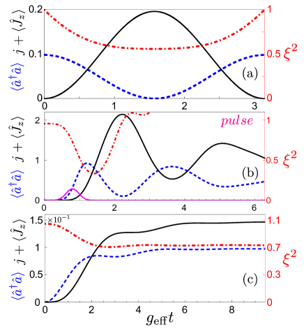
Figure 3: System dynamics for $\omega_{c}=2\omega_{q}$, (a) single-photon dynamics, (b) subject to a $\pi$-pulse (magenta solid curve) drive of the cavity mode and (c) under continuous-wave drive of the cavity mode. The blue dashed curve describes the mean photon number $\langle\hat{a}^{{\dagger}}\hat{a}\rangle$, while the black solid curve describes the mean collective spin excitation $j+\langle\hat{J}_{z}\rangle$. The squeezing parameter $\xi^{2}$ is also plotted as a red dot-dashed curve with values given on the $y$ axis on the right. All numerical parameters are given in the text.

II.3 Macroscopic spin ensemble

The full quantum numerical simulations are limited to few tens of qubits. However, for most practical purposes $N\gg 1$ is needed. When $N$ is sufficiently large, the collective spin operators can be replaced by a bosonic mode ($\hat{J}_{+}\to\sqrt{N}\,\hat{b}$), so that the squeezing parameter defined in Eq. (5) tends to the bosonic squeezing measure Ma et al. (2011); Wang and Sanders (2003),

$$\xi_{N\to\infty}^{2}=1+2(\langle\hat{b}^{\dagger}\hat{b}\rangle-|\langle\hat{b}^{2}\rangle|)\,.$$ (10)

In this limit, the effective Hamiltonian [Cf. Eq. (2)] becomes

$$\hat{H}_{\rm eff}=g_{\rm eff}N(\hat{a}{\hat{b}}^{\dagger 2}+\hat{a}^{\dagger}{\hat{b}}^{2})\,,$$ (11)

while the Lindbladians are replaced consistently:  $\frac{1}{N}{\mathcal{D}}[\hat{J}_{-}]\to{\mathcal{D}}[\hat{b}]$ [see Eq. (9)]. The Hamiltonian in Eq. (11), resulting from the bosonization of the effective Hamiltonian in Eq. (2), corresponds to the model Hamiltonian used to describe, in quantum optics, degenerate parametric processes, like second-harmonic generation and parametric down-conversion Mandel and Wolf (1995); Roy and Devoret (2016). Specifically, the term $\hat{a}{\hat{b}}^{\dagger 2}$ can describe the fission of a photon of a mode at frequency $\omega_{a}$ into a photon pair at frequency $\omega_{b}$ such that $\omega_{a}=2\omega_{b}$; while the term $\hat{a}^{\dagger}{\hat{b}}^{2}$ describes the opposite process, where two photons at frequency $\omega_{b}$ converts into a photon of the mode at frequency $\omega_{a}=2\omega_{b}$. Notice that the Hamiltonian in Eq. (11) also applies to the description of parametric processes in completely different systems (see, e.g., Macrì et al. (2018)).

We observe that the resulting coupling in Eq. (11) scales as $g^{3}N$. Such bosonic approximation is expected to work fine in the limit $g\to 0$ and $N\to\infty$, such that $g^{3}N\to$ constant. However, we point out that this approximation can work well even in the more physical case of a finite number of atoms, when the number of excitations in the system are significantly smaller than the number $N$ of atoms in the ensemble. Notice that, such limit is different from the usually considered thermodynamic limit of the Dicke model (see, e.g. Emary and Brandes (2003)), where $g\sqrt{N}\to$ constant is assumed. If the latter would have been assumed, the resulting coupling strength $g_{\rm eff}N$ in Eq. (11) would go to zero. This is not a surprise, since it is known that in the limit $g\to 0$ and $N\to\infty$, and $g\sqrt{N}\to$ constant, optical nonlinearities in the Dicke model disappear.

We also observe that the Dicke model in the dispersive regime gives rise to energy shifts of both the atomic and cavity resonances scaling as $g^{2}N$, which we limit to take into account phenomenologically, just adjusting the bare energy levels. Hence, increasing the number of atoms, while keeping constant the resulting coupling strength $g_{\rm eff}N$, determines relevant energy shifts which have to be taken into account.

In order to maximize squeezing, a strong driving is required. In this case, a direct simulation, using the full quantum models in Eq. (1), Eq. (2), or also in Eq. (11) becomes not feasible. Hence, we start from the dynamics induced by the Hamiltonian in Eq. (11) and apply the mean-field approximation in order to describe the cavity-spins dynamics Roy and Devoret (2016).

In experiments, it is possible to freeze the squeezed state at the time when the maximum squeezing is reached, by detuning the spins transition frequency. Then, the squeezing is preserved for a time determined by the spins decay rate $\gamma$. In order to better analyze the squeezing dynamics we derived the equation of motion for the squeezing parameter, in the mean-field approximation

$$\frac{d\xi^{2}}{dt}=-\big{(}i4g_{\rm eff}N\langle\hat{a}\rangle+\gamma\big{)}\xi^{2}+\gamma\,,$$ (12)

focusing on its short-time behaviour. In Appendix D, both the bosonic replacement and the mean field approximation have been tested, and the long-time squeezing dynamics is also described. This squeezing evolution is akin to the one arising from the two-axis twisting Hamiltonian, which has been shown to be optimal Ma et al. (2011), so that it determines $\xi^{2}\sim 1/N$ (in absence of decoherence).

Moreover, it squeezes exponentially in time Opatrný (2015); Liu et al. (2011). In previous approaches, based on adiabatic field elimination in the bad-cavity limit, the resulting collective spin decay (induced by the cavity) reduces the degree of squeezing. As a consequence, the resulting spin squeezing scales as $\xi^{2}\sim 1/\sqrt{N}$ Ma et al. (2011); Sørensen and Mølmer (2002); Schleier-Smith et al. (2010); Dalla Torre et al. (2013); Borregaard et al. (2017). In our proposal, the time evolution of the cavity field is taken into account since real photons are involved, and the cavity field, in Eq. (12), may add extra dissipation. However, its effect is negligible if the spins are able to reach the maximum squeezing faster than the cavity dissipation time scale $\kappa^{-1}$.

We propose a two-step protocol. Owing to the resonant nature of the squeezing mechanism studied here, we start setting the spins out of resonance ($\omega_{c}\neq 2\sqrt{\Delta^{2}+\epsilon^{2}}$) and in their ground state. Then, we drive the cavity by a resonant coherent field, until it reaches $|\langle\hat{a}\rangle|=\sqrt{n_{\rm ph}}$, where $n_{\rm ph}$ is the steady-state mean photon number in the coherently driven cavity. Once the cavity is fed, the second step starts: the qubits frequency are tuned non-adiabatically into resonance with the cavity. Numerically, taking as initial condition the spins in their ground state and the cavity in a coherent state with $|\langle\hat{a}\rangle|=\sqrt{n_{\rm ph}}$, we compute the squeezing dynamics within the bosonic replacement, as well as the dynamics of the coherent cavity field. Further details are given in Appendix D. In Fig. 4 we plot our results. They show that the maximum squeezing is obtained in a time scale

$$(4g_{\rm eff}N\sqrt{n_{\rm ph}})^{-1}\equiv(\chi N)^{-1}\,.$$ (13)

Notice that the non-adiabatic tuning of the qubits at the beginning of the second step has to occur within a time much lower than the time-scale in Eq. (13).

The time at which $\xi^{2}$ is built up (which marks the short time scale compared to $\kappa$ and $\gamma$ within our parameter regime), can be approximately calculated setting $|\langle\hat{a}\rangle|=\sqrt{n_{\rm ph}}$ (i.e., constant) in Eq. (12). Then, the dynamics can be solved analytically yielding the squeezing

$$\xi^{2}=\frac{\chi N\,{\rm exp}[-(\chi N+\gamma)t]+\gamma}{\chi N+\gamma}\;.$$ (14)

In Fig. 4(b) we show that this simple formula explains the attainable squeezing (grey solid curves). Figure 4(a) displays the time evolution of the absolute value of the mean cavity amplitude $|\langle\hat{a}\rangle|$ after the second step of the protocol. At time $t=0$, the cavity field starts from its steady state and the qubits frequency is tuned non-adiabatically into resonance with the cavity (second step). As time goes on, the cavity starts to transfer its excitation to the spin ensemble and, as a consequence, $|\langle\hat{a}(t)\rangle|$ decreases.

This approximation works well if $\chi N\gg\kappa$ (see also figure 4(a) and Appendix D). Moreover, the maximum squeezing is obtained if $\chi N\gg\gamma$ is also satisfied. These inequalities are largely satisfied for $\kappa\sim\gamma\sim Ng_{\rm eff}$. Consequently, Eq. (14) shows that $\xi^{2}$ is reached exponentially and scales as $1/N$ (optimal spin squeezing). However, this result has been obtained after a number of approximations. Although it provides indications that in the high excitation regime, a significant amount of spin-squeezing can be obtained, it has to be taken with care. Specifically, starting from Eq. (1), we derived the effective interaction in Eq. (2). Then, we applied to the latter the bosonic approximation. Finally, we employed the mean-field approximation. In addition, we assumed that the atomic dissipation occurs only through collective interaction with the environment (see Appendices C and D). Further studies, including large-scale numerical calculations based on the full quantum model in Eq. (1), are desirable to confirm the results shown in Fig. 4.

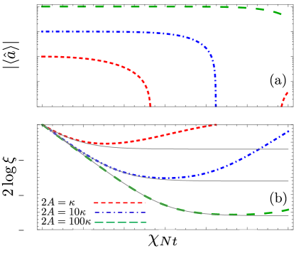
Figure 4: (a) Absolute value of the cavity field coherence $|\langle\hat{a}\rangle|$ versus time , and (b) evolution in dB for the squeezing parameter $\xi^{2}$. Three different values of the drive intensity have been considered: $2A=\kappa,10\kappa,100\kappa$ (reported in the legend). The rest of the parameters are $Ng_{\rm eff}=\kappa=\gamma=1$. The time scale, $(\chi N)^{-1}$ is given by Eq. (13). The solid grey curves describe the results obtained using the analytical result in Eq. (14).

III Implementation

Eq. (14) establishes that $\xi^{2}$ decays exponentially to $\gamma/(\chi N)$. This term can be rewritten in terms of both, single qubit-cavity coupling and average number of photons in a driven cavity ($n_{\rm ph}$) such that

$$\frac{\gamma}{\chi N}\sim\frac{\gamma}{gN\sqrt{n_{\rm ph}}(g/\omega_{q})^{2}}.$$ (15)

Notice that $\sqrt{n_{\rm ph}}=2A/\kappa$ ,where $A$ is the drive amplitude. As said, in the pros side is the $N^{-1}$ dependence, together with the enhancement due to the initial driving. However, in the cons we have the ratio $(g/\omega_{q})^{2}$. This trade off is better understood by comparing our protocol with similar ones. We consider a recent and optimized protocol Lewis-Swan et al. (2018), which is limited by spins dissipation as

$$\xi^{2}_{\rm Ref.[13]}\sim\frac{\sqrt{\kappa\gamma/N}}{g}\,,$$ (16)

so that our scaling in terms of the latter will be

$$\xi^{2}\sim\left(\frac{\omega_{q}}{g}\right)^{2}\sqrt{\frac{\gamma}{\kappa Nn_{\rm ph}}}\xi^{2}_{\rm Ref.[13]}.$$ (17)

Hence, we need to search for architectures where: (i) it is possible to couple a large number of effective spins to a single-mode cavity, (ii) together with a non-negligible single-spin normalized coupling strength ($g/\omega_{q}$) and (iii) strong cavity pumping is feasible.

Several cavity-QED architectures can satisfy the above criteria. Here, we discuss the coupling between single molecular magnets and coplanar waveguide cavities. Using nano-constrictions together with magnetic molecules, single spin-cavity coupling strengths of the order of $g/\omega_{q}\sim(10^{-4}-10^{-3})$ can be achieved both for $S=1/2$ and higher spin molecules having decoherence times up to ms Jenkins et al. (2013, 2016). Moreover, since the molecules are nano-sized objects, a macroscopic number of them can be coupled to the coplanar waveguide cavity. In addition, the protocol assumes that turning on- and off-resonance the spins indus the fastest time scale in the problem. Following Jenkins et al. (2016), in our simulations we consider realistic numbers $g/\omega_{q}\sim 10^{-4}$ and $\gamma\sim\kappa\sim 10^{-5}$. Then, placing $N\sim 10^{9}$ of those spins we get the parameters used in Fig. 4. Finally, we must consider the maximum power admitted in the nanoconstrictions. Experiments Jenkins et al. (2014) showed that $P_{\rm in}=-40$ dB (which corresponds to a number of photons $n_{\rm ph}=10^{12}$) can be safely used. Setting these realistic parameters we can get $g_{\rm eff}N=\gamma=\kappa$ obtaining $\xi^{2}=-30$ dB as shown in Fig. 4. These numbers are obtained within our effective theory, which has also been verified for tens of qubits, although, further studies including large-scale numerical calculations based on the full quantum are needed.

IV Conclusions

In this letter we have generalized the one photon-two atom process in cavity-QED to many atoms. In doing so, we have introduced a novel way for generating many-body spin-spin interactions. This yields a two-axis twisting-like interaction among the spins. Note that the mechanism is a resonant process involving real photons which facilitates the control of the effective interaction. We have shown that, already at the single-photon limit, a sizeable squeezing is produced.

Moreover, we showed that by strongly driving the cavity, the squeezing scales as $\sim 1/N$, corresponding to the Heisenberg limit. We calculated that reaching $-30$ dB is already possible with the spin-cavity and decoherence rates reported for magnetic molecules coupled to superconducting circuit resonators. However, this result is obtained after a number of approximations and thus requires confirmation by further analysis.

Our results could be implemented in various platforms, including several cavity-QED systems; although the on-chip device analyzed here can be particularly advantageous for practical applications. Here, we focused on generating squeezing, however, the novel spin-spin interaction found here can expand the possibilities for exploring many-body and nonlinear quantum physics Stassi et al. (2017).

Appendix A Derivation of the effective Hamiltonian: Two-level atoms case

In order to derive the effective Hamiltonian in Eq. (2) (see the main text), we start from Eq. (1). We first rewrite it in the basis where the qubits Hamiltonian (in the presence of interaction) is diagonal. We obtain

$$\hat{H}=\omega_{q}\hat{J}_{z}+\omega_{c}\hat{a}^{\dagger}\hat{a}+2g(\hat{a}+\hat{a}^{\dagger})(\cos\theta\hat{J}_{x}+\sin\theta\hat{J}_{z})\,,$$ (18)

where $2\hat{J}_{\alpha}=\sum_{i}\hat{\sigma}_{\alpha}^{i}$ ($\alpha=x,y,z$). Notice that the flux offset, is now encoded in the angle $\theta=\arctan(\epsilon/\Delta)$. System Hamiltonian Eq. (18) can reads as sum of two elements: a non-interacting part $\hat{H}_{0}=\omega_{q}\hat{J}_{z}+\omega_{c}\hat{a}^{\dagger}\hat{a}$ which describes the bare energy of the system and the light-matter interaction potential part $\hat{H}_{I}=2g(\hat{a}+\hat{a}^{\dagger})(\cos\theta\hat{J}_{x}+\sin\theta\hat{J}_{z})$.

We now apply the generalized James’effective Hamiltonian method Shao et al. (2017) which at the third order, neglecting the time dependent terms (RWA), gives the effective interaction Hamiltonian [Eq. (15) of Ref. Shao et al. (2017)]

$$\begin{split}\hat{H}_{\rm eff}=&-\left[\hat{h}_{1}\hat{h}_{2}^{{\dagger}}\hat{h}_{1}+\hat{h}_{1}^{{\dagger}}\hat{h}_{2}\hat{h}_{1}^{{\dagger}}\right]+\frac{1}{2}\left[\hat{h}_{1}\hat{h}_{1}\hat{h}_{2}^{{\dagger}}+\hat{h}_{1}^{{\dagger}}\hat{h}_{1}^{{\dagger}}\hat{h}_{2}+\hat{h}_{2}^{{\dagger}}\hat{h}_{1}\hat{h}_{1}+\hat{h}_{2}\hat{h}_{1}^{{\dagger}}\hat{h}_{1}^{{\dagger}}\right]-\frac{1}{2}\left[\hat{h}_{1}\hat{h}_{3}^{{\dagger}}\hat{h}_{2}+\hat{h}_{2}\hat{h}_{3}^{{\dagger}}\hat{h}_{1}+\hat{h}_{2}^{{\dagger}}\hat{h}_{3}\hat{h}_{1}^{{\dagger}}+\hat{h}_{1}^{{\dagger}}\hat{h}_{3}\hat{h}_{2}^{{\dagger}}\right]\\ &+\frac{1}{3}\left[\hat{h}_{1}\hat{h}_{2}\hat{h}_{3}^{{\dagger}}+\hat{h}_{1}^{{\dagger}}\hat{h}_{2}^{{\dagger}}\hat{h}_{3}+\hat{h}_{3}^{{\dagger}}\hat{h}_{2}\hat{h}_{1}+\hat{h}_{3}\hat{h}_{2}^{{\dagger}}\hat{h}_{1}^{{\dagger}}\right]+\frac{1}{6}\left[\hat{h}_{2}\hat{h}_{1}\hat{h}_{3}^{{\dagger}}+\hat{h}_{2}^{{\dagger}}\hat{h}_{1}^{{\dagger}}\hat{h}_{3}+\hat{h}_{3}^{{\dagger}}\hat{h}_{1}\hat{h}_{2}+\hat{h}_{3}\hat{h}_{1}^{{\dagger}}\hat{h}_{2}^{{\dagger}}\right]\;,\end{split}$$ (19)

where $\hat{h}_{1}=g\cos{\theta}\,\hat{a}^{{\dagger}}\sum_{i}\hat{\sigma}_{-}^{i}$, $\hat{h}_{2}=g\sin\theta\,\hat{a}^{{\dagger}}\sum_{i}\hat{\sigma}_{z}^{j}$ and $\hat{h}_{3}=g\cos\theta\,\hat{a}^{{\dagger}}\sum_{i}\hat{\sigma}_{+}^{i}$. Replacing $\hat{h}_{i}$ into Eq. (19), adopting normal ordering for the photonic operators and neglecting higher-order terms involving two destruction or creation photon operators, we obtain

$$\begin{split}\hat{H}_{\rm eff}=&-\frac{2g^{3}\cos^{2}\theta\sin\theta}{\omega^{2}_{\rm q}}\left[\hat{a}\sum_{jk}\hat{\sigma}_{+}^{j}\hat{\sigma}_{+}^{k}+\hat{a}^{{\dagger}}\sum_{jk}\hat{\sigma}_{-}^{j}\hat{\sigma}_{-}^{k}\right]\\ &-\frac{g^{3}\cos^{2}\theta\sin\theta}{2\omega^{2}_{\rm q}}\left[2\hat{a}\sum_{ijk}\hat{\sigma}_{+}^{j}\hat{\sigma}_{+}^{k}\hat{\sigma}_{z}^{i}+4\hat{a}\sum_{jk}\hat{\sigma}_{+}^{j}\hat{\sigma}_{+}^{k}+2\hat{a}\sum_{ijk}\hat{\sigma}_{-}^{j}\hat{\sigma}_{-}^{k}\hat{\sigma}_{z}^{i}-4\hat{a}\sum_{jk}\hat{\sigma}_{-}^{j}\hat{\sigma}_{-}^{k}\right]\\ &+\frac{2g^{3}\cos^{2}\theta\sin\theta}{3\omega^{2}_{\rm q}}\left[\hat{a}\sum_{ijk}\hat{\sigma}_{+}^{j}\hat{\sigma}_{+}^{k}\hat{\sigma}_{z}^{i}+2\hat{a}\sum_{jk}\hat{\sigma}_{+}^{j}\hat{\sigma}_{+}^{k}+\hat{a}\sum_{ijk}\hat{\sigma}_{-}^{j}\hat{\sigma}_{-}^{k}\hat{\sigma}_{z}^{i}-2\hat{a}\sum_{jk}\hat{\sigma}_{-}^{j}\hat{\sigma}_{-}^{k}\right]\\ &+\frac{g^{3}\cos^{2}\theta\sin\theta}{3\omega^{2}_{\rm q}}\left[\hat{a}\sum_{ijk}\hat{\sigma}_{+}^{j}\hat{\sigma}_{+}^{k}\hat{\sigma}_{z}^{i}+4\hat{a}\sum_{jk}\hat{\sigma}_{+}^{j}\hat{\sigma}_{+}^{k}+\hat{a}\sum_{ijk}\hat{\sigma}_{-}^{j}\hat{\sigma}_{-}^{k}\hat{\sigma}_{z}^{i}\right]\,.\end{split}$$ (20)

Given Eq. (20), after some algebra, we obtain the effective interaction Hamiltonian in terms of the collective lowering and raising spin operators $\hat{J}_{\pm}=\sum_{i}\hat{\sigma}^{i}_{\pm}$

$$\hat{H}_{\rm eff}=-\frac{4g^{3}\cos^{2}\theta\sin\theta}{3\omega^{2}_{\rm q}}\left(\hat{a}\hat{J}_{+}^{2}+\hat{a}^{{\dagger}}\hat{J}_{-}^{2}\right)\,.$$ (21)

We note that the the resulting effective interaction Hamiltonian Eq. (21) does not depend on the Pauli operators $\hat{J}_{z}$.

Equation (21) displays the effective interaction Hamiltonian, describing the simultaneous generation of two excitations in an ensamble constituted by an arbitrary number $N$ of identical atoms, by one photon absorption. The effective interaction Hamiltonian Eq. (21) is responsible for the coupling between the eigenvectors $|{\color[rgb]{1,0,1}0},ggg..{\color[rgb]{1,0,1}e}..{\color[rgb]{1,0,1}e}..ggg..\rangle$ and $|{\color[rgb]{1,0,1}1},ggg..{\color[rgb]{1,0,1}g}..{\color[rgb]{1,0,1}g}..ggg..\rangle$. In terms of the angular momentum notation, they can be written as $|0,j,-j+2\rangle$ and $|1,j,-j\rangle$, respectively. More generally, this Hamiltonian couples states differing by two-qubit excitations: $|j,m\rangle\leftrightarrow|j,m+2\rangle$. The effective resonant coupling between these eigenstates, for $m=-j$ is

$$\langle 0,j,-j+2|H_{\rm eff}|1,j,-j\rangle=\frac{4g^{3}\cos^{2}\theta\sin\theta}{3\omega^{2}_{\rm q}}\sqrt{2N(N-1)}\,.$$ (22)

A.1 Derivation of the effective Hamiltonian: $\Delta$-like three-level atoms case

It has been shown Zhao et al. (2017) that it is possible to simultaneously excite two atoms by using a cavity-assisted Raman process in combination with a cavity-photon-mediated interaction. We generalize this analysis to a system of many atoms. Specifically, we consider a system of $N$ $\Delta$-like three-level atoms interacting with a single mode optical resonator Liu and et al. (2005); Zhao et al. (2017). The total Hamiltonian is $\hat{H}_{\Delta}=\hat{H}_{c}+\hat{H}_{0}+\hat{H}_{I}$, being

$$\hat{H}_{c}=\omega_{c}\hat{a}^{\dagger}\hat{a}\,,$$ (23)

the energy of the cavity,

$$\hat{H}_{0}=\sum_{i}\left(\omega_{g}\hat{\sigma}^{(i)}_{gg}+\omega_{e}\hat{\sigma}^{(i)}_{ee}+\omega_{s}\hat{\sigma}^{(i)}_{ss}\right)\,,$$ (24)

the energy of an ensemble of identical three-level ($g,e,s$) atoms (here, $\hat{\sigma}^{i}_{mn}=|m\rangle_{i}{}_{i}\langle n|$, where $|m\rangle_{i}$ is a generic eigenstate of the three-level atom with $m,n=g,e,s$), and finally,

$$\hat{H}_{I}=\hat{a}\sum^{N}_{i=1}\left(g_{ge}\hat{\sigma}^{(i)}_{eg}+g_{gs}\hat{\sigma}^{(i)}_{sg}+g_{es}\hat{\sigma}^{(i)}_{se}\right)+{\rm H.c.}\,$$ (25)

is the interaction Hamiltonian part. The term $\hat{\sigma}^{(i)}_{mn}=|m\rangle\langle n|$ is a transition operator for the $i$-th three-level atom, while $g_{mn}$ is the corresponding transition matrix elements. Assuming that the system operates in the dispersive regime: $|\Delta_{mn}|\gg g_{nm}$, where $\Delta_{mn}=\omega_{mn}-\omega_{c}$ and $\omega_{mn}=\omega_{m}-\omega_{n}$ denote the transition frequencies, it is possible to derive the effective Hamiltonian applying a unitary transformation able to eliminate the direct atom-cavity coupling

$$\hat{H}_{\rm eff}=e^{-\hat{X}}\hat{H}_{\Delta}\,e^{\hat{X}}\,,$$ (26)

where

$$\hat{X}=\sum^{N}_{i=1}\left(\frac{g_{ge}}{\Delta_{eg}}\hat{\sigma}^{(i)}_{eg}+\frac{g_{es}}{\Delta_{se}}\hat{\sigma}^{(i)}_{se}+\frac{g_{gs}}{\Delta_{sg}}\hat{\sigma}^{(i)}_{sg}-{\rm H.c.}\right)\,.$$ (27)

Keeping terms up to the third order in the interaction Hamiltonian, assuming that no atom is initially in the $|s\rangle$ state, assuming $\omega_{c}\simeq 2\omega_{eg}$, and including only the time-independent terms (in the Heisenberg picture), we obtain the effective Hamiltonian

$$\hat{H}_{\rm eff}=g_{\rm eff}\left(\hat{a}\hat{J}_{+}^{2}+\hat{a}^{{\dagger}}\hat{J}_{-}^{2}\right)\,,$$ (28)

with the resulting effective coupling strength

$$g_{\rm eff}=\frac{g_{ge}g_{gs}g_{se}}{3\Delta_{ig}\Delta_{ie}{\rm\Delta}_{eg}}(3\Delta_{ig}-\omega_{eg})\,.$$ (29)

Notice that in Eq. (28) $\hat{J}_{+}=\sum_{i}\hat{\sigma}^{(i)}_{eg}$.

Appendix B Comparison of energy levels and system dynamics obtained using the effective and the full models.

Here we start comparing the lowest energy levels [see Fig. 2], obtained by using the effective Hamiltonian in Eq. (2), with the ones calculated by using the full system Hamiltonian in Eq. (18) (which is equivalent to Eq. (1)).

Figure 5(a) shows the lowest energy levels of the full Hamiltonian (blue solid curves) and those obtained diagonalizing the effective Hamiltonian (gray dashed curves) as a function of $\omega_{c}/\omega_{q}$, calculated for $N=40$ qubits and using an individual coupling strength $g/\omega_{q}=0.03$. Since the considered effective model does not include the renormalization of the bare energy levels induced by the light-matter interaction in the dispersive regime, the bare transition energy of the spin has been used as the only fitting parameter. A ladder of well-aligned avoided level crossings at $\omega_{c}\simeq 2\omega_{q}$ (highlighted with color circles) are clearly visible. Panels (b-e) show an enlarged view of the first four avoided level crossings, indicated by circles in panel (a).

We observe a number of interesting features: (i) the four avoided level crossings in the figure [see also the enlarged views in panels (b-e)] are well aligned [see the vertical dashed red line in (a)], all at the same value of $\omega_{c}/\omega_{q}$. This vertical alignment in (a) is also preserved for (not shown) the higher energy avoided crossings for values $\omega_{/}\omega_{q}$ well below $N$; (ii) the agreement between the displayed levels obtained using the full and the effective models is good for values of $\omega_{c}/\omega_{q}\simeq 2$ around the minima of the avoided level crossings (resonance condition); (iii) the agreement is less good moving away from the resonance condition. This is simply due to the dependence (not taken into account) of the energy shifts on the bare cavity frequency. In Figs. 5(f-i) we plot the same first four avoided level crossings for $N=80$ qubits, decreasing the individual coupling strength $g/\omega_{q}=0.02355$ in order to keep constant the energy splittings. Clearly, both the full and effective models are still in good agreement at $\omega_{c}\simeq 2\omega_{q}$.

As a further check, we now analyze the free system evolution considering, as initial condition, a superposition state of the system ground state and a one-photon state with all the spins in their ground state (see the main paper Sec. II.1). All the parameters used here coincide with those used to obtain the results in Fig. 3(a). Figure 6 displays such a comparison. Specifically, the continuous curves describe the mean number of cavity photons (blue) as well as the mean excitation number for the spin system (black), and the squeezing parameter (red) obtained using Eq. (1) (the solid curves show the numerical calculations). The dashed curves in Fig. 6 correspond to the analytical calculations displayed in Fig. 3(a). The agreement between the two sets of curves (dashed and continuous curves in Fig. 6) is very good, showing that the effective Hamiltonian is able to describe well this interacting system under the resonant condition $\omega_{c}\simeq 2\omega_{q}$, at least for a moderate light-matter interaction strength.

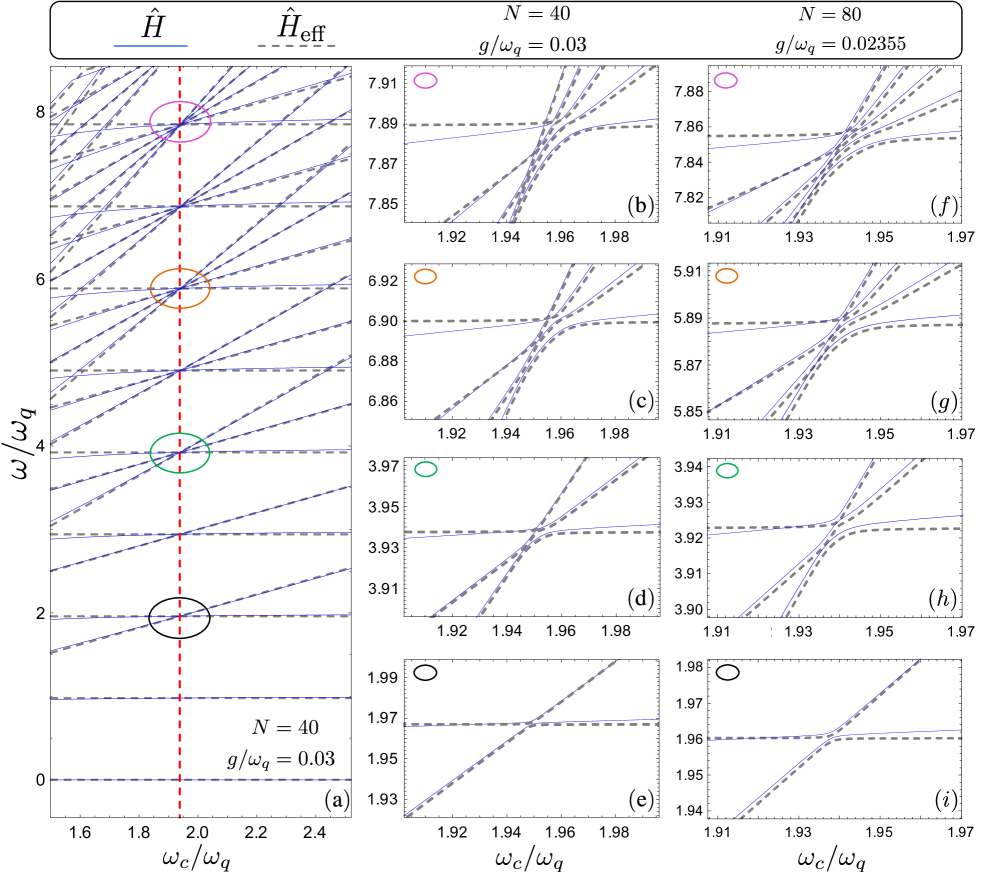
Figure 5: (a) Lowest energy levels of the full (blue solid curves) and the effective Hamiltonian (grey dashed curves) as a function of $\omega_{c}/\omega_{q}$, obtained for $N=40$ qubits and individual coupling strength $g/\omega_{q}=0.03$. Panels 5(b-e) display an enlarged view of the first four avoided level crossings [indicated by colored circles in panel (a)]. Panels 5(f-i) report the same first four avoided level crossings, obtained for $N=80$ qubits, decreasing the individual coupling strength ($g/\omega_{q}=0.02355)$ in order to keep constant the energy splittings.

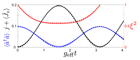
Figure 6: Free time evolution of the interacting light-matter system, considering $N=10$ effective spins for $\omega_{c}=2\omega_{q}$. The initial state is a superposition of the system ground state and a one-photon state with all the spins in their ground state (see the main paper). The continuous curves describe the mean number of cavity photons (blue) as well as the mean excitation number for the spin system (black), and the squeezing parameter (red) obtained using Eq. (1) (numerical calculation). The dashed curves correspond to the analytical results displayed in Fig. 3(a) for the effective Hamiltonian Eq. (2).

Appendix C Dissipation

The Linblad dissipators for a collection of two level systems inside a cavity have been discussed in Ref. Gelhausen et al. (2017). In this appendix we develop a similar theory adapting it to our case. We assume that the ensemble of spins occupies a small volume, compared to the cavity-mode wavelength. This is the case for the implementation discussed in the main text. With this assumption, both the cavity and atomic decays can be cast in the Lindblad form Gelhausen et al. (2017)

$$\kappa\mathcal{D}[\hat{a}] =\kappa\big{(}2\hat{a}\hat{\varrho}\hat{a}^{\dagger}-\{\hat{a}^{\dagger}\hat{a},\hat{\varrho}\}\big{)}$$ (30)

$$\gamma\mathcal{D}[\hat{\sigma}] =\gamma\sum_{i}\hat{\sigma}_{-}^{i}\hat{\varrho}\hat{\sigma}^{i}_{+}-\frac{1}{2}\{\hat{\sigma}_{+}^{i}\hat{\sigma}_{+}^{i},\hat{\varrho}\}\,.$$ (31)

Here, $\gamma$ and $\kappa$ are the atomic and cavity decay rates, respectively. Taking the Fourier transform,

$$\hat{\sigma}^{k}_{+}=\frac{1}{\sqrt{N}}\sum_{j}e^{ikj}\hat{\sigma}^{j}_{k}$$ (32)

we notice that

$$\hat{\sigma}^{0}_{\pm}=\frac{1}{\sqrt{N}}\hat{J}_{\pm}\;.$$ (33)

Using Eq. (32), the single-site dissipative terms becomes:

$$\sum_{i}\hat{\sigma}_{-}^{i}\hat{\varrho}\hat{\sigma}^{i}_{+}-\frac{1}{2}\{\hat{\sigma}_{+}^{i}\hat{\sigma}_{+}^{i},\hat{\varrho}\}$$ (34)

$$=\frac{1}{N}\sum_{k,k^{\prime}}\sum_{j}e^{i(k-k^{\prime})j}\Big{(}\hat{\sigma}_{-}^{k}\hat{\varrho}\hat{\sigma}^{k^{\prime}}_{+}-\frac{1}{2}\{\hat{\sigma}_{+}^{k^{\prime}}\hat{\sigma}_{-}^{k},\hat{\varrho}\}\Big{)}\;.$$

It is convenient to separate the zero momentum contribution which, using Eq. (33), results into:

$$\gamma\mathcal{D}[\hat{\sigma}]= \frac{\gamma}{N}\big{(}\hat{J}_{-}\hat{\varrho}\hat{J}_{+}-\frac{1}{2}\{\hat{J}_{+}\hat{J}_{-},\hat{\varrho}\}\big{)}$$ (35)

$$+\gamma\sum_{k\neq 0}\hat{\sigma}_{-}^{k}\hat{\varrho}\hat{\sigma}^{k}_{+}-\frac{1}{2}\{\hat{\sigma}_{+}^{k}\hat{\sigma}_{+}^{k},\hat{\varrho}\}\;.$$

Finally, we analize how the terms in the Hamiltonian (1) looks like in momentum space. For that, we realize that [Cf. Eq. (34)]

$$\hat{\sum}_{i}\hat{\sigma}^{i}_{+}\hat{\sigma}^{i}_{-}=\hat{\sum}_{k}\hat{\sigma}^{k}_{+}\hat{\sigma}^{k}_{-}\;.$$ (36)

Morover, the atomic-light coupling becomes

$$g(\hat{a}+\hat{a}^{\dagger})\sum_{i}\hat{\sigma}_{x}^{i}=g(\hat{a}+\hat{a}^{\dagger})(\hat{J}_{+}+\hat{J}_{-})\,.$$ (37)

As expected, the cavity only couples to the zero momentum operator. Therefore, the full dynamics (unitary + dissipative) do not mix different momenta, resulting in the QME used in the main text.

Appendix D Bosonic map in the large-$N$ limit

If $N$ is sufficiently large and the number of spin excitations satisfies the condition $\sum_{j}\langle\hat{\sigma}^{+}_{j}\hat{\sigma}_{j}^{-}\rangle\ll N$, the collective spin operator can be replaced Hümmer et al. (2012) by a bosonic mode

$$\hat{J}_{-}\equiv\sum_{i}\hat{\sigma}^{(i)}_{-}\to\sqrt{N}\,\hat{b}\;\;\;$$ (38)

$$\hat{J}_{+}\equiv\sum_{i}\hat{\sigma}^{(i)}_{+}\to\sqrt{N}\,\hat{b}^{\dagger}\,,$$ (39)

where $\hat{b}$ ($\hat{b}^{\dagger}$) is the creation (destruction) operator in the new bosonic rappresentation. Using Eq. (38), Eq. (39) and including a continuum driving term ${2A}\cos(\omega_{d}\,t)(\hat{a}+\hat{a}^{\dagger})$ (in the rotating wave approximation), the system Hamiltonian in the rotating frame becomes:

$$\hat{H}=(\omega_{c}-\omega_{d})\hat{a}^{\dagger}\hat{a}+\omega_{q}\hat{b}^{\dagger}\hat{b}+g_{\rm eff}N\;(\hat{a}\hat{b}^{\dagger\;2}+\hat{a}^{\dagger}\hat{b}^{2})+A(\hat{a}+\hat{a}^{\dagger}).$$ (40)

Notice that, since $(\hat{b}^{\dagger})^{2}|0\rangle=\sqrt{2}|2\rangle$, the anticrossing scales as $\sqrt{2}\,N$ which equals $\sqrt{2N(N-1)}$, in the $N\to\infty$ limit [Cf. Eq. (3) in the main text].

As regards the dissipators, they are global spin operators (see Appendix C). Thus, after the replacement by a bosonic mode the master equation becomes

$$\dot{\hat{\varrho}}= -i[\hat{H}_{\rm bosonic},\hat{\varrho}]$$ (41)

$$+\kappa\big{(}2\hat{a}\hat{\varrho}\hat{a}^{\dagger}-\{\hat{a}^{\dagger}\hat{a},\hat{\varrho}\}\big{)}+\gamma\big{(}\hat{b}\hat{\varrho}\hat{b}^{\dagger}-\frac{1}{2}\{\hat{b}^{\dagger}\hat{b},\hat{\varrho}\}\big{)}\,.$$

Due to the nonlinearity of the system Hamiltonian, Eq. (41) is not exactly solvable. Applying the mean-field approximation $\langle\hat{a}\hat{b}^{\dagger}\rangle\to\langle\hat{a}\rangle\langle\hat{b}^{\dagger}\rangle$, with the purpose to describe the cavity-spins interaction, we end up with a non-linear and closed set of coupled equations for the first and second moments

$$\partial_{t}\langle\hat{a}\rangle =-iNg_{\rm eff}\langle\hat{b}^{2}\rangle-iA-\frac{\kappa}{2}\langle\hat{a}\rangle$$ (42a)

$$\partial_{t}\langle\hat{b}\rangle =-iNg_{\rm eff}\langle\hat{a}\rangle\langle\hat{b}^{\dagger}\rangle-\frac{\gamma}{2}\langle\hat{b}\rangle$$ (42b)

$$\partial_{t}\langle\hat{b}^{2}\rangle =-i2Ng_{\rm eff}\langle\hat{a}\rangle(2\langle\hat{b}^{\dagger}\hat{b}\rangle+1)-\gamma\langle\hat{b}^{2}\rangle$$ (42c)

$$\partial_{t}\langle\hat{b}^{\dagger}\hat{b}\rangle =-i2Ng_{\rm eff}(\langle\hat{a}\rangle\langle\hat{b}^{\dagger\;2}\rangle-{\rm c.c.})-\gamma\langle\hat{b}^{\dagger}\hat{b}\rangle\;.$$ (42d)

Here, we are interested in computing $\xi^{2}$, wich in the bosonic limit reads Wang and Sanders (2003)

$$\xi_{N\to\infty}^{2}=1+2\Big{(}\langle\hat{b}^{\dagger}\hat{b}\rangle-|\langle\hat{b}^{2}\rangle|\Big{)}\;.$$ (43)

Besides, to findto find a closed equation of motion for $\xi$ we realize that, at the steady state, in the regime where $g_{\rm eff}\ll 1$, Eq. (42a) yields that the mean value of the cavity field coherence is a purely imaginary number, $\langle\hat{a}\rangle=-i2A/\kappa$. As a consequence, using Eq. (42c) and Eq. (42d), the mean value of the quadratic bosonic operator $\langle\hat{b}^{2}\rangle$ is a real number. Thus, we can replace $|\langle\hat{b}^{2}\rangle|\rightarrow\langle\hat{b}^{2}\rangle$ in Eq. (43) and, taking the time derivative of it we get

$$\begin{split}\frac{d\xi^{2}_{N\to\infty}}{dt}&=4\gamma\left[\langle\hat{b}^{\dagger}\hat{b}\rangle+\langle\hat{b}^{2}\rangle\right]\\ &-i4Ng_{\rm eff}\langle\hat{a}\rangle\left[1+2(\langle\hat{b}^{\dagger}\hat{b}\rangle+\langle\hat{b}^{2}\rangle\right]\;,\end{split}$$ (44)

ending up to Eq. (12) (see the main text), namely

$$\frac{d\xi^{2}}{dt}=-\big{(}i4g_{\rm eff}N\langle\hat{a}\rangle+\gamma\big{)}\xi^{2}+\gamma\,.$$ (45)

In Fig. 7, we plot an example for the time dynamics of $\xi^{2}$. Finally, in Fig. 8 we test the mean-field approximation comparing the system dynamics solved by numerical and analytical (using mean-field approximation) calculations. We compare both the mean number $\langle\hat{b}^{\dagger}\hat{b}\rangle$ and $\xi^{2}$, finding a good agreement.

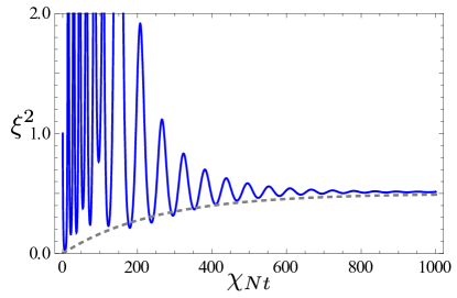
Figure 7: Dynamics for $\xi^{2}$ using Eq. (45). The parameters used are $A=10\,\kappa$ and $Ng_{\rm eff}=\kappa=\gamma=1$

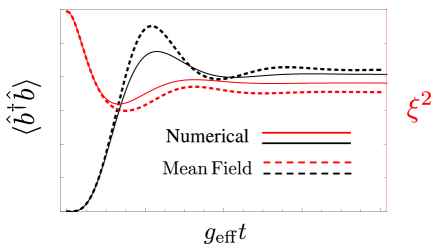
Figure 8: Comparison between the system dynamics solved by numerical calculations and using the mean-field approximation. We compare both the mean number $\langle\hat{b}^{\dagger}\hat{b}\rangle$ and $\xi^{2}$. The parameters used are $\gamma=5\times 10^{-2}\,\omega_{q}$, $A=\gamma$, $\kappa=\gamma$ and $Ng_{\rm eff}=\kappa=\gamma=1$.

Finally, for completeness, let us explore the squeezing obtained in the limit $t\to\infty$ (stationary squeezing) setting the l.h.s of Eq. (42a), Eq. (42c) and Eq. (42d) to zero. First, we introduce some dimensionless quantities, namely

$$\mathcal{A}_{\kappa}:=2{\mathcal{A}}/\kappa\,,\quad\mathcal{G}_{\gamma}:=2Ng_{\rm eff}/\gamma\,,\quad\mathcal{G}_{\kappa}:=2Ng_{\rm eff}/\kappa\,.$$ (46)

From Eq. (42c) and Eq. (42d), we solve for $\langle\hat{b}^{\dagger}\hat{b}\rangle$ in the stationary state, obtaining

$$\langle\hat{b}^{\dagger}\hat{b}\rangle=\frac{2\mathcal{G}_{\gamma}^{2}|\langle\hat{a}\rangle|^{2}}{1-4\mathcal{G}_{\gamma}^{2}|\langle\hat{a}\rangle|^{2}}\;,$$ (47)

while using Eq. (42a) and Eq. (42c) we also get

$$\langle\hat{a}\rangle=-i\mathcal{A}_{\kappa}+\mathcal{G}_{\kappa}\mathcal{G}_{\gamma}\langle\hat{a}\rangle(2\langle\hat{b}^{\dagger}\hat{b}\rangle+1)\;.$$ (48)

Combining Eq. (47) with Eq. (48) an equation for $\langle\hat{a}\rangle$ is obtained

$$\langle\hat{a}\rangle+\frac{\mathcal{G}_{\kappa}\mathcal{G}_{\gamma}\langle\hat{a}\rangle}{1-4\mathcal{G}_{\gamma}^{2}|\langle\hat{a}\rangle|^{2}}=-i\mathcal{A}_{\kappa}\,,$$ (49)

from which it follows that

$$\xi_{N\to\infty}^{2}=1+2(\langle\hat{b}^{\dagger}\hat{b}\rangle-|\langle\hat{b}^{2}\rangle|)=\frac{1}{1+2\mathcal{G}_{\gamma}|\langle\hat{a}\rangle|}\,.$$ (50)

The minimum of stationary squeezing is ${\rm min}(\xi^{2}_{N\to\infty})=1/2$. This can be understood by looking to Eq. (48). There, it is easily checked that, when $\mathcal{A}_{\kappa}\to\infty$, then $1-4\mathcal{G}_{\gamma}^{2}|\langle\hat{a}\rangle|^{2}\to 0$, thus $\xi_{N\to\infty}^{2}\to 1/2$. The latter result has been verified numerically.

References

- Kockum et al. (2017) A. F. Kockum, A. Miranowicz, V. Macrì, and F. Savasta, S.and Nori, “Deterministic quantum nonlinear optics with single atoms and virtual photons,” Phys. Rev. A 95, 063849 (2017).
- Kockum et al. (2019) A. F. Kockum, A. Miranowicz, S. De Liberato, S. Savasta, and F. Nori, “Ultrastrong coupling between light and matter,” Nat. Rev. Phys. 1, 19 (2019).
- Forn-Díaz et al. (2019) P. Forn-Díaz, L. Lamata, E. Rico, J. Kono, and E. Solano, “Ultrastrong coupling regimes of light-matter interaction,” Rev. Mod. Phys. 91, 025005 (2019).
- Ballester et al. (2012) D. Ballester, G. Romero, J. J. García-Ripoll, F. Deppe, and E. Solano, “Quantum simulation of the ultrastrong-coupling dynamics in circuit quantum electrodynamics,” Phys. Rev. X 2, 021007 (2012).
- Pedernales et al. (2015) J.S. Pedernales, I. Lizuain, S. Felicetti, G. Romero, L. Lamata, and E. Solano, “Quantum rabi model with trapped ions,” Sci. Rep. 5, 1 (2015).
- Braumüller et al. (2017) J. Braumüller, M. Marthaler, A. Schneider, A. Stehli, Ha. Rotzinger, M. Weides, and A. V. Ustinov, “Analog quantum simulation of the rabi model in the ultra-strong coupling regime,” Nat. Commun. 8, 1 (2017).
- Dingshun et al. (2018) L. Dingshun, A. Shuoming, Z. Liu, J.-N. Zhang, J. S. Pedernales, L. Lamata, E. Solano, and K. Kim, “Quantum simulation of the quantum rabi model in a trapped ion,” Phys. Rev. X 8, 021027 (2018).
- Muñoz et al. (2019) C. S. Muñoz, A. F. Kockum, A. Miranowicz, and F. Nori, “Ultrastrong-coupling effects induced by a single classical drive in jaynes-cummings-type systems,” arXiv preprint arXiv:1910.12875 (2019).
- Schwartz et al. (2011) T. Schwartz, J. A. Hutchison, C. Genet, and T. W. Ebbesen, “Reversible switching of ultrastrong light-molecule coupling,” Phys. Rev. Lett. 106, 196405 (2011).
- Kéna-Cohen et al. (2013) S. Kéna-Cohen, S. A Maier, and D. D. C. Bradley, “Ultrastrongly coupled exciton–polaritons in metal-clad organic semiconductor microcavities,” Adv. Opt. Mate. 1, 827 (2013).
- Gubbin et al. (2014) C. R. Gubbin, S. A. Maier, and S. Kéna-Cohen, “Low-voltage polariton electroluminescence from an ultrastrongly coupled organic light-emitting diode,” Appl. Phys. Lett. 104, 85 (2014).
- Mazzeo et al. (2014) M. Mazzeo, A. Genco, S. Gambino, D. Ballarini, F. Mangione, O. Di Stefano, S. Patanè, S. Savasta, D. Sanvitto, and G. Gigli, “Ultrastrong light-matter coupling in electrically doped microcavity organic light emitting diodes,” Appl. Phys. Lett. 104, 86 (2014).
- Gambino et al. (2014) S. Gambino, M. Mazzeo, A. Genco, O. Di Stefano, S. Savasta, S. Patane, D. Ballarini, F. Mangione, G. Lerario, D. Sanvitto, and G. Gigli, “Exploring light–matter interaction phenomena under ultrastrong coupling regime,” ACS Photonics 1, 1042 (2014).
- Anappara et al. (2009) A. A. Anappara, S. De Liberato, A. Tredicucci, C. Ciuti, G. Biasiol, L. Sorba, and F. Beltram, “Signatures of the ultrastrong light-matter coupling regime,” Phys. Rev. B 79, 201303 (2009).
- Genco et al. (2018) A. Genco, A. Ridolfo, S. Savasta, S. Patanè, G. Gigli, and M. Mazzeo, “Bright polariton coumarin-based oleds operating in the ultrastrong coupling regime,” Adv. Opt. Mater. 6, 1800364 (2018).
- Günter et al. (2009) G. Günter, A.A. Anappara, J. Hees, A. Sell, G. Biasiol, L. Sorba, S. De Liberato, C. Ciuti, A. Tredicucci, A. Leitenstorfer, and R. Huber, “Sub-cycle switch-on of ultrastrong light–matter interaction,” Nature 458, 178 (2009).
- Todorov et al. (2010) Y. Todorov, A. M. Andrews, R. Colombelli, S. De Liberato, C. Ciuti, P. Klang, G. Strasser, and C. Sirtori, “Ultrastrong light-matter coupling regime with polariton dots,” Phys. Rev. Lett. 105, 196402 (2010).
- Scalari et al. (2012) G. Scalari, C. Maissen, D. Turčinková, D. Hagenmüller, S. De Liberato, C. Ciuti, C. Reichl, D. Schuh, W. Wegscheider, M. Beck, and J. Faist, “Ultrastrong coupling of the cyclotron transition of a 2D electron gas to a THz metamaterial,” Science 335, 1323 (2012).
- Maissen et al. (2014) C. Maissen, G. Scalari, F. Valmorra, M. Beck, J. Faist, S. Cibella, R. Leoni, C. Reichl, C. Charpentier, and W. Wegscheider, “Ultrastrong coupling in the near field of complementary split-ring resonators,” Phys. Rev. B 90, 205309 (2014).
- Zhang et al. (2016) Q. Zhang, M. Lou, X. Li, J. L. Reno, W. Pan, J. D. Watson, M. J. Manfra, and J. Kono, “Collective non-perturbative coupling of 2d electrons with high-quality-factor terahertz cavity photons,” Nat. Phys. 12, 1005 (2016).
- Li et al. (2018) X. Li, M. Bamba, Q. Zhang, S. Fallahi, G. C. Gardner, W. Gao, M. Lou, K. Yoshioka, M. J. Manfra, and J. Kono, “Vacuum Bloch–Siegert shift in Landau polaritons with ultra-high cooperativity,” Nature Photonics 12, 324 (2018).
- Garziano et al. (2016) L. Garziano, V. Macrì, R. Stassi, O. Di Stefano, F. Nori, and S. Savasta, “One Photon Can Simultaneously Excite Two or More Atoms,” Phys. Rev. Lett. 117, 043601 (2016).
- Zhao et al. (2017) P. Zhao, X. Tan, H. Yu, S.L. Zhu, and Y. Yu, “Simultaneously exciting two atoms with photon-mediated Raman interactions,” Phys. Rev. A 95, 063848 (2017).
- Wang et al. (2017) X. Wang, A. Miranowicz, H.R. Li, and F. Nori, “Observing pure effects of counter-rotating terms without ultrastrong coupling: A single photon can simultaneously excite two qubits,” Phys. Rev. A 96, 063820 (2017).
- Tóth and Apellaniz (2014) G. Tóth and I. Apellaniz, “Quantum metrology from a quantum information science perspective,” J. Phys. A 47, 424006 (2014).
- Ma et al. (2011) J. Ma, X. Wang, C.P. Sun, and F. Nori, “Quantum spin squeezing,” Phys. Rep. 509, 89 (2011).
- Riedel et al. (2010) M.F. Riedel, P. Böhi, Y. Li, T. W. Hänsch, A. Sinatra, and P. Treutlein, “Atom-chip-based generation of entanglement for quantum metrology,” Nature 464, 1170 (2010).
- Ian et al. (2010) D.L. Ian, M. Schleier-Smith, and V. Vladan, “Implementation of Cavity Squeezing of a Collective Atomic Spin,” Phys. Rev. Lett. 104, 073604 (2010).
- Wasilewski et al. (2010) W. Wasilewski, K. Jensen, H. Krauter, J.J. Renema, M.V. Balabas, and E.S. Polzik, “Quantum Noise Limited and Entanglement-Assisted Magnetometry,” Phys. Rev. Lett. 104, 133601 (2010).
- Muessel et al. (2014) W. Muessel, H. Strobel, D. Linnemann, D.B. Hume, and M.K. Oberthaler, “Scalable Spin Squeezing for Quantum-Enhanced Magnetometry with Bose-Einstein Condensates,” Phys. Rev. Lett. 113, 103004 (2014).
- Schleier-Smith et al. (2010) M. Schleier-Smith, D.L. Ian, and V. Vladan, “States of an Ensemble of Two-Level Atoms with Reduced Quantum Uncertainty,” Phys. Rev. Lett. 104, 073604 (2010).
- Bohnet et al. (2014) J.G. Bohnet, K.C. Cox, M.A. Norcia, J. M. Weiner, Z. Chen, and J. K. Thompson, “Reduced spin measurement back-action for a phase sensitivity ten times beyond the standard quantum limit,” Nat. Photonics 8, 731 (2014).
- Vasilakis et al. (2015) G. Vasilakis, H. Shen, K. Jensen, M. Balabas, D. Salart, B. Chen, and E.S. Polzik, “Generation of a squeezed state of an oscillator by stroboscopic back-action-evading measurement,” Nat. Phys. 11, 389 (2015).
- Hosten et al. (2016a) O. Hosten, R. Krishnakumar, N.J. Engelsen, and M.A. Kasevich, “Quantum phase magnification,” Science 352, 1552 (2016a).
- Hosten et al. (2016b) O. Hosten, N.J. Engelsen, R. Krishnakumar, and M.A. Kasevich, “Measurement noise 100 times lower than the quantum-projection limit using entangled atoms,” Nature 529, 505 (2016b).
- Norcia et al. (2018) M.A. Norcia, R.J. Lewis-Swan, J.R.K. Cline, B. Zhu, A.M. Rey, and J.K. Thompson, “Cavity-mediated collective spin-exchange interactions in a strontium superradiant laser,” Science 361, 259 (2018).
- Lewis-Swan et al. (2018) R.J. Lewis-Swan, M.A. Norcia, J.R. Cline, J.K. Thompson, and A.M. Rey, “Robust Spin Squeezing via Photon-Mediated Interactions on an Optical Clock Transition,” Phys. Rev. Lett. 121, 070403 (2018).
- Opatrný (2015) T. Opatrný, “Twisting tensor and spin squeezing,” Phys. Rev. A 91, 053826 (2015).
- Liu et al. (2011) Y.C. Liu, Z.F. Xu, G.R. Jin, and L. You, “Spin Squeezing: Transforming One-Axis Twisting into Two-Axis Twisting,” Phys. Rev. Lett. 107, 013601 (2011).
- Borregaard et al. (2017) J. Borregaard, E.J. Davis, G.S. Bentsen, M.H. Schleier-Smith, and A.S. Sørensen, “One- and two-axis squeezing of atomic ensembles in optical cavities,” New J. Phys. 19, 093021 (2017).
- Chaudhry and Gong (2012) A. Z. Chaudhry and J. Gong, “Protecting and enhancing spin squeezing via continuous dynamical decoupling,” Phys. Rev. A 86, 012311 (2012).
- Agarwal et al. (1997) G. Agarwal, R. Puri, and R. Singh, “Atomic Schrödinger cat states,” Phys. Rev. A 56, 2249 (1997).
- Sørensen and Mølmer (2002) A.S. Sørensen and K. Mølmer, “Entangling atoms in bad cavities,” Phys. Rev. A 66, 022314 (2002).
- Garziano et al. (2015) L. Garziano, R. Stassi, V. Macrì, A.F. Kockum, S. Savasta, and F. Nori, “Multiphoton quantum Rabi oscillations in ultrastrong cavity QED,” Phys. Rev. A 92, 063830 (2015).
- Lambert et al. (2018) N. Lambert, M. Cirio, M. Delbecq, G. Allison, M. Marx, S. Tarucha, and F. Nori, “Amplified and tunable transverse and longitudinal spin-photon coupling in hybrid circuit-QED,” Phys. Rev. B 97, 125429 (2018).
- et al. (2013a) Ze-Liang Xiang et al., “Hybrid quantum circuits: Superconducting circuits interacting with other quantum systems,” Rev. Mod. Phys. 85, 623 (2013a).
- Schuster et al. (2010) D.I. Schuster, A.P. Sears, E. Ginossar, L. DiCarlo, L. Frunzio, J.J.L. Morton, H. Wu, G.A.D. Briggs, B.B. Buckley, D.D. Awschalom, and R.J. Schoelkopf, “High-Cooperativity Coupling of Electron-Spin Ensembles to Superconducting Cavities,” Phys. Rev. Lett. 105, 140501 (2010).
- Kubo et al. (2010) Y. Kubo, F.R. Ong, P. Bertet, D. Vion, V. Jacques, D. Zheng, A. Dréau, J.F. Roch, A. Auffeves, F. Jelezko, J. Wrachtrup, M.F. Barthe, P. Bergonzo, and D. Esteve, “Strong Coupling of a Spin Ensemble to a Superconducting Resonator,” Phys. Rev. Lett. 105, 140502 (2010).
- Wu et al. (2010) H. Wu, R.E. George, J.H. Wesenberg, K. Mølmer, D.I. Schuster, R.J. Schoelkopf, K.M. Itoh, A. Ardavan, J.J.L. Morton, and G.A.D. Briggs, “Storage of Multiple Coherent Microwave Excitations in an Electron Spin Ensemble,” Phys. Rev. Lett. 105, 140503 (2010).
- Amsüss et al. (2011) R. Amsüss, C. Koller, T. Nöbauer, S. Putz, S. Rotter, K. Sandner, S. Schneider, M. Schramböck, G. Steinhauser, H. Ritsch, J. Schmiedmayer, and J. Majer, “Cavity QED with Magnetically Coupled Collective Spin States,” Phys. Rev. Lett. 107, 060502 (2011).
- et al. (2013b) Xin-You Lü et al., “Quantum memory using a hybrid circuit with flux qubits and nitrogen-vacancy centers,” Phys. Rev. A 88, 012329 (2013b).
- et al. (2013c) Ze-Liang Xiang et al., “Hybrid quantum circuit consisting of a superconducting flux qubit coupled to a spin ensemble and a transmission-line resonator,” Phys. Rev. B 87, 144516 (2013c).
- Jenkins et al. (2013) M. Jenkins, T. Hümmer, M.J. Martínez-Pérez, J. García-Ripoll, D. Zueco, and F. Luis, “Coupling single-molecule magnets to quantum circuits,” New. J. Phys. 15, 095007 (2013).
- Jenkins et al. (2016) M.D. Jenkins, D. Zueco, O. Roubeau, G. Aromí, J. Majer, and F. Luis, “A scalable architecture for quantum computation with molecular nanomagnets,” Dalton Trans. 45, 16682 (2016).
- Garraway (2011) B.M. Garraway, “The Dicke model in quantum optics: Dicke model revisited,” Philos. Trans. Royal Soc. A 369, 1137 (2011).
- Shammah et al. (2017) N. Shammah, N. Lambert, F. Nori, and S. De Liberato, “Superradiance with local phase-breaking effects,” Phys. Rev. A 96, 023863 (2017).
- Shammah et al. (2018) N. Shammah, S. Ahmed, N. Lambert, S. De Liberato, and F. Nori, “Open quantum systems with local and collective incoherent processes: Efficient numerical simulations using permutational invariance,” Phys. Rev. A 98, 063815 (2018).
- Kirton et al. (2019) P. Kirton, M. M. Roses, J. Keeling, and E. G. Dalla Torre, “Introduction to the Dicke model: From equilibrium to nonequilibrium, and vice versa,” Adv. Quantum Technol. 2, 1800043 (2019).
- Shao et al. (2017) W. Shao, C. Wu, and X.L. Feng, “Generalized James’ effective Hamiltonian method,” Phys. Rev. A 95, 032124 (2017).
- Wineland et al. (1992) D.J. Wineland, J.J. Bollinger, W.M. Itano, F.L. Moore, and D.J. Heinzen, “Spin squeezing and reduced quantum noise in spectroscopy,” Phys. Rev. A 46, R6797 (1992).
- Wineland et al. (1994) D.J. Wineland, J.J. Bollinger, W.M. Itano, and D.J. Heinzen, “Squeezed atomic states and projection noise in spectroscopy,” Phys. Rev. A 50, 67 (1994).
- Niemczyk et al. (2010) T. Niemczyk, F. Deppe, H. Huebl, E.P. Menzel, F. Hocke, M.J. Schwarz, J.J. García-Ripoll, D. Zueco, T. Hümmer, E. Solano, A. Marx, and R. Gross, “Circuit quantum electrodynamics in the ultrastrong-coupling regime,” Nat. Phys. 6, 772 (2010).
- Kakuyanagi et al. (2016) K. Kakuyanagi, Y. Matsuzaki, C. Déprez, H. Toida, K. Semba, H. Yamaguchi, W. J. Munro, and S. Saito, “Observation of Collective Coupling between an Engineered Ensemble of Macroscopic Artificial Atoms and a Superconducting Resonator,” Phys. Rev. Lett. 117, 210503 (2016).
- Gelhausen et al. (2017) J. Gelhausen, M. Buchhold, and P. Strack, “Many-body quantum optics with decaying atomic spin states: () Dicke model,” Phys. Rev. A 95, 063824 (2017).
- Wang and Sanders (2003) X. Wang and B.C. Sanders, “Relations between bosonic quadrature squeezing and atomic spin squeezing,” Phys. Rev. A 68, 033821 (2003).
- Mandel and Wolf (1995) L. Mandel and E. Wolf, Optical coherence and quantum optics (Cambridge university press, 1995).
- Roy and Devoret (2016) A. Roy and M. Devoret, “Introduction to parametric amplification of quantum signals with Josephson circuits,” C. R. Phys. 17, 740 (2016).
- Macrì et al. (2018) V. Macrì, A. Ridolfo, O. Di Stefano, A. F. Kockum, F. Nori, and S. Savasta, “Nonperturbative dynamical Casimir effect in optomechanical systems: Vacuum Casimir-Rabi splittings,” Phys. Rev. X 8, 011031 (2018).
- Emary and Brandes (2003) C. Emary and T. Brandes, “Quantum chaos triggered by precursors of a quantum phase transition: The Dicke model,” Phys. Rev. Lett. 90, 044101 (2003).
- Dalla Torre et al. (2013) E.G. Dalla Torre, J. Otterbach, E. Demler, V. Vuletic, and M.D. Lukin, “Dissipative Preparation of Spin Squeezed Atomic Ensembles in a Steady State,” Phys. Rev. Lett. 110, 120402 (2013).
- Jenkins et al. (2014) M.D. Jenkins, U. Naether, M. Ciria, J. Sesé, J. Atkinson, C. Sánchez-Azqueta, E. Del Barco, J. Majer, D. Zueco, and F. Luis, “Nanoscale constrictions in superconducting coplanar waveguide resonators,” Appl. Phys. Lett. 105, 162601 (2014).
- Stassi et al. (2017) R. Stassi, V. Macrì, A.F. Kockum, O. Di Stefano, A. Miranowicz, S. Savasta, and F. Nori, “Quantum nonlinear optics without photons,” Phys. Rev. A 96, 023818 (2017).
- Liu and et al. (2005) Yu-xi Liu and et al., “Optical Selection Rules and Phase-Dependent Adiabatic State Control in a Superconducting Quantum Circuit,” Phys. Rev. Lett. 95, 087001 (2005).
- Hümmer et al. (2012) T. Hümmer, G. M. Reuther, P. Hänggi, and D. Zueco, “Nonequilibrium phases in hybrid arrays with flux qubits and nitrogen-vacancy centers,” Phys. Rev. A 85, 052320 (2012).