Catching and Reversing a Quantum Jump Mid-Flight

Абстракт

• A quantum system driven by a weak deterministic force while under strong continuous energy measurement exhibits quantum jumps between its energy levels (Nagourney et al., 1986, Sauter et al., 1986, Bergquist et al., 1986). This celebrated phenomenon is emblematic of the special nature of randomness in quantum physics. The times at which the jumps occur are reputed to be fundamentally unpredictable. However, certain classical phenomena, like tsunamis, while unpredictable in the long term, may possess a degree of predictability in the short term, and in some cases it may be possible to prevent a disaster by detecting an advance warning signal. Can there be, despite the indeterminism of quantum physics, a possibility to know if a quantum jump is about to occur or not? In this dissertation, we answer this question affirmatively by experimentally demonstrating that the completed jump from the ground to an excited state of a superconducting artificial atom can be tracked, as it follows its predictable ‘‘flight,’’ by monitoring the population of an auxiliary level coupled to the ground state. Furthermore, the experimental results demonstrate that the jump when completed is continuous, coherent, and deterministic. Exploiting these features, we catch and reverse a quantum jump mid-flight, thus deterministically preventing its completion. This real-time intervention is based on a particular lull period in the population of the auxiliary level, which serves as our advance warning signal. Our results, which agree with theoretical predictions essentially without adjustable parameters, support the modern quantum trajectory theory and provide new ground for the exploration of real-time intervention techniques in the control of quantum systems, such as early detection of error syndromes.

For those who gave the most but could see the least.

Цветко Ликов Цветков

(April 11, 1925 - December 11, 2017)

&

Ангелина Борисова Цветкова

(December 9, 1928 - February 2, 2016)

Overview

• Can there be, despite the indeterminism of quantum physics, a possibility to know if a quantum jump is about to occur or not?

Chapter 1 opens by introducing the notion of a quantum jump between discrete energy levels of a quantum system, a theoretical idea introduced by Bohr in 1913 (Bohr, 1913) — yet, one whose existence was experimentally observed only seven decades later (Nagourney et al., 1986, Sauter et al., 1986, Bergquist et al., 1986), in a single atomic three-level system. Section 1.1 outlines our proposal to map out the dynamics of a quantum jump from the ground, $\left|\mathrm{G}\right\rangle$, to an excited, $\left|\mathrm{D}\right\rangle$, state of a three-level superconducting system. We propose a protocol to catch quantum jumps mid-flight and, further, to reverse them prior to their completion. The proposal critically hinges on achieving near unit-measurement efficiency, as discussed, and experimentally demonstrated, in Sec. 1.2. Building on this, the catch and reverse experimental protocols and measurement results are presented in Sections 1.3 and 1.4. These results directly demonstrate that the answer to the above-posed question can indeed be in the affirmative. Section 1.4 summarizes the experimental results that demonstrate the deterministic prevention of the completion of jumps; this experiment thereby precludes quantum jumps from occurring altogether. A control experiment in which the feedback intervention does not exploit the deterministic character of the completed jumps is presented. Before proceeding to the remainder of the thesis, Section 1.5 provides a brief discussion of the main results and their implications for the hundred-year-long debate on the nature and reality of quantum jumps. The section concludes by providing an outlook for the implications of the results for future experiments. The remaining chapters, whose individually aim is described in the following paragraphs, provide further support to the main conclusions presented in Chapter 1 and devoted special attention to explicating the theory and experimental methodology of the work.

Chapter 2 develops the essential background needed to gain access to the core ideas and results of quantum measurement theory and its formulation, which lead to the catch and reverse theoretical prediction and modeling of the experiment. The basic notions of the formalism are introduced in view of specific examples. Building on this background, Chapter 3 develops the quantum trajectory description of the quantum jumps observed in the three-level atom. The basic ideas as well as the rigorous, quantitative description of the continuous, coherent, and deterministic evolution of a completed quantum jump is presented. Finally, the realistic model of the experiment including known imperfections is developed. Chapter 4 details the experimental methods, including our approach to the design of the superconducting quantum devices developed in Minev et al. (2018). Section 4.1.1 provides a nutshell introduction to this approach, referred to as the energy-participation-ratio (EPR) approach and used to design and optimize both the dissipative and Hamiltonian parameters of our circuit-quantum-electrodynamic (cQED) systems.

Chapter 5 presents the results of control experiments that further support the conclusions reached in Chapter 1. The comparison between the experimental results and the predictions of the quantum trajectory theory developed in Chapter 3 is provided in Sec. 5.5. Chapter 6 summarizes the results of this dissertation and discusses future research directions.

1Introduction and main results

If all this damned quantum jumping were really to stay, I should be sorry I ever got involved with quantum theory.

Erwin Schrödinger
Brit. J. Philos. Sci. III, 109 (1952)

Bohr conceived of quantum jumps Bohr (1913) in 1913, and while Einstein elevated their hypothesis to the level of a quantitative rule with his AB coefficient theory (Einstein, 1916, 1917), Schrödinger strongly objected to their existence (Schrödinger, 1952). The nature and existence of quantum jumps remained a subject of controversy for seven decades until they were directly observed in a single system (Nagourney et al., 1986, Sauter et al., 1986, Bergquist et al., 1986). Since then, quantum jumps have been observed in a variety of atomic (Basche et al., 1995, Peil and Gabrielse, 1999, Gleyzes et al., 2007, Guerlin et al., 2007) and solid-state (Jelezko et al., 2002, Neumann et al., 2010, Robledo et al., 2011, Vijay et al., 2011, Hatridge et al., 2013) systems. Recently, quantum jumps have been recognized as an essential phenomenon in quantum feedback control (Deléglise et al., 2008, Sayrin et al., 2011), and in particular, for detecting and correcting decoherence-induced errors in quantum information systems (Sun et al., 2013, Ofek et al., 2016).

Here, we focus on the canonical case of quantum jumps between two levels indirectly monitored by a third — the case that corresponds to the original observation of quantum jumps in atomic physics (Nagourney et al., 1986, Sauter et al., 1986, Bergquist et al., 1986), see the level diagram of Fig. 1.1a. A surprising prediction emerges according to quantum trajectory theory (see Carmichael (1993), Porrati and Putterman (1987), Ruskov et al. (2007) and Chapter 2): not only does the state of the system evolve continuously during the jump between the ground $\left|\mathrm{G}\right\rangle$ and excited $\left|\mathrm{D}\right\rangle$ state, but it is predicted that there is always a latency period prior to the jump, during which it is possible to acquire a signal that warns of the imminent occurrence of the jump (see Chapter 3 for the theoretical analysis and mathematical treatment). This advance warning signal consists of a rare, particular lull in the excitation of the ancilla state $\left|\mathrm{B}\right\rangle$. The acquisition of this signal requires the time-resolved detection of every de-excitation of $\left|\mathrm{B}\right\rangle$. Instead, exploiting the specific advantages of superconducting artificial atoms and their quantum-limited readout chain, we designed an experiment that implements with maximum fidelity and minimum latency the detection of the advance warning signal occurring before the quantum jump (see rest of Fig. 1.1).

1.1 Principle of the experiment

First, we developed a superconducting artificial atom with the necessary V-shape level structure (see Fig. 1.1a and Section 4.1). It consists, besides the ground level $\left|\mathrm{G}\right\rangle$, of one protected, dark level $\left|\mathrm{D}\right\rangle$ — engineered to not couple to any dissipative environment or any measurement apparatus — and one ancilla level $\left|\mathrm{B}\right\rangle$, whose occupation is monitored at rate $\Gamma$. Quantum jumps between $\left|\mathrm{G}\right>$ and $\left|\mathrm{D}\right>$ are induced by a weak Rabi drive $\Omega_{\mathrm{DG}}$ — although this drive might eventually be turned off during the jump, as explained later. Since a direct measurement of the dark level is not possible, the jumps are monitored using the Dehmelt shelving scheme (Nagourney et al., 1986). Thus, the occupation of $\left|\mathrm{G}\right>$ is linked to that of $\left|\mathrm{B}\right>$ by the strong Rabi drive $\Omega_{\mathrm{BG}}$ ($\Omega_{\mathrm{DG}}\ll\Omega_{\mathrm{BG}}\ll\Gamma$). In the atomic physics shelving scheme (Nagourney et al., 1986, Sauter et al., 1986, Bergquist et al., 1986), an excitation to $\left|\mathrm{B}\right\rangle$ is recorded with a photodetector by detecting the emitted photons from $\left|\mathrm{B}\right\rangle$ as it cycles back to $\left|\mathrm{G}\right\rangle$. From the detection events — referred to in the following as ‘‘clicks’’ — one infers the occupation of $\left|\mathrm{G}\right\rangle$. On the other hand, from a prolonged absence of clicks (to be defined precisely in Chapter 3), one infers that a quantum jump from $\left|\mathrm{G}\right\rangle$ to $\left|\mathrm{D}\right\rangle$ has occurred. Due to the poor collection efficiency and dead-time of photon counters in atomic physics (Volz et al., 2011), it is exceedingly difficult to detect every individual click required to faithfully register the origin in time of the advance warning signal. However, superconducting systems present the advantage of high collection efficiencies (Vijay et al., 2012, Ristè et al., 2013, Murch et al., 2013a, Weber et al., 2014, Roch et al., 2014, De Lange et al., 2014, Campagne-Ibarcq et al., 2016b), as their microwave photons are emitted into one-dimensional waveguides and are detected with the same detection efficiencies as optical photons. Furthermore, rather than monitoring the direct fluorescence of the $\left|\mathrm{B}\right\rangle$ state, we monitor its occupation by dispersively coupling it to an ancilla readout cavity. This further improves the fidelity of the detection of the de-excitation from $\left|\mathrm{B}\right\rangle$ (effective collection efficiency of photons emitted from $\left|\mathrm{B}\right\rangle$).

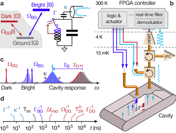
Фигура 1.1: Principle of the experiment. a, Three-level atom possessing a hidden transition (shaded region) between its ground $\left|\mathrm{G}\right\rangle$ and dark $\left|\mathrm{D}\right\rangle$ state, driven by Rabi drive $\Omega_{\mathrm{DG}}(t)$. Quantum jumps between $\left|\mathrm{G}\right\rangle$ and $\left|\mathrm{D}\right\rangle$ are indirectly monitored by a stronger Rabi drive $\Omega_{\mathrm{BG}}$ between $\left|\mathrm{G}\right\rangle$ and the bright state $\left|\mathrm{B}\right\rangle$, whose occupancy is continuously monitored at rate $\Gamma$ by an auxiliary oscillator (LC circuit on right), itself measured in reflection by continuous-wave microwave light (depicted in light blue). When the atom is in $\left|\mathrm{B}\right\rangle$, the LC circuit resonance frequency shifts to a lower frequency than when the atom is in $\left|\mathrm{G}\right\rangle$ or $\left|\mathrm{D}\right\rangle$ (effect schematically represented by switch). Therefore, the probe tone performs a $\left|\mathrm{B}\right\rangle$/not-$\left|\mathrm{B}\right\rangle$ measurement on the atom, and is blind to any superposition of $\left|\mathrm{G}\right\rangle$ and $\left|\mathrm{D}\right\rangle$. b, The actual atom and LC oscillator used in the experiment is a superconducting circuit consisting of two strongly-hybridized transmon qubits placed inside a readout resonator cavity at 15 mK. Control signals for the atom and cavity are supplied by a room-temperature field-programmable gate array (FPGA) controller. This fast electronics monitors the reflected signal from the cavity, and after demodulation and filtering, actuates the control signals. The amplifier chain includes circulators (curved arrows) and amplifiers (triangles and trapezoids). c, Frequency landscape of atom and cavity responses, overlaid with the control tones shown as vertical arrows. The cavity pull $\chi$ of the atom is nearly identical for $\left|\mathrm{G}\right\rangle$ and $\left|\mathrm{D}\right\rangle$, but markedly distinct for $\left|\mathrm{B}\right\rangle$. The BG drive is bi-chromatic in order to address the bright transition independently of the cavity state. d, Hierarchy of timescales involved in the experiment, which are required to span 5 orders of magnitude. Symbols explained in text, and summarized in Table 5.2.

The readout cavity, schematically depicted in Fig. 1.1a by an LC circuit, is resonant at $\omega_{\mathrm{C}}=8979.64\,\mathrm{MHz}$ and cooled to 15 mK. Its dispersive coupling to the atom results in a conditional shift of its resonance frequency by $\chi_{\mathrm{B}}/2\pi=-5.08\pm 0.2\,\mathrm{MHz}$ ($\chi_{\mathrm{D}}/2\pi=-0.33\pm 0.08\,\mathrm{MHz}$) when the atom is in $\left|\mathrm{B}\right\rangle$ ($\left|\mathrm{D}\right\rangle$), see Fig. 1.1c. The engineered large asymmetry between $\chi_{\mathrm{B}}$ and $\chi_{\mathrm{D}}$ together with the cavity coupling rate to the output waveguide, $\kappa/2\pi=3.62\pm 0.05\,\mathrm{MHz}$, renders the cavity response markedly resolving for $\left|\mathrm{B}\right\rangle$ vs. not-$\left|\mathrm{B}\right\rangle$, yet non-resolving (Gambetta et al., 2011, Ristè et al., 2013, Roch et al., 2014) for $\left|\mathrm{G}\right\rangle$ vs. $\left|\mathrm{D}\right\rangle$, thus preventing information about the dark transition from reaching the environment. When probing the cavity response at $\omega_{\mathrm{C}}-\chi_{\mathrm{B}}$, the cavity either remains empty, when the atom is in $\left|\mathrm{G}\right\rangle$ or $\left|\mathrm{D}\right\rangle$, or fills with $\bar{n}=5\pm 0.2$ photons when the atom is in $\left|\mathrm{B}\right\rangle$. This readout scheme yields a transduction of the $\left|\mathrm{B}\right\rangle$-occupancy signal with five-fold amplification, which is an important advantage to overcome the noise of the following amplification stages. To summarize, in this readout scheme, the cavity probe inquires: Is the atom in $\left|\mathrm{B}\right\rangle$ or not? The time needed to arrive at an answer with a confidence level of 68% (signal-to-noise ratio of 1) is $\Gamma^{-1}\approx 1/\left(\kappa\bar{n}\right)=8.8\,\mathrm{ns}$ for an ideal amplifier chain (see Chapter 3).

Importantly, the engineered near-zero coupling between the cavity and the $\left|\mathrm{D}\right\rangle$ state protects the $\left|\mathrm{D}\right\rangle$ state from harmful effects, including Purcell relaxation, photon shot-noise dephasing, and the yet unexplained residual measurement-induced relaxation in superconducting qubits (Slichter et al., 2016). We have measured the following coherence times for the $\left|\mathrm{B}\right\rangle$ state: energy relaxation $T_{1}^{\mathrm{D}}=116\pm 5\,\mathrm{\mu s}$, Ramsey coherence $T_{\mathrm{2R}}^{\mathrm{D}}=120\pm 5\,\mathrm{\mu s}$, and Hahn echo $T_{\mathrm{2E}}^{\mathrm{D}}=162\pm 6\,\mathrm{\mu s}$. While protected, the $\left|\mathrm{D}\right\rangle$ state is indirectly quantum-non-demolition (QND) read out by the combination of the V-structure, the drive between $\left|\mathrm{G}\right\rangle$ and $\left|\mathrm{B}\right\rangle$, and the fast $\left|\mathrm{B}\right\rangle$-state monitoring. In practice, we can access the population of $\left|\mathrm{D}\right\rangle$ using an 80 ns unitary pre-rotation among the levels followed by a projective measurement of $\left|\mathrm{B}\right\rangle$ (see Chapter 5).

Once the state of the readout cavity is imprinted with information about the occupation of $\left|\mathrm{B}\right\rangle$, photons leak through the cavity output port into a superconducting waveguide, which is connected to the amplification chain, see Fig. 1.1b, where they are amplified by a factor of $10^{12}$. The first stage of amplification is a quantum-limited Josephson parametric converter (JPC) (Bergeal et al., 2010), followed by a high-electron-mobility transistor (HEMT) amplifier at 4 K. The overall quantum efficiency of the amplification chain is $\eta=0.33\pm 0.03$. At room temperature, the heterodyne signal is demodulated by a home-built field-programmable gate array (FPGA) controller, with a 4 ns clock period for logic operations. The measurement record consists of a time series of two quadrature outcomes, $I_{\mathrm{rec}}$ and $Q_{\mathrm{rec}}$, every 260 ns, which is the integration time $T_{\mathrm{int}}$, from which the FPGA controller estimates the state of the atom in real time. To reduce the influence of noise, the controller applies a real-time, hysteretic IQ filter (see Section 5.3.1), and then, from the estimated atom state, the control drives of the atom and readout cavity are actuated, realizing feedback control.

1.2 Unconditioned monitoring of the quantum jumps

Having described the setup of the experiment, we proceed to report its results. The field reflected out of the cavity is monitored in a free-running protocol, for which the atom is subject to the continuous Rabi drives $\Omega_{\mathrm{BG}}$ and $\Omega_{\mathrm{DG}}$, as depicted in Fig. 1.1. Figure 1.2a shows a typical trace of the measurement record, displaying the quantum jumps of our three-level artificial atom. For most of the duration of the record, $I_{\mathrm{rec}}$ switches rapidly between a low and high value, corresponding to approximately 0 ($\left|\mathrm{G}\right\rangle$ or $\left|\mathrm{D}\right\rangle$) and 5 ($\left|\mathrm{B}\right\rangle$) photons in the cavity, respectively. The spike in $Q_{\mathrm{rec}}$ at $t=210\,\mathrm{\mu s}$ is recognized by the FPGA logic as a short-lived excursion of the atom to a higher excited state (see Section 5.3.1). The corresponding state of the atom, estimated by the FPGA controller, is depicted by the color of the dots. A change from $\left|\mathrm{B}\right\rangle$ to not-$\left|\mathrm{B}\right\rangle$ is equivalent to a ‘‘click’’ event, in that it corresponds to the emission of a photon from $\left|\mathrm{B}\right\rangle$ to $\left|\mathrm{G}\right\rangle$, whose occurrence time is shown by the vertical arrows in the inferred record $\mathrm{d}N\left(t\right)$ (top). We could also indicate upward transitions from $\left|\mathrm{G}\right\rangle$ to $\left|\mathrm{B}\right\rangle$, corresponding to photon absorption events (not emphasized here), which would not be detectable in the atomic case.

In the record, the detection of clicks stops completely at $t=45\,\mathrm{\mu s}$, which reveals a quantum jump from $\left|\mathrm{G}\right\rangle$ to $\left|\mathrm{D}\right\rangle$. The state $\left|\mathrm{D}\right\rangle$ survives for $90\,\mathrm{\mu s}$ before the atom returns to $\left|\mathrm{G}\right\rangle$ at $t=135\,\mathrm{\mu s}$, when the rapid switching between $\left|\mathrm{G}\right\rangle$ and $\left|\mathrm{B}\right\rangle$ resumes until a second quantum jump to the dark state occurs at $t=350\,\mathrm{\mu s}$. Thus, the record presents jumps from $\left|\mathrm{G}\right\rangle$ to $\left|\mathrm{D}\right\rangle$ in the form of click interruptions.

In Fig. 1.2b, which is based on the continuous tracking of the quantum jumps for 3.2 s, a histogram of the time spent in not-$\left|\mathrm{B}\right\rangle$, $\tau_{\operatorname{not-B}}$, is shown. The panel also shows a fit of the histogram by a bi-exponential curve that models two interleaved Poisson processes. This yields the average time the atom rests in $\left|\mathrm{G}\right\rangle$ before an excitation to $\left|\mathrm{B}\right\rangle$, $\Gamma_{\mathrm{BG}}^{-1}=0.99\pm 0.06\,\mathrm{\mu s}$, and the average time the atom stays up in $\left|\mathrm{D}\right\rangle$ before returning to $\left|\mathrm{G}\right\rangle$ and being detected, $\Gamma_{\mathrm{GD}}^{-1}=30.8\pm 0.4\,\mathrm{\mu s}$. The average time between two consecutive $\left|\mathrm{G}\right\rangle$ to $\left|\mathrm{D}\right\rangle$ jumps is $\Gamma_{\mathrm{DG}}^{-1}=220\pm 5\thinspace\mathrm{\mu s}$. The corresponding rates depend on the atom drive amplitudes ($\Omega_{\mathrm{DG}}$ and $\Omega_{\mathrm{BG}}$) and the measurement rate $\Gamma$ (see Chapter 3). Crucially, all the rates in the system must be distributed over a minimum of 5 orders of magnitude, as shown in Fig. 1.2d.

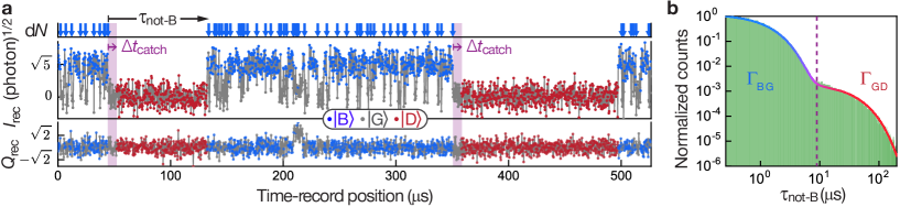
Фигура 1.2: Unconditioned monitoring of quantum jumps in the 3-level system. a, Typical measurement of integrated, with duration $T_{\mathrm{int}},$ quadratures $I_{\mathrm{rec}}$ and $Q_{\mathrm{rec}}$ of signal reflected from readout cavity as a function of time. The color of the dots (see legend) denotes the state of the atom estimated by a real-time filter implemented with the FPGAs (see Section 5.3.1). On top, the vertical arrows indicate ‘‘click’’ events ($\mathrm{d}N$) corresponding to the inferred state changing from $\left|\mathrm{B}\right\rangle$ to not-$\left|\mathrm{B}\right\rangle$. The symbol $\tau_{\operatorname{not-B}}$ corresponds to the time spent in not-$\left|\mathrm{B}\right\rangle$, which is the time between two clicks minus the last duration spent in $\left|\mathrm{B}\right\rangle$. An advance warning that a jump to $\left|\mathrm{D}\right\rangle$ is occurring is triggered when no click has been observed for a duration $\Delta t_{\mathrm{catch}}$, which is chosen between 1 and 12$\,\mathrm{\mu s}$ at the start of the experiment. b, Log-log plot of the histogram of $\tau_{\operatorname{not-B}}$ (shaded green) for 3.2 s of continuous data of the type of panel (a). Solid line is a bi-exponential fit defining jump rates $\Gamma_{\mathrm{BG}}=\left(0.99\pm 0.06\,\mathrm{\mu s}\right)^{-1}$ and $\Gamma_{\mathrm{GD}}=\left(30.8\pm 0.4\,\mathrm{\mu s}\right)^{-1}$.

1.3 Catching the quantum jump

Having observed the quantum jumps in the free-running protocol, we proceed to conditionally actuate the system control tones in order to tomographically reconstruct the time dynamics of the quantum jump from $\left|\mathrm{G}\right\rangle$ to $\left|\mathrm{D}\right\rangle$, see Fig. 1.3a. Like previously, after initiating the atom in $\left|\mathrm{B}\right\rangle$, the FPGA controller continuously subjects the system to the atom drives ($\Omega_{\mathrm{BG}}$ and $\Omega_{\mathrm{DG}}$) and to the readout tone ($\mathrm{R}$). However, in the event that the controller detects a single click followed by the complete absence of clicks for a total time $\Delta t_{\operatorname{catch}}$, the controller suspends all system drives, thus freezing the system evolution, and performs tomography, as explained in Section 5.2.2. Note that in each realization, the tomography measurement yields a single +1 or -1 outcome, one bit of information for a single density matrix component. We also introduce a division of the duration $\Delta t_{\operatorname{catch}}$ into two phases, one lasting $\Delta t_{\mathrm{on}}$ during which $\Omega_{\mathrm{DG}}$ is left on and one lasting $\Delta t_{\mathrm{off}}=\Delta t_{\operatorname{catch}}-\Delta t_{\mathrm{on}}$ during which $\Omega_{\mathrm{DG}}$ is turned off. As we explain below, this has the purpose of demonstrating that the evolution of the jump is not simply due to the Rabi drive between $\left|\mathrm{G}\right\rangle$ and $\left|\mathrm{D}\right\rangle$.

In Fig. 1.3b, we show the dynamics of the jump mapped out in the full presence of the Rabi drive, $\Omega_{\mathrm{GD}}$, by setting $\Delta t_{\mathrm{off}}=0$. From $3.4\times 10^{6}$ experimental realizations we reconstruct, as a function of $\Delta t_{\operatorname{catch}}$, the quantum state, and present the evolution of the jump from $\left|\mathrm{G}\right\rangle$ to $\left|\mathrm{D}\right\rangle$ as the normalized, conditional GD tomogram (see Section 5.2.2). For $\Delta t_{\operatorname{catch}}<2\,\mathrm{\mu s}$, the atom is predominantly detected in $\left|\mathrm{G}\right\rangle$ ($Z_{\mathrm{GD}}=-1$), whereas for $\Delta t_{\operatorname{catch}}>10\,\mathrm{\mu s}$, it is predominantly detected in $\left|\mathrm{D}\right\rangle$ ($Z_{\mathrm{GD}}=+1$). Imperfections, due to excitations to higher levels, reduce the maximum observed value to $Z_{\mathrm{GD}}=+0.9$ (see Section 5.5).

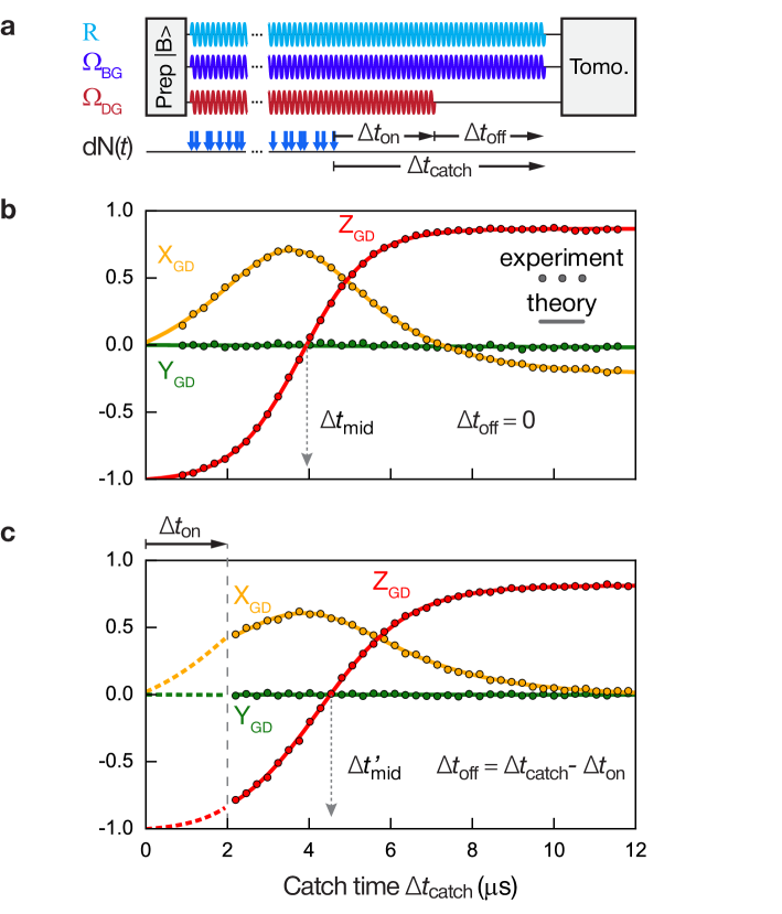
Фигура 1.3: Catching the quantum jump mid-flight. a, The atom is initially prepared in $\left|\mathrm{B}\right\rangle$. The readout tone ($\mathrm{R}$) and atom Rabi drive $\Omega_{\mathrm{BG}}$ are turned on until the catch condition is fulfilled, consisting of the detection of a click followed by the absence of click detections for a total time $\Delta t_{\mathrm{catch}}$. The Rabi drive $\Omega_{\mathrm{DG}}$ starts with $\Omega_{\mathrm{BG}}$, but can be shut off prematurely, prior to the end of $\Delta t_{\mathrm{catch}}$. A tomography measurement is performed after $\Delta t_{\mathrm{catch}}$. b & c, Conditional tomography revealing the continuous, coherent, and, surprisingly, deterministic flight (when completed) of the quantum jump from $\left|\mathrm{G}\right\rangle$ to $\left|\mathrm{D}\right\rangle$. The error bars are smaller than the size of the dots. The mid-flight time $\Delta t_{\mathrm{mid}}$ is defined by $Z_{\mathrm{GD}}=0$. The jump proceeds even when $\Omega_{\mathrm{DG}}$ is turned off at the beginning of the flight (panel c), $\Delta t_{\mathrm{on}}=2\,\mathrm{\mu s}$. Data obtained from $6.8\times 10^{6}$ experimental realizations. Solid lines: theoretical prediction (see Sec. 5.5). Dashed lines in panel c: theory curves for the $\Delta t_{\mathrm{on}}$ interval, reproduced from panel b. The data suggests that an advance-warning signal of the jump can be provided by a no-click period for catch time $\Delta t_{\mathrm{catch}}=\Delta t_{\mathrm{mid}}$, at which half of the jumps will complete.

For intermediate no-click times, between $\Delta t_{\operatorname{catch}}=2\,\mathrm{\mu s}$ and $\Delta t_{\operatorname{catch}}=10\,\mathrm{\mu s}$, the state of the atom evolves continuously and coherently from $\left|\mathrm{G}\right\rangle$ to $\left|\mathrm{D}\right\rangle$ — the flight of the quantum jump. The time of mid flight, $\Delta t_{\mathrm{mid}}\equiv 3.95\,\mathrm{\mu s}$, is markedly shorter than the Rabi period $2\pi/\Omega_{\mathrm{DG}}=50\,\mathrm{\mu s}$, and is given by the function $\Delta t_{\text{mid}}=\left(\frac{\Omega_{\mathrm{BG}}^{2}}{2\Gamma}\right)^{-1}\ln\left(\frac{\Omega_{\mathrm{BG}}^{2}}{\Omega_{\mathrm{DG}}\Gamma}+1\right)$, in which $\Omega_{\mathrm{DG}}$ enters logarithmically (see Section 3.1.1). The maximum coherence of the superposition, corresponding to $\sqrt{X_{\mathrm{GD}}^{2}+Y_{\mathrm{GD}}^{2}}$, during the flight is $0.71\pm 0.005$, quantitatively understood to be limited by several small imperfections (see Section 5.5).

Motivated by the exact quantum trajectory theory, we fit the experimental data with the analytic form of the jump evolution, $\mathrm{Z}_{\text{GD}}(\Delta t_{\operatorname{catch}})=a+b\tanh(\Delta t_{\operatorname{catch}}/\tau+c)$, $\mathrm{X}_{\text{GD}}(\Delta t_{\operatorname{catch}})=a^{\prime}+b^{\prime}\operatorname{sech}(\Delta t_{\operatorname{catch}}/\tau^{\prime}+c^{\prime})$, and $\mathrm{Y}_{\text{GD}}(\Delta t_{\operatorname{catch}})=0$. We compare the fitted jump parameters ($a,a^{\prime},b,b^{\prime},c,c^{\prime},\tau,\tau^{\prime}$) to those calculated from the theory and numerical simulations using independently measured system characteristics (see Section 5.5).

By repeating the experiment with $\Delta t_{\text{on}}=2\,\mathrm{\mu s}$, in Fig. 1.3c, we show that the jump proceeds even if the GD drive is shut off at the beginning of the no-click period. The jump remains coherent and only differs from the previous case in a minor renormalization of the overall amplitude and timescale. The mid-flight time of the jump, $\Delta t_{\mathrm{mid}}^{\prime}$, is given by an updated formula (see Chapter 3). The results demonstrate that the role of the Rabi drive $\Omega_{\mathrm{DG}}$ is to initiate the jump and provide a reference for the phase of its evolution. Note that the $\Delta t_{\mathrm{catch}}\gg\Delta t_{\mathrm{mid}}$ non-zero steady state value of $X_{\mathrm{GD}}$ in Fig. 1.3b is the result of the competition between the Rabi drive $\Omega_{\mathrm{DG}}$ and the effect of the measurement of $\left|\mathrm{B}\right\rangle$. This is confirmed in Fig. 1.3c, where $\Omega_{\mathrm{DG}}=0$, and where there is no offset in the steady state value.

The results of Fig. 1.3 demonstrate that despite the unpredictability of the jumps from $\left|\mathrm{G}\right\rangle$ to $\left|\mathrm{D}\right\rangle$, they are preceded by an identical no-click record. While the jump starts at a random time and can be prematurely interrupted by a click, the deterministic nature of the flight comes as a surprise given the quantum fluctuations in the heterodyne record $I_{\mathrm{rec}}$ during the jump — an island of predictability in a sea of uncertainty.

1.4 Reversing the quantum jump

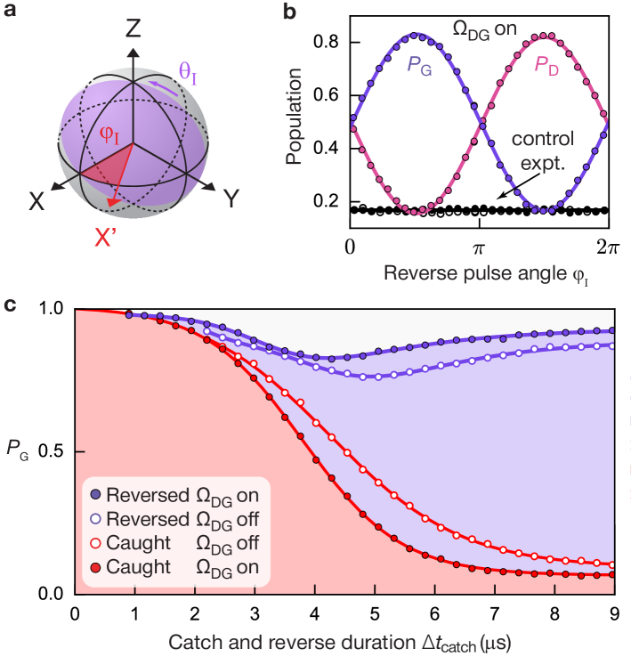
Фигура 1.4: Reversing the quantum jump mid-flight. a, Bloch sphere of the GD manifold, showing the axis X’ for the jump reversal, defined by the azimuthal angle $\varphi_{\mathrm{I}}$. The angle of the intervention pulse is $\theta_{\mathrm{I}}$. b, Success probabilities $P_{\mathrm{G}}$ (purple) and $P_{\mathrm{D}}$ (orange) to reverse to $\left|\mathrm{G}\right\rangle$ and complete to $\left|\mathrm{D}\right\rangle$ the quantum jump mid-flight at $\Delta t_{\mathrm{catch}}=\Delta t_{\mathrm{mid}}$, with $\theta_{\mathrm{I}}=\pi/2$, in the presence of the Rabi drive $\Omega_{\mathrm{DG}}$. The error bars are smaller than the size of the dots. Black dots: success probability for $\left|\mathrm{G}\right\rangle$ (closed dots) and $\left|\mathrm{D}\right\rangle$ (open dots) in a control experiment where intervention is applied at random times along the record, rather than at $\Delta t_{\mathrm{catch}}$. c, Optimal success of reverse protocol (purple) as a function of $\Delta t_{\mathrm{catch}}$. The FPGA controller is programmed with the optimal $\left\{\theta_{I}\left(\Delta t_{\mathrm{catch}}\right),\varphi_{I}\left(\Delta t_{\mathrm{catch}}\right)\right\}$. Closed and open dots correspond to $\Delta t_{\mathrm{on}}=\Delta t_{\mathrm{catch}}$ and $\Delta t_{\mathrm{on}}=2\,\mathrm{\mu s}$, respectively. Red points show the corresponding open-loop (no intervention) results from Fig. 1.3b and c.

In Fig. 1.4b, we show that by choosing $\Delta t_{\operatorname{catch}}=\Delta t_{\mathrm{mid}}$ for the no-click period to serve as an advance warning signal, we reverse the quantum jump in the presence of $\Omega_{\mathrm{DG}}$; the same result is found when $\Omega_{\mathrm{DG}}$ is off, see Section 3.1.3. The reverse pulse characteristics are defined in Fig. 1.4a. For $\varphi_{\mathrm{I}}=\pi/2$, our feedback protocol succeeds in reversing the jump to $\left|\mathrm{G}\right\rangle$ with $83.1\%\pm 0.3\%$ fidelity, while for $\varphi_{\mathrm{I}}=3\pi/2$, the protocol completes the jump to $\left|\mathrm{D}\right\rangle$, with $82.0\%\pm 0.3\%$ fidelity. In a control experiment, we repeat the protocol by applying the reverse pulse at random times, rather than those determined by the advance warning signal. Without the advance warning signal, the measured populations only reflect those of the ensemble average.

In a final experiment, we programmed the controller with the optimal reverse pulse parameters $\left\{\theta_{I}\left(\Delta t_{\mathrm{catch}}\right),\varphi_{I}\left(\Delta t_{\mathrm{catch}}\right)\right\}$, and as shown in Fig. 1.4c, we measured the success of the reverse protocol as a function of the catch time, $\Delta t_{\mathrm{catch}}$. The closed/open dots indicate the results for $\Omega_{\mathrm{DG}}$ on/off, while the solid curves are theory fits motivated by the exact analytic expressions (see Chapter 3). The complementary red dots and curves reproduce the open-loop results of Fig. 1.3 for comparison.

1.5 Discussion of main results

From the experimental results of Fig. 1.2a one can infer, consistent with Bohr’s initial intuition and the original ion experiments, that quantum jumps are random and discrete. Yet, the results of Fig. 1.3 support a contrary view, consistent with that of Schrödinger: the evolution of the jump is coherent and continuous. Noting the difference in time scales in the two figures, we interpret the coexistence of these seemingly opposed point of views as a unification of the discreteness of countable events like jumps with the continuity of the deterministic Schrödinger’s equation. Furthermore, although all $6.8\times 10^{6}$ recorded jumps (Fig. 1.3) are entirely independent of one another and stochastic in their initiation and termination, the tomographic measurements as a function of $\Delta t_{\mathrm{catch}}$ explicitly show that all jump evolutions follow an essentially identical, predetermined path in Hilbert space — not a randomly chosen one — and, in this sense, they are deterministic. These results are further corroborated by the reversal experiments shown in Fig. 1.4, which exploit the continuous, coherent, and deterministic nature of the jump evolution and critically hinge on priori knowledge of the Hilbert space path. With this knowledge ignored in the control experiment of Fig. 1.4b, failure of the reversal is observed.

In conclusion (see Chapter 6 for an expanded discussion), these experiments revealing the coherence of the jump, promote the view that a single quantum system under efficient, continuous observation is characterized by a time-dependent state vector inferred from the record of previous measurement outcomes, and whose meaning is that of an objective, generalized degree of freedom. The knowledge of the system on short timescales is not incompatible with an unpredictable switching behavior on long time scales. The excellent agreement between experiment and theory including known experimental imperfections (see Sec. 5.5) thus provides support to the modern quantum trajectory theory and its reliability for predicting the performance of real-time intervention techniques in the control of single quantum systems.

2Quantum measurement theory

In quantum physics, you don’t see what you get, you get what you see.

A.N. Korotkov
Private communication

This chapter provides a general background to the central ideas and results of quantum measurement theory. It begins with a prelude, Section 2.1, where the elementary notions of the measurement formalism are introduced. These are developed, in Sections 2.1.1 and 2.1.2, within the framework of probability theory. For simplicity, the initial discussion is concerned with measurements of classical systems. Section 2.1.3 extends the discussion to measurements of quantum systems, and it is seen that many of the concepts developed in the classical setting directly carry over. The tack of this approach makes it easy to discern the classical from the quantum aspects of measurements. The ideas and results of Sec. 2.1 are extended to time-continuous measurements in Sec. 2.2 by way of a specific example before generalizing to arbitrary systems. Specifically, we construct a microscopic description of the homodyne monitoring of a qubit, using only two-level ancillary systems. Although the time-discrete model is simple and is readily solved, it contains sufficient generality to illustrate the principal ideas of continuous quantum measurements. The concept of a stochastic path taken by the state of a monitored quantum system over time, known as its quantum trajectory, naturally emerges from the discussion. A higher degree of mathematical rigor of the description follows in Section. 2.2.3, which takes the continuous limit of our time-discrete model, thus allowing the natural development of the basic notions of stochastic calculus; in particular, the calculus of a Wiener process (Gaussian white noise) is mathematically formulated. Finally, Section 2.3 generalizes the results of the former section to formulate the general theory of quantum measurements and quantum trajectories. This framework sets the stage for the description of the quantum jumps experiment presented in Chapter 3 (see also 5). Suggestions for further reading on the formulation of quantum trajectory theory are provided in Section 2.4.

2.1 Prelude: from classical to quantum measurements

This section provides an introduction to the basic concepts of measurement theory. Before discussing a measurement of a quantum system, it is helpful to develop and to understand the description of general, disturbing classical measurements. One finds that the probabilistic formulation of these greatly parallels that of quantum measurements. In this way, it provides a closest approach to the quantum one from the simpler, classical framework. Notably, many key ideas carry over — but, with a few modifications that prove profound and lead to the departure of the quantum measurements from classical ones. For concreteness, throughout the discussion, we keep the simplest possible example in view as we develop the theory, usually based on a classical or quantum bit. While self-contained and thorough, our discussion cannot hope to be exhaustive, and hence, for further reading, we refer the reader to the references suggested in Section 2.4.

2.1.1 Classical measurement theory: basic concepts

Let us begin with the absolute minimum needed to discuss a measurement of a classical system. Leading with the example of the simplest, smallest classical system, a bit, we first establish the notions needed to describe the system and then the measurement.

The simplest, smallest classical system — a bit.

The simplest, smallest classical system is one that, at a given time, can be described by only one of two possible configurations. A concrete, familiar example is that of a coin on a table, which is either heads or tails. More generally, such a system with two possible configurations (a bit worth of information) could represent any number of physical situations; for instance, the bit could represent the tilt of a mechanical seesaw on a playground (the seesaw is tilted either to the left or to the right), or, for instance, in a classical computer, it could represent the digital logic bit corresponding to the thresholded voltage value at the output of a transistor (for example, the two configuration could be that the voltage is less than five volts or not).

Description of the system. Continuing with the coin example, the configuration of the coin is specified by a single property, corresponding to the binary question: Is the coin tails, or not? Mathematically, this property can be specified by a variable, which we will denote $S$, and which takes only one of two values. Specifically, in anticipation of the discussion of a qubit, let us choose to assign the value $S=1$ to correspond to the coin when it is tails and $S=-1$ for heads. Analogously, a general classical system is described by its configuration, which is specified by a set of variables, each of which describes an intrinsic property of the system, such as a degree of freedom. These properties and variables are known to have objective, definite values for a classical system.

From perfect to probabilistic measurements. In principle, a perfect measurement of a classical system can be performed to unambiguously obtain the values of the system variables, even without disturbing the system. As such, an observer of the system can perform measurements to determine the unambiguous configuration of the system. In this case, the observer acquires complete information about the system, and learns everything there is to know about it. If the system is also deterministic, then the observer has thus additionally gained complete knowledge of the result of all possible future measurements on the system. Under these conditions, the description of the system is exhaustive, and there isn’t much more to say about measurements. However, these ideal conditions are often not met in practice. Measurements are often imperfect, ensembles of non-identical system have to be considered, etc. These situations require a description of the system and measurements that is inherently probabilistic. This description is the concern of classical measurement theory. In the following, we first focus on the case of a probabilistic classical system, whose description is somewhat analogous to that of an ensemble of quantum systems.

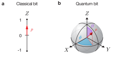
Фигура 2.1: Geometric representation of the state of a classical and quantum bit. a, State of a classical bit system represented as the one-dimensional probability vector $p$ on the line segment Z between $-1$ and $1$ (see Eq. (2.5) for the definition of Z). b, State of quantum bit (qubit) represented as the three-dimensional Bloch vector. Unlike the classical bit, the qubit has three observables (X, Y, and Z), which do not commute. The quantum state of the qubit, $\rho$, is bounded by the unit sphere. The surface of the sphere contains all pure states, which can be parametrized by the angles $\phi$ and $\theta$.

Probabilistic bit system with perfect measurements.

For concreteness, consider a coin that is prepared probabilistically, such as by a coin toss. Following the toss, an observer can perform a measurement of the coin variable $S$, which yields a measurement result. Formally, we should distinguish the measurement result obtained by the observer from the actual value of the system property $S$. For completeness, let’s denote the variable of the measurement result of $S$ as $m_{S}$. By analogy with $S$, we could assign $m_{S}=-1$ and $m_{S}=1$ to results that corresponds to heads and tails, respectively. The distinction between the measurement result $m_{S}$ and system variable $S$ is crucial for imperfect and quantum measurements. However, for simplicity, let us first proceed by assuming perfect, classical measurements where there is no confusion between $S$ and $m_{S}$, i.e, $m_{S}=S$. In this case, $m_{S}$ is redundant, and for the following discussion there is no need to insist on the distinction.

State of the system — a probability distribution. To describe the expected outcome of a measurement on the system, we introduce the concept of the system state. The state describes the probability of a configuration to be the system state. In other words, mathematically, the state is a probability distribution over all possible system configurations, which form a space known as the configuration space, denoted $\mathbb{S}$; for the bit, $\mathbb{S}\equiv\left\{S=1,S=-1\right\}$. The probability for the coin be in the tails configuration, $S=1$, is then written as $\textrm{Pr}\left[S=1\right]$. More generally, the probability that the variable $S$ of the system will have the value $s$ is $\textrm{Pr}\left[S=s\right]$; for a bit, $s\in\left\{1,-1\right\}$. This description of the classical system in terms of a probability distribution, $\textrm{Pr}\left[S=s\right]$, is analogous to the density matrix description of a quantum system. Motivated by the analogy, we express the state of the coin bit as a vector of probabilities,

$$\vec{S}\equiv\begin{pmatrix}\textrm{Pr}\left[S=1\right]\\ \textrm{Pr}\left[S=-1\right]\end{pmatrix}\,.$$ (2.1)

Keeping in mind the constraint that a measurement always yields a result, one observes that the sum of the probabilities must be one. Mathematically, the state vector $L^{1}$ norm is constrained, $\left|\vec{S}\right|_{\mathrm{L1}}=\sum_{s}\textrm{Pr}\left[S=s\right]=1$, where $\left|\cdot\right|_{\mathrm{L1}}$ denotes the $L^{1}$ norm. This property is analogous to the unit-trace property of the density matrix of a quantum state. Using this constrain, the state of the coin, Eq. (2.1), can be simplified to a single information parameter $p$, which denotes the bias of the coin,

$$\vec{S}=\begin{pmatrix}\frac{1+p}{2}\\ \frac{1-p}{2}\end{pmatrix},$$ (2.2)

The bias parameter $p$ is a number between $-1$ and 1, and, since it specifies the system state, is a quantity of central importance. It can be viewed as the classical analog of the Bloch vector of a quantum bit. In a sense, it represents a kind of one-dimensional probability vector, which constitutes a geometric representation of the system state; see Fig. 2.1a.

Operations on the system.

An operation on the system results in a change of its configuration. For the example of a coin, there are only two possible operations: i) the coin is flipped (the logical negation operation, not) or ii) the coin is left as is (the identity operation). Working within the framework of an ensemble of systems, an operation (one that is applied to all systems in the ensemble) results in a change of the state of the system that can be described by a linear map. The state of the system ensemble after the operation, denoted $S^{\prime}$, can then be written as $\vec{S}^{\prime}=U\vec{S}$, where the linear map is represented by a configuration-transition matrix, denoted $U$. For the coin, the two possible operations, the identity and not, take the following forms

$$I\equiv\begin{pmatrix}1&0\\ 0&1\end{pmatrix}\text{\ and\ }\sigma_{x}\equiv\begin{pmatrix}0&1\\ 1&0\end{pmatrix}\,,$$ (2.3)

respectively. The bit-flip Pauli matrix is denoted $\sigma_{x}$.

Perfect classical measurement of a system ensemble.

Consider the long-run average value a series of repeated measurements of the coin variable $S$, for the example of randomly prepared coins. The expected mean value of $S$ is the weighted average of the results, defined as

$$\textrm{E}\left[S\right]\equiv\sum_{s}s\textrm{Pr}\left[S=s\right]\,,$$ (2.4)

where $\textrm{E}\left[\cdot\right]$ represents ‘‘expectation value of’’ and the sum is taken over all possible values $s$ of $S$. In matrix form, recalling Eq. (2.2), Eq. (2.4) simplifies to

$$\textrm{E}\left[S\right]=\left|\sigma_{Z}\vec{S}\right|_{\mathrm{L1}}=p\,,$$ (2.5)

where $p$ is non-negative and we have introduced the measurement operator $\sigma_{Z}$, associated with the variable $S$ and given by the Pauli matrix

$$\sigma_{Z}\equiv\begin{pmatrix}1&0\\ 0&-1\end{pmatrix}\,.$$ (2.6)

The matrix formulation given by Eq. (2.5) for the expectation value of a classical measurement bears marked resemblance to that employed with quantum systems. For a measurement on a quantum bit, the expectation value of the $Z$ component of its spin is given by $\textrm{Tr}\left[\hat{\sigma}_{z}\rho\right]$, where $\rho$ is the qubit density matrix, $\hat{\sigma}_{z}$ is the Pauli Z operator, represented by the matrix given in Eq. (2.6), and $\textrm{Tr}\left[\cdot\right]$ denotes the trace function.

Concept	Symbols	Definition / Description
Basic concepts
variable	$S$,$E$	Describes intrinsic property of system, has definite value independent of measurement apparatus
variable value	$s,e$	Specific value that a variable can take
probability	$\textrm{Pr}\left[S=s\right]$	Probability that variable $S$ has value $s$
configuration	$\left\{S\right\}$,$\left\{E\right\}$,$\left\{S,E\right\}$	Set of all system variables
configuration space	$\mathbb{S}$,$\mathbb{E}$,$\mathbb{J}$	Set of all possible system configurations
state	$\vec{S},\vec{E},\vec{J}$	Probability distribution on the configuration space, represented as a vector
expectation value	$\textrm{E}\left[S\right]$	Expected (mean) value of repeated measurements of $S$, see Eq. (2.4)

Таблица 2.1: Basic concepts of classical measurement theory.

Composite system.

Extending the coin example, consider a composite system consisting of two coins. The first coin is described by the variable $S$, or in the ensemble situation, by the state $\vec{S}$, defined over the configuration space $\mathbb{S}\equiv\left\{S=1,S=-1\right\}$. The second coin is similarly described by a single variable, $E$, and a state $\vec{E}=\begin{pmatrix}\frac{1+p_{E}}{2}\\ \frac{1-p_{E}}{2}\end{pmatrix}$, where $p_{E}$ is the coin bias. Its configuration space is $\mathbb{E}\equiv\left\{E=1,E=-1\right\}$. The configuration of the composite system consists of the simultaneous specification of all variables, namely, $S$ and $E$. The set of all possible configurations of the composite system is

$$\mathbb{J} =\mathbb{S}\otimes\mathbb{E}$$ (2.7)

$$=\left\{1_{S},-1_{S}\right\}\otimes\left\{1_{E},-1_{E}\right\}$$

$$=\left\{1_{S}1_{E},\,1_{S}-1_{E},\,-1_{S}1_{E},\,-1_{S}-1_{E}\right\}\,,$$

where $\otimes$ denotes the tensor product, and where, momentarily, we have used the notation where $1_{S}$ stands for $S=1$. The state of the composite system is a probability distribution over $\mathbb{J}$, which can be represented by a 4-dimensional probability vector, $\vec{J}$. When the two subsystems are uncorrelated, the composite state is separable, and can be written as a simple product of the states of the constituent subsystems, $\vec{J}=\vec{S}\otimes\vec{E}$. However, when the subsystems are correlated, this is no longer possible. For concreteness, consider the case where the two coins are prepared randomly but always the same, the correlated randomness of the two systems is described by the composite state $\vec{J}=\left(\frac{1}{2},0,0,\frac{1}{2}\right)^{\intercal}$, where ^⊺ denotes the transposition operation. More generally, an operation that represents an interaction between the two coins results in statistical correlations between them, and thus renders the composite state inseparable. These features generally carry over to the description of composite quantum systems, but standard statistical correlations are replaced by entanglement. In the following subsection, Sec. 2.1.2, we explore the effect of an interaction between the two coins.

2.1.2 Classical toy model of system-environment interaction

For a more general discussion of measurements, it is necessary to consider the interaction of the system with another, which probes it and is often referred to as the environment. In this subsection, we consider the minimal limit of this model, where both the system and environment are bits. Further, to introduce only the essentials for now, we consider only the effect of a single interaction between the classical system and environment, and discuss the effect of the interaction on the system transfer of information. In the following subsection, Sec. 2.1.3, we consider the analogous quantum case, consisting of the interaction between a system and environment, each of which is quantum bit. In Sec. 2.2, we generalize the toy model to the time-continuous homodyne monitoring of a quantum bit.

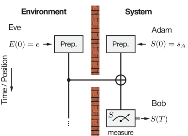
Фигура 2.2: Classical toy model of the interaction between the system and environment. Circuit of the interaction between the system, with agents Adam and Bob, and the environment, with agent Eve. Vertical lines depict the bits of the system and environment, initially prepared by Adam and Eve in the states $S\left(0\right)=s_{A}$ and $E\left(T\right)=e$, respectively. The two bits interact via a controlled-NOT (cNOT) gate. Bob measures the system at time $T$, obtaining the value $S\left(T\right)$. Brick wall depicts the lack of communication between the agents of the system and environment.

Classical toy model.

Continuing with the example of two coins, we label one as the ‘‘system’’ and the other as the ‘‘environment.’’ For definitiveness, consider the case where the system coin belongs to Adam, who aims to employ it to communicate with Bob. To achieve this, at time $t=0$, Adam prepares his coin in the configuration $S\left(0\right)=s_{A}$, where $s_{A}$ is the bit value Adam hopes to communicate. He sends the coin flying to Bob, who receives it at time $T$, and measures it to obtain the value of $S\left(T\right)$. If the coin flies undisturbed, $S\left(T\right)=S\left(0\right)$, and Bob faithfully receives Adam’s bit.

However, during its flight, the coin unavoidably interacts with a second flying coin, which belongs to an agent, Eve, who, at time $t=0$, has prepared her coin in the configuration $E\left(0\right)=e$, where $E$ is the variable describing her coin, and which is unknown to Adam and Bob. For concreteness, suppose the interaction between the two coins is described by the controlled-NOT (cNOT) gate,

$$\mathrm{cNOT}\equiv I\otimes\begin{pmatrix}1&0\\ 0&0\end{pmatrix}+\sigma_{x}\otimes\begin{pmatrix}0&0\\ 0&1\end{pmatrix}=\begin{pmatrix}1&0&0&0\\ 0&0&0&1\\ 0&0&1&0\\ 0&1&0&0\end{pmatrix}\,,$$ (2.8)

where I and $\sigma_{x}$ are defined according to Eq. (2.3). Matrices associated with operations on the system (resp: environment) are placed to the left (resp: right) of the tensor product. Given that Adam and Bob lack knowledge of Eve’s bit value, $e$, but are aware of the interaction, to what degree can they communicate, i.e., what is the effect of the interaction on the value, $S\left(T\right)$, measured by Bob? More importantly, what action can Bob undertake to undo the effect of the interaction, so as to obtain Adam’s bit, $S\left(T\right)=S\left(0\right)$?

Evolution of the state, and Bob’s information gain.

Employing the formalism developed in Section 2.1.1, the initial state of the composite system, consisting of the two coins, is described by the state vector $\vec{J}\left(0\right)=\vec{S}\left(0\right)\otimes\vec{E}\left(0\right),$ where the initial states of the system and environment are $\vec{S}\left(0\right)=\begin{pmatrix}\frac{1+s_{A}}{2}\\ \frac{1-s_{A}}{2}\end{pmatrix}$ and $\vec{E}\left(0\right)=\begin{pmatrix}\frac{1+p_{E}}{2}\\ \frac{1-p_{E}}{2}\end{pmatrix},$ respectively. The variable $p_{E}$ denotes the bias of Eve’s coin, see Eq. (2.2). Following the interaction, the composite system state is given by $\vec{J}\left(T\right)=\mathrm{cNOT\,}\vec{J}\left(0\right)$. The expected mean value of Bob’s measurement of $S\left(T\right)$, represented by the matrix $I\otimes\sigma_{z}$, is given by, recalling Eq. (2.5),

$$\textrm{E}\left[S\left(T\right)\right]=\left|\left(I\otimes\sigma_{z}\right)\vec{J}\right|_{\mathrm{L1}}=p_{E}s_{A}.$$ (2.9)

To understand Eq. (2.9), consider three limiting cases: i) Eve always prepares her coin facing up, $e=1$, corresponding to a maximal coin bias, $p_{E}=1$. Since for $e=1$ the interaction with her coin has no effect on Adam’s coin, Bob faithfully receives Adam’s bit every time, $\textrm{E}\left[S\left(T\right)\right]=s_{A}$. ii) Eve always prepares her coin facing down, $e=-1$. Since her coin bias is now $p_{E}=-1$, Bob always receives Adam’s coin flipped $\textrm{E}\left[S\left(T\right)\right]=-s_{A}$. While inconvenient for Bob, by flipping each coin he receives (a deterministic action), he could recover the bit. The effect of Eve’s coin is to change the encoding of the information, but has not resulted in its loss. iii) Eve prepares her coin completely randomly, $p_{E}=0$. On average, Bob receives no information from Adam, $\textrm{E}\left[S\left(T\right)\right]=0$! Eve has randomly scrambled the encoding of the information for each of the realizations, which, from Bob’s point of view, results in the complete loss of the initial system information encoded by Adam. More generally, for an arbitrary coin bias $p_{E}$, the information shared between Adam and Bob is characterized by the correlation between the initial and final configurations of the system, which is given by the bias of Eve’s bit, $\textrm{E}\left[S\left(T\right)S\left(0\right)\right]=p_{E}$, which can be understood as the result of information transfer between the system and environment, facilitated by the cNOT interaction, however, where the ‘‘information’’ propagating to the system from the environment is random noise.

While the transfer of information between Adam and Bob is degraded by the influence of the interaction with Eve’s bit, in principle no information has been erased, because the cNOT interaction is reversible. For the case where $p_{E}=0$, Adams bit, $s_{A}$, is not transferred to Bob at all; rather, it is encoded in the correlation between the system and environment, $\textrm{E}\left[S\left(T\right)E\left(T\right)\right]=\left|\left(\sigma_{z}\otimes\sigma_{z}\right)\vec{J}\right|_{\mathrm{L1}}=s_{A}$, which is inaccessible to Adam and Bob, who only have control over the system coin, and, hence, only access to $S$. To summarize, the interaction between the system and a randomly prepared random environment results in loss of information and injection of noise into the system, as far as the system alone is concerned. Nevertheless, from the vantage point of the composite system, no information is lost; rather, it is transferred into correlations between the system and environment.

Recovering the information.

To recover Adam’s bit, Bob requires access to Eve’s physical coin or knowledge of $e$, the specific value of her coin for each realization. First, consider the latter case, where Bob learns $e$. Recalling that $\mathrm{cNOT}^{2}=I\otimes I$, before Bob performs a measurement, he can undo the interaction effect by preparing an ancillary, third, coin with the value $e$, by employing it to perform a second cNOT operation on his coin, thus reversing the first. Applied to each realization, this procedure results in faithful communication, $\textrm{E}\left[S\left(T\right)S\left(0\right)\right]=1$. Notably, Bob can also reverse the interaction effect after performing his measurement by essentially applying the second cNOT operation virtually, i.e., when $e=1$, $s_{A}=s_{B}$, while otherwise, $s_{A}=-s_{B}$. We remark that any operations performed by Eve on her coin after the system-environment interaction have no consequences for Bob. To summarize, the examples highlights three distinct aspects regarding the recovery of information in the classical setting:

1. Eve’s physical system was not required, only information about its initial configuration, $E\left(0\right)=e$.

2. The effect of the interaction can be reversed before or after Bob’s measurement.

3. Operations on Eve’s coin subsequent to the interaction have no consequences.

All three of these features break down in the quantum setting, as discussed in the following subsection.

2.1.3 Quantum toy model

Rather than communicating with classical bits (coins), consider the situation where Adam and Bob communicate with quantum bits (qubits), and Eve too employs a qubit. Before proceeding, we briefly review the basic qubit concepts.

Quantum bit.

While the fundamental concept of classical information is the bit, which represents the minimal classical system, the fundamental concept of quantum information is the quantum bit, or qubit for short, which represents the minimal physical quantum system. A qubit has two basis states, $\left|+z\right\rangle$ and $\left|-z\right\rangle$. A pure state of the qubit is described by the state $\left|\psi\right\rangle=\cos\left(\frac{\theta}{2}\right)\left|+z\right\rangle+e^{i\phi}\sin\left(\frac{\theta}{2}\right)\left|+z\right\rangle$, where the angles $\theta$ and $\phi$, which fall in the range $0\leq\theta\leq\pi$ and $0\leq\phi\leq 2\pi$, define a point on the unit sphere, known as the Bloch sphere, see Fig. 2.1b. More generally, a statistical ensemble of pure states, a mixed qubit state is described by the density matrix

$$\rho=\frac{1}{2}\left(\hat{I}+X\hat{\sigma}_{x}+Y\hat{\sigma}_{y}+Z\hat{\sigma}_{z}\right)\,,$$ (2.10)

where $X$, $Y$, $Z$ are real numbers parameterizing the state, given by the averages of the Pauli operators, $X\equiv\textrm{Tr}\left[\hat{\sigma}_{x}\rho\right]$, et cetera, where $\textrm{Tr}\left[\cdot\right]$ denotes the trace operation. The matrix representation of the identity, $\hat{I}$, and Pauli $\hat{\sigma}_{x}$ and $\hat{\sigma}_{z}$ operators is given in Eqs. (2.3) and (2.6), while that of Pauli operator Y is $\hat{\sigma}_{y}=\begin{pmatrix}0&-i\\ i&0\end{pmatrix}$, where $i$ is the unit imaginary. The Bloch vector, $\left(X,Y,Z\right)^{\intercal}$, provides an important geometrical representation of the state of the qubit, and as discussed in Sec. 2.1.1 is the analog of the coin bias $p$. For a pure state, the Bloch vector extends to the surface of the Bloch sphere, while for mixed states, it lies in the interior. Notably, it admits the spherical parameterization:

$$X =r\sin\left(\theta\right)\cos\left(\phi\right)\,,$$

$$Y =r\sin\left(\theta\right)\sin\left(\phi\right)\,,$$

$$Z =r\cos\left(\theta\right)\,,$$ (2.11)

where the angles $\theta$ and $\phi$ are defined as for pure states and $r$ is the length of the Bloch vector, a number between 0 and 1. Notably, in the Bloch representation, mutually orthogonal state vectors are not represented by orthogonal Bloch vectors, but rather, by opposite Bloch vectors, which specify antipodal points on the sphere.

Quantum toy model.

Returning to the toy model example of the interaction between two systems (recall Fig. 2.2, which depicts the analogous classical model), we consider the case where at time $t=0$ Adam prepares his qubit in the pure state $\left|\psi\left(0\right)\right\rangle$, with corresponding Bloch vector components $X\left(0\right)$, $Y\left(0\right)$, and $Z\left(0\right)$, while Eve prepares her qubit in the pure state $\left|+x\right\rangle$, where $\left|+x\right\rangle=\frac{1}{\sqrt{2}}\left(\left|+z\right\rangle+\left|+z\right\rangle\right)$. Unlike in the classical toy model, Adam has a choice regarding the encoding of his information — the orientation of the Bloch vector, which has no classical analog. Both qubits are sent flying. A controlled-NOT interaction occurs, described by the operator $\mathrm{cNOT}=\hat{I}\otimes\left|+z\right\rangle\left\langle+z\right|+\hat{\sigma}_{x}\otimes\left|-z\right\rangle\left\langle-z\right|$, where operators on the left (resp., right) of the tensor product, denoted $\otimes$, act on the system (resp., environment). Notably, the matrix representation of the cNOT operator is the same that of the classical cNOT gate, given in Eq. (2.8). After the interaction Bob receives the system qubit, at time $T$.

Effect of the interaction before the measurement.

Before the measurement, the pure state of the composite system, $\left|\Psi\left(T\right)\right\rangle=\mathrm{cNOT}\left(\left|\psi\left(0\right)\right\rangle\left|+x\right\rangle\right)$, is, in general, inseparable — it cannot be written as a simple product of states of its component systems. On a mathematical level, this result is the same as that for the classical model; however, the interpretation and consequences are markedly distinct. Classically, the inseparability represented statistical correlations between definite configurations of the system and environment. For the quantum model, the inseparability represents entanglement between the system and environment — the system cannot be fully described without considering the environment. Generally, measurements of the entangled system are correlated with those of the environment, and the system alone cannot be represented by a pure state. The consequences of the system-environment entanglement are at the heart of quantum measurement theory.

Consider the reduced density matrix of the system qubit, found by taking the partial trace over the environment, denoted $\mathrm{Tr}_{E}\left[\cdot\right]$,

$$\rho_{S}\left(T\right)=\mathrm{Tr}_{E}\left[\left|\Psi\left(T\right)\right\rangle\left\langle\Psi\left(T\right)\right|\right]=\frac{1}{2}\begin{pmatrix}1&X\left(0\right)\\ X\left(0\right)&1\end{pmatrix}\,.$$ (2.12)

Evidently, entanglement in the composite state, the result of the interaction between the system and environment results in the loss of information from the point of view of the system. Specifically, the $Y$ and $Z$ Bloch components prepared by Adam, $Y\left(0\right)$ and $Z\left(0\right)$, are absent in $\rho_{S}\left(T\right)$, despite the deterministic preparation of the ancilla in a pure state $\left|+x\right\rangle$. However, if Adam chose to encode his information along the X component of the Bloch vector, it would propagate to Bob undisturbed by the interaction with the environment, and Bob could receive it by measuring $X$. It is the $X$ component that is preserved due to the choice of the interaction and initial pure state of the environment. Analogously to the classical case, no information is truly lost, but rather, when viewed in the broader context of the composite system, Adam’s initial $Y$ and $Z$ qubit components are encoded in the YZ, $\left\langle YZ\right\rangle\equiv\textrm{Tr}\left[\left(\hat{\sigma}_{y}\otimes\hat{\sigma}_{z}\right)\rho\right]=Y\left(0\right)$, and ZZ, $\left\langle ZZ\right\rangle\equiv\textrm{Tr}\left[\left(\hat{\sigma}_{z}\otimes\hat{\sigma}_{z}\right)\rho\right]=Z\left(0\right)$, correlations between the system and environment, respectively.

Recovering information before the measurement.

In the classical case, by learning the initial configuration of the environment, $E\left(0\right)=e$, Bob could undo the effect of the system-environment interaction and could recover the state sent by Adam before performing the measurement. In the quantum case, this is not possible. Even though Bob can know the initial state, $\left|+x\right\rangle$, of the environment and can clone it, by preparing a third ancilla qubit in the state $\left|+x\right\rangle$, he cannot use this ancilla to perform a second cNOT operation on the system so as to reverse (recall that $\mathrm{cNOT}^{2}=\hat{I}$) the cNOT performed by the environment qubit. This is a profound consequence of the entanglement between the system and environment, and has no classical analog. The only way to reverse the interaction is to use the physical qubit of the environment to perform the second cNOT operation — no clone will suffice.

Projective (von Neumann) measurement.

For a classical system described by a state of maximal knowledge, the result of any measurement can be determined with certainty. However, for a quantum system described by a state of maximal knowledge, a pure state, the result of a measurement is not, in general, determined. For definitiveness, consider the description of a perfect projective (von Neumann) measurement performed by Bob on the $Z$ component of his qubit spin, with the associated operator (observable) $\hat{\sigma}_{z}$. The measurement is described by the spectral decomposition of the observable, $\hat{\sigma}_{z}=\sum_{r}r\hat{\pi}_{r}=\hat{\pi}_{1}-\hat{\pi}_{-1}$, where $r$ is an eigenvalue, $r=1$ or $r=-1$, to which corresponds a measurement result, and $\hat{\pi}_{r}$ is the projection operator onto the eigenstate associated with $r$, $\hat{\pi}_{1}=\left|+z\right\rangle\left\langle+z\right|$ and $\hat{\pi}_{-1}=\left|+z\right\rangle\left\langle+z\right|$. The probability of obtaining an outcome corresponding to the eigenvalue $r$ is

$$\wp_{r}=\textrm{Tr}\left[\hat{\pi}_{r}\rho\right]\,.$$ (2.13)

According to the projection postulate of quantum mechanics, the measurement leads to the projection (or ‘‘collapse’’) of the system state into an eigenstate of the measurement operator. Immediately after the measurement, conditioned on the result $r$, the state of the system is

$$\rho_{r}=\frac{\hat{\pi}_{r}\rho\hat{\pi}_{r}}{\wp_{r}}\,.$$ (2.14)

The evolution due to Eq. (2.14) is markedly non-linear in the state density, which appears in the denominator, and represents a radical departure from the linear evolution encountered with Schrödinger’s equation. Further, while a perfect measurement of a classical system does not alter its state, a perfect measurement of a quantum system, in general, does alter its state. This non-linear disturbance has profound consequences.

Suppose, at time $T$, Bob performs a $Z$ measurement of his qubit and obtains the result $r=1$, with probability, recalling Eqs. (2.12) and (2.13), $\wp_{1}=\textrm{Tr}\left[\hat{\pi}_{1}\rho_{S}\left(T\right)\right]=\frac{1}{2}$. Note that $\wp_{1}$ is independent of $X\left(0\right)$, $Y\left(0\right)$, and $Z\left(0\right)$. The system state after the measurement is $\rho_{1}=\hat{\pi}_{1}\rho_{S}\left(T\right)\hat{\pi}_{1}/\textrm{Tr}\left[\rho_{S}\left(T\right)\hat{\pi}_{1}\right]=\begin{pmatrix}1&0\\ 0&0\end{pmatrix}$, corresponding to the pure state $\left|+z\right\rangle$. Notably, the potentially recoverable information encoded by Adam, $X(0)$, is irreversibly lost. From the point of view of the composite system, described by the state $\left|\Psi\left(T\right)\right\rangle$, the measurement has projected the state onto the measurement basis, according to the effect of the projector $\hat{\pi}_{1}\otimes\hat{I}$. The state of the composite system after the measurement, $\left|+z\right\rangle\left|\psi\left(0\right)\right\rangle$, is pure and separable, i.e., the measurement has disentangled the system and environment. In this toy model (and for this particular measurement outcome), it just so happens that Adam’s state is completely teleported to Eve’s qubit, a form of information transfer between the two systems. To understand the situation a bit better, consider the alternative, where $r=-1$, with the associated projector $\hat{\pi}_{-1}\otimes\hat{I}$. The conditional state of the system after the measurement is again obtained by employing Eq. (2.14), yielding $\left|+z\right\rangle\left|\psi^{\prime}\right\rangle$ for the composite system, where the state $\left|\psi^{\prime}\right\rangle$ has the same Bloch vector as Adam’s initial state $\left|\psi\left(0\right)\right\rangle$ but with the $Y$ and $Z$ components flipped. This example illustrates the more general feature that a measurement on either the system or environment disentangles the two, resulting in a perfect correlation between the measurement on one and the state of the other. Further, it tends to lead to a transfer of information between the two subsystems. We explore the profound consequences of these features in the following section.

2.2 Continuous quantum measurements: introduction to quantum trajectories and stochastic calculus

In this section, we consider a heuristic microscopic model of continuous quantum measurements, which, although simple, contains sufficient generality to introduce the principal ideas. Specifically, we model the homodyne measurement of a qubit by a sequence of interactions with a chain of identically prepared ancilla qubits. A chain of ancillary systems modeling the environment is known as a von Neumann chain (von Neumann, 1932). While the evolution due to the interaction with each ancilla is unitary, ‘‘deterministic,’’ the addition of a projective (von Neumann) measurement of each ancilla subsequent to its interaction with the system results in the stochastic evolution of the quantum state of the system — known as a quantum trajectory (Carmichael, 1993). Due to the correlation between the state of a measured ancilla and the resulting state of the system, the measurement results allow faithful tracking of the state trajectory (Belavkin, 1987, Carmichael, 1993, Gardiner et al., 1992, Dalibard et al., 1992, Korotkov, 1999). After introducing the time-discrete version of the model, we take its continuum limit, which allows us to introduce the fundamental concepts of stochastic calculus. Specifically, we focus on introducing the Wiener noise process and obtaining the stochastic differential equations (SDEs) that describe the homodyne monitoring of the qubit. Most of the results derived in this section carry over with little modification to the following section, Sec. 2.3, which establishes the general formulation of quantum measurement theory. Time-discrete chain models have been discussed in Refs. Caves and Milburn (1987), Attal and Pautrat (2006), Tilloy et al. (2015), Korotkov (2016), Bardet (2017).

2.2.1 Time-discrete model with flying spins

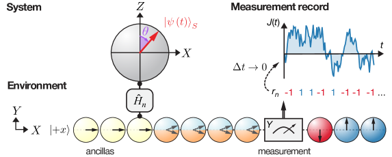
Фигура 2.3: Homodyne monitoring of a quantum bit: time-discrete model. The qubit, whose Bloch vector lies in the XZ plane, sequentially interacts with a chain of ancilla qubits, which model the environment. At the beginning of each timestep, at time $t$, the system is in a pure state, $\left|\psi\left(t\right)\right\rangle_{S}$. During the $n$-th timestep, of length $\Delta t$, the qubit interacts, subject to the Hamiltonian $\hat{H}_{n}$, with the $n$-th ancilla, prepared in $\left|+x\right\rangle$, whereafter, the Y component of its spin is projectively measured. The result of the measurement, $r_{n}$, which is either -1 or 1, is recorded and accumulated; in the continuum limit, $\Delta t\rightarrow 0$, it leads to the homodyne signal $J\left(t\right)$, a time-continuous stochastic (Weiner) process.

Time is discretized in small but finite bins of length $\Delta t$ labeled by the integer $n$, i.e., $t=n\Delta t$. During each timestep, a single spin of the environment, referred to as the ancilla, interacts with the system for time $\Delta t$, see Fig. 2.3. For simplicity, assume each spin is identically prepared in the state $\left|+x\right\rangle$. We employ the convention that the states $\left|\pm x\right\rangle$, $\left|\pm y\right\rangle$, and $\left|\pm z\right\rangle$ denote eigenstates of the Pauli X, Y, and Z operators, respectively. The interaction between the $n$-th ancilla and the system is described by the Hamiltonian

$$\hat{H}_{n}\equiv-\frac{\hbar\lambda}{2}\hat{\sigma}_{z}^{S}\otimes\hat{\sigma}_{z}^{\left(n\right)}\,,$$ (2.15)

where $\lambda$ is the strength of the interaction, $\hbar$ is Plank’s constant, and $\hat{\sigma}_{z}^{S}$ and $\hat{\sigma}_{z}^{\left(n\right)}$ denote the Pauli Z operators of the system and ancilla, respectively. For the time being, we assume that $\hat{H}_{n}$ is the only generator of system evolution, and the system Hamiltonian is zero, $\hat{H}_{S}=0$. Following the interaction, the ancilla is measured by a detector that performs a projective measurement of the ancilla spin Y component, which yields the measurement result $r_{n}=-1$ or $r_{n}=1$. The observer operating the measurement apparatus keeps track of the sum total of the measurement results, the measurement signal: $J_{t}\equiv\sqrt{\Delta t}\sum_{n^{\prime}=0}^{n}r_{n^{\prime}}$.

Note two assumptions regarding the measurement: i) the ancilla qubits are undisturbed during their flight from the system to the measurement apparatus, and ii) the measurement apparatus performs a perfect measurement, and does not add technical noise. These assumptions ensure no information is lost in the measurement, nor spurious noise is added by it; i.e., the observer has perfect access to all information there is to know in the environment, and is hence referred to as an omniscient observer.

Evolution of the composite system.

For simplicity, assume the state of the system at time $t$ is pure and its Bloch vector lies in the XZ plane; i.e., it is described by a single angle $\theta\left(t\right)$,

$$\left|\psi\left(t\right)\right\rangle_{S} =\cos\left(\frac{\theta\left(t\right)}{2}\right)\left|+z\right\rangle_{S}+\sin\left(\frac{\theta\left(t\right)}{2}\right)\left|-z\right\rangle_{S}=\begin{pmatrix}\cos\left(\frac{\theta\left(t\right)}{2}\right)\\ \sin\left(\frac{\theta\left(t\right)}{2}\right)\end{pmatrix}\,.$$ (2.16)

The state of the composite system at time $t$, consisting of the $n$-th ancilla and the system qubit, is $\left|\Psi\left(t\right)\right\rangle=\left|\psi\left(t\right)\right\rangle_{S}\otimes\left|+x\right\rangle_{n}$, and for duration $\Delta t$ evolves subject to the Hamiltonian $\hat{H}_{n}$. The total evolution is given by the propagator $\hat{U}\left(t,t+\Delta t\right)=\exp\left(-i\hat{H}_{n}\Delta t/\hbar\right)$, and the composite-system state after the interaction is

$$\left|\Psi\left(t+\Delta t\right)\right\rangle=\hat{U}\left(t,t+\Delta t\right)\left|\Psi\left(t\right)\right\rangle\,,$$ (2.17)

Anticipating the ancilla Y measurement, we express $\left|\Psi\left(t+\Delta t\right)\right\rangle$ in terms of the measurement operator eigenstates. The measurement operator on the ancilla alone is the Pauli Y operator, $\hat{\sigma}_{y}^{\left(n\right)}$, with eigenstates $\left|-y\right\rangle_{n}$ and $\left|+y\right\rangle_{n}$, in terms of which,

$$\left|\Psi\left(t+\mathrm{d}t\right)\right\rangle=\left|\tilde{\psi}_{-1}\left(t+\Delta t\right)\right\rangle_{S}\otimes\left|-y\right\rangle_{n}+\left|\tilde{\psi}_{+1}\left(t+\Delta t\right)\right\rangle_{S}\otimes\left|+y\right\rangle_{n}\,,$$ (2.18)

where the parameter $\epsilon\equiv\lambda\Delta t$ characterizes the measurement strength and the un-normalized system states $\left|\tilde{\psi}_{\pm 1}\left(t+\Delta t\right)\right\rangle_{S}$ are

$$\left|\tilde{\psi}_{\pm 1}\left(t+\Delta t\right)\right\rangle_{S}\equiv\begin{pmatrix}\cos\left(\frac{\theta\left(t\right)}{2}\right)\cos\left(\frac{\pi/2\pm\epsilon}{2}\right)\\ \sin\left(\frac{\theta\left(t\right)}{2}\right)\sin\left(\frac{\pi/2\pm\epsilon}{2}\right)\end{pmatrix}_{S}\,.$$ (2.19)

The state of the composite system following the interaction, Eq. (2.18), is not separable. The interaction has entangled the system and environment, as discussed of Sec. 2.1.3.

Projective (von Neumann) measurement of the ancilla.

The action of the measurement apparatus on the composite system is described, recalling the discussion on Pg. 2.1.3, by decomposing the measurement operator $\hat{Y}_{n}=\hat{I}\otimes\hat{\sigma}_{y}$ in terms of its eigenstate projectors, $\hat{\pi}_{\pm}\equiv\hat{I}_{S}\otimes\left(\left|\pm y\right\rangle\left\langle\pm y\right|\right)_{n}$; note, $\hat{Y}=\hat{\pi}_{+}-\hat{\pi}_{-}$. According to the von Neumann postulate, the projectors yield the probability for obtaining the results $r_{n}=-1$ and $r_{n}=1$ from the measurement,

$$\wp_{r}\left(t\right) =\left\langle\Psi\left(t+\Delta t\right)\right|\hat{\pi}_{r}\left|\Psi\left(t+\Delta t\right)\right\rangle$$

$$=\left\langle\tilde{\psi}_{r}\left(t+\Delta t\right)\middle|\tilde{\psi}_{r}\left(t+\Delta t\right)\right\rangle$$

$$=\frac{1}{2}\left(1-r_{n}\sin\left(\epsilon\right)\cos\left(\theta\left(t\right)\right)\right)\,,$$ (2.20)

as well as the state of the composite system immediately after the measurement, conditioned on the result $r_{n}$,

$$\left|\Psi_{r}\left(t+\Delta t\right)\right\rangle=\left|\tilde{\psi}_{r}\left(t+\Delta t\right)\right\rangle_{S}\left|y:=r\right\rangle_{n}/\sqrt{\wp_{r}\left(t\right)},$$ (2.21)

where $\left|y:=r\right\rangle_{n}$ denotes ancilla state $\left|+y\right\rangle_{n}$ (resp., $\left|-y\right\rangle_{n}$) for $r=1$ (resp., $r=-1$). The measurement has transformed the entanglement between the system and environment, evident in the non-separable state $\left|\Psi\left(t+\Delta t\right)\right\rangle$, Eq. (2.18), into a correlation between the pure state of the system and environment after the measurement, evident in the separable, non-entangled conditional state $\left|\Psi_{r}\left(t+\Delta t\right)\right\rangle$, Eq. (2.21). Assuming the ancilla never interacts with the system again, it is unnecessary to retain it in the description of the measurement; removing it from Eq. (2.21), we obtain the pure state of the system alone at time $t+\Delta t$:

$$\left|\psi_{r}\left(t+\Delta t\right)\right\rangle_{S} =\frac{1}{\sqrt{\wp_{r}\left(t\right)}}\left|\tilde{\psi}_{r}\left(t+\Delta t\right)\right\rangle_{S}=\begin{pmatrix}\cos\left(\frac{\theta_{r}\left(t+\mathrm{d}t\right)}{2}\right)\\ \sin\left(\frac{\theta_{r}\left(t+\mathrm{d}t\right)}{2}\right)\end{pmatrix}\,.$$ (2.22)

From the point of view of the observer, the entanglement is transformed by the measurement into a classical correlation between the result $r_{n}$ and the final conditional state of the system, $\left|\psi_{r}\left(t+\Delta t\right)\right\rangle_{S}$. Figure 2.4 summarizes the steps of the model and the conditional state update.

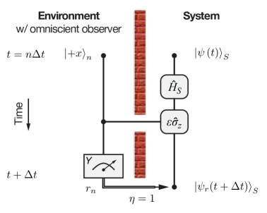
Фигура 2.4: Circuit representation of the $n$-th timestep of the quantum trajectory. At time $t=n\Delta t$, the system, described by the state $\left|\psi\left(t\right)\right\rangle_{S}$, is subjected to the system Hamiltonian $\hat{H}_{S}$ and the interaction with the $n$-th ancilla, characterized by the parameter $\epsilon$. Every ancilla is prepared in $\left|+x\right\rangle$. Following the interaction, the detector projectively measures the Y component of the ancilla spin, yielding the result $r_{n}$, which provides the information necessary to update the state of the system. In the case of the omniscient observer, characterized by unit quantum measurement efficiency, $\eta=1$, at the end of the timestep, immediately after $t+\Delta$, the system state, $\left|\psi_{r}\left(t+\Delta t\right)\right\rangle_{S}$, conditioned on the measurement result is pure. Contrast with Fig. 2.2.

Solution for the conditional state update.

To explicitly solve Eq. (2.22) for the updated angle of the qubit system conditioned on the measurement result $r_{n}$, $\theta_{r}\left(t+\Delta t\right)$, one can use Eqs. (2.20) and (2.19), following trigonometric manipulation, to obtain, without any approximations, an explicit relation (Devoret, M.H.) between the Bloch angle at the start and end of the timestep:

$$\boxed{\tan\left(\frac{\theta_{r}\left(t+\Delta t\right)}{2}\right)=\tan\left(\frac{\theta\left(t\right)}{2}\right)\tan\left(\frac{\pi/2+r_{n}\epsilon}{2}\right)\,.}$$ (2.23)

In the following section, Sec. 2.2.2, this seemingly non-linear equation is transformed into a linear equation by a hyperbolic transformation of the circular angle $\theta$, and is solved exactly. Nonetheless, for the continuum-limit discussion in Sec. 2.2.3, consider the solution of Eq. (2.23) in the limit of weak interactions, $\epsilon\ll 1$, to order $\epsilon$:

$$\mathrm{d}\theta\left(t\right)\equiv\theta\left(t+\Delta t\right)-\theta\left(t\right)\approx\epsilon r_{n}X\left(t\right)\,,$$ (2.24)

where we have defined the Bloch angle increment, $\mathrm{d}\theta\left(t\right)$, and $X\left(t\right)$ is the X component of the Bloch vector, $X\left(t\right)=\sin\left(\theta\left(t\right)\right)$.

Interpretation and remarks.

The system measurement dynamics are described in entirety by Eqs. (2.20), (2.22), and (2.24). To make the discussion more concrete, consider the particular case where the system and ancilla do not interact, $\epsilon=0$. The measurement results are completely random, $\wp_{r}=\frac{1}{2}$, uncorrelated with the system; similarly, the system state is independent of the measurement results, $r_{n}$; in fact, there is no state evolution, $\mathrm{d}\theta\left(t\right)=0$. Consider the more interesting case of weak interactions, $\epsilon\ll 1$. Measurement results are correlated with the Z component of the system Bloch vector, $\wp_{r}=\frac{1}{2}\left(1-\epsilon r_{n}Z\left(t\right)\right)$, where $Z\left(t\right)=\cos\left(\theta\left(t\right)\right)$. Nonetheless, due to $\epsilon\ll 1$, the two measurement results still occur with nearly equal probability, and the record consists of random noise, but with a slight bias that correlates it with $Z$. Thus, the value of $Z$ can be obtained from the instantaneous average of the measurement results, $\textrm{E}\left[r_{n}\right]=-\epsilon Z$. In time, from the point of view of the observer, a long sequence of measurements gradually results in the complete measurement of $Z$, obtained from the noisy measurement record. A peculiar feature of the weak interaction regime, $\epsilon\ll 1$, is that amplitude of the noise is essentially constant for all measurement strengths, its variance is $\mathrm{Var}\left[r_{n}\right]=1-\left(\epsilon Z\right)^{2}\approx 1$. This origin of the randomness can be interpreted to be quantum in nature, since the system and environment are in pure states at all times. Specifically, it is due to the incompatibility (orthogonality) between the initial state of the ancilla, $\left|+x\right\rangle_{n}$, and the eigenstates, $\left|\pm y\right\rangle_{n}$, of the measurement observable.

The random measurement result, $r_{n}$, is correlated with a small ‘‘kick’’ on the state of the system, described by Eq. (2.24). Conditioned on the result $r_{n}=1$ (resp., $r_{n}=-1$) the system experiences a downward (resp., upward) kick corresponding to the circular increment $\mathrm{d}\theta\left(t\right)=\epsilon r_{n}\mathrm{sgn}\left(X\left(t\right)\right)\sqrt{1-Z\left(t\right)}$, whose magnitude is largest for $Z=0$, but vanishing in the limit where $Z$ approaches $\pm 1$; the sign function is denoted $\mathrm{sgn}$. This state-dependent nature of the back-action kicks leads to the eventual projection of the state onto one of the eigenstate of the system observable, $\hat{\sigma}_{z}$, as discussed in Sec. 2.2.2.

The form of the backaction depends on the ancilla quantity being measured by the apparatus; for example, a measurement of a quadrature other than the ancilla $Y$ quadrature yields a different form of the measurement backaction. More generally, we emphasize that no matter what ancilla quantity is measured, so long as the measurement is projective and complete knowledge about the ancilla is obtained, the ancilla is collapsed onto a single unique state. From this, it follows that the system cannot be entangled with the ancilla and for this reason the system is left in a pure state.

Generalized measurements.

By introducing an ancilla that interacts unitarily with the system and is subsequently measured, we obtained evolution equations for the pure state of the quantum system conditioned on the measurement result $r_{n}$, and could otherwise disregard the ancilla in the measurement description. The ancilla scheme realizes an indirect measurement of the system, which gradually obtains information about the system and disturbs it in a manner that is indescribable with the von Neumann formulation, summarized by Eqs. (2.13) and (2.14). The example of this section belongs to a more general class of measurements, referred to as generalized measurements. A powerful theorem by Neumark, see Sec. 9-6 of Ref. Peres (2002), proved that any generalized measurement can be formulated essentially according to the scheme presented so far, where an auxiliary quantum system is introduced, it interacts unitarily with the system, and is subsequently projectively measured, in the traditional von Neumann sense. The effect of the generalized measurement on the system can be completely described by system operators, denoted $\hat{M}_{r}$, that are not in general Hermitian. For our example, the measurement operator, $\hat{M}_{r}$, follows directly from Eq. (2.21),

$$\hat{M}_{r}\left(t\right)=\prescript{}{n}{\left\langle y:=r\middle|\hat{U}\left(t,t+\Delta t\right)\middle|+x\right\rangle_{n}}$$ (2.25)

Note that $\left|+x\right\rangle_{n}$ is the initial ancilla state for the $n$-th timestep, while $\left|y:=r\right\rangle_{n}$ is the final ancilla state, follwing the projective measurement, while $\hat{U}$ is the composite system propagator. Since $\hat{M}_{r}$ in Eq. (2.25) is not Hermitian, it does not belong to the traditional notion of an ’observable’, and the outcomes $r_{n}$ are not the eigenvalues of $\hat{M}_{r}$, but serve merely as labels. The measurement operators $\hat{M}_{1}$ and $\hat{M}_{-1}$, which are non-orthogonal ($\hat{M}_{1}\hat{M}_{-1}\neq 0$) link the system state with the set of measurement probabilities $\wp_{r}$, and formally, their operator set, $\left\{\hat{M}_{r}^{\dagger}\hat{M}_{r}:r\right\}$, constitutes a positive-operator-valued measure (POVM) on the space of results, see Sec. 2.2.6 of Ref. Nielsen and Chuang (2010). In general, the measurement operators generalize von Neumann’s postulate in the following way:

$$\wp_{r}\left(t\right)= \textrm{Tr}\left[\hat{M}_{r}\rho\hat{M}_{r}^{\dagger}\right]\,,$$ (2.26)

$$\rho_{r}\left(t+\Delta t\right)= \hat{M}_{r}\rho\left(t\right)\hat{M}_{r}^{\dagger}/\wp_{r}\left(t\right)\,,$$ (2.27)

where $\wp_{r}\left(t\right)$ is the probability to obtain the measurement outcome $r$ and $\rho_{r}\left(t+\Delta t\right)$ is the state of the system immediately after the measurement, conditioned on the result $r$. Note that technically, the generalized projection postulate does not introduce anything fundamentally new beyond von Neumann’s postulate, since it follows from Neumark’s theorem that considering a larger quantum system with projective (von Neumann) measurements and unitary operations is completely equivalent.

2.2.2 Geometric representation of a continuous measurement: random walk on a hyperbola

In this subsection, we present a geometric representation of the measurement dynamics. Section 2.1.3 presented the geometric representation of the qubit state as a point on the Bloch sphere, with coordinates $X$, $Y$, and $Z$, or for a pure state, as a point on the surface of the sphere, parameterized by the angles $\theta$ and $\phi$, Eq. (2.11). For our qubit example, $Y=0$ by assumption, hence its pure state, $\left|\psi\right\rangle_{S}$, can be represented on the Bloch circle, see Fig. 2.5a, parametrized by a single circular angle $\theta$: $X=\sin\left(\theta\right)$ and $Z=\cos\left(\theta\right)$. This geometric representation is particularly well suited to describing unitary operations, which describe rotations in Hilbert space. For concreteness, consider the state evolution subject to the Rabi Hamiltonian $\hat{H}_{S}=\frac{1}{2}\hbar\omega\hat{\sigma}_{y}$, where, without assumptions on the timestep, $\Delta t$, the effect of the propagator $U\left(t,t+\Delta t\right)=\exp\left(-i\hat{H}_{S}\Delta t/\hbar\right)$ on the state is given by the simple linear equation:

$$\theta\left(t+\Delta t\right)-\theta\left(t\right)=\omega\Delta t\,.$$ (2.28)

The complexity of Eq. (2.23) indicates that the circular representation is not well suited to describe the evolution due to the measurement. Rather, we show that a natural representation for measurement dynamics is a hyperbolic one.

Hyperbolic representation.

We map the Bloch circle onto the standard hyperbola according to the equation $Z=\cos\left(\theta\right)=\tanh\zeta$, where $\zeta$ is the hyperbolic angle, the analogue of the circular angle $\theta$, see Fig. 2.5a. In terms of the hyperbolic representation, without any approximations, Eq. (2.23) is transformed into a simple linear equation, analogous to that of Eq. (2.28),

$$\zeta_{r}\left(t+\Delta t\right)-\zeta\left(t\right)=-r_{n}\xi\,,$$ (2.29)

where $\zeta_{r}\left(t+\Delta t\right)$ is the hyperbolic angle of the system after the measurement, conditioned on the result $r_{n}$, $\zeta\left(t\right)$ is the hyperbolic angle before the interaction with the ancilla, and $\xi$ is the hyperbolic increment, $\tanh\left(\xi\right)=\sin\left(\epsilon\right)$. In view of the Eq. (2.29), the measurement backaction kicks are understood as hyperbolic rotations of a definite amplitude $\xi$, but random orientation $r_{n}$. By iterating the calculation of Eq. (2.29) $N$ times, one can obtain the stochastic path taken by the qubit state, its quantum trajectory, which, understood in terms of the stochastic difference equation $\mathrm{d}\zeta_{r}\left(t\right)\equiv\zeta_{r}\left(t+\Delta t\right)-\zeta\left(t\right)=-r_{n}\xi$, is a random walk on a hyperbola.

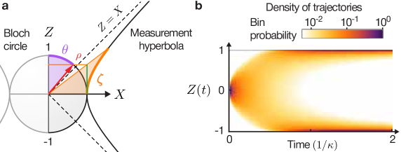
Фигура 2.5: Random walk on the measurement hyperbola. a, Circular and hyperbolic geometric representations of the pure qubit state, $\rho$, parametrized by the circular and hyperbolic angles $\theta$ and $\zeta$, respectively, obeying $\cos\left(\theta\right)=\tanh\zeta$. The circle depicts a slice though the XZ plane of the Bloch sphere, which is well-suited to represent unitary dynamics. The random walk of $\zeta$ due to the measurement takes place on the unit hyperbola, with asymptotes defined by the lines $Z=\pm X$. b, Histogram of quantum trajectory densities obtained from simulations of the flying-spin model. All trajectories (not shown here) begin with the initial state defined by the Bloch coordinates $X\left(0\right)=1$ and $Z\left(0\right)=0$. The time axis is scaled in units of the measurement rate, $\kappa$.

The circular and hyperbolic coordinate transformations together with Eqs. (2.28) and (2.29) can be employed to construct a finite-difference numerical scheme to calculate the quantum trajectory of the qubit subject to homodyne monitoring. Notably, since the difference equations were derived without approximations, especially with regard to the size of $\Delta t$, they guarantee a physical system state for all parameters and at all time, features which offer some practical advantages for numerical simulations. In the following subsection, Sec. 2.2.3, we construct the continuum limit of the model and formally derive the differential equations for the quantum trajectory of the qubit.

2.2.3 Continuum limit: Wiener noise and stochastic calculus

In this section, we take the appropriate limit in which the measurement becomes continuous. In this limit, the interaction time, $\Delta t$, becomes infinitely small while the measurement strength, $\lambda$, becomes infinitely large. Since each short sequence of individual measurements carries an infinitesimal amount of information in this limit, we coarse-grain the measurement record in the following way. The evolution up to time $t$ is divided in $m$ intervals of total duration $\mathrm{d}t$, while each of these intervals is further subdivided in $l$ yet smaller intervals, each of duration $\Delta t$; i.e., $t=n\Delta t=ml\Delta t$ and $\mathrm{d}t=l\Delta t$. The interaction amplitude, $\lambda$, is chosen to be $\lambda=\sqrt{\kappa/\Delta t}$, where $\kappa$ denotes the interaction rate. Subject to appropriate scaling, by a factor $\sqrt{\Delta t}$, the sum of all measurement results up to time $t$ is the measurement signal $J_{t}=\sqrt{\Delta t}\sum_{m^{\prime}=0}^{m}\sum_{l^{\prime}=0}^{l}r_{m^{\prime}l^{\prime}}$. During a time interval $\mathrm{d}t$, beginning at $t=ml\Delta t$ and ending at $t^{\prime}=\left(m+1\right)l\Delta t$, the signal changes by

$$\mathrm{d}J_{t}=J_{\left(m+1\right)l\Delta t}-J_{ml\Delta t}=\sqrt{\Delta t}\sum_{k=ml}^{\left(m+1\right)l}r_{k}\>.$$ (2.30)

Equation (2.30) is known as a stochastic difference equation, because the difference increment in the variable $J_{t}$ is a random variable. Assuming the state of the system does not appreciably change over the time interval $\mathrm{d}t$, the measurement results, $r_{k}$, are independent and identically distributed binary random variables described by the probability function $\wp\left[r_{k}\right]=\frac{1}{2}\left(1-\epsilon r_{k}Z\left(t\right)\right),$ recall Eq. (2.20), where $\epsilon=\sqrt{\kappa\Delta t}$. It follows that the mean and variance of the measurement increment are

$$\textrm{E}\left[\mathrm{d}J_{t}\right] =l\sqrt{\Delta t}\textrm{E}\left[r_{k}\right]=-\sqrt{\kappa}Z\left(t\right)\mathrm{d}t\,,$$ (2.31)

$$\mathrm{Var}\left[\mathrm{d}J_{t}\right]= l\Delta t\mathrm{Var}\left[r_{k}\right]\approx\mathrm{d}t\,,$$ (2.32)

respectively, while, according to the central limit theorem, all higher-order cumulants of the probability distribution for $\mathrm{d}J_{t}$ vanish in the limit of large $l$. Working in this limit, and employing Eqs. (2.31) and (2.32), the stochastic difference equation, Eq. (2.30), can be taken to the continuum limit,

$$\boxed{\mathrm{d}J\left(t\right)=-\sqrt{\kappa}Z\left(t\right)\mathrm{d}t+\mathrm{d}W\left(t\right)\,},$$ (2.33)

where the infinitesimal term $\mathrm{d}W\left(t\right)$ represents Gaussian white noise, and is known as the Wiener increment. It obeys the following canonical relations and probability density:

$$\textrm{E}\left[\mathrm{d}W\left(t\right)\right] =0\,, \mathrm{d}W\left(t\right)\mathrm{d}t =0\,,$$ (2.34)

$$\textrm{E}\left[\mathrm{d}W\left(t\right)^{2}\right] =\mathrm{d}t\,, \wp\left(\mathrm{d}W\right) =\frac{\exp\left(-\mathrm{d}W^{2}/(2\mathrm{d}t)\right)}{\sqrt{2\pi\mathrm{d}t}}\,.$$ (2.35)

Stochastic calculus.

Equation (2.33) is known as a stochastic differential equation (SDE) because the infinitesimal differential is not completely determined, but is a random variable. Notably, in obtaining this equation, we took the value of the function $Z\left(t\right)$ at the beginning of the timestep $\mathrm{d}t$. In general, because the stochastic noise is not smooth and not differentiable if we had taken the value of the function at the end of the time-interval $\mathrm{d}t$ we would have obtained a different form of the SDE. By taking the value of the function at the beginning of the timestep, the SDE we obtained is said to be in Itô form; otherwise, it would have been in Stratonovich form. The two forms are not equivalent in a straightforward manner, but for our purposes, it will suffice to only consider the Itô form; see Chapter 3 of Ref. Jacobs (2010) for an in-depth discussion. From Eqs. (2.34) and (2.35) it follows that the SDE solution only depends on terms proportional to $\mathrm{d}t,$ $\mathrm{d}W,$ and $\mathrm{d}W^{2},$ while all other terms of the form $\mathrm{d}t^{p}\mathrm{d}W^{q}$ are vanishing. Importantly, in an unusual departure from the rules of differential calculus, in the continuum limit, one can set $\mathrm{d}W^{2}=\mathrm{d}t$, a result known as Itô’s rule. We note that $\mathrm{d}W\left(t\right)$ is an idealized Gaussian noise process in that it has a perfect delta function correlation in time, which implies its Markovianity, but also that it has a white noise power spectral density, non-zero for all frequencies.

Itô SDE for the Bloch vector.

In our example, the Bloch vector of the qubit can be parameterized by its Z component, $\vec{S}\left(t\right)=\left(\sqrt{1-Z\left(t\right)^{2}},0,Z\left(t\right)\right)^{\intercal}$. Thus, it suffices to derive an SDE for $Z\left(t\right)$, which is obtained from the system state, $\left|\psi_{J}\left(t\right)\right\rangle$, conditioned on the measurement signal $J\left(t\right)$ by taking the expectation value of $\hat{\sigma}_{z}$, $Z\left(t\right)=\left\langle\psi_{J}\left(t\right)\middle|\hat{\sigma}_{z}\middle|\psi_{J}\left(t\right)\right\rangle$. The SDE is derived by first Taylor expanding $Z\left(t\right)=\cos\left(\theta\left(t\right)\right)$ to first order in $\mathrm{d}t$, $\mathrm{d}Z\left(t\right)\approx-\sqrt{1-Z\left(t\right)^{2}}\mathrm{d}\theta\left(t\right)-\frac{1}{2}Z\left(t\right)\mathrm{d}\theta\left(t\right)^{2}$, where we have retained terms to second order in $\mathrm{d}\theta\left(t\right)$. This is necessary because $\mathrm{d}\theta\left(t\right)$, recalling Eq. (2.24), is proportional to $\mathrm{d}W$, and $\mathrm{d}W^{2}=\mathrm{d}t$. By summing $l$ times over the difference equation and performing the same coarse graining employed to arrive at Eq. (2.33), we arrive at the Itô form of the SDE for the Z component of the Bloch vector of a qubit subject to heterodyne monitoring of $\hat{\sigma}_{z}$,

$$\boxed{\mathrm{d}Z\left(t\right)=-\sqrt{\kappa}\left(1-Z\left(t\right)^{2}\right)\mathrm{d}W\left(t\right)\,.}$$ (2.36)

Equation (2.36) is a non-linear diffusion equation with a state-dependent diffusion coefficient, $D\left(Z\right)=\kappa\left(1-Z^{2}\right)^{2}$, which is maximized for $Z\left(t\right)=0$, but approaches zero for $Z=\pm 1$. Mathematically, it is for this reason, that in the limit $t\rightarrow\infty$, the system tends to one of the pointer states ($Z=\pm 1$) of the measurement, where diffusion vanishes, and states cluster.

2.3 Quantum trajectory theory

The preceding sections introduced the general background required to develop quantum trajectory theory. With the aid of specific examples, important overriding themes were highlighted, which will carry us forward in this section, and play a key role in understanding photon-counting, homodyne, and heterodyne measurements.

2.3.1 Photodetection

Photodetection is the minimal time-continuous measurement scheme — at each moment in time, the detector records one of only two possible results: $r=0$ (‘‘no-click’’) or $r=1$ (‘‘click’’). As discussed in Sec. 2.2, the measurement result communicates some knowledge about the system state and the unavoidable disturbance caused to it by the measurement itself. The information gain as well as the action of the disturbance are encoded in the measurement operators, $\hat{M}_{r}$, recall Eq. (2.25). These operators, also known as Kraus operators, generalize unitary evolution due to a system Hamiltonian, $\hat{H}$, so as to include the effect of the measurement process. Microscopically, the measurement operators, $\hat{M}_{r}$, can be understood to describe the unitary interaction between the system and another, auxiliary one, which is subsequently measured by a von Neumann measurement apparatus, see discussion on Neumark’s theorem in Sec. 2.2. In this section, we will only concern ourselves with the system evolution subject to measurement, and will make no further reference to the auxiliary system, other than to specify the system operator $\hat{c}$ that couples the two. The minimal set of infinitesimal measurement operators, which corresponding to the no-click ($r=0$) and click ($r=1$) evolution, are

$$\hat{M}_{0}\left(\mathrm{d}t\right) =\hat{1}-\left(\frac{1}{2}\hat{c}^{\dagger}\hat{c}+i\hat{H}\right)\mathrm{d}t\,,$$ (2.37)

$$\hat{M}_{1}\left(\mathrm{d}t\right) =\sqrt{dt}\hat{c}\,,$$ (2.38)

in units where $\hbar=1$. One can verify that $\hat{M}_{0}\left(\mathrm{d}t\right)$ and $\hat{M}_{1}\left(\mathrm{d}t\right)$ form a positive-operator-valued measure (POVM) on the space of results. Hence, they form a resolution of the identity, $\hat{M}_{0}^{\dagger}\left(\mathrm{d}t\right)\hat{M}_{0}\left(\mathrm{d}t\right)+\hat{M}_{1}^{\dagger}\left(\mathrm{d}t\right)\hat{M}_{1}\left(\mathrm{d}t\right)=\hat{1}+\mathcal{O}\left(\mathrm{d}t^{2}\right)$, guaranteeing that the law of total probability is satisfied, i.e., a measurement yields an outcome with probability 1. The probability for a specific outcome, $r=0$ or $r=1$, is is given by the generalized measurement postulate, Eq. (2.26), $\wp_{r}\left(\mathrm{d}t\right)=\left\langle\hat{M}_{r}^{\dagger}\left(\mathrm{d}t\right)\hat{M}_{r}\left(\mathrm{d}t\right)\right\rangle$,

$$\wp_{0}\left(\mathrm{d}t\right) =1-\mathrm{d}t\left\langle\hat{c}^{\dagger}\hat{c}\right\rangle+\mathcal{O}\left(\mathrm{d}t^{2}\right)\,,$$ (2.39)

$$\wp_{1}\left(\mathrm{d}t\right) =\mathrm{d}t\left\langle\hat{c}^{\dagger}\hat{c}\right\rangle\,.$$ (2.40)

We define the time-continuous photodetection measurement record to be the number of photodetections up to time $t$, denoted $N\left(t\right)$. It follows that the infinitesimal measurement increment, denoted $\mathrm{d}N\left(t\right)$, is a point-process, also known as the Poisson process, defined by

$$\mathrm{d}N\left(t\right)^{2} =\mathrm{d}N\left(t\right)\,,$$ (2.41)

$$\textrm{E}\left[\mathrm{d}N\left(t\right)\right] =\wp_{1}\left(\mathrm{d}t\right)\,,$$ (2.42)

where $\textrm{E}\left[\cdot\right]$ denotes the expectation value in the classical sense, see Sec. 2.1.1. In the continuum limit, the detector photocurrent, $I\left(t\right)=\mathrm{d}N\left(t\right)/\mathrm{d}t$, consists of a series of Dirac $\delta$-functions at the times of the clicks.

Stochastic master equation (SME) for ideal photodetection.

Ideal photodetection is the limit where the photodetector collects the entirety of the system output field and adds no technical noise, i.e., the quantum measurement efficiency is one, $\eta=1$. According to the generalized projection postulate, Eq. (2.27), the state of the system after a measurement at time $t$ conditioned on the measurement result $r=0$ or $r=1$ is

$$\rho_{r}\left(t+\mathrm{d}t\right)=\frac{\hat{M}_{r}\left(\mathrm{d}t\right)\rho\left(t\right)\hat{M}_{r}^{\dagger}\left(\mathrm{d}t\right)}{\wp_{r}\left(\mathrm{d}t\right)}\,.$$ (2.43)

In the continuum limit, where the instantaneous measurement outcome is the photocurrent $I\left(t\right),$ the two possible states, $\rho_{0}\left(t+\mathrm{d}t\right)$ and $\rho_{1}\left(t+\mathrm{d}t\right)$, can be combined in a single stochastic differential equation (SDE) for the posterior system state $\rho_{I}\left(t+\mathrm{d}t\right)$ conditioned on $I\left(t\right)$, resulting in the state differential, in Itô form,

$$\mathrm{d}\rho_{I}\left(t\right) =\rho_{I}\left(t+\mathrm{d}t\right)-\rho_{I}\left(t\right)$$ (2.44)

$$=\mathrm{d}N\left(t\right)\left(\rho_{1}\left(t+\mathrm{d}t\right)-\hat{1}\right)+\left(1-\mathrm{d}N\left(t\right)\right)\left(\rho_{0}\left(t+\mathrm{d}t\right)-\hat{1}\right)\,,$$ (2.45)

which can be simplified by Taylor expanding the denominator of $\rho_{0}\left(t+\mathrm{d}t\right)$, retaining terms to order $\mathrm{d}t$, and employing the stochastic calculus rule

$$\mathrm{d}N\left(t\right)\mathrm{d}t=0\,$$ (2.46)

in order to obtain the stochastic master equation (SME) for photodetection, in the Schrödinger picture and in Itô form,

$$\boxed{\mathrm{d}\rho_{I}\left(t\right)=\left(\mathrm{d}N\left(t\right)\mathcal{G}\left[\hat{c}\right]+\mathrm{d}t\mathcal{H}\left[\hat{H}_{\mathrm{eff}}\right]\right)\rho_{I}\left(t\right)\,,}$$ (2.47)

where the superoperators $\mathcal{G}\left[\hat{c}\right]\rho$ and $\mathcal{H}\left[\hat{c}\right]\rho$ are defined by

$$\mathcal{G}\left[\hat{c}\right]\rho\equiv \frac{\hat{c}^{\dagger}\rho\hat{c}}{\textrm{Tr}\left[\hat{c}^{\dagger}\rho\hat{c}\right]}-\rho\,,$$ (2.48)

$$\mathcal{H}\left[\hat{c}\right]\rho\equiv \hat{c}\rho+\rho\hat{c}^{\dagger}-\textrm{Tr}\left[\hat{c}\rho+\rho\hat{c}^{\dagger}\right]\rho$$ (2.49)

$$= \left(\hat{c}-\left\langle\hat{c}\right\rangle\right)\rho+\rho\left(\hat{c}^{\dagger}-\left\langle\hat{c}^{\dagger}\right\rangle\right)\,,$$ (2.50)

The superoperator $\mathcal{G}$ results in point-like discontinuous state evolution, while $\mathcal{H}$ results in smooth, continuous, but non-unitary evolution generated by the effective non-Hermitian Hamiltonian

$$\hat{H}_{\text{eff}}\equiv\hat{H}-i\frac{1}{2}\hat{c}^{\dagger}\hat{c}\,.$$ (2.51)

Notably, the trace terms in Eqs. (2.48) and (2.49) make the photodetection SME, Eq. (2.47), nonlinear in the state density, $\rho_{I}$. The origin of the trace term in $\mathcal{H}$, namely $\textrm{Tr}\left[\hat{c}\rho+\rho\hat{c}^{\dagger}\right]$, is the Taylor expansion of the denominator of Eq. (2.43), which gives the no-click probability, $\wp_{0}\left(\mathrm{d}t\right)$. As discussed in Sec. 2.2, the role of this term is to preserve the state density trace for all time, $\textrm{Tr}\left[\rho_{I}\left(t\right)\right]=1$. The solution of the SME is a stochastic path taken by the conditional state over time, known as a quantum trajectory, a term coined in Ref. Carmichael (1993).

Stochastic Schrödinger equation (SSE) for photodetection.

For a system in a pure state, $\rho_{I}\left(t\right)=\left|\psi_{I}\left(t\right)\right\rangle\left\langle\psi_{I}\left(t\right)\right|$, the SME, Eq. (2.47), preserves the purity of the state for all times. It follows that the state evolution is described by a type of Schrödinger equation, known as the stochastic Schrödinger equation (SSE),

$$\boxed{\mathrm{d}\left|\psi_{I}\left(t\right)\right\rangle=\left[\mathrm{d}t\left(\frac{\left\langle\hat{c}^{\dagger}\hat{c}\right\rangle\left(t\right)}{2}-\frac{\hat{c}^{\dagger}\hat{c}}{2}-i\hat{H}\right)+\mathrm{d}N\left(t\right)\left(\frac{\hat{c}}{\sqrt{\left\langle\hat{c}^{\dagger}\hat{c}\right\rangle\left(t\right)}}-\hat{1}\right)\right]\left|\psi_{I}\left(t\right)\right\rangle\,,}$$ (2.52)

which is nonlinear in the state $\left|\psi_{I}\left(t\right)\right\rangle$. The non-linear terms contain the expectation value $\left\langle\hat{c}^{\dagger}\hat{c}\right\rangle\left(t\right)=\frac{1}{2}\left\langle\psi_{I}\left(t\right)\middle|\hat{c}^{\dagger}\hat{c}\middle|\psi_{I}\left(t\right)\right\rangle$, which gives the click probability $\wp_{1}$, see Eq. (2.40). Because these non-linear terms render analytic treatment of the equations particularly difficult in general, a linear description of the state evolution is desired, and can be accomplished as described next. The term $\frac{1}{2}\mathrm{d}t\left\langle\hat{c}^{\dagger}\hat{c}\right\rangle\left(t\right)\left|\psi_{I}\left(t\right)\right\rangle$, which updates the observer’s state-of-knowledge in a non-linear way, mathematically, ensures the proper normalization of $\left|\psi_{I}\left(t\right)\right\rangle$ for all times; however, normalization need not be enforced for each infinitesimal timestep $\mathrm{d}t$. Instead, it can ‘‘manually’’ be enforced for the no-click periods, $I\left(t\right)=0$, by first first solving for the un-normalized system state, denoted with a tilde, $\left|\tilde{\psi}_{I=0}\left(t\right)\right\rangle$, then normalizing it, $\left|\psi_{I=0}\left(t\right)\right\rangle=\left|\tilde{\psi}_{I=0}\left(t\right)\right\rangle/\left\langle\tilde{\psi}_{I=0}\left(t\right)\middle|\tilde{\psi}_{I=0}\left(t\right)\right\rangle$, where the effective Schrödinger equation for $\left|\tilde{\psi}_{I=0}\left(t\right)\right\rangle$ is

$$\boxed{i\frac{\mathrm{d}}{\mathrm{d}t}\left|\tilde{\psi}_{I=0}\left(t\right)\right\rangle=\hat{H}_{\mathrm{eff}}\left|\tilde{\psi}_{I=0}\left(t\right)\right\rangle\,,}$$ (2.53)

where $\hat{H}_{\mathrm{eff}}$ is the non-Hermitian Hamiltonian, Eq. (2.51). Since Eq. (2.53) is linear, it is generally easier to solve for the time-dynamics. Calculation of system averages still requires normalizing $\left|\tilde{\psi}_{I=0}\left(t\right)\right\rangle$ by its the state norm, $\left\langle\tilde{\psi}_{I}\left(t\right)\middle|\tilde{\psi}_{I}\left(t\right)\right\rangle$, which gives the probability of no-clicks occurring for duration $t$. We remark that Eq. (2.53) corresponds to tracking the sub-ensemble of quantum trajectories that contain no clicks, or mathematically, to the repetitive application of the measurement operator $\hat{M}_{0}$; hence, in general, in the limit $t\rightarrow\infty$, it leads to the decay of the norm to zero.

Unconditioned evolution: master equation for photodetection.

By averaging over all possible evolutions due to all measurement outcomes at each instant, one can obtain the unconditioned evolution of the quantum state, denoted $\rho\left(t+\mathrm{d}t\right)$, from Eq. (2.47). Simplifying the average, $\rho\left(t+\mathrm{d}t\right)=\sum_{r}\wp_{r}\rho_{r}\left(t+\mathrm{d}t\right)$,

$$\rho\left(t+\mathrm{d}t\right) =\hat{M}_{0}\left(\mathrm{d}t\right)\rho\hat{M}_{0}^{\dagger}\left(\mathrm{d}t\right)+\hat{M}_{1}\left(\mathrm{d}t\right)\rho\hat{M}_{1}^{\dagger}\left(\mathrm{d}t\right)$$ (2.54)

$$=\rho\left(t\right)-i\left[\hat{H},\rho\left(t\right)\right]\mathrm{d}t+\mathcal{D}\left[\hat{c}\right]\rho\left(t\right)\mathrm{d}t\,,$$ (2.55)

where the superoperator $\mathcal{D}$ is defined to be

$$\mathcal{D}\left[\hat{c}\right]\rho\equiv\hat{c}\rho\hat{c}^{\dagger}-\frac{1}{2}\left\{\hat{c},\rho\right\}_{+}\,.$$ (2.56)

Eq. (2.55) for the unconditioned state evolution is known as the master equation, in Lindblad form (Lindblad, 1976). Unlike the SME, it is linear in the state density, $\rho$, and yields deterministic state evolution, since there are no stochastic increments, $\mathrm{d}N$ or $\mathrm{d}W$. Notably, the master equation is very general and makes no reference to photodetection, other than specifying the system operator $\hat{c}$ subject to detection, although it does not specify how. As will be evident from the following section, the same master equation is obtained for heterodyne detection of $\hat{c}$, see Sec. 2.3.2. The two SMEs corresponding to the same master equation are known as unravellings of it. We note that the unravellings of the master equation are not unique.

Imperfect detection.

Imperfect conditions limit the observer’s access to information regarding the system and generally result in excess noise. The effect of imperfections can be modeled by considering an ideal photodetector that is, however, sensitive to only a fraction $\eta$ of the system output field. This fraction, known as the quantum measurement efficiency, is a real number between zero and one, $0\leq\eta\leq 1$. Because of the loss of information due to imperfect detection, over time, the system state will, in general, become mixed, with purity less than one, $0\leq\textrm{Tr}\left[\rho^{2}\right]<1$. To account for the imperfections, SME, Eq. (2.47), is be modified in the following way, see Sec. 4.8.1 of Ref. Wiseman and Milburn (2010):

$$\boxed{\mathrm{d}\rho_{I}\left(t\right)=\left(\mathrm{d}N\left(t\right)\mathcal{G}\left[\sqrt{\eta}\hat{c}\right]+\mathrm{d}t\mathcal{H}\left[-i\hat{H}-\eta\frac{1}{2}\hat{c}^{\dagger}\hat{c}\right]+\mathrm{d}t\left(1-\eta\right)\mathcal{D}\left[\hat{c}\right]\right)\rho_{I}\left(t\right)\,,}$$ (2.57)

where the jump probability for each timestep is obtained by also replacing $\hat{c}$ with $\sqrt{\eta}\hat{c}$ in Eq. (2.42), $\textrm{E}\left[\mathrm{d}N\left(t\right)\right]=\eta\textrm{Tr}\left[\hat{c}^{\dagger}\hat{c}\rho\right]\mathrm{d}t$. Considering the two limits $\eta\rightarrow 0$ and $\eta\rightarrow 1$, one can associate the Lindblad superoperator $\mathcal{D}$ with information loss, and $\mathcal{H}$ and $\mathcal{G}$ with information gain due to the measurement.

2.3.2 Homodyne and heterodyne detection

The measurements described so far are not sensitive to the phase of the system output field, but only its amplitude. In the following, we describe dyne measurements, homodyne or heterodyne, which provide information about the phase and a qualitatively different (diffusive) trajectory unraveling.

Physical implementation.

Dyne detection is realized by mixing the system output signal with a local-oscillator (LO) tone, see Fig. 2.6. For a system carrier frequency, conventionally termed the radio frequency (RF), $\omega_{\mathrm{RF}}$ and LO frequency $\omega_{\mathrm{LO}}$, the lower sideband of the mixed-signal is at intermediate frequency (IF), $\omega_{\mathrm{IF}}=\omega_{\mathrm{LO}}-\omega_{\mathrm{RF}}$. In homodyne detection, the LO is tuned in resonance with the system carrier, resulting in a direct-current (DC) IF signal, $\omega_{\mathrm{IF}}=0$, proportional to a quadrate of the RF signal that depends on the LO phase. The IF signal is typically sampled and digitally processed. On the other hand, in heterodyne detection, the LO frequency is significantly detuned from the RF, $\omega_{\mathrm{IF}}\gg 0$, resulting in a an oscillatory IF signal, which is demodulated to extract the information-bearing in-quadrature (I) and out-of-quadrature (Q) components. Note that the heterodyne measurement record consists of a series of not one but two values, I and Q. Heterodyne detection is equivalent to two concurrent homodyne detections with LO phases $90^{\circ}$ apart.

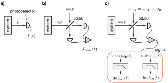
Фигура 2.6: Schematic representations of a (a) photo, (b) homodyne, and (c) heterodyne detection schemes. a, The system output field, proportional to the system coupling operator $\hat{c}$, is directly monitored with a photodetector, whose photocurrent $I\left(t\right)$ is the measurement record. b, Optical balanced homodyne detection: system output field, assumed with carrier frequency $\omega_{\mathrm{RF}}$, is interfered on a 50:50 beam splitter with a strong local oscillator (LO) tone at the carrier frequency, $\omega_{\mathrm{LO}}=\omega_{\mathrm{RF}}$. The measurement record, $J_{\mathrm{hom}}\left(t\right)$, is obtained from the difference of the photodetector currents on each output arm of the beamsplitter. c, Balanced heterodyne detection scheme (with digital demodulation): LO frequency is detuned by an intermediate frequency value, $\omega_{\mathrm{IF}},$ where $\omega_{\mathrm{IF}}\ll\omega_{\mathrm{RF}},\omega_{\mathrm{LO}}$. The difference of the photodetector currents of each arm, which oscillates at $\omega_{\mathrm{IF}}$, is digitally demodulated to obtain the in-phase [out-of-phase] quadrature $\mathrm{Re}J_{\mathrm{het}}\left(t\right)$ [$\mathrm{Im}J_{\mathrm{het}}\left(t\right)$] by digitally mixing the signal with a reference one, $\cos\left(\omega_{\mathrm{IF}}t\right)$ [$\sin\left(\omega_{\mathrm{IF}}t\right)$], and low-pass filtering the output to reject tones above $\omega_{\mathrm{IF}}$. Digital panel schematic inspired by Ref. (Campagne-Ibarcq et al., 2016b).

Homodyne measurement record.

The homodyne measurement signal is mathematically described by a function, $J_{\mathrm{hom}}\left(t\right)$, that is real and continuous everywhere but differentiable nowhere, see Sec. 2.2.3. The measurement signal gradually reveals information about a system operator of the form $\hat{c}+\hat{c}^{\dagger}$, where $\hat{c}$ is the operator coupled to the measurement apparatus, which for the example of Sec. 2.2.3 is $\hat{c}=-\frac{\sqrt{\kappa}}{2}\hat{\sigma}_{z}$. In Itô form, the measurement increment is

$$\mathrm{d}J_{\mathrm{hom}}\left(t\right)=\left\langle\hat{c}+\hat{c}^{\dagger}\right\rangle\left(t\right)\mathrm{d}t+\mathrm{d}W\left(t\right)\,,$$ (2.58)

where $\mathrm{d}W\left(t\right)$ is the stochastic Wiener increment satisfying the canonical relations given in Eqs. (2.34) and (2.35).

Heterodyne measurement record.

The heterodyne measurement signal consists of two functions: the in-phase, $J_{I}\left(t\right)$, and out-of-phase, $J_{Q}\left(t\right)$, quadrature functions, which can be combined in a single complex function, $J_{\mathrm{het}}\left(t\right)\equiv\frac{1}{2}\left(J_{I}\left(t\right)+iJ_{Q}\left(t\right)\right)$, continuous everywhere but differentiable nowhere. In heterodyne detection, $J_{\mathrm{het}}\left(t\right)$ gradually reveals information about a system operator $\hat{c}$, which need not be Hermitian but which can be decomposed into the sum of two Hermitian operators, corresponding to two observables, know as the quadrature operators,

$$\hat{I}\equiv\hat{c}+\hat{c}^{\dagger}\ \text{and}\ \hat{Q}\equiv-i\left(\hat{c}-\hat{c}^{\dagger}\right)\,,$$ (2.59)

so that $\hat{c}=\frac{1}{2}\left(\hat{I}+i\hat{Q}\right)$. The Itô form of the measurement increment is

$$\mathrm{d}J_{\mathrm{het}}\left(t\right)=\left\langle\hat{c}\right\rangle\left(t\right)\mathrm{d}t+\mathrm{d}Z\left(t\right)\,,$$ (2.60)

where $\mathrm{d}Z\equiv\frac{1}{\sqrt{2}}\left(\mathrm{d}W_{I}\left(t\right)+i\mathrm{d}W_{Q}\left(t\right)\right)$ is the complex Wiener increment, the sum of two independent Wiener increments, $\mathrm{d}W_{I}\left(t\right)$ and $\mathrm{d}W_{Q}\left(t\right)$, that satisfy $\textrm{E}\left[\mathrm{d}W_{I}\left(t\right)\mathrm{d}W_{Q}\left(t\right)\right]=0$, so that $\mathrm{d}Z\left(t\right)^{*}\mathrm{d}Z\left(t\right)=\mathrm{d}t$ and $\mathrm{d}Z\left(t\right)^{2}=0$. We note that $\mathrm{d}Z$ is obtained by making the substitution $e^{i\omega_{{\rm RF}}t}\mathrm{d}W\rightarrow\mathrm{d}Z$ in the heterodyne derivation.

For concreteness, consider the example of a qubit coupled to the environment where an observer performs heterodyne detection of the qubit fluoresce (Campagne-Ibarcq et al., 2014, 2016b, Naghiloo et al., 2016). The system-environment coupling is given by the non-Hermitian operator $\hat{c}=\hat{\sigma}_{-}\equiv\left|+z\right\rangle\left\langle-z\right|$, which is decomposed into the two Hermitian quadrature operators $\hat{I}=\hat{\sigma}_{x}$ and $\hat{Q}=-\hat{\sigma}_{y}$. Note the minus sign in $\hat{Q}$. The heterodyne detection of $\hat{\sigma}_{-}$ can be understood as a homodyne detection of the observable $\hat{I}$ and a concurrent homodyne detection of the observable $\hat{Q}$, each with efficiency $\eta=1/2$, see below. Consider the example where the qubit is replaced by a cavity, the coupling operator is $\hat{c}=\hat{a}$, where $\hat{a}$ is the annihilation operator, and the whose cavity output field is subject to heterodyne monitoring, which reveals information about $\hat{I}=\hat{a}+\hat{a}^{\dagger}$ and $\hat{Q}=-i\left(\hat{a}-\hat{a}^{\dagger}\right)$. For a coherent state in the cavity, $\left|\alpha\left(t\right)\right\rangle$, the measurement record gradually reveals its complex amplitude, $\textrm{E}\left[\mathrm{d}J_{\mathrm{het}}\left(t\right)/\mathrm{d}t\right]=\left\langle\alpha\left(t\right)\middle|\frac{1}{2}\left(\hat{I}+\hat{i}\hat{Q}\right)\middle|\alpha\left(t\right)\right\rangle=\alpha\left(t\right)$.

Measurement operators and the SME for perfect dyne detection.

At an instant in time, the noisy heterodyne record, $J_{\mathrm{het}}\left(t\right)$, relates the measurement outcome to the quantum trajectory evolution according to the action of the measurement operator (see discussion on Pg. 2.25)

$$\hat{M}_{J}=\hat{1}-i\hat{H}\mathrm{d}t-\frac{1}{2}\hat{c}^{\dagger}\hat{c}\mathrm{d}t+J_{\mathrm{het}}^{*}\left(t\right)\hat{c}\mathrm{d}t\,.$$ (2.61)

The measurement operator for homodyne detection, also denoted $\hat{M}_{J}$, is obtained by making the substitution $J_{\mathrm{het}}^{*}\left(t\right)\rightarrow J_{\mathrm{hom}}\left(t\right)$ in Eq. (2.61). Notably, the non-orthogonal set of measurement operators for dyne detection, $\left\{\hat{M}_{J}:J\right\}$, is continuous, in contrast with that of photodetection, which consists of two elements, $\left\{\hat{M}_{0},\hat{M}_{1}\right\},$ since there are only two possible measurement outcomes, click or no click. The system state conditioned on the record at time $t$, denoted $\rho_{J}$, is obtained by employing the generalized measurement postulate, Eq. (2.27),

$$\rho_{J}\left(t+\mathrm{d}t\right)=\frac{\hat{M}_{J}\rho_{J}\left(t\right)\hat{M}_{J}^{\dagger}}{\textrm{Tr}\left[\hat{M}_{J}\rho_{J}\left(t\right)\hat{M}_{J}^{\dagger}\right]}\,.$$ (2.62)

Equation (2.62) is simplified by Taylor expanding the denominator to order $\mathrm{d}t$ and writing the infinitesimal state change, in Itô form, $\mathrm{d}\rho_{J}\left(t\right)=\rho_{J}\left(t+\mathrm{d}t\right)-\rho_{J}\left(t\right)$, thus obtaining the SME for perfect heterodyne detection, in the Schrödinger picture,

$$\mathrm{d}\rho_{J}\left(t\right)=\left[-i\mathrm{d}t[\hat{H},\cdot]+\mathrm{d}t\mathcal{D}[\hat{c}]+\mathrm{d}Z^{*}\left(t\right)\mathcal{H}[\hat{c}]\right]\rho_{J}\left(t\right)\,,$$ (2.63)

where the superoperators $\mathcal{D}$ and $\mathcal{H}$ are defined in Eqs. (2.56) and (2.49), respectively. Equation (2.63) has to be solved jointly with Eq. (2.60). The homodyne SME is obtained by making the substitution $\mathrm{d}Z^{*}\left(t\right)\rightarrow\mathrm{d}W\left(t\right)$ in Eq. (2.63).

SME for imperfect measurements.

Measurement imperfections (see discussion on Pg. 2.57) are primarily due to: i) losses associated with the propagation of the system output field to the measurement apparatus, characterized by a quantum efficiency $\eta_{\mathrm{prop}}$, and ii) finite detector efficiency, $\eta_{\mathrm{det}}$. The measurement chain efficiency is given by the product of those of it sub-components, $\eta=\eta_{\mathrm{prop}}\eta_{\mathrm{det}}$, and is used to modify Eq. (2.60) to account for imperfections by making the substitution $\hat{c}\rightarrow\sqrt{\eta}\hat{c}$,

$$\boxed{\mathrm{d}J_{\mathrm{het}}\left(t\right)=\sqrt{\eta}\left\langle\hat{c}\right\rangle\left(t\right)\mathrm{d}t+\mathrm{d}Z\left(t\right)\,.}$$ (2.64)

Similarly, the homodyne measurement increment is $\mathrm{d}J_{\mathrm{hom}}\left(t\right)=\sqrt{\eta}\left\langle\hat{c}+\hat{c}^{\dagger}\right\rangle\left(t\right)\mathrm{d}t+\mathrm{d}W\left(t\right)$. In Eq. (2.64), the effect of an efficiency less than one, $\eta<1$, is to reduce the measurement signal amplitude, $\left\langle\hat{c}\right\rangle$, relative to the noise, $\mathrm{d}Z$, resulting in a degraded signal-to-noise (SNR) ratio. In the extreme limit $\eta\rightarrow 0$, the measurement is entirely noise, and the SNR is zero. Only in the limit $\eta\rightarrow 1$, as discussed in Sec. 2.2, can the noise be interpreted as entirely due to quantum vacuum fluctuations. The trajectory evolution associated with the noisy signal, $J_{\mathrm{het}}\left(t\right)$, is obtained by making the substitution $\hat{c}\rightarrow\sqrt{\eta}\hat{c}$ in the innovator, $\mathcal{H}$, term of the heterodyne SME, Eq. (2.63), which is responsible for the information gain due to the measurement, thus obtaining the SME for finite-efficiency heterodyne detection,

$$\boxed{\mathrm{d}\rho_{J}\left(t\right)=\left[-i\mathrm{d}t[\hat{H},\cdot]+\mathrm{d}t\mathcal{D}[\hat{c}]+\mathrm{d}Z^{*}\left(t\right)\mathcal{H}[\sqrt{\eta}\hat{c}]\right]\rho_{J}\left(t\right)\,,}$$ (2.65)

which upon the the substitution $\mathrm{d}Z^{*}\left(t\right)\rightarrow\mathrm{d}W\left(t\right)$ becomes the SME for finite-efficiency homodyne detection. Equations (2.65) and (2.64) have to be solved simultaneously.

Qualitative comparison of dyne- vs. photo- detection trajectories.

In Sec. 2.3.1, we considered the stochastic evolution of the conditional quantum state of a system subject to photodetection, a measurement scheme that results in one of two possible outcomes, $r=0$ and $r=1$, at each moment in time. The state evolution was marked by two qualitatively distinct possibilities: i) smooth, continuous, deterministic-like evolution due to the non-Hermitian Hamiltonian $\hat{H}_{\mathrm{eff}}$, associated with $r=0$, or ii) discontinuous, point-like, jumpy evolution due to the action of the superoperator term $\mathcal{G}$, associated with the occasional outcome $r=1$. Both the measurement record and the state evolution of dyne detection are, in a sense, antithetic to those of dyne detection, which is characterized by a (Gaussian-distributed) infinite continuum of possible measurement outcomes and neither smooth nor jumpy state evolution. Rather, the evolution is diffusive (Gisin and Percival, 1992), a consequence of the Gaussian-distributed measurement outcomes. While in photodetection, a click could result in a substantial amount of information about the system being acquired at an instant in time, such an event is not possible with dyne monitoring, where the noisy signal, $J\left(t\right)$, only gradually reveals information about the state of the system. It is only in this gradual sense that dyne measurements collapse the system state to an eigenstate of the measurement operator, see discussion of Sec. 2.2.3.

2.4 Further reading

For further reading, we suggest the following books, and, where applicable, note sections closely related to some of the topics discussed in more depth in this chapter:

• Carmichael (1993) & Carmichael (1999) — The formulation of quantum trajectory theory is presented; key terms, such as ’unraveling’, are introduced. Section 17.2 of Ref. Carmichael (1999) treats the example of a quantum bit subject to continuous photodetection, comparing the state evolution in quantum measurement theory with that of classical measurement theory.

• Gardiner and Zoller (2004) — Chapter 3 provides a useful derivation of input-output theory by treating the one-dimensional transmission line. Focus on the Heisenberg formulation of quantum measurements.

• Wiseman and Milburn (2010) — Classical measurement theory is introduced in Chapter 2.

• Jacobs (2010) — Introduction to classical stochastic differential equations (SDE).

• Girvin (2014) — Chapter 3 discusses quantum measurements in the context of circuit quantum electrodynamics (cQED), which is introduced in the remainder of the notes.

• Steck (2017) — Lecture notes on quantum trajectories, SDE numerical methods, and a number of related topics in quantum optics.

We conclude this chapter with an amusing quote by H. Mabuchi:

‘‘The quantum measurement problem refers to a set of people.’’

[the set who have a problem with the theory of quantum measurements] (Fuchs, 2003).

3Theoretical description of quantum jumps

Photons, the quanta of light, are countable and discrete, and one assumes they come and go in jumps. Einstein proposed it so — though only as a pragmatic step … Yet the Schrödinger equation is deterministic and nothing within its jurisdiction jumps. What then to make of this unlikely marriage where the continuous is to somehow cavort with the discrete.

H.J. Carmichael
New Zealand Science Review
Vol. 72 (2) 2015

This chapter presents the quantum trajectory description of the Dehmelt electron-shelving scheme and the catch-and-reverse circuit quantum electrodynamics (cQED) experiment. Section 3.1 discusses quantum jumps in the three-level atom subject to fluorescence photodetection. The minimal idealized model with coherent Rabi drives is considered in Section 3.1.1. To better conceptualize important aspects of the measurement dynamics, Sec. 3.1.2 considers the simpler case of a three-level atom subject only to measurement and no competing coherent dynamics; i.e., the Dark Rabi drive is zero, $\Omega_{\mathrm{DG}}=0$. The character of the unavoidable state-disturbance due to the back-action of the measurement is examined in depth, and the notion of measurement-backaction effective force and its geometrical representation are introduced. Section 3.1.3 continues the description of quantum jumps and considers the flight of the jump in the presence of an incoherent Bright drive and the conditional interruption of $\Omega_{\mathrm{DG}}$ ($\Delta t_{\mathrm{off}}$). Section 3.2 presents the trajectory description of the cQED experiment including all known imperfections. Section 3.2.2 discusses the Monte Carlo simulation of the linear Stochastic Schrödinger equation (SSE), employed in the comparison between theoretical predictions and experimental results, see Sec. 5.5.

3.1 Fluorescence monitored by photon counts

3.1.1 Dehmelt electron-shelving scheme and quantum jumps

As discussed in Chapter 1, the experiments with trapped ions (Nagourney et al., 1986, Sauter et al., 1986, Bergquist et al., 1986) monitor intermittent fluorescence from the bright state $\left|\mathrm{B}\right\rangle$ to track jumps between $\left|\mathrm{G}\right\rangle$ and $\left|\mathrm{D}\right\rangle$ (Cook and Kimble, 1985). In the simplest three-level scheme (Bergquist et al., 1986) and using coherent radiation to excite both the BG and DG transitions, the master equation, Eq. (2.55), for the reduced density operator $\rho$ of the three-level system, written in the interaction picture, is

$$\frac{\mathrm{d}\rho}{\mathrm{d}t}\left(t\right)=(i\hbar)^{-1}[\hat{H}_{{\rm drive}},\rho\left(t\right)]+\gamma_{{\rm B}}{\cal D}\left[\left|\mathrm{G}\right\rangle\left\langle\mathrm{B}\right|\right]\rho\left(t\right)+\gamma_{{\rm D}}{\cal D}\left[\left|\mathrm{G}\right\rangle\left\langle\mathrm{G}\right|\right]\rho\left(t\right),$$ (3.1)

where ${\cal D}[\hat{c}]\cdot=\hat{c}\cdot\hat{c}^{\dagger}-\frac{1}{2}\{\hat{c}^{\dagger}\hat{c},\cdot\}$ denotes the Lindblad superoperator, defined in Eq. (2.56), $\gamma_{{\rm B}}$ and $\gamma_{{\rm D}}$ are radiative decay rates of the B and D level, respectively, and the drive Hamiltonian is

$$\hat{H}_{{\rm drive}}=i\hbar\frac{\Omega_{{\rm BG}}}{2}\big{(}\left|\mathrm{B}\right\rangle\left\langle\mathrm{G}\right|-\left|\mathrm{G}\right\rangle\left\langle\mathrm{B}\right|\big{)}+i\hbar\frac{\Omega_{{\rm DG}}}{2}\big{(}\left|\mathrm{D}\right\rangle\left\langle\mathrm{G}\right|-\left|\mathrm{G}\right\rangle\left\langle\mathrm{D}\right|\big{)},$$ (3.2)

with $\Omega_{{\rm BG}}$ and $\Omega_{{\rm DG}}$ the Rabi drives.

Quantum trajectory description.

The quantum trajectory description (Carmichael, 1993, Dalibard et al., 1992, Dum et al., 1992) unravels $\rho$ into an ensemble of pure states, see Sec. 2.3.1, whose ket vectors evolve along stochastic paths conditioned on the clicks of imaginary photon detectors that monitor fluorescence from $\left|\mathrm{B}\right\rangle$ and, much less frequently, from $\left|\mathrm{D}\right\rangle$. Working in the limit of the omniscient observer, corresponding to unit quantum measurement efficiency, $\eta=1$, for both the B and D click records, denoted $\mathrm{d}N_{\mathrm{B}}\left(t\right)$ and $\mathrm{d}N_{\mathrm{D}}\left(t\right)$, respectively, see Eqs. (2.41) and (2.42), and corresponding to the quantum jump operators $\hat{c}_{\mathrm{B}}=\sqrt{\gamma_{{\rm B}}}\left|\mathrm{G}\right\rangle\left\langle\mathrm{B}\right|$ and $\hat{c}_{\mathrm{D}}=\sqrt{\gamma_{{\rm D}}}\left|\mathrm{G}\right\rangle\left\langle\mathrm{D}\right|$, respectively, the non-linear stochastic Schrödinger equation (SSE) in Itô form, Eq. (2.52), is

$$\mathrm{d}\left|\psi_{I}\left(t\right)\right\rangle= \mathrm{d}t\left(-i\hat{H}+\frac{\gamma_{\mathrm{B}}}{2}\left(\left\langle\left|\mathrm{B}\right\rangle\left\langle\mathrm{B}\right|\right\rangle\left(t\right)-\left|\mathrm{B}\right\rangle\left\langle\mathrm{B}\right|\right)+\frac{\gamma_{\mathrm{D}}}{2}\left(\left\langle\left|\mathrm{D}\right\rangle\left\langle\mathrm{D}\right|\right\rangle\left(t\right)-\left|\mathrm{D}\right\rangle\left\langle\mathrm{D}\right|\right)\right)\left|\psi_{I}\left(t\right)\right\rangle$$

$$+\mathrm{d}N_{\mathrm{B}}\left(t\right)\left(\frac{\left|\mathrm{G}\right\rangle\left\langle\mathrm{B}\right|}{\sqrt{\left\langle\left|\mathrm{B}\right\rangle\left\langle\mathrm{B}\right|\right\rangle\left(t\right)}}-\hat{1}\right)+\mathrm{d}N_{\mathrm{D}}\left(t\right)\left(\frac{\left|\mathrm{G}\right\rangle\left\langle\mathrm{D}\right|}{\sqrt{\left\langle\left|\mathrm{D}\right\rangle\left\langle\mathrm{D}\right|\right\rangle\left(t\right)}}-\hat{1}\right)\,.$$ (3.3)

The terms proportional to $\mathrm{d}N_{\mathrm{B}}\left(t\right)$ and $\mathrm{d}N_{\mathrm{D}}\left(t\right)$ reset the ket vector to $\left|\mathrm{G}\right\rangle$ with instantaneous probability $\gamma_{\mathrm{B}}\left\langle\left|\mathrm{B}\right\rangle\left\langle\mathrm{B}\right|\right\rangle\left(t\right)\mathrm{d}t$ and $\gamma_{\mathrm{D}}\left\langle\left|\mathrm{D}\right\rangle\left\langle\mathrm{D}\right|\right\rangle\left(t\right)\mathrm{d}t$, respectively, and correspond to the state-disturbance due to the detection of a click on the B and D detectors, respectively. Otherwise, when no click is observed on either detector, the state follows a deterministic evolution as a coherent superposition, governed by the terms proportional to $\mathrm{d}t$.

Linear SSE and no-click evolution.

To describe the conditional no-click evolution, as discussed on Pg. 2.53, it is analytically favorable to work with the linear form of the SSE, obtained by suppressing the expectation value terms in Eq. (3.3), and defining the un-normalized quantum state,

$$\left|\tilde{\psi}\left(\Delta t_{{\rm catch}}\right)\right\rangle=c_{\mathrm{G}}\left(\Delta t_{{\rm catch}}\right)\left|\mathrm{G}\right\rangle+c_{\mathrm{B}}\left(\Delta t_{{\rm catch}}\right)\left|\mathrm{B}\right\rangle+c_{\mathrm{D}}\left(\Delta t_{{\rm catch}}\right)\left|\mathrm{D}\right\rangle\,,$$ (3.4)

where $\Delta t_{{\rm catch}}$ denotes the no-click duration. Immediately after a click, marked by $\Delta t_{\mathrm{catch}}=0$, the state $\left|\tilde{\psi}\left(\Delta t_{{\rm catch}}\right)\right\rangle$ is reset with the coefficients $c_{\mathrm{G}}\left(\Delta t_{{\rm catch}}\right)=1$ and $c_{\mathrm{B}}\left(\Delta t_{{\rm catch}}\right)=c_{\mathrm{D}}\left(\Delta t_{{\rm catch}}\right)=0.$ Conditioned on no clicks, the evolution of the un-normalized state is governed by the effective non-Hermitian Hamiltonian, see Eq. (2.51),

$$\hat{H}_{\mathrm{eff}}=\hat{H}_{{\rm drive}}-i\hbar\frac{\gamma_{{\rm B}}}{2}\left|\mathrm{B}\right\rangle\left\langle\mathrm{B}\right|-i\hbar\frac{\gamma_{{\rm D}}}{2}\left|\mathrm{D}\right\rangle\left\langle\mathrm{D}\right|\,,$$ (3.5)

and the Schrödinger-type equation

$$i\hbar\frac{\mathrm{d}\left|\tilde{\psi}\left(\Delta t_{{\rm catch}}\right)\right\rangle}{\mathrm{d}\Delta t_{{\rm catch}}}=\hat{H}_{\mathrm{eff}}\left|\tilde{\psi}\left(\Delta t_{{\rm catch}}\right)\right\rangle\,.$$ (3.6)

Due to the purely imaginary-valued terms in $\hat{H}_{\mathrm{eff}}$, the norm of the state $\left|\tilde{\psi}\left(\Delta t_{{\rm catch}}\right)\right\rangle$ decays as a function of $\Delta t_{{\rm catch}}$ and gives the probability that the no-click evolution has continued without click interruptions for duration $\Delta t_{{\rm catch}}$. In the limit $\Delta t_{\mathrm{catch}}\rightarrow 0$, the norm of the ket approaches zero. The evolution of the state can be described by a matrix equation for the state coefficients, using Eqs. (3.4), (3.5), and (3.6),

$$\frac{\mathrm{d}}{\mathrm{d}\Delta t_{{\rm catch}}}\begin{pmatrix}c_{\mathrm{G}}\\ c_{\mathrm{B}}\\ c_{\mathrm{D}}\end{pmatrix}=\frac{1}{2}\left(\begin{matrix}0&-\Omega_{{\rm BG}}&-\Omega_{{\rm DG}}\\ \Omega_{{\rm BG}}&-\gamma_{{\rm B}}&0\\ \Omega_{{\rm DG}}&0&-\gamma_{{\rm D}}\end{matrix}\right)\begin{pmatrix}c_{\mathrm{G}}\\ c_{\mathrm{B}}\\ c_{\mathrm{D}}\end{pmatrix}.$$ (3.7)

In general this $3\times 3$ system does not have a closed solution in simple form, although there is a particularly simple solution under conditions that produce intermittent fluorescence, i.e., rare jumps from $\left|\mathrm{G}\right\rangle$ to $\left|\mathrm{D}\right\rangle$ [‘‘shelving’’ in the dark state (Nagourney et al., 1986)] interspersed as intervals of fluorescence ‘‘off’’ in a background of fluorescence ‘‘on’’. The conditions follow naturally if $\left|\mathrm{D}\right\rangle$ is a metastable state (Nagourney et al., 1986, Sauter et al., 1986, Bergquist et al., 1986) whose lifetime $\gamma_{{\rm D}}^{-1}$ is extremely long on the scale of the mean time,

$$\tau_{\mathrm{BG}}=\frac{\Omega_{{\rm BG}}^{2}}{\gamma_{\mathrm{B}}}\,,$$ (3.8)

between photon detector clicks for a weak $\Omega_{{\rm BG}}$ Rabi drive. Subject to $(\Omega_{{\rm DG}},\gamma_{{\rm D}})\ll\Omega_{{\rm BG}}^{2}/\gamma_{{\rm B}}\ll\gamma_{{\rm B}}$, one way to solve Eq. (3.7) is to first adiabatically eliminate the fast time dynamics of the B level, by setting the time derivative of the B coefficient to zero,

$$\frac{\mathrm{d}c_{\mathrm{B}}}{\mathrm{d}\Delta t_{{\rm catch}}} = 0\,,$$ (3.9)

Solving Eq. (3.9), $c_{\mathrm{B}}=\frac{\Omega_{\mathrm{BG}}}{\gamma_{\mathrm{B}}}c_{\mathrm{G}}$, allows one to eliminate the B level from the description of the dynamics and to extract the effective GD dynamics, to obtain the un-normalized state conditioned on the detection of no clicks,

$$\left|\tilde{\psi}\left(\Delta t_{\mathrm{catch}}\right)\right\rangle= \exp\left(-\frac{\Omega_{{\rm BG}}^{2}}{2\gamma_{\mathrm{B}}}\Delta t_{\mathrm{catch}}\right)\left(\left|\mathrm{G}\right\rangle+\frac{\Omega_{\mathrm{BG}}}{\gamma_{\mathrm{B}}}\left|\mathrm{B}\right\rangle\right)$$

$$+\left[\exp\left(-\frac{\gamma_{\mathrm{D}}}{2}\Delta t_{\mathrm{catch}}\right)-\exp\left(-\frac{\Omega_{{\rm BG}}^{2}}{2\gamma_{\mathrm{B}}}\Delta t_{\mathrm{catch}}\right)\right]\frac{\gamma_{\mathrm{B}}\Omega_{\mathrm{D}}}{\Omega_{{\rm BG}}^{2}}\left|\mathrm{D}\right\rangle\,.$$ (3.10)

Note that $\left|\tilde{\psi}\left(\Delta t_{\mathrm{catch}}\right)\right\rangle$ has purely real coefficients, since $\hat{H}_{\mathrm{eff}}$ has purely imaginary ones. The Bloch vector components of the normalized GD manifold evolution conditioned on no-clicks are obtained by normalizing the state, Eq. (3.10),

$${\rm Z}_{{\rm GD}}(\Delta t_{{\rm catch}}) = \frac{W_{{\rm DG}}(\Delta t_{{\rm catch}})-W_{{\rm DG}}^{-1}(\Delta t_{{\rm catch}})}{W_{{\rm DG}}(\Delta t_{{\rm catch}})+W_{{\rm DG}}^{-1}(\Delta t_{{\rm catch}})},$$ (3.11)

$${\rm X}_{{\rm GD}}(\Delta t_{{\rm catch}}) = \frac{2}{W_{{\rm DG}}(\Delta t_{{\rm catch}})+W_{{\rm DG}}^{-1}(\Delta t_{{\rm catch}})},$$ (3.12)

$${\rm Y}_{{\rm GD}}(\Delta t_{{\rm catch}}) = 0,$$ (3.13)

where we have defined the ratio (Porrati and Putterman, 1987)

$$W_{{\rm DG}}(\Delta t_{{\rm catch}})\equiv\frac{c_{\mathrm{D}}(\Delta t_{{\rm catch}})}{c_{\mathrm{G}}(\Delta t_{{\rm catch}})}.$$ (3.14)

Notably, as an alternative to the adiabatic method employed to solve Eq. (3.7), one can instead directly write down the equation of motion for $W_{{\rm DG}}$ within the same approximations,

$$\frac{\mathrm{d}W_{{\rm DG}}}{\mathrm{d}\Delta t_{{\rm catch}}}=\frac{\Omega_{{\rm BG}}^{2}}{2\gamma_{{\rm B}}}W_{{\rm DG}}+\frac{\Omega_{{\rm DG}}}{2},$$ (3.15)

which, with the initial condition $W_{{\rm DG}}(0)=0$, has the solution

$$W_{{\rm DG}}(\Delta t_{{\rm catch}})=\frac{\Omega_{{\rm DG}}}{\Omega_{{\rm BG}}^{2}/\gamma_{{\rm B}}}\left[\exp\left(\frac{\Omega_{{\rm BG}}^{2}}{2\gamma_{{\rm B}}}\Delta t_{{\rm catch}}\right)-1\right],$$ (3.16)

and also yields the Bloch components, Eqs. (3.11), (3.12), and (3.13). The timescale of the transition, the mid-flight time of the quantum jump, $\Delta t_{{\rm mid}}$, is found by setting the G and D coefficients equal to each other, $c_{\mathrm{G}}\left(\Delta t_{{\rm mid}}\right)=c_{\mathrm{D}}\left(\Delta t_{{\rm mid}}\right),$

$$\boxed{\Delta t_{{\rm mid}}=\left(\frac{\Omega_{{\rm BG}}^{2}}{2\gamma_{{\rm B}}}\right)^{-1}\ln\left(\frac{\Omega_{{\rm BG}}^{2}/\gamma_{{\rm B}}}{\Omega_{{\rm DG}}}+1\right).}$$ (3.17)

For strong monitoring, $\Omega_{{\rm BG}}^{2}\gamma_{{\rm B}}^{-1}\gg\Omega_{{\rm DG}}$, the +1 in Eq. (3.17) can be dropped. Working in this limit, Eqs. (3.11)–(3.13) provide simple formulas for the continuous, deterministic, and coherent evolution of the completed quantum jump:

$${\rm Z}_{{\rm GD}}(\Delta t_{{\rm catch}}) = {\rm tanh}\left[\frac{\Omega_{{\rm BG}}^{2}}{2\gamma_{B}}(\Delta t_{{\rm catch}}-\Delta t_{{\rm mid}})\right],$$ (3.18)

$${\rm X}_{{\rm GD}}(\Delta t_{{\rm catch}}) = {\rm sech}\left[\frac{\Omega_{{\rm BG}}^{2}}{2\gamma_{B}}(\Delta t_{{\rm catch}}-\Delta t_{{\rm mid}})\right],$$ (3.19)

$${\rm Y}_{{\rm GD}}(\Delta t_{{\rm catch}}) = 0.$$ (3.20)

These formulas, derived in the strong-monitoring limit, execute a perfect jump, ${\rm Z}_{{\rm GD}}(\infty)=1$, ${\rm X}_{{\rm GD}}(\infty)={\rm Y}_{{\rm GD}}(\infty)=0$. Departures from the ideal limit can be transparently analyzed by adopting an incoherent Bright drive, see Sec. 3.1.3. An elegant analysis of the no-click evolution for arbitrary amplitude of the Dark Rabi drive can be found in Refs. Ruskov et al. (2007) and Ruskov et al. (2009). For an interesting connection to of the three-level intermittent dynamics to dynamical phase transitions, see Refs. Lesanovsky et al. (2013) and Garrahan and Guţă (2018).

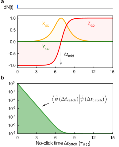
Фигура 3.1: Conditional no-click evolution of the jump from $\left|\mathrm{G}\right\rangle$ to $\left|\mathrm{D}\right\rangle$: ideal photodetection theory. a, A typical quantum trajectory for a jump from $\left|\mathrm{G}\right\rangle$ to $\left|\mathrm{D}\right\rangle$ represented as the GD Bloch vector ($X_{\mathrm{GD}}$, $Y_{\mathrm{GD}}$, $Z_{\mathrm{GD}}$), conditioned on no clicks, $\mathrm{d}N\left(t\right)=0$, for duration $\Delta t_{\mathrm{catch}}$. The Rabi drives are $\Omega_{\mathrm{DG}}=10^{-5}$ and $\Omega_{\mathrm{BG}}=0.1$ in units of the decay rate $\gamma_{\mathrm{B}}$. Time axis is scaled in units of the mean time between detector clicks, $\tau_{\mathrm{BG}}=(\Omega_{{\rm BG}}^{2}/\gamma_{\mathrm{B}})^{-1}$. Time scale of the jump flight is the mid-flight time $\Delta t_{\mathrm{mid}}$, defined by $Z_{\mathrm{GD}}=0$. b, Log plot of the norm of the un-normalized no-click state, $\left\langle\tilde{\psi}\left(\Delta t_{\mathrm{catch}}\right)\middle|\tilde{\psi}\left(\Delta t_{\mathrm{catch}}\right)\right\rangle$, as a function of $\Delta t_{\mathrm{catch}}$, in units of $\tau_{\mathrm{BG}}$. Parameters of the plot correspond to those of panel a.

Remarks on the state evolution.

The evolution of the GD manifold Bloch vector ($X_{\mathrm{GD}}\left(\Delta t_{\mathrm{catch}}\right),$ $Y_{\mathrm{GD}}\left(\Delta t_{\mathrm{catch}}\right),$ $Z_{\mathrm{GD}}\left(\Delta t_{\mathrm{catch}}\right)$) conditioned on no clicks, $\mathrm{d}N\left(\Delta t_{\mathrm{catch}}\right)=0$, for duration $\Delta t_{\mathrm{catch}}$, is plotted in Fig. 3.1a. The partial tomogram visually shows that the predicted evolution of the quantum jump from $\left|\mathrm{G}\right\rangle$ to $\left|\mathrm{D}\right\rangle$ is continuous and coherent, $X_{\mathrm{GD}}^{2}+Y_{\mathrm{GD}}^{2}+Z_{\mathrm{GD}}^{2}=1$ for all no-click times, $\Delta t_{\mathrm{catch}}$. The measurement record, $\mathrm{d}N$, and the predicted trajectory is identical for any two jumps from $\left|\mathrm{G}\right\rangle$ to $\left|\mathrm{D}\right\rangle$. The time axis has been scaled in units of the mean time, $\tau_{\mathrm{BG}}=(\Omega_{{\rm BG}}^{2}/\gamma_{\mathrm{B}})^{-1}$, between photon detector clicks. This time can also be understood as the inverse of the information-gain rate of the measurement about the G level. To expand on this, for definitiveness, consider the situation where the atom is initialized in $\left|\mathrm{G}\right\rangle$, but this information is not shared with the observer operating the photon detector. By measurement, how long does it take the observer to statistically deduce that the atom is in $\left|\mathrm{G}\right\rangle$ or not? The measurement drive $\Omega_{\mathrm{BG}}$ is actuated and the observer monitors the detector for clicks. If the atom is in $\left|\mathrm{G}\right\rangle,$ on average, the detector records a click after time $\tau_{\mathrm{BG}}$, and informs the observer that the atom is definitively in $\left|\mathrm{G}\right\rangle$. Alternatively, if the atom was initialized in $\left|\mathrm{D}\right\rangle,$ no clicks would be recorded. As the detector does not record a click for durations longer than $\tau_{{\rm BG}}$, the observer becomes increasingly confident that the atom could not be in $\left|\mathrm{G}\right\rangle$ since it becomes exponentially unlikely that a click has not yet been observed, see Fig. 3.1b, and the alternative conclusion, that the atom is in $\left|\mathrm{D}\right\rangle$, becomes increasingly likely. Although this information-gain consideration is carried out from the point of view of the observer, and with classical measurements would bear no consequence for the objective state of the system, with quantum measurements the gain of information about the system by virtue of a measurement is necessarily accompanied by a result-correlated state-disturbance (back-action). In Hilbert space, the disturbance can be viewed as a measurement-backaction effective force, as discussed in the following subsection, Sec. 3.1.2.

Probability of no-click record.

Fig. 3.1b shows a plot of the conditional no-click state norm, $\left\langle\psi\left(\Delta t_{\mathrm{catch}}\right)\middle|\psi\left(\Delta t_{\mathrm{catch}}\right)\right\rangle$, as a function of the no-click duration, $\Delta t_{\mathrm{catch}}$. The norm initially decays exponentially with a time-constant $\tau_{{\rm BG}}$, during which time, the atom remains essentially in $\left|\mathrm{G}\right\rangle$, as indicated by the $Z_{{\rm GD}}$ Bloch component in panel a, which is roughly equal to $-1$. However, as the no-click duration approaches mid-flight time of the jump, $\Delta t_{\mathrm{catch}}\approx\Delta t_{{\rm mid}}$, the decay of the norm slows down dramatically, since the atom transitions from $\left|\mathrm{G}\right\rangle$ to $\left|\mathrm{D}\right\rangle$, in which state one can stop expecting the rapid occurrence of clicks. The quantum jump from $\left|\mathrm{G}\right\rangle$ to $\left|\mathrm{D}\right\rangle$ can be observed in the tomogram shown in panel (a). For no-click duration $\Delta t_{\mathrm{catch}}\gg\Delta t_{{\rm mid}}$, the decay of the norm initially appears flat, however, on longer time-scales (not shown) it is seen that it also follows an exponential decay law with a much longer time constant, $\tau_{{\rm DG}}\gg\tau_{{\rm BG}}$, corresponding to the waiting-time for the jump back down, from $\left|\mathrm{D}\right\rangle$ to $\left|\mathrm{G}\right\rangle$.

Application of the photon counting model to the experiment.

The photon-counting theory presented in this section provides the background to the experiment along with a link to the original ion experiments. It captures a core set of the ideas, even though the monitoring of $|{\rm B\rangle}$ implemented in the experiment is diffusive — the opposite limit of the point-process description presented here, see Sec. 3.2. Nevertheless, the photon-counting theory even provides a quantitative first approximation of the experimental results. For definitiveness, consider the flight of the quantum jump shown in Fig. 1.3b. The measured mid-flight time, $\Delta t_{\mathrm{mid}}=3.95\leavevmode\nobreak\ \mathrm{\mu s}$, is predicted, in a first approximation, by Eq. (3.17). Using the (independently measured) values of the experimental parameters, summarized in Table 5.1 (setting $\Omega_{\mathrm{BG}}$ equal to $\Omega_{\mathrm{B0}}=2\pi\times 1.2$ MHz, the BG drive when the atom is not in $\left|\rm B\right\rangle$) and extracting the effective measurement rate of $|{\rm B\rangle}$, $\gamma_{\mathrm{B}}=2\pi\times 9.0$ MHz (which follows from Eq. (3.8) where $\Gamma_{\mathrm{BG}}=2\pi\times 1.01$ MHz, the average click rate on the BG transition), Eq. (3.17) predicts $\Delta t_{{\rm mid}}\approx 4.3\leavevmode\nobreak\ \mathrm{\mu s}$ — in fair agreement with the observed value $\Delta t_{{\rm mid}}=3.95\leavevmode\nobreak\ \mathrm{\mu s}$. The photodetection theory presented in in Sec. 3.1.3 further improves the agreement. These calculations serve to generally illustrate the theory and ideas of the experiment; the quantitative comparison between theory and experiment is only presented in Sec. 5.5.

3.1.2 Measurement-backaction effective force in the absence of the Dark Rabi drive

While in Sec. 3.1.1 we considered the coherent dynamics of the three-level atom in the presence of both unitary evolution, due to the Rabi drive $\Omega_{\mathrm{DG}}$, and the competing non-unitary state collapse, due to the measurement, in this subsection, we examine the simpler case where only measurement dynamics are at play, i.e., $\Omega_{\mathrm{DG}}=0$. In this simpler situation, some important features of the measurement, consisting of the Rabi drive $\Omega_{\mathrm{BG}}$ and the monitoring of the B level at the rate $\gamma_{{\rm B}}$, are more easily discussed. In particular, we pay attention to the notion of a measurement-backaction effective force, the special force that unavoidably disturbs of the quantum state due to the measurement.

For definitiveness, consider the situation where the three-level atom is prepared in an initial superposition involving the G and D levels, $\left|\psi\left(0\right)\right\rangle=\mathcal{N}\left(\left|\mathrm{G}\right\rangle+\epsilon\left|\mathrm{D}\right\rangle\right)$, where $\epsilon\ll 1$ and $\mathcal{N}$ is the ket normalization factor; for simplicity, assume $\left|\mathrm{D}\right\rangle$ is completely decoupled form the environment, $\gamma_{{\rm D}}=0$. To measure the atom, only the Rabi drive $\Omega_{\mathrm{BG}}$ is turned on. One of two qualitatively distinct measurement records is observed: either clicks are recorded indefinitely or no clicks are ever recorded, which can qualitatively be understood in view of the following considerations. When the BG drive is first turned on, some of the initial population from the G level is transferred to the B level due to the steering force of $\Omega_{\mathrm{BG}}$. However, even as a tiny amount of population is deposited in $\left|\mathrm{B}\right\rangle$, the strong coupling with the environment and the photodetector dampens the transfer and quickly yields the detection of a click, with probability $\wp_{1}\left(\mathrm{d}t\right)=\left\langle\hat{c}_{{\rm B}}^{\dagger}\hat{c}_{{\rm B}}\right\rangle\left(t\right)\mathrm{d}t$, where $\hat{c}_{\mathrm{B}}=\sqrt{\gamma_{{\rm B}}}\left|\mathrm{G}\right\rangle\left\langle\mathrm{B}\right|$ is the jump operator. The click resets the atom to the ground state, $\left|\mathrm{G}\right\rangle$. Once the atom is completely in $\left|\mathrm{G}\right\rangle$, the amplitude of $\left|\mathrm{D}\right\rangle$ is zero, and since $\Omega_{\mathrm{DG}}=0$, the atom can never transition to $\left|\mathrm{D}\right\rangle$ subsequently. The remainder of the history proceeds as described above, the atom remains predominantly in $\left|\mathrm{G}\right\rangle$ and continues to fluoresce though the partial excitation and subsequent relaxation of $\left|\mathrm{B}\right\rangle$, by means of $\Omega_{\mathrm{BG}}$ and the detection, $\gamma_{{\rm B}}$, respectively. In this way, the Dehmelt electron scheme implements a measurement with result $\left|\mathrm{G}\right\rangle$, occurring with an approximate probability $1-\epsilon^{2}$. The alternative set of trajectories, where no clicks are observed is quantitatively analyzed in the following, and occur with approximate probability $\epsilon^{2}$.

No-click trajectory.

The normalized state of the three-level atom conditioned on no-clicks,

$$\left|\psi_{I=0}\left(t\right)\right\rangle=C_{\mathrm{G}}\left(t\right)\left|\mathrm{G}\right\rangle+C_{\mathrm{B}}\left(t\right)\left|\mathrm{B}\right\rangle+C_{\mathrm{D}}\left(t\right)\left|\mathrm{D}\right\rangle\,,$$ (3.21)

evolves according to the non-linear Schrödinger equation, see Eq. (3.10),

$$\frac{\mathrm{d}}{\mathrm{d}t}\left|\psi_{I=0}\left(t\right)\right\rangle=\left(-i\hat{H}-\frac{1}{2}\hat{c}_{{\rm B}}^{\dagger}\hat{c}_{{\rm B}}+\frac{1}{2}\left\langle\hat{c}_{{\rm B}}^{\dagger}\hat{c}_{{\rm B}}\right\rangle\left(t\right)\right)\left|\psi_{I=0}\left(t\right)\right\rangle\>,$$ (3.22)

which in terms of the normalized state coefficients ($C_{\mathrm{G}},C_{\mathrm{B}}$, and $C_{\mathrm{D}}$) yields the set of coupled non-linear equations,

$$\frac{\mathrm{d}}{\mathrm{d}t}C_{\mathrm{B}}\left(t\right)= \frac{1}{2}\gamma_{{\rm B}}C_{\mathrm{B}}\left(t\right)^{3}+\frac{1}{2}\Omega_{{\rm BG}}C_{\mathrm{G}}\left(t\right)-\frac{1}{2}\gamma_{{\rm B}}C_{\mathrm{B}}\left(t\right),$$ (3.23)

$$\frac{\mathrm{d}}{\mathrm{d}t}C_{\mathrm{G}}\left(t\right)= \frac{1}{2}\gamma_{{\rm B}}C_{\mathrm{B}}\left(t\right)^{2}C_{\mathrm{G}}\left(t\right)-\frac{1}{2}\Omega_{{\rm BG}}C_{\mathrm{B}}\left(t\right),$$ (3.24)

$$\frac{\mathrm{d}}{\mathrm{d}t}C_{\mathrm{D}}\left(t\right)= \frac{1}{2}\gamma_{{\rm B}}C_{\mathrm{B}}\left(t\right)^{2}C_{\mathrm{D}}\left(t\right),$$ (3.25)

The measurement terms in Eqs. (3.23)-(3.25) associated with information gain are the non-linear ones. As discussed in Sec. 2.3, they originate from the normalization term in the conditional state update and give rise to non-unitary state dynamics, resulting in a drastic departure from the usual Schrödinger equation. To analyze their effect and gain some physical intuition, we introduce a graphical representation of the Hilbert space of the three-level atom.

$\mathbb{R}$-qutrit sphere representation.

It follows from the real coefficients of Eqs. (3.23)-(3.25) and the initial conditions that $C_{\mathrm{G}},C_{\mathrm{B}},$ and $C_{\mathrm{D}}$ are constrained to be real. Hence a pure state of the atom admits a geometrical representation as a point on the unit sphere defined by the state norm condition $C_{\mathrm{B}}^{2}+C_{\mathrm{G}}^{2}+C_{\mathrm{D}}^{2}=1$, see Fig. 3.2. We nickname this representation the ’$\mathbb{R}$-qutrit sphere’. Unlike the Bloch sphere representation where orthogonal state vectors are represented by antiparallel vectors, in the $\mathbb{R}$-qutrit sphere representation, orthogonal state vectors are actually represented by orthogonal vectors, extending from the origin to the surface of the sphere. Notably, the sphere contains states of the two-level sub-manifolds that are not represented on the Bloch sphere, those with a ‘‘global phase.’’ The addition of the third level allows, in general, the observation of the global phase because it can be measured relative to the phase of the third level. Consequently, a Rabi rotation between two levels is no longer $2\pi$ periodic but $4\pi$ periodic. Unitary evolution is represented by rotations on the sphere; for instance, the evolution due to the Bright Rabi drive, $\Omega_{\mathrm{BG}}$, is a rotation about the D axis, and the corresponding infinitesimal-state-change vector field, $\mathrm{d}\left|\psi\right\rangle\left(\Omega_{\mathrm{BG}}\right)=\frac{1}{2}\left(C_{\mathrm{G}}\left|\mathrm{B}\right\rangle-C_{\mathrm{B}}\left|\mathrm{G}\right\rangle\right)\Omega_{\mathrm{BG}}\mathrm{d}t$, is plotted on the surface of the sphere in Fig. 3.2. Note that the length of the vectors is largest at the GB equator and approaches zero toward the D poles. The vector field representation is useful in the analysis of the non-linear measurement-backaction effective force due to the renormalization terms and we hope can provide a more intuitive understanding of the interplay between the coherent Rabi and the stochastic measurement dynamics. Before elaborating on the geometrical representation of the measurement dynamics, it is useful to first algebraically solve Eqs. (3.23)-(3.25).

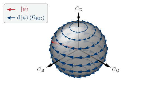
Фигура 3.2: Geometrical representation of a qutrit state with real coefficients: $\mathbb{\mathbb{R}}$-qutrit sphere. Geometric representation of the Hilbert space of pure states of a qutrit, $\left|\psi\right\rangle=C_{\mathrm{B}}\left|\mathrm{B}\right\rangle+C_{\mathrm{G}}\left|\mathrm{G}\right\rangle+C_{\mathrm{D}}\left|\mathrm{D}\right\rangle$, with real-valued coefficients, notably isomorphic to the special orthogonal group $SO\left(3\right)$. Overlaid vector field represents the infinitesimal state change, $\mathrm{d}\left|\psi\right\rangle$, due to the Rabi drive $\Omega_{{\rm BG}}.$

Measurement-backaction force steers atom towards $\left|\mathrm{D}\right\rangle$.

Although there is no Rabi drive or measurement directly applied to the Dark level, conditioned on not detecting a click, according to Eq. (3.25), a force is nonetheless exerted by the B-level monitoring that steers the atom toward the Dark level. Specifically, the rate of change of the D level amplitude, $\frac{\mathrm{d}}{\mathrm{d}t}C_{\mathrm{D}}$, is given by an anti-damping term with a state-dependent rate proportional to the B level population, $C_{\mathrm{B}}\left(t\right)^{2}$, and measurement rate, $\gamma_{{\rm B}}$. Solving Eq. (3.25), one finds

$$C_{\mathrm{D}}\left(t\right)=C_{\mathrm{D}}\left(0\right)\exp\left(\int_{0}^{t}\mathrm{d}t^{\prime}\frac{1}{2}\gamma_{{\rm B}}C_{\mathrm{B}}\left(t\right)^{2}\right)\,.$$ (3.26)

In this sense, the renormalization of the conditional state amounts to a (non-unitary) measurement-backaction force on $\left|\mathrm{D}\right\rangle$, which is linked to the population of $\left|\mathrm{B}\right\rangle.$ To explicitly solve Eq. (3.26), we need to solve the remaining equations, Eqs. (3.23) and (3.24).

Adiabatic elimination of the Bright state dynamics.

Because Eq. (3.23) is non-linear, we consider the B level dynamics and their adiabatic elimination with greater care. Eq. (3.23), contains both a damping, $-\frac{1}{2}\gamma_{{\rm B}}C_{\mathrm{B}}$, and an anti-damping, $\frac{1}{2}\gamma_{{\rm B}}C_{\mathrm{B}}{}^{3}$, term. These cancel out perfectly only if the atom is either entirely in $\left|\mathrm{B}\right\rangle$, $C_{\mathrm{B}}=\pm 1$, or not at all in $\left|\mathrm{B}\right\rangle$, $C_{\mathrm{B}}=0$; otherwise, $\left|C_{\mathrm{B}}\right|<1$, the damping dominates, steering $C_{\mathrm{B}}$ in the direction of zero. In the extreme case, where $\Omega_{{\rm BG}}=0$, one can explicitly solve the B level dynamics, $C_{\mathrm{B}}\left(t\right)^{2}=\left[1+\left(C_{\mathrm{B}}\left(0\right)^{-2}-1\right)\exp\left(\gamma_{{\rm B}}t\right)\right]^{-1},$ which for small initial populations, $C_{\mathrm{B}}\left(0\right)^{2}\ll 1$ rapidly decays to a stable zero equilibrium at a rate $\frac{1}{2}\gamma_{{\rm B}}$, $C_{\mathrm{B}}\left(t\right)\approx C_{\mathrm{B}}\left(0\right)\exp\left(-\frac{1}{2}\gamma_{{\rm B}}t\right)$. Since $\gamma_{{\rm B}}$ is the fastest timescale in the problem and the B dynamics are convergent, we can adiabatically eliminate $C_{\mathrm{B}}$ by setting $\frac{\mathrm{d}}{\mathrm{d}t}C_{\mathrm{B}}\left(t\right)=0$; solving the cubic equation, one finds three solution branches,

$$\bar{C}_{\mathrm{B}}\left(t\right)=\begin{cases}-1-\frac{\Omega_{\mathrm{BG}}}{2\gamma_{{\rm B}}}C_{\mathrm{G}}\left(t\right)+\mathcal{O}\left(\left(\Omega_{\mathrm{BG}}/\gamma_{{\rm B}}\right)^{2}\right)\\ 1-\frac{\Omega_{\mathrm{BG}}}{2\gamma_{{\rm B}}}C_{\mathrm{G}}\left(t\right)+\mathcal{O}\left(\left(\Omega_{\mathrm{BG}}/\gamma_{{\rm B}}\right)^{2}\right)\\ \frac{\Omega_{\mathrm{BG}}}{\gamma_{{\rm B}}}C_{\mathrm{G}}\left(t\right)+\mathcal{O}\left(\left(\Omega_{\mathrm{BG}}/\gamma_{{\rm B}}\right)^{3}\right)\,.\end{cases}$$ (3.27)

Operating the three-level atom in the limit where the $\left|\mathrm{B}\right\rangle$ level is never appreciably populated, we employ the third solution branch, $\bar{C}_{\mathrm{B}}\left(t\right)=\frac{\Omega_{\mathrm{BG}}}{\gamma_{{\rm B}}}C_{\mathrm{G}}\left(t\right)$, in Eq. (3.24) to find the effective equation of motion for the G level dynamics,

$$\frac{\mathrm{d}}{\mathrm{d}t}C_{\mathrm{G}}\left(t\right)=-\tau_{\mathrm{BG}}^{-1}\left[1-C_{\mathrm{G}}\left(t\right)^{2}\right]C_{\mathrm{G}}\left(t\right),$$ (3.28)

which are now completely decoupled from the other levels. In Eq. (3.28), we identify a damping and an anti-damping term with a constant and G-population dependent, $C_{\mathrm{G}}^{2}$, rate, respectively. The scale of both terms is given by the parameter $\tau_{\mathrm{BG}}^{-1}=\Omega_{{\rm BG}}^{2}/2\gamma_{\mathrm{B}}$, which is the expected rate of clicks when the atom is in $\left|\mathrm{G}\right\rangle$. By eliminating the B level, we have obtained an explicit relation for the effective monitoring of the G level, which occurs at a rate $\tau_{{\rm BG}}^{-1}$, which can also be interpreted as the quantum Zeno rate (Misra and Sudarshan, 1977, Gambetta et al., 2008, Matsuzaki et al., 2010, Vijay et al., 2011, Slichter et al., 2016, Harrington et al., 2017, Hacohen-Gourgy et al., 2018). The numerator $\Omega_{\mathrm{BG}}^{2}$ is proportional to the population transfer rate from $\left|\mathrm{G}\right\rangle$ to $\left|\mathrm{B}\right\rangle$ while the denominator $\gamma_{{\rm B}}$ gives the rate of projection from $\left|\mathrm{B}\right\rangle$ to $\left|\mathrm{G}\right\rangle$. Solving Eq. (3.28) and substituting its solution in Eq. (3.26), one finds

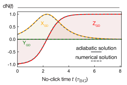
Фигура 3.3: Adiabatic solution for the no-click GD manifold trajectory of a superposition state measured with $\Omega_{\mathrm{DG}}=0$. Adiabatic-approximation (solid lines) and numerical (dashed lines) solution for the partial tomogram of the GD manifold of the no-click quantum trajectory of an initial superposition state $\left|\psi\left(0\right)\right\rangle=\mathcal{N}\left(\left|\mathrm{G}\right\rangle+\epsilon\left|\mathrm{D}\right\rangle\right)$, where $\epsilon=0.1$ and $\mathcal{N}=\left(1+\epsilon^{2}\right)^{-1/2}$. The Bright Rabi drive is $\Omega_{\mathrm{BG}}=0.1$, in units of the decay rate $\gamma_{{\rm B}}$. Time axis scaled in units of $\tau_{\mathrm{BG}}=\left(\Omega_{\mathrm{BG}}^{2}/\gamma_{{\rm BG}}\right)^{-1}.$

$$C_{\mathrm{G}}\left(t\right)^{2}= \frac{p_{{\rm G}}}{p_{{\rm G}}+\left(1-p_{{\rm G}}\right)e^{2t/\tau_{{\rm BG}}}}\,,$$ (3.29)

$$C_{\mathrm{D}}\left(t\right)^{2}= \frac{p_{{\rm D}}e^{t/\tau_{{\rm BG}}}}{p_{{\rm D}}+\left(1-p_{{\rm D}}\right)e^{2t/\tau_{{\rm BG}}}}\,,$$ (3.30)

where $p_{{\rm G}}\equiv C_{\mathrm{G}}\left(0\right)^{2}$ and $p_{{\rm D}}\equiv C_{\mathrm{D}}\left(0\right)^{2}$ are the initial conditions. Note, for $p_{{\rm D}}=0$, the above solution for $C_{\mathrm{D}}$ is always zero. The evolution of the GD Bloch vector conditioned on no clicks for the initial state $\left|\psi\left(0\right)\right\rangle=\mathcal{N}\left(\left|\mathrm{G}\right\rangle+\epsilon\left|\mathrm{D}\right\rangle\right)$ is obtained by substituting Eq. (3.29) and (3.30) in Eqs. (3.11)-(3.13),

$${\rm Z}_{{\rm GD}}(t) ={\rm tanh}\left[t/\tau_{{\rm BG}}+\mathrm{arctanh}\left[{\rm Z}_{{\rm GD}}(0)\right]\right],$$ (3.31)

$${\rm X}_{{\rm GD}}(t) ={\rm sech}\left[t/\tau_{{\rm BG}}+\mathrm{arctanh}\left[{\rm Z}_{{\rm GD}}(0)\right]\right],$$ (3.32)

$${\rm Y}_{{\rm GD}}(t) =0.$$ (3.33)

We note that a few results of this subsection, especially Eqs. (3.31)-(3.33), bear resemblance to results from Sec. 3.1.1, yet we stress that the two situations are fundamentally distinct, and the resemblance must be considered with care. For instance, we note that the mid-flight time $\Delta t_{\mathrm{mid}}$ cannot be recovered from the simpler situation considered here, where no quantum jumps occur and there is no competition between unitary dynamics due to $\Omega_{{\rm DG}}$ and the measurement.

In Fig. 3.3a, we plot the adiabatic-approximation solution to the non-linear Schrödinger evolution, Eq. (3.22), for the GD manifold Bloch vector conditioned on no clicks, Eqs. (3.31)-(3.33), obtained in the limit $\Omega_{\mathrm{BG}}\ll\gamma_{B}$. Overlaid (dashed lines) is the corresponding numerically calculated solution to Eq. (3.22). Even for modest separation of timescales, $\Omega_{\mathrm{BG}}/\gamma_{{\rm B}}=0.1$ in the plot, the two solutions appear nearly indistinguishable. The initial atom state, $\epsilon=0.1$, is gradually projected to $\left|\mathrm{D}\right\rangle$ on a timescale given by $\tau_{{\rm BG}}$ and evolves in a characteristically non-unitary manner. Notably, the state remains pure at all times, and in the limit $t\gg\tau_{{\rm BG}}$ remains essentially in $\left|\mathrm{D}\right\rangle$, indefinitely. Importantly, for times $t$ on the other of $\tau_{{\rm BG}}$, the projection can (but need not) be interrupted by the detection of a click, which would project the state to $\left|\mathrm{G}\right\rangle$, and occurs with total probability $\approx 1-\epsilon^{2}$.

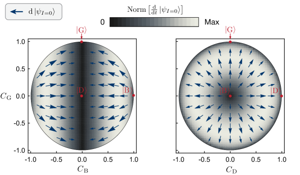
Фигура 3.4: Geometrical representation of the no-click measurement-backaction force for $\Omega_{\mathrm{BG}}=0$. Shown are two projections of $\mathbb{\mathbb{\mathbb{R}}}$-qutrit sphere overlaid with the measurement-force vector field, $\frac{\mathrm{d}}{\mathrm{d}t}\left|\psi_{I=0}\right\rangle$, due to the monitoring of the B level with $\Omega_{\mathrm{BG}}=0$. Color of density plot indicates the relative magnitude of the change, $\mathrm{Norm}\left[\frac{\mathrm{d}}{\mathrm{d}t}\left|\psi_{I=0}\right\rangle\right]$.

Hilbert space representation of the measurement dynamics.

It is useful to consider a geometric representation of the measurement dynamics and in particular of the non-linear measurement-backaction force. For simplicity, first consider the measurement force due only to the monitoring of the B level, in the absence of the Bright Rabi drive, $\Omega_{\mathrm{BG}}=0$. This force can be represented as a vector field on the surface of the $\mathbb{R}$-qutrit sphere, see Fig. 3.4. The vector field is calculated from Eqs. (3.31)-(3.33) for the change in the state conditioned on detecting no clicks,

$$\frac{\mathrm{d}}{\mathrm{d}t}\left|\psi_{I=0}\right\rangle=\frac{1}{2}\gamma_{{\rm B}}C_{\mathrm{B}}{}^{2}\begin{pmatrix}C_{\mathrm{B}}-1\\ C_{\mathrm{G}}\\ C_{\mathrm{D}}\end{pmatrix}\,.$$ (3.34)

The colormap in Fig. 3.4 depicts the relative magnitude of the change, $\mathrm{Norm}\left[\frac{\mathrm{d}}{\mathrm{d}t}\left|\psi_{I=0}\right\rangle\right],$ which we note is only zero in two special cases: i) when the atom is $\pm\left|\mathrm{B}\right\rangle$, corresponding to the points $\left(\pm 1,0,0\right),$ and ii) when the atom is in a state involving exclusively $\left|\mathrm{G}\right\rangle$ and $\left|\mathrm{D}\right\rangle$ but not $\left|\mathrm{B}\right\rangle$. The latter is special in that it corresponds to an entire manifold of states, the GD equatorial circle, which can be visually recognized in Fig. 3.4 as the dark vertical stripe at the center of the left panel and the dark circular perimeter of the disk in the right panel. All other states, not covered under the latter two cases, are superpositions involving $\left|\mathrm{B}\right\rangle$. From the vector field plot, it is evident that these states are guided by the force away from the $\left|\mathrm{B}\right\rangle$ poles and toward the GD equator. It is precisely this feature of the measurement force that results in the gradual projection of the state conditioned on no clicks — it is the unavoidable disturbance of the atom due to the information-gain of the no-click measurement outcomes, which lead the observer to gradually learn that the atom is not in $\left|\mathrm{D}\right\rangle$, thus resulting in the increased likelihood that it is in $\left|\mathrm{G}\right\rangle$ or $\left|\mathrm{D}\right\rangle$. This dynamics embody the message of the Chapter 2 epigraph, ‘‘In quantum physics you don’t see what you get, you get what you see.’’

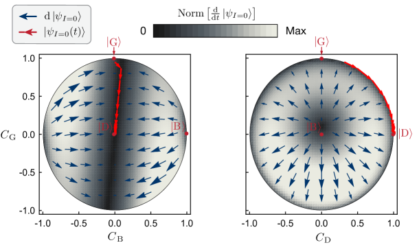
Фигура 3.5: Geometrical representation of the measurement-backaction force and a no-click trajectory with $\Omega_{\mathrm{BG}}=0.1\gamma_{{\rm B}}$. Two projections of the $\mathbb{\mathbb{\mathbb{R}}}$-qutrit sphere overlaid with the measurement-force vector field $\frac{\mathrm{d}}{\mathrm{d}t}\left|\psi_{I=0}\right\rangle$ (blue arrows) and the path of the quantum trajectory from Fig. (3.3) (red arrows), depicting the gradual projection of a superposition state to $\left|\mathrm{D}\right\rangle$ conditioned on no clicks. Density plot indicates relative field magnitude, $\mathrm{Norm}\left[\frac{\mathrm{d}}{\mathrm{d}t}\left|\psi_{I=0}\right\rangle\right]$.

In Fig. 3.5, we plot the measurement vector field in the presence of the Bright Rabi drive $\Omega_{\mathrm{BG}}$,

$$\frac{\mathrm{d}}{\mathrm{d}t}\left|\psi_{I=0}\right\rangle=\frac{1}{2}\gamma_{{\rm B}}C_{\mathrm{B}}{}^{2}\begin{pmatrix}C_{\mathrm{B}}-1\\ C_{\mathrm{G}}\\ C_{\mathrm{D}}\end{pmatrix}+\frac{1}{2}\Omega_{\mathrm{BG}}\begin{pmatrix}C_{\mathrm{G}}\\ -C_{\mathrm{B}}\\ 0\end{pmatrix}\,,$$ (3.35)

with $\Omega_{\mathrm{BG}}=0.1\gamma_{{\rm B}}$. The Bright Rabi drive, visually represented on the $\mathbb{R}$-qutrit sphere in Fig. 3.2, perturbs the measurement field, shown in Fig. 3.4, by linking the B and G levels and lifting the degeneracy of the measurement, represented in GD equator. Visually, this is evident in the tilt of the vertical dark stripe in the center of the left-panel colormap. In the right panel, it is also evident that $\left|\mathrm{B}\right\rangle$ is no longer an equilibrium point; the equilibrium has been shifted in the direction of $\left|\mathrm{G}\right\rangle$ by an amount proportional $\Omega_{\mathrm{BG}}/\gamma_{{\rm B}},$ see Eq. (3.27), and made metastable. The red arrows depict the path of the quantum trajectory in Hilbert of the gradual projection of an initial superposition state of $\left|\mathrm{G}\right\rangle$ and $\left|\mathrm{D}\right\rangle$, for the same parameters as employed in Fig. (3.3), where $\epsilon=0.1$. Initially, the state is quickly steered in the direction of $\left|\mathrm{B}\right\rangle$ by the force of $\Omega_{\mathrm{BG}}$. However, as the state moves in the direction of $\left|\mathrm{B}\right\rangle$, the motion is quickly opposed by the no-click measurement-backaction force, which grows larger in amplitude in this direction. The two forces do not precisely cancel each other out, because of the slight mismatch in angles. The net force, albeit small, steers the atom towards the GD equator and with a slight tilt toward $\left|\mathrm{D}\right\rangle$. The opposition of the $\Omega_{\mathrm{BG}}$ drive and the measurement back-action ‘‘trap’’ the state in the ridge where the two forces nearly cancel each other out, the nearly vertical dark stripe in the left panel, and the small angular mismatch slowly carries the state in the direction of $\left|\mathrm{D}\right\rangle$, an equilibirum point, where all forces are zero.

3.1.3 Incoherent Bright drive and Dark drive off

In this section, we consider the case of quantum jumps in the three-level atom subject to photodetection and an incoherent Bright drive, rather than a Rabi one, see Sec. 3.1.1. The situation analyzed in this section is somewhat more analogous to the cQED experiment where the Bright Rabi drive consists of a bi-chromatic tone that unconditionally addresses the BG transition, independent of the population of the readout cavity, necessitated by the dispersive pull of the readout cavity on the BG frequency. The bi-chromatic drive effectively acts as an incoherent drive. The incoherent Bright drive photodetection theory presented here sheds some further light on the dynamics of the quantum jump from $\left|\mathrm{G}\right\rangle$ to $\left|\mathrm{D}\right\rangle$. Features such as the non-zero coherence, $X_{{\rm GD}}$, and in the limit $\Delta t_{\mathrm{catch}}\gg\Delta t_{{\rm mid}}$ are discussed.

Replacing the coherent Rabi drive $\Omega_{{\rm BG}}$ by an incoherent drive $\Gamma_{{\rm BG}}$ in the master equation of the three-level atom in the interaction picture, Eq. (3.1) becomes

$$\frac{\mathrm{d}\rho}{\mathrm{d}t}=(i\hbar)^{-1}[\hat{H}_{{\rm drive}},\rho]+\Gamma_{{\rm BG}}{\cal D}\left[\left|\rm B\right\rangle\left\langle\rm G\right|\right]\rho+(\gamma_{{\rm B}}+\Gamma_{{\rm BG}}){\cal D}\left[\left|\rm G\right\rangle\left\langle\rm B\right|\right]\rho+\gamma_{{\rm D}}{\cal D}\left[\left|\rm G\right\rangle\left\langle\rm D\right|\right]\rho,$$ (3.36)

and Eq. (3.5) becomes

$$\hat{H}_{{\rm drive}}=i\hbar\frac{\Omega_{{\rm DG}}}{2}\big{(}\left|\rm D\right\rangle\left\langle\rm G\right|-\left|\rm G\right\rangle\left\langle\rm D\right|\big{)}.$$ (3.37)

The strong-monitoring assumption, $\tau_{{\rm BG}}^{-1}\ll\gamma_{{\rm B}}$, is also carried over from Sec. 3.1.1 by assuming $\Gamma_{{\rm BG}}\ll\gamma_{{\rm B}}$, i.e., the time between clicks in fluorescence is essentially the same as the time separating photon absorptions from the incoherent drive, as absorption is rapidly followed by fluorescence ($\gamma_{{\rm B}}+\Gamma_{{\rm BG}}\gg\Gamma_{{\rm BG}}$). This brings a useful simplification, since, following each reset to $\left|\mathrm{G}\right\rangle$, the unnormalized state evolves in the GD-subspace,

$$i\hbar\frac{\mathrm{d}\left|\tilde{\psi}\right\rangle}{\mathrm{d}\Delta t_{{\rm catch}}}=\left(\hat{H}_{{\rm drive}}-i\hbar\frac{\Gamma_{{\rm BG}}}{2}\left|\rm G\right\rangle\left\langle\rm G\right|-i\hbar\frac{\gamma_{{\rm D}}}{2}\left|\rm D\right\rangle\left\langle\rm D\right|\right)\left|\tilde{\psi}\right\rangle,$$ (3.38)

thus replacing Eqs. (3.7) and (3.15) by the simpler $2\times 2$ system

$$\frac{\mathrm{d}}{\mathrm{d}\Delta t_{{\rm catch}}}\begin{pmatrix}c_{\mathrm{G}}\\ c_{\mathrm{D}}\end{pmatrix}=\frac{1}{2}\left(\begin{matrix}-\Gamma_{{\rm BG}}&-\Omega_{{\rm DG}}\\ \Omega_{{\rm DG}}&-\gamma_{{\rm D}}\end{matrix}\right)\begin{pmatrix}c_{\mathrm{G}}\\ c_{\mathrm{D}}\end{pmatrix},$$ (3.39)

and, in the limit $\gamma_{{\rm D}}\ll\Gamma_{{\rm BG}}$, the equation of motion for $W_{{\rm DG}}$, defined in Eq. (3.14), is

$$\frac{\mathrm{d}W_{{\rm DG}}}{\mathrm{d}\Delta t_{{\rm catch}}}=\frac{\Gamma_{{\rm BG}}}{2}W_{{\rm DG}}+\frac{\Omega_{{\rm DG}}}{2}(1+W_{{\rm DG}}^{2}),$$ (3.40)

with solution, for $W_{{\rm DG}}(0)=0$,

$$W_{{\rm DG}}(\Delta t_{{\rm catch}})=\frac{\exp\left[(V-V^{-1})\Omega_{{\rm DG}}\Delta t_{{\rm catch}}/2\right]-1}{V-V^{-1}\exp\left[(V-V^{-1})\Omega_{{\rm DG}}\Delta t_{{\rm catch}}/2\right]},$$ (3.41)

where

$$V=\frac{1}{2}\frac{\Gamma_{{\rm BG}}}{\Omega_{{\rm DG}}}+\sqrt{\frac{1}{4}\left(\frac{\Gamma_{{\rm BG}}}{\Omega_{{\rm DG}}}\right)^{2}-1}.$$ (3.42)

In Ref. Ruskov et al. (2007), a general form of the Bloch vector equations for arbitrary amplitude of the Rabi drive was found. Inversion of the condition $W_{{\rm DG}}(\Delta t_{{\rm mid}})=1$ gives the characteristic time scale

$$\Delta t_{{\rm mid}}=2\left[(V-V^{-1})\Omega_{{\rm DG}}\right]^{-1}\ln\left(\frac{V+1}{V^{-1}+1}\right).$$ (3.43)

Although Eqs. (3.41) and (3.43) replace Eqs. (3.16) and (3.17), under strong monitoring, $\Gamma_{{\rm BG}}\gg\Omega_{{\rm DG}}$, they revert to the latter with the substitution $\Omega_{{\rm BG}}^{2}/2\gamma_{{\rm B}}\to\Gamma_{{\rm BG}}/2$,; in this way, Eqs. (3.11)–(3.13) are recovered with the same substitution. More generally, $W_{{\rm DG}}(\Delta t_{{\rm catch}})$ goes to infinity at finite $\Delta t_{{\rm catch}}$, changes sign, and returns from infinity to settle on the steady value $W_{{\rm DG}}(\infty)=-V$. The singular behavior marks a trajectory passing through the north pole of Bloch sphere. It yields the long-time solution

$${\rm Z}_{{\rm GD}}(\infty)=\sqrt{1-4\left(\frac{\Omega_{{\rm DG}}}{\Gamma_{{\rm BG}}}\right)^{2}},\qquad{\rm X}_{{\rm GD}}(\infty)=-2\frac{\Omega_{{\rm DG}}}{\Gamma_{{\rm BG}}},\qquad{\rm Y}_{{\rm GD}}(\infty)=0,$$ (3.44)

in contrast to the perfect jump of Eqs. (3.18)–(3.20). The long-term coherence and lower-than-one value of Z were observed in the experiments, see Fig. 1.3b. They can be understood as the equilibrium point of the coherent Rabi drive $\Omega_{{\rm DG}}$ attempting to rotate the state from $\left|\mathrm{D}\right\rangle$ back to $\left|\mathrm{G}\right\rangle$ perfectly balanced against the measurement-backaction force of the no-click measurement steering the atom toward $\left|\mathrm{D}\right\rangle$, recall discussion of the measurement vector field, see Figs. 3.4 and 3.5.

Dark drive off.

Turing the Dark drive off shortly after a click demonstrates the connection between the flight of a quantum jump and a projective measurement. From the point of view of the trajectory equations, the only change is the setting of $\Omega_{{\rm DG}}$ to zero at time $\Delta t_{{\rm on}}$ on the right-hand side of Eqs. (3.15) and (3.40). Subsequently, $W_{{\rm DG}}(\Delta t_{{\rm catch}})$ continues its exponential growth at rate $\Omega_{{\rm BG}}^{2}/2\gamma_{B}$ [Eq. (3.15)] or $\Gamma_{{\rm BG}}/2$ [Eq. (3.40)]. Equations (3.11)–(3.13) for the GD Bloch components still hold, but now with

$$\Delta t_{{\rm mid}}=\left(\frac{\Omega_{{\rm BG}}^{2}}{2\gamma_{B}},\frac{\Gamma_{{\rm BG}}}{2}\right)^{-1}\ln\big{[}W_{{\rm DG}}^{-2}(\Delta t_{{\rm on}})\big{]}.$$ (3.45)

which can provide an estimate of $\Delta t^{\prime}_{\mathrm{mid}}$, specifying the time at which $Z_{\mathrm{GD}}=0$.

The evolution during $\Delta t_{\mathrm{off}}$, in the absence of $\Omega_{\mathrm{DG}}$, in effect realizes a projective measurement of whether the state of the atom is $\left|\mathrm{G}\right\rangle$ or $|{\rm D}\rangle$, similar to the one analyzed in Sec. 3.1.2, where the normalized state at $\Delta t_{{\rm on}}$ is

$$\frac{|\psi(\Delta t_{{\rm on}})\rangle}{\sqrt{\mathcal{N}(\Delta t_{{\rm on}})}}=\frac{c_{\mathrm{G}}(\Delta t_{{\rm on}})\left|\mathrm{G}\right\rangle+c_{\mathrm{D}}(\Delta t_{{\rm on}})\left|\mathrm{D}\right\rangle}{\sqrt{\mathcal{N}(\Delta t_{{\rm on}})}},$$ (3.46)

with $\mathcal{N}(\Delta t_{{\rm on}})=c_{\mathrm{G}}^{2}(\Delta t_{{\rm on}})+c_{\mathrm{D}}^{2}(\Delta t_{{\rm on}})$ the probability for the jump to reach $\Delta t_{{\rm catch}}=\Delta t_{{\rm on}}$ after a click reset to $\left|\mathrm{G}\right\rangle$ at $\Delta t_{{\rm catch}}=0$. The probability for the jump to continue to $\Delta t_{{\rm catch}}>\Delta t_{{\rm on}}$ (given $\Delta t_{{\rm on}}$ is reached) is then

$$\frac{\mathcal{N}(\Delta t_{{\rm catch}})}{\mathcal{N}(\Delta t_{{\rm on}})}=\frac{C_{{\rm D}}^{2}(\Delta t_{{\rm on}})}{\mathcal{N}(\Delta t_{{\rm on}})}+\frac{C_{{\rm G}}^{2}(\Delta t_{{\rm on}})}{\mathcal{N}(\Delta t_{{\rm on}})}\exp\left[-\left(\frac{\Omega_{{\rm BG}}^{2}}{\gamma_{{\rm B}}},\Gamma_{{\rm BG}}\right)\Delta t_{{\rm catch}}\right].$$ (3.47)

Completed and aborted evolutions of the jump transition.

In this simple model, the probability for the trajectory to complete — for the measurement to yield the result $|{\rm D}\rangle$ — is obtained in the limit $\Delta t_{\mathrm{catch}}\rightarrow\infty$, and, as expected, is equal to the probability to occupy the state $|{\rm D}\rangle$ at time $\Delta t_{{\rm on}}$; i.e., the completion probability is $P_{\mathrm{D}}(\Delta t_{{\rm on}})=C_{{\rm D}}^{2}(\Delta t_{{\rm on}})/{{\rm Norm}(\Delta t_{{\rm on}})}$. It is helpful to illustrate this idea with an example. Consider the catch experiment of Fig. 1.3b in the absence of the Dark Rabi drive, $\Omega_{\mathrm{DG}}$. From $Z_{\mathrm{GD}}$, we can estimate that out of all the trajectories that pass though the $\Delta t_{{\rm on}}$ mark approximately $P_{\mathrm{D}}(\Delta t_{{\rm on}})=(1+Z_{\mathrm{GD}}(\Delta t_{{\rm on}}))/2\approx 8\%$ fully complete without an interruption. On the other hand, for those that pass the $\Delta t^{\prime}_{\mathrm{mid}}$ mark, approximately 50% complete. It follows from Eq. (3.47), that the probability of the evolution to complete increases the further along the trajectory is. Although some of the jump evolutions abort at random, importantly, every single jump evolution that completes, and is thus recorded as a jump, follows not a random but an identical path in Hilbert space, i.e., a deterministic one. This path (of any jump) is determined by Eq. (3.41), or, in the simpler model, by the Eqs. (3.18)-(3.20) for the components of the GD Bloch vector.

3.2 Heterodyne monitoring of readout cavity coupled to three-level atom

3.2.1 Description of cQED experiment

In Chapter 1, we described the cQED experiment involving a superconducting atom with the necessary V-shape level structure (see Fig. 1.1a or Sec. 4.1) subject to heterodyne monitoring of $\left|\mathrm{B}\right\rangle$ by means a dispersively coupled readout cavity. The three-level atom is formed form two heavily hybridized transmon modes, which are coupled by means of a cross-Kerr interaction to the readout cavity in an asymmetric way, $\chi_{\mathrm{BC}}\gg\chi_{\mathrm{DC}}$. In the following, we present the quantum trajectory description of the heterodyne monitoring, including imperfections.

System Hamiltonian.

In the lab frame, the Hamiltonian of the system is, see also Sec. 4.1,

$$\hat{H}_{{\rm lab}}=\hat{H}_{0}+\hat{H}_{I}+\hat{H}_{d}\left(t\right)\,,$$ (3.48)

where the Hamiltonian of the uncoupled three-level atom and cavity, is

$$\hat{H}_{0}=\hbar\omega_{{\rm DG}}\left|\rm D\right\rangle\left\langle\rm D\right|+\hbar\omega_{{\rm BG}}\left|\rm B\right\rangle\left\langle\rm B\right|+\hbar\omega_{C}\hat{c}^{\dagger}\hat{c}\,,$$ (3.49)

where $\omega_{{\rm DG}}$, $\omega_{{\rm BG}}$, $\omega_{{\rm C}}$ are the Dark, Bright, and cavity mode frequency, respectively, $\hat{c}$ is the cavity amplitude operator, the atom-cavity interaction Hamiltonian is

$$\hat{H}_{I}=\hat{c}^{\dagger}\hat{c}\left[\hbar\chi_{{\rm B}}\left|\rm B\right\rangle\left\langle\rm B\right|+\hbar\chi_{{\rm D}}\left|\rm D\right\rangle\left\langle\rm D\right|\right]\>,$$ (3.50)

where the shift of the cavity frequency conditioned on $\left|\mathrm{B}\right\rangle$ ($\left|\mathrm{D}\right\rangle$) is $\chi_{{\rm B}}$ ($\chi_{{\rm D}}$), and the Hamiltonian of the atom Rabi drives and readout probe tone is

$$\hat{H}_{d}\left(t\right)= -\frac{i\hbar}{2}\left[\kappa\sqrt{\bar{n}}\hat{c}e^{i\left(\omega_{{\rm C}}+\Delta_{{\rm R}}\right)t}+\Omega_{{\rm DG}}^{*}e^{i\left(\omega_{{\rm DG}}+\Delta_{{\rm DG}}\right)t}\left|\rm G\right\rangle\left\langle\rm D\right|\right.$$

$$\left.+\Omega_{{\rm B0}}^{*}e^{i\omega_{{\rm BG}}t}\left|\rm G\right\rangle\left\langle\rm B\right|+\Omega_{{\rm B1}}^{*}e^{i\left(\omega_{{\rm BG}}+\Delta_{{\rm B1}}\right)t}\left|\rm G\right\rangle\left\langle\rm B\right|+\mathrm{H.c.}\right]\,,$$ (3.51)

where $\bar{n}$ is the steady state number of photons in the cavity when driven resonantly, $\Delta_{{\rm R}}$, $\Delta_{{\rm DG}},$ and $\Delta_{{\rm B1}}$ are the drive detunings from the bare mode frequencies. The first Bright Rabi tone, $\Omega_{{\rm B0}}$, addresses the Bright transition when the cavity is unpopulated, while the second tone, $\Omega_{{\rm B0}}$, addresses the BG transition when the cavity is populated, see frequency spectrum in Fig. 1.1c. Moving to the rotating frame at the drive frequencies, defined by the ket transformation $\left|\psi(t)\right\rangle=U(t)\left|\psi_{\mathrm{lab}}(t)\right\rangle$, where $U(t)=\exp\left(u\left(t\right)/i\hbar\right)$ and $u(t)=\hbar t\left[\left(\omega_{{\rm C}}+\Delta_{{\rm R}}\right)a^{\dagger}a+\omega_{{\rm BG}}\left|\rm B\right\rangle\left\langle\rm B\right|+\left(\omega_{{\rm DG}}+\Delta_{{\rm DG}}\right)\left|\rm D\right\rangle\left\langle\rm D\right|\right]$, the Hamiltonian in the rotating frame is

$$\hat{H}\left(t\right)=\hat{H}_{{\rm R}}+\hat{H}_{{\rm drive}}\left(t\right)\,,$$ (3.52)

where $\hat{H}_{\mathrm{R}}$ is a time-independent Hamiltonian,

$$\hat{H}_{{\rm R}}=-\hbar\Delta_{{\rm R}}\hat{c}^{\dagger}\hat{c}+i\hbar\frac{\kappa}{2}\sqrt{\bar{n}}(\hat{c}^{\dagger}-\hat{c})+\hbar\big{(}\chi_{{\rm B}}\left|\rm B\right\rangle\left\langle\rm B\right|+\chi_{{\rm D}}\left|\rm D\right\rangle\left\langle\rm D\right|\big{)}\hat{c}^{\dagger}\hat{c},$$ (3.53)

and $\hat{H}_{{\rm drive}}$ is the time-dependent Hamiltonian of the atom Rabi drives,

$$\hat{H}_{{\rm drive}}\left(t\right)=i\hbar\left[\frac{\Omega_{{\rm BG}}(t)}{2}\left|\rm B\right\rangle\left\langle\rm G\right|-\frac{\Omega_{{\rm BG}}^{*}(t)}{2}\left|\rm G\right\rangle\left\langle\rm B\right|\right]+i\hbar\frac{\Omega_{{\rm DG}}}{2}\left(\left|\rm D\right\rangle\left\langle\rm G\right|-\left|\rm G\right\rangle\left\langle\rm D\right|\right).$$ (3.54)

The bi-chromatic drive, which unselectively addresses the BG transition, $\Omega_{{\rm BG}}(t)=\Omega_{{\rm B}0}+\Omega_{{\rm B}1}\exp(-i\Delta_{{\rm B}1}t)$ replaces the Rabi drive $\Omega_{{\rm BG}}$ of Eq. (3.2).

Measurement record.

The readout cavity input-output coupling is given by the jump operator $\sqrt{\kappa}\hat{c}$. It follows from Eq. (2.64) that the heterodyne measurement-record increment is

$$\mathrm{d}J_{\mathrm{het}}\left(t\right)=\sqrt{\eta\kappa}\left\langle\hat{c}\right\rangle\left(t\right)\mathrm{d}t+\mathrm{d}Z\left(t\right)\,,$$ (3.55)

where $\mathrm{d}Z$ is a complex Wiener increment, see discussion below Eq. (2.60), and $\eta$ is the quantum efficiency of the readout and amplification chain. The record, $\mathrm{d}J_{\mathrm{het}}\left(t\right)$, is scaled — to units of (readout cavity photon number)^1/2 — and filtered to generate the simulated quadratures $I_{{\rm rec}}$ and $Q_{{\rm rec}}$ of the measurement record:

$$dI_{{\rm rec}} = -\frac{\kappa_{{\rm filter}}}{2}\left[I_{{\rm rec}}dt-\left(\eta\frac{\kappa}{2}\right)^{-1/2}{\rm Re}(\mathrm{d}J_{\mathrm{het}})\right],$$ (3.56)

$$dQ_{{\rm rec}} = -\frac{\kappa_{{\rm filter}}}{2}\left[Q_{{\rm rec}}dt-\left(\eta\frac{\kappa}{2}\right)^{-1/2}{\rm Im}(\mathrm{d}J_{\mathrm{het}})\right],$$ (3.57)

where $\kappa_{{\rm filter}}$ is the bandwidth of the amplifier chain. In practice, it is assured that $\kappa_{{\rm filter}}$ is the fastest rate in the problem, $\kappa_{{\rm filter}}\gg\kappa$, so that its effect is largely negligible.

3.2.2 Simulation of Stochastic Schrödinger equation (SSE)

The quantum trajectory unraveling monitors the reflected probe with efficiency $\eta$ and accounts for residual photon loss through random jumps. It follows that the linear stochastic Schrödinger equation combines a continuous evolution (heterodyne readout channel),

$${\rm d}\left|\psi\left(t\right)\right\rangle=\left[\frac{1}{i\hbar}\left(\hat{H}_{{\rm drive}}+\hat{H}_{{\rm R}}-i\hbar\frac{\kappa}{2}\hat{c}^{\dagger}\hat{c}\right)\mathrm{d}t+\sqrt{\eta\kappa}\mathrm{d}J_{\mathrm{het}}^{*}\left(t\right)\hat{c}\right]\left|\psi\left(t\right)\right\rangle,$$ (3.58)

with the point-like process (photon loss),

$$\left|\psi\right\rangle\to\hat{c}\left|\psi\right\rangle\qquad\text{at rate}\qquad(1-\eta)\kappa\frac{\left\langle\psi\middle|\hat{c}^{\dagger}\hat{c}\middle|\psi\right\rangle}{\left\langle\psi\middle|\psi\right\rangle}.$$ (3.59)

Note that for perfect quantum efficiency, $\eta=1$, the rate of the photon loss channel goes to zero. We emphasize that expectation values are performed over the normalized state; importantly, when calculating the measurement record increment $\mathrm{d}J_{\mathrm{het}}^{*}\left(t\right)$, see Eq. (3.55), $\left\langle\hat{c}\right\rangle\left(t\right)=\left\langle\psi\left(t\right)\middle|\hat{c}\middle|\psi\left(t\right)\right\rangle/\left\langle\psi\left(t\right)\middle|\psi\left(t\right)\right\rangle.$

Independently measured imperfections.

To more realistically model the cQED experiment, we need to account for the small experimental non-idealities associated with the device performance; namely, the finite energy relaxation lifetime of the levels ($T_{1}$), the finite dephasing time of the levels ($T_{2}^{*}$), which is generally smaller than the bound imposed by the lifetime, $T_{2}^{*}<T_{1}$, and the finite temperature of the device ($n_{{\rm th}}$). Specifically, we supplement the stochastic Schrödinger equation by spontaneous and thermal jumps on both the $\left|\mathrm{G}\right\rangle$ to $\left|\mathrm{B}\right\rangle$ and $\left|\mathrm{G}\right\rangle$ to $\left|\mathrm{D}\right\rangle$ transitions ($n_{{\rm th}}^{{\rm B}}$ and $n_{{\rm th}}^{{\rm D}}$) and by pure dephasing of the ${\rm GB}$ and ${\rm GD}$ coherences ($\gamma_{{\rm B}}^{\phi}$ and $\gamma_{{\rm D}}^{\phi}$). With these processes included, the term

$$-i\hbar\left\{\left[\frac{\gamma_{{\rm B}}}{2}(n_{{\rm th}}^{{\rm B}}+1)+\gamma_{{\rm B}}^{\phi}\right]\left|\rm B\right\rangle\left\langle\rm B\right|+\left[\frac{\gamma_{{\rm D}}}{2}(n_{{\rm th}}^{{\rm D}}+1)+\gamma_{{\rm D}}^{\phi}\right]\left|\rm D\right\rangle\left\langle\rm D\right|+\frac{\gamma_{{\rm B}}n_{{\rm th}}^{{\rm B}}+\gamma_{{\rm D}}n_{{\rm th}}^{{\rm D}}}{2}|\left|\rm G\right\rangle\left\langle\rm G\right|\right\}$$

is added to the non-Hermitian Hamiltonian, $\hat{H}_{{\rm drive}}+\hat{H}_{{\rm R}}-i\hbar\frac{\kappa}{2}\hat{c}^{\dagger}\hat{c}$, on the right-hand side of Eq. (3.58), with the additional three point-processes:

$$|\psi\rangle\to|{\rm G}\rangle \quad\text{at rate}\quad\gamma_{{\rm B}}(n_{{\rm th}}^{{\rm B}}+1)\frac{\langle\psi|{\rm B}\rangle\langle{\rm B}|\psi\rangle}{\langle\psi|\psi\rangle}+\gamma_{{\rm D}}(n_{{\rm th}}^{{\rm D}}+1)\frac{\langle\psi|{\rm D}\rangle\langle{\rm D}|\psi\rangle}{\langle\psi|\psi\rangle},$$ (3.60)

$$|\psi\rangle\to|{\rm B}\rangle \quad\text{at rate}\quad\gamma_{{\rm B}}n_{{\rm th}}^{{\rm B}}\frac{\langle\psi|{\rm G}\rangle\langle{\rm G}|\psi\rangle}{\langle\psi|\psi\rangle}+2\gamma_{{\rm B}}^{\phi}\frac{\langle\psi|{\rm B}\rangle\langle{\rm B}|\psi\rangle}{\langle\psi|\psi\rangle},$$ (3.61)

$$|\psi\rangle\to|{\rm D}\rangle \quad\text{at rate}\quad\gamma_{{\rm D}}n_{{\rm th}}^{{\rm D}}\frac{\langle\psi|{\rm G}\rangle\langle{\rm G}|\psi\rangle}{\langle\psi|\psi\rangle}+2\gamma_{{\rm D}}^{\phi}\frac{\langle\psi|{\rm D}\rangle\langle{\rm D}|\psi\rangle}{\langle\psi|\psi\rangle}.$$ (3.62)

In the simulation, the parameters $\gamma_{{\rm B,D}}$, $n_{{\rm th}}^{{\rm B,D}}$, and $\gamma_{{\rm B,D}}^{\phi}$ are mapped to the independently measured parameters $T_{{\rm B,D}}^{1}$, $n_{{\rm th}}^{{\rm G,D}}$, and $T_{2{\rm R}}^{{\rm B,D}}$ listed in Table 5.1.

Leakage from the GBD-manifold.

Because the three-level atom is realized from two transmon qubits, the three-state manifold, $\left\{\left|\mathrm{G}\right\rangle,\left|\mathrm{B}\right\rangle,\left|\mathrm{D}\right\rangle\right\}$, is not strictly closed, and transitions to higher excited states are sometimes observed. This imperfection is modeled in the SSE simulation with the addition of the further term

$$-i\hbar\left\{\frac{\gamma_{{\rm FG}}}{2}|{\rm G}\rangle\langle{\rm G}|+\frac{\gamma_{{\rm FD}}}{2}|{\rm D}\rangle\langle{\rm D}|+\frac{\gamma_{{\rm GF}}+\gamma_{{\rm DF}}}{2}|{\rm F}\rangle\langle{\rm F}|\right\}$$

to the non-Hermitian Hamiltonian, and the associated additional random jumps,

$$|\psi\rangle\to|{\rm F}\rangle \qquad\hbox{at\ rate}\qquad\gamma_{{\rm FG}}\frac{\langle\psi|{\rm G}\rangle\langle{\rm G}|\psi\rangle}{\langle\psi|\psi\rangle}+\gamma_{{\rm FD}}\frac{\langle\psi|{\rm D}\rangle\langle{\rm D}|\psi\rangle}{\langle\psi|\psi\rangle},$$ (3.63)

$$|\psi\rangle\to|{\rm G}\rangle \qquad\hbox{at\ rate}\qquad\gamma_{{\rm GF}}\frac{\langle\psi|{\rm F}\rangle\langle{\rm F}|\psi\rangle}{\langle\psi|\psi\rangle},$$ (3.64)

$$|\psi\rangle\to|{\rm D}\rangle \qquad\hbox{at\ rate}\qquad\gamma_{{\rm DF}}\frac{\langle\psi|{\rm F}\rangle\langle{\rm F}|\psi\rangle}{\langle\psi|\psi\rangle},$$ (3.65)

where $|{\rm F}\rangle$ models the all higher level by a single catch-all higher excited state. The results of the simulation are presented in Sec. 5.5.

4Experimental methods

If I knew what I was doing, it wouldn’t be called research.

Albert Einstein
See Hawken et al. (2010)

The design of the superconducting three-level atom and readout cavity is presented in Sec. 4.1. It was optimized subject to the constrains of the experiment (Hamiltonian and dissipative) with the energy-participation ratio (EPR) approach, presented in Sec. 4.1.1. The methodology of the finite-element numerical simulations employed to engineer the electromagnetic (EM) properties of the distributed circuit is presented in Secs. 4.1.2 and 4.1.3. Sample fabrication is discussed in Sec. 4.2, while design and assembly of the sample holder are discussed in Sec. 4.3. Particular attention is paid to material selection, a care continued in Sec. 4.4, where aspects of the cryogenic setup of the experiment are discussed, including sample thermalization, surface preparation, light-tightness, and magnetic shielding. The microwave setup of the experiment is discussed in Sec. 4.5. For further information on experimental methods employed in circuit quantum electrodynamics (cQED) experiments see Refs. Geerlings (2013), Reed (2013), Reagor (2016), Brecht (2017).

4.1 Sample design

Overview.

The superconducting artificial atom presented in Sec. 1.1, see Fig. 4.1a, consists of two coupled transmon qubits (Koch et al., 2007, Schreier et al., 2008, Paik et al., 2011) fabricated on a 2.9 mm-by-7 mm double-side-polished c-plane sapphire wafer with the Al/Al$\text{O}_{\text{x}}$/Al bridge-free electron-beam lithography technique (Lecocq et al., 2011, Rigetti, 2009); for fabrication methodology, see Sec. 4.2. The first transmon (B) is aligned with the electric field of the fundamental $\mathrm{TE}_{\mathrm{101}}$ mode of the aluminum rectangular cavity (alloy 6061; dimensions: 5.08 mm by 35.5 mm by 17.8 mm), while the second transmon (D) is oriented perpendicular to the first and positioned $170\,\mathrm{\mu m}$ adjacent to it, see Fig. 4.1b. The inductance of the Josephson junction of each transmon (nominally, 9 nH for both B and D), the placement and dimensions of each transmon, and the geometry of the cavity were designed and optimized using finite-element electromagnetic analysis and the energy-participation-ratio (EPR) method, as discussed in Sec. 4.1.1.

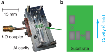
Фигура 4.1: Sample and chip layout. a, Photograph of Darkmon chip ($2.9\times 7$ mm, sapphire) in the aluminum (Al) cavity, which serves as the sample holder, shown with upper half removed. Green arrow points to location of the chip. Also visible: input-output (I-O) SMA coupler and frequency tuning screw (right side). b, Not-to-scale schematic representation of the Bright (vertical) and Dark (horizontal) transmon qubits. Vertical blue arrow indicates the orientation of the electric field of the fundamental ($\mathrm{TE}_{\mathrm{101}}$) cavity mode.

Hamiltonian and level diagram.

Under the rotating-wave approximation and in the low-excitation limit, see Sec. 4.1.3, the effective Hamiltonian of the device, consisting of the Dark, Bright, and cavity modes, is energy conserving,

$$\hat{\overline{H}}/\hbar= \omega_{{\rm D}}\hat{n}_{\emph{{\rm D}}}+\hbar\omega_{{\rm B}}\hat{n}_{{\rm B}}+\hbar\omega_{{\rm C}}\hat{n}_{{\rm C}}$$

$$-\frac{1}{2}\alpha_{{\rm D}}\hat{n}_{\emph{{\rm D}}}\left(\hat{n}_{\emph{{\rm D}}}-\hat{1}\right)-\frac{1}{2}\alpha_{{\rm B}}\hat{n}_{{\rm B}}\left(\hat{n}_{{\rm B}}-\hat{1}\right)$$

$$+\chi_{{\rm DB}}\hat{n}_{\emph{{\rm D}}}\hat{n}_{{\rm B}}+\chi_{{\rm DC}}\hat{n}_{\emph{{\rm D}}}\hat{n}_{{\rm C}}+\chi_{{\rm BC}}\hat{n}_{{\rm B}}\hat{n}_{{\rm C}}\,,$$ (4.1)

where $\hat{n}_{{\rm D,B,C}}$ are the Dark, Bright, and cavity photon-number operators, $\alpha_{{\rm D,B}}$ are the Dark and Bright qubit anharmonicities, also referred to as self-Kerr frequencies, $\chi_{{\rm DB}}$ is the dispersive cross-Kerr frequency shift between the Dark and Bright modes, while $\chi_{{\rm DC,BC}}$ are the dispersive shifts between the cavity and the two transmons. The energy level structure of the two-transmon composite system is schematically represented in Fig. 4.2. When the anharmonicities, $\alpha_{{\rm B}}$ and $\alpha_{{\rm D}},$ are relatively large, typically in the range 100 to 300 MHz, see Table 5.1 for device parameters, the level structure becomes sufficiently anharmonic and we can restrict our attention to the manifold of the four lowest energy states, $\left\{\left|gg\right\rangle,\left|eg\right\rangle,\left|ge\right\rangle,\left|ee\right\rangle\right\}$, where the first (second) letter refers to the Dark (Bright) transmon. When the two qubits are uncoupled, $\chi_{{\rm DB}}=0$, the transitions among the levels contain degeneracies, and $\left|ge\right\rangle$ and $\left|eg\right\rangle$ cannot be addressed individually. In the limit where the coupling, $\chi_{{\rm DB}}$, is large, in practice, on the order of 100 MHz, the degeneracy is lifted, and the $\left|ge\right\rangle$ and $\left|eg\right\rangle$ states become independent, allowing us to further restrict our attention to the three lowest-lying states. We label $\left|gg\right\rangle$ simply as $\left|\mathrm{G}\right\rangle$, $\left|eg\right\rangle$ as $\left|\mathrm{D}\right\rangle$, and $\left|ge\right\rangle$ as $\left|\mathrm{B}\right\rangle.$ In reference to the protected Dark state, $\left|\mathrm{D}\right\rangle$, which is engineered to be decoupled from the environment and readout cavity, we nickname the device ‘‘Darkmon.’’

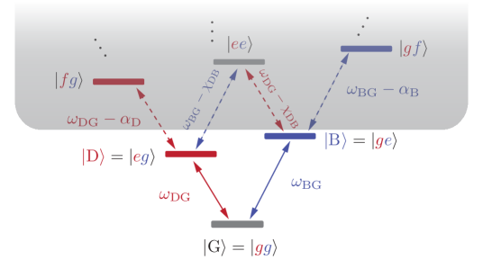
Фигура 4.2: Darkmon energy-level diagram. Energy level diagram of the hybridized Dark and Bright transmon qubits. Red (Blue) color denotes association with the Dark (Bright) transmon, while grey denotes strong association with both transmons. The strong non-linear, dispersive interactions in the circuit, self-Kerr ($\alpha_{{\rm B,D}}$) and cross-Kerr ($\chi_{{\rm DB}}$), allow the lowest-lying three levels to be isolated, and for the two qubit system to be employed as a three-level one with a V-shape structure.

Unique design constraints.

In addition to the required large transmon anharmonicity, $\alpha_{{\rm B}}$, $\alpha_{{\rm D}}$, and cross-Kerr, $\chi_{{\rm DB}},$ frequencies, a few somewhat unique, decoherence related, constraints were required, notably, at odds with the large couplings. First, catching and reversing the quantum jump from $\left|\mathrm{G}\right\rangle$ to $\left|\mathrm{D}\right\rangle$ coherently and with high fidelity required five orders of magnitude in timescales, see Table 5.2, thus imposing the constraint that the $\left|\mathrm{D}\right\rangle$ level coherences be minimally at the $100\ \mathrm{\mu s}$ level, both the energy-relaxation and dephasing times, $T_{1}^{{\rm{\rm D}}},T_{{\rm 2R}}^{{\rm D}}\geq 100\,\mathrm{\mu s}$. The regime of long energy relaxation, $T_{1}^{{\rm{\rm D}}},$ is accessible with the state-of-the-art Purcell-filtered three-dimensional (3D) transmon qubits (Paik et al., 2011, Wang et al., 2015, Dial et al., 2016), but long quantum coherences, $T_{{\rm 2R}}^{{\rm D}}$, are far more difficult to achieve, and are generally obtained by decoupling the transmon qubit from the readout cavity (Gambetta et al., 2006, Rigetti et al., 2012), thus making a tradeoff between quantum coherence and the ability to perform a fast readout. In the quantum jumps experiment, this tradeoff is not permissible, a fast readout of the $\left|\mathrm{D}\right\rangle$ is required simultaneously with long coherences.

To maximize the coherence properties of $\left|\mathrm{D}\right\rangle$, we designed the Dark transmon to be decoupled from all dissipative environments, including the readout cavity and input-output (I-O) coupler. Removing the coupling between $\left|\mathrm{D}\right\rangle$ and the cavity is advantageous in three important ways: it protects $\left|\mathrm{D}\right\rangle$ from i) dephasing due to cavity photon shot noise (Gambetta et al., 2006, Wang et al., 2019, 2018), ii) energy relaxation through the cavity by means of the Purcell effect (Gambetta et al., 2011, Srinivasan et al., 2011, Diniz et al., 2013, Dumur et al., 2015, Novikov et al., 2015, Zhang et al., 2017, Roy et al., 2017), and iii) measurement-induced energy relaxation (Boissonneault et al., 2009, Slichter et al., 2016), see Fig. (5.1). Decoupling $\left|\mathrm{D}\right\rangle$ might seem like a tradeoff at first, since $\left|\mathrm{D}\right\rangle$ can no longer be directly measured through the cavity. However, the strong coupling between the Dark transmon and the Bright transmon, together with the special nature of the V-shape level structure and the $\left|\mathrm{B}\right\rangle$/not-$\left|\mathrm{B}\right\rangle$ dispersive readout, can be employed to nonetheless achieve a fast and faithful readout, see Sec. 5.2.2. The associated challenge is that when two transmon qubits are strongly coupled, the D level needs to remain otherwise isolated and coherent at the same time that the B level is strongly coupled to the low-quality (low-Q) cavity. The coupling between $\left|\mathrm{B}\right\rangle$ and the cavity is necessitated to yield a large dispersive shift, $\chi_{{\rm BC}},$ used to realize the $\left|\mathrm{B}\right\rangle$/not-$\left|\mathrm{B}\right\rangle$ readout; however, this coupling is accompanied by a degree of energy relaxation by means of the Purcell effect inherited by $\left|\mathrm{B}\right\rangle$ (Gambetta et al., 2011). The dissipation in $\left|\mathrm{B}\right\rangle$ can in turn be inherited by the coupled state $\left|\mathrm{D}\right\rangle$, due to the hybridization between the two transmons, $\chi_{{\rm DB}}$, if the design is not carefully optimized.

On a conceptual level, the Darkmon device and the couplings among the levels can be understood in terms of an effective circuit model, see Fig. 4.3, where each mode is represented by a single LC oscillator, with the two qubits having the inductors replaced by non-linear Josephson tunnel junctions. The Dark resonator is capacitively coupled to the Bright one, which is capacitively coupled to the readout resonator, which is capacitively coupled to the input-output transmission line. The Bright and readout resonators can be seen to act as a two-pole filter shielding the Dark resonator from the dissipative effect of the transmission line. While the model is conceptually useful to analyze the qualitative behavior of the circuit, it cannot produce reliable quantitative results. Instead, engineering the highly asymmetric set of couplings while isolating the $\left|\mathrm{D}\right\rangle$ level was achieved by means of an iterative search over the design geometry with the energy participation ratio (EPR) approach. In the following, we briefly summarize the methodology.

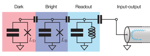
Фигура 4.3: Effective circuit model of Darkmon system. Dark and Bright transmons represented as lumped-element junction-capacitor circuits, junction denoted by cross, coupled an LC circuit representing the readout cavity. $L_{\mathrm{D,B}}$ denote the Dark and Bright Josephson inductances, corresponding to the horizontal and vertical junctions in Fig. 4.1, respectively.

4.1.1 Energy-participation-ratio (EPR) approach

The design of distributed circuits with the aim of obtaining a desired Hamiltonian and set of environmental couplings has attracted a lot of interest (Nigg et al., 2012, Bourassa et al., 2012, Solgun et al., 2014, Solgun and DiVincenzo, 2015, Smith et al., 2016), but a general solution to this inverse problem appears to be out of reach. Instead, one applies a search algorithm over the direct problem — a circuit is chosen, the non-linear mixing and dissipation parameters are calculated, the circuit is modified, and the process is repeated in search of the target parameters. A broadly-applicable approach based on the concept of the energy-participation ratio (EPR) of the nonlinear elements (Josephson devices) in the circuit allows the efficient calculation of the Hamiltonian. In the following, we briefly outline the EPR procedure and finite-element methodology employed in the design of the sample.

Josephson tunnel junction

Non-linear, flux-controlled inductor.

From the point of view of circuit theory (Yurke and Denker, 1984, Devoret, 1997, Girvin, 2014, Vool and Devoret, 2017), a Josephson tunnel junction (Josephson, 1962) is a two-terminal, non-linear, flux-controlled, lumped-element inductor, whose constitutive current-flux relationship is

$$I\left(t\right)=I_{c}\sin\left(\Phi\left(t\right)/\phi_{0}\right)\,,$$ (4.2)

where $I_{c}$ is the critical current of the junction, a phenomenological parameter, $\phi_{0}\equiv\hbar/2e$ is the reduced flux quantum, and $\Phi\left(t\right)$ is the generalized flux across the junction, which has the same dimension as magnetic flux,

$$\Phi\left(t\right)\equiv\int_{-\infty}^{t}\mathrm{d}\tau V\left(\tau\right)\,,$$ (4.3)

where $V$ is the instantaneous voltage drop across the junction terminals. The differential inductance presented by the junction is $L_{J}/\cos\left(\Phi\right),$ where $L_{J}\equiv\phi_{0}/I_{c}$ is known as the Josephson inductance. The quantity $E_{J}\equiv\phi_{0}I_{c}$ is known as the Josephson energy, see Eq. (4.4). Since there are two Josephson junctions in the Darkmon device, we label the junction variables with a subscript $j\in\left\{\mathrm{V,H}\right\}$, where ${\rm V}$ and ${\rm H}$ denote the vertical and horizontal junctions, respectively. From Eq. (4.2) it follows that the potential energy function of the $j$-th junction is a function of flux,

$$\mathcal{E}_{j}\left(\Phi_{j}\right)=E_{j}\left(1-\cos\left(\Phi_{j}/\phi_{0}\right)\right)\,,$$ (4.4)

where $E_{j}$ and $\Phi_{j}$ are the Josephson energy and generalized flux of the $j$-th junction.

Linear and non-linear contributions.

Dropping constant terms, the potential energy of the Josephson junctions, Eq. (4.4), can conceptually be separated in two, corresponding to terms associated with the linear-response and non-linear response of the junction, $\mathcal{E}_{j\mathrm{,lin}}$ and $\mathcal{E}_{j\mathrm{,nl}}$, respectively,

$$\mathcal{E}_{j}\left(\Phi_{j}\right)\equiv\mathcal{E}_{j\mathrm{,lin}}\left(\Phi_{j}\right)+\mathcal{E}_{j\mathrm{,nl}}\left(\Phi_{j}\right)\,,$$ (4.5)

where

$$\mathcal{E}_{j\mathrm{,lin}}\left(\Phi_{j}\right) = \frac{1}{2}E_{j}\left(\frac{\Phi_{j}}{\phi_{0}}\right)^{2}\,,$$ (4.6a)

$$\mathcal{E}_{j\mathrm{,nl}}\left(\Phi_{j}\right) = E_{j}\sum_{p=3}^{\infty}c_{jp}\left(\frac{\Phi_{j}}{\phi_{0}}\right)^{p}\,,$$ (4.6b)

where $c_{jp}$ are the dimensionless coefficients of the Taylor series of $\mathcal{E}_{j}$,

$$c_{jp}=\begin{cases}\frac{\left(-1\right)^{p/2+1}}{p!}&\text{for even }p\\ 0&\text{for odd }p\end{cases}\,.$$ (4.7)

Distributed circuit with non-linear lumped elements

Although electromagnetic (EM) structures are often classified as planar (Blais et al., 2004, Wallraff et al., 2004, Barends et al., 2013, Yan et al., 2016) (2D), quasi-planar (Minev et al., 2013a, 2016, Brecht et al., 2016, Rosenberg et al., 2017) (2.5D), or three-dimensional (Paik et al., 2011, Rigetti et al., 2012, Reagor et al., 2016, Axline et al., 2016) (3D), it is possible to treat these classes on equal footing within the EPR framework. Aside from the junctions, the distributed EM circuit of the readout cavity with the Darkmon chip can be described by a quadratic Hamiltonian function, $\mathcal{H}_{{\rm EM}}$, that depends on the device geometry and the material properties. Analytic treatment of this function is impractical, but finite-element (FE) numerical simulations are adept at handling systems described by quadratic energy functions and finding their eigenmodes (Louisell, 1973, Jin, 2014). The Hamiltonian of the Josephson circuit, consisting of the EM and Josephson elements, is

$$\mathcal{H}=\mathcal{H}_{\mathrm{lin}}+\mathcal{H}_{\mathrm{nl}}\,,$$ (4.8)

where its quadratic part is

$$\mathcal{H}_{\mathrm{lin}}\equiv\mathcal{H}_{{\rm EM}}+\sum_{j\in J}\frac{1}{2}E_{j}\left(\Phi_{j}/\phi_{0}\right)^{2}\,,$$ (4.9)

while its non-linear part, originating from the non-linearity of the Josephson junctions, is

$$\mathcal{H}_{\mathrm{nl}}\equiv\sum_{j\in J}\sum_{p=3}^{\infty}E_{j}c_{jp}\left(\Phi_{j}/\phi_{0}\right)^{p}\,,$$ (4.10)

where, for notational convenience, $J\equiv\left\{\mathrm{V,H}\right\}.$ The quadratic Hamiltonian, $\mathcal{H}_{\mathrm{lin}}$, corresponds to the linearized Josephson circuit (LJC), which can be numerically simulated with FE EM methods to find its eigenfrequencies, $\omega_{m}$, and modal field distributions, consisting of the electric field, $\vec{E}_{m}\left(\vec{r}\right)$, and magnetic field, $\vec{H}_{m}\left(\vec{r}\right)$, eigenvectors over the simulation domain, where $\vec{r}$ is the spatial coordinate. For our device, we restrict our attention to the lowest three eigenmodes, the Dark, Bright, and readout cavity modes, labeled ${\rm D},$ $\mathrm{B}$, and $\mathrm{C}$, respectively; i.e., $m\in M\equiv\left\{\mathrm{D,B,C}\right\}$. Quantizing $\mathcal{H}_{\mathrm{lin}}$, the quantum Hamiltonian of the LJC can thus be expressed

$$\hat{H}_{\mathrm{lin}} =\sum_{m\in M}\hbar\omega_{m}\hat{a}_{m}^{\dagger}\hat{a}_{m}\;,$$ (4.11)

where $\hat{a}_{m}$ is the $m$-th mode amplitude (annihilation operator). Importantly, the frequencies $\omega_{m}$ should be seen as an intermediate parameter entering in the calculation of the rest of the quantum Josephson Hamiltonian,

$$\hat{H}_{\mathrm{nl}} =\sum_{j\in J}\sum_{p=3}^{\infty}E_{j}c_{jp}\hat{\phi}_{j}^{p}\,.$$ (4.12)

While $E_{j}$ and $c_{jp}$ are known from the fabrication of the circuit devices, the quantum operators $\hat{\phi}_{j}\equiv\hat{\Phi}_{j}/\phi_{0}$ remain to be expressed in terms of the mode amplitudes. It can be shown that $\hat{\phi}_{j}$ is a linear combination of the latter,

$$\hat{\phi}_{j}=\sum_{m\in M}\phi_{mj}\left(\hat{a}_{m}^{\dagger}+\hat{a}_{m}\right)\;,$$ (4.13)

where $\phi_{mj}$ are the dimensionless, real-valued zero-point fluctuations (ZPF) of mode $m$ at the position of the junction $j$. Calculation of $\hat{H}$ is now reduced to computing $\phi_{mj}$. We achieve this by employing the energy participation ratio.

Energy participation ratio

We define the EPR $p_{mj}$ of junction $j$ in eigenmode $m$ to be the fraction of the total inductive energy that is stored in the junction,

$$p_{mj} \equiv\frac{\text{Inductive energy stored in junction }j}{\text{Inductive energy stored in mode }m}$$ (4.14a)

$$=\frac{\langle n_{m}|\colon\frac{1}{2}E_{j}\hat{\phi}_{j}^{2}\colon|n_{m}\rangle}{\langle n_{m}|\frac{1}{2}\hat{H}_{\mathrm{lin}}|n_{m}\rangle}\;,$$ (4.14b)

where we have taken the normal-ordered (Gerry and Knight, 2005) expectation values over the state $\left|n_{m}\right\rangle$, a Fock excitation in mode $m$. The normal-ordering, denoted by $\colon\colon$, nulls the parasitic effect of vacuum-energy contributions.

The EPR $p_{mj}$ is computed from the FE eigenfield solutions $\vec{E}_{m}(\vec{r})$ and $\vec{H}_{m}(\vec{r})$ as explained in Sec. 4.1.2. It is a bounded real number, $0\leq p_{mj}\leq 1$. For example, a participation of 0 means that junction $j$ is not excited by mode $m$, while a participation of $1$ means that it is the only inductive element excited by the mode. It can be shown that the values $\phi_{mj}^{2}$ and $p_{mj}$ are directly proportional to each other,

$$\boxed{\phi_{mj}^{2}=p_{mj}\frac{\hbar\omega_{m}}{2E_{j}}\;.}$$ (4.15)

Equation (4.15) constitutes the bridge between the classical solution of the LJC and the quantum Hamiltonian $\hat{H}$ of the full Josephson system, and, as detailed below, is very useful for practical applications.

Fundamental design constraints.

The ZPF $\phi_{mj}$ are not independent of each other, since the EPRs are submitted to three types of constraints. These are of practical importance, as they are useful guides in evaluating the performance of possible designs and assessing their limitations. It is possible to show the EPRs obey one sum rule per junction $j$ and one set of inequalities per mode $m$,

$$\sum_{m\in M}p_{mj}=1 \,,$$ (4.16a)

$$0\leq\sum_{j\in J}p_{mj}\leq 1 \,.$$ (4.16b)

In practice, Eq. (4.16a) can be exploited only if $M$ contains the total number of relevant modes of the system, otherwise the sum of the EPR is bounded by one, rather than equal to one. The final fundamental EPR relation concerns the orthogonality of the EPRs. Solving Eq. (4.15) explicitly for the ZPF,

$$\phi_{mj}=S_{mj}\sqrt{p_{mj}\hbar\omega/2E_{j}}\;,$$ (4.17)

where $S_{mj}=+1$ or $S_{mj}=-1$ is the EPR sign bit of Josephson device $j$ in mode $m$. The EPR sign bit encodes the relative current direction across the Josephson device. Specifically, only the relative value between $S_{mj}$ and $S_{mj^{\prime}}$ for $j\neq j^{\prime}$ has physical significance. The EPR sign bit $S_{mj}$ is calculated during the process of calculating $p_{mj}$, from the field solution $\vec{H}(\vec{r})$, see Eq. (4.25). The EPRs obey the orthogonality relationship

$$\sum_{m\in M}S_{mj}S_{mj^{\prime}}\sqrt{p_{mj}p_{mj^{\prime}}}\, =0\,,$$ (4.18)

valid when all relevant modes are considered.

4.1.2 Calculation of the EPR

Modeling the Josephson junction.

In our device, as in most cQED experiments, the physical dimensions of the Josephson junction ($\approx 10^{-7}$ m) are approximately 5 orders of magnitude smaller than the wavelength of the modes of interest ($\approx 10^{-2}$ m), making the junction geometry unimportant, other than its role in establishing the value of the Josephson inductance $L_{j}$. Similarly, the lead wires leading up to the junction from the transmon pads are deep-sub-wavelength features, and it follows that, typically, their geometry is also unimportant, and can be ignored altogether, aside from any kinetic inductance contribution. In view of this, in the FE simulation, we model the $j$-th junction as a single, two-dimensional rectangular sheet, $S_{j}$, see Fig. 4.4, acting as lumped-element inductor with linear inductance $L_{j}$, Eq. (4.6a). The sheet is assigned a surface-impedance boundary condition that links the tangental electric field, $\vec{E}_{\parallel},$ to the tangental magnetic field, $\vec{H}_{\parallel}$, on the surface of the sheet, $\vec{E}_{\parallel}=Z_{S}(\hat{n}\times\vec{H}_{\parallel}),$ where $\hat{n}$ is the surface normal vector and $Z_{S}$ is the complex surface impedance, which is calculated so that the total sheet inductance is $L_{j}$. Note that in the EM context, a hat symbol denotes a unit vector, not a quantum operator.

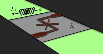
Фигура 4.4: Finite-element model of linearized Josephson junction. Not-to-scale schematic representation of the finite-element model of the linearized Josephson junction (location marked by cross) connected by wire leads (elevated brown trace) to two large metal pads (dark rectangles). Since the geometry of the junction and leads is in deep-sub-wavelength regime, it can typically be ignored, and the inductance presented by the junction, $L_{j}$, graphically represented by black inductor symbol with two open terminals, can be modeled by a single lumped-element inductive sheet, $S_{j}$, in the FE simulation, depicted by light grey rectangle. Green background represents the substrate.

After the design geometry and boundary conditions are established, additional fine-mesh operations on crucial features of interest, such as the junction rectangles, are applied to speed up the solver convergence, which can be diagnosed by examining the parameters $\omega_{m}$ and $p_{mj}$ as a function of adaptive pass number. At each pass, the FE solver provides the modal frequencies, $\omega_{m},$ and the electric, $\vec{E}_{\mathrm{max}}(\vec{r})$, and magnetic, $\vec{H}_{\mathrm{max}}(\vec{r})$, phasors. The electric field at a point $\vec{r}$ in the volume of the device, $V$, at time $t$ is

$$\vec{E}\left(\vec{r},t\right)=\mathrm{Re}\,\vec{E}_{\mathrm{max}}\left(x,y,z\right)e^{j\omega_{m}t}\,.$$

The total magnetic and electric field energies of a mode can be computed from the eigenfields (Pozar, 2011):

$$\mathcal{E}_{\mathrm{elec}} = \frac{1}{4}\mathrm{Re}\int_{V}\mathrm{d}v\vec{E}_{\text{max}}^{*}\overleftrightarrow{\epsilon}\vec{E}_{\text{max}}\;,$$ (4.19)

$$\mathcal{E}_{\mathrm{mag}} = \frac{1}{4}\mathrm{Re}\int_{V}\mathrm{d}v\vec{H}_{\text{max}}^{*}\overleftrightarrow{\mu}\vec{H}_{\text{max}}\;,$$ (4.20)

where the spatial integral is performed over total volume, $V$, of the device, and $\overleftrightarrow{\epsilon}$ ($\overleftrightarrow{\mu}$) is the electric-permittivity (magnetic-permeability) tensor. While the magnetic and electric energies are typically equal on resonance (Pozar, 2011), when lumped elements are included in the model, the more general equality is between the capacitive, $\mathcal{E}_{\mathrm{cap}},$ and inductive, $\mathcal{E}_{\mathrm{ind}},$ energies, $\mathcal{E}_{\mathrm{cap}}=\mathcal{E}_{\mathrm{ind}}\,.$ For our design, the capacitive energy is stored entirely in the electric fields, $\mathcal{E}_{\mathrm{cap}}=\mathcal{E}_{\mathrm{elec}}$, but the inductive energy is stored both in the magnetic fields and in the kinetic inductance of the Josephson junctions, $\mathcal{E}_{\mathrm{mag}}=\mathcal{E}_{\mathrm{ind}}+\mathcal{E}_{\mathrm{kin}}$, where $\mathcal{E}_{\mathrm{kin}}$ is the total energy stored in the kinetic inductors, $\mathcal{H}-\mathcal{H}_{\mathrm{EM}}$, see Eq. (4.9); it follows,

$$\mathcal{E}_{\mathrm{cap}}=\mathcal{E}_{\mathrm{ind}}+\mathcal{E}_{\mathrm{kin}}\,,$$ (4.21)

which, for a single-junction device, implies that the EPR of the junction in mode $m$ is

$$p_{m}=\frac{\mathcal{E}_{\mathrm{elec}}-\mathcal{E}_{\mathrm{mag}}}{\mathcal{E}_{\mathrm{elec}}}\>.$$ (4.22)

For a device with multiple junctions, such as the Darkmon, it follows from Eq. (4.14a), that the EPR of junction $j$ in mode $m$ is

$$p_{mj}=\frac{1}{2}L_{j}I_{mj}{}^{2}/\mathcal{E}_{\mathrm{ind}}\;,$$ (4.23)

where $I_{mj}$ is the junction peak current, which can be calculated from the surface-current density, $\vec{J_{s}^{m}}$, of the junction sheet $S_{j}$,

$$\left|I_{mj}\right|=l_{j}^{-1}\int_{S_{j}}\mathrm{d}s\left|\vec{J_{s}^{m}}\right|\;,$$ (4.24)

where $l_{j}$ is the length of the sheet, see Fig. 4.5.

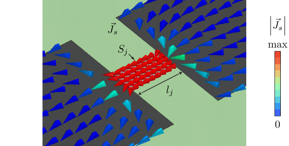
Фигура 4.5: Finite-element simulation of a transmon device. Plot of the surface-current density, $\vec{J}_{S}$, of a transmon qubit mode, obtained with finite-element electromagnetic eigenmode simulation; red (blue) indicates maximum (minimum) current magnitude. Josephson junction (center rectangle) is modeled by a single inductive sheet ($S_{j}$) with length $l_{j}$, spanning the distance between the two transmon pads (dark rectangles). Green background represents the transmon chip.

The calculation of the EPR sign bits, $S_{mj}\in\left\{-1,1\right\}$, requires the definition of a convention for the junction orientation, which is accomplished by supplementing the FE model with a directed line, $\mathrm{DL}_{j}$, along the length of the junction sheet $S_{j}$. The actual orientation of the line is irrelevant, so long as it spans the two terminals of the junction. The sign of the current along the line can be used as the sign bit

$$S_{mj}=\operatorname{sign}\int_{\mathrm{DL}_{j}}\mathrm{d}\vec{l}\cdot\vec{J_{s}^{m}}\;.$$ (4.25)

Remarks.

The convergence of the EPR extracted from local field quantities, $I_{mj},$ can be enhanced by renormalizing the EPRs so as to enforce the global condition given by Eq. (4.21), $\sum_{j\in J}p_{mj}=\mathcal{E}_{\mathrm{kin}}/\mathcal{E}_{\mathrm{ind}}$. The eigenmode simulation approach affords several distinct advantages. No prior knowledge of the mode frequencies is required to execute the simulation. The solver can be queried to solve for the $N$-lowest eigenmodes. If only information on modes above a particular frequency is desired, this cutoff frequency can also be supplied to the solver. From a single mesh and simulation, the FE solver returns complete information for all modes of interest — the parameters $\omega_{m}$, $p_{mj},$ and $S_{mj}$ of the Hamiltonian and, as shown in Sec. 4.1.4, the dissipation budget. These features play nicely into the iterative nature of the design optimization, and make the eigenmode design-optimization process easy to automate, provided freely to the community in our software package pyEPR. In the optimization of the Drakmon device, the finite-element software of choice was Ansys high-frequency electromagnetic-field simulator (HFSS).

4.1.3 Calculation of Hamiltonian parameters with the EPR

The quantities $\omega_{m}$, $p_{mj},$ and $S_{mj}$ obtained from the FE eigenmode solution together with Eqs. (4.13), and (4.15) completely specify $\hat{H}_{\mathrm{nl}}$, Eq. (4.12). The multitude of non-linear interactions contained in $\hat{H}_{\mathrm{nl}}$ mix the LJC modes. However, operating the Darkmon in the dispersive regime (Blais et al., 2004, Koch et al., 2007), defined by $\omega_{k}-\omega_{m}\gg E_{j}c_{jp}\left<\hat{\phi}_{j}^{p}\right>$ for all $p\geq 3$, we can restrict our attention to the leading order correction of $\hat{H}_{\mathrm{nl}}$ to $\hat{H}_{\mathrm{lin}}$ to account for the device spectrum, see level diagram of Fig. 4.2. The leading-order correction is given by the $p=4$ terms that survive the rotating-wave approximation (RWA) (Carmichael, 1999, Gardiner and Zoller, 2004), representing energy-conserving interactions. To leading order, in the RWA, after normal-ordering, $\hat{H}_{\mathrm{nl}}$ reduces to the effective Hamiltonian

$$\hat{\overline{H}}_{4}/\hbar=-\sum_{m\in M}\Delta_{m}\hat{a}_{m}^{\dagger}\hat{a}_{m}+\frac{\alpha_{m}}{2}\hat{a}_{m}^{\dagger 2}\hat{a}_{m}^{2}+\frac{1}{2}\sum_{m\neq n}\chi_{mn}\hat{a}_{m}^{\dagger}\hat{a}_{m}\hat{a}_{n}^{\dagger}\hat{a}_{n}\,,$$ (4.26)

which when combined with $\hat{H}_{\mathrm{lin}}$, Eq. (4.11), yields Eq. (4.1). The Lamb shift, $\Delta_{m}=\frac{1}{2}\sum_{n\in M}\chi_{mn}\,,$ represents the dressing of the linear mode $m$ by the zero-point vacuum energy of all $M$ modes. From Eq. (4.26), it follows that the measured transition frequency between $\left|\mathrm{G}\right\rangle$ and $\left|\mathrm{B}\right\rangle$ is $\omega_{\mathrm{BG}}=\omega_{\mathrm{B}}-\Delta_{\mathrm{B}},$ where $\omega_{\mathrm{B}}$ is the LJC Bright eigenmode frequency and $\Delta_{\mathrm{B}}$ is the Bright mode Lamb shift; a similar conclusion holds for the GD transition. The Kerr frequencies are found from the EPR,

$$\chi_{mn}=-\sum_{j\in J}\frac{\hbar\omega_{m}\omega_{n}}{4E_{j}}p_{mj}p_{nj}$$ (4.27)

and $\alpha_{m}=\chi_{mm}/2$. Remarkably, from Eq. (4.27) it becomes evident that the EPRs are essentially the only free parameters subject to optimization and design in engineering the non-linear couplings, since the frequencies, $\omega_{m}$, and Josephson energies, $E_{j}$, are constrained to a narrow range due to practical considerations. Notably, Eq. (4.27) embodies the structure of a spatial-mode overlap in the EPRs.

4.1.4 Calculation of dissipation budget with the EPR

In this subsection, we summarize the methodology employed in minimizing dissipation in the Darkmon device. This is achieved by optimizing the geometry of the design (in parallel with the Hamiltonian parameter optimization) with the aim of minimizing the susceptibility of each mode to the various unavoidable material and input–output losses. For each design variation, we compute the bound on the modal quality factors by constructing a dissipation budget, which consists of the loss expected due to each lossy element in the design. By manipulating the geometry, the budget can be favorably altered, to a degree. The calculation of the dissipation parameters is detailed in the following.

Losses can be classified as either capacitive, proportional to the electric field intensity, $\left|\vec{E}\right|^{2}$, or inductive, proportional to the magnetic field intensity, $\left|\vec{H}\right|^{2}$. The total loss due to a material is proportional to its energy participation in the mode, $p^{l}$, a geometric quantity related to the field distribution, and its intrinsic quality, $Q$, a material property. The intrinsic material quality, $Q$, can typically only be bounded, while $p^{l}$ can be calculated from the eigenfields. The total capacitive and inductive losses, characterized by $Q_{\text{cap}}$ and $Q_{\text{ind}},$ respectively, sum together with the loss due to input-output coupling, $Q_{\mathrm{rad}}$, and give the upper bound on the quality factor of an EM mode, $Q_{\text{total}}$, (Zmuidzinas, 2012, Geerlings, 2013, Reagor, 2016)

$$\frac{1}{Q_{\text{total}}}=\frac{1}{Q_{\text{cap}}}+\frac{1}{Q_{\text{ind}}}+\frac{1}{Q_{\text{rad}}}\,.$$ (4.28)

In the following, we explicate the calculation of each quantity. We note that the EPR treats dissipation and Hamiltonian parameters on equal footing, and all quantities, Hamiltonian and dissipative, are extracted from a single eigensolution.

Capacitive losses.

Capacitive losses, proportional to the intensity of the electric field, $\left|\vec{E}\right|^{2}$, can originate from bulk or surface of materials. Dielectrics, such as the substrate of the Darkmon device, constitute the primary source of bulk loss (Martinis and Megrant, 2014, Dial et al., 2016, Kamal et al., 2016), and, unfortunately, every surface in a device possesses a near-unavoidable, lossy, surface dielectric layer, possibly due to chemical residues, condensation, dust, etc. (Martinis and Megrant, 2014, Wang et al., 2015). Regardless of the microscopic origin of the dielectric losses, the loss properties of the $l$-th dielectric are characterized by a catch-all quality factor $Q_{\text{cap}}^{l}$ (or equivalently the inverse of the loss tangent) and the EPR of the dielectric in the mode, $p_{\mathrm{cap}}^{l}$ — the fraction of capacitive energy stored in dielectric element $l$. For a bulk dielectric, the dissipative EPR is given by

$$p_{\text{cap,bulk}}^{l}=\frac{1}{\mathcal{E}_{\mathrm{elec}}}\frac{1}{4}\mathrm{Re}\int_{V_{l}}\mathrm{d}v\vec{E}_{\text{max}}^{*}\overleftrightarrow{\epsilon}\vec{E}_{\text{max}}\,,$$ (4.29)

where the integral is carried over the volume of the $l$-th dielectric element, namely $V_{l}$. The dissipative EPR of a surface dielectric, $p_{\mathrm{cap,surf}}^{l}$, can be approximated by

$$p_{\text{cap,surf}}^{l}=\frac{1}{\mathcal{E}_{\mathrm{elec}}}\frac{t_{l}\epsilon_{l}}{4}\mathrm{Re}\int_{\text{surf}_{l}}\mathrm{d}s\left|\vec{E}_{\text{max}}\right|^{2}\,,$$ (4.30)

where the surface layer thickness is $t_{l}$, and its dielectric permittivity is $\epsilon_{l}$. The total capacitive loss in the mode is the EPR-weighted sum of the individual contributions (Zmuidzinas, 2012, Geerlings, 2013),

$$\frac{1}{Q_{\text{cap}}}=\sum_{l}{\frac{p_{\text{cap}}^{l}}{Q_{\text{cap}}^{l}}}\,.$$ (4.31)

Inductive losses.

Electric currents flowing in metals or metal-metal seams can result in inductive losses. The bound on the mode inductive-loss quality factor $Q_{\text{ind}}$ is a weighted sum of the intrinsic material quality $Q_{\text{ind}}^{l}$ of each lossy inductive element $l$, analogous to Eq. (4.31),

$$\frac{1}{Q_{\text{ind}}}=\sum_{l}{\frac{p_{\text{ind}}^{l}}{Q_{\text{ind}}^{l}}}\;,$$ (4.32)

where $p_{\text{ind}}^{l}$ is the inductive-loss EPR of element $l$. For a metal surface, this can be calculated from the eigenfield solutions,

$$p_{\text{ind,surf}}^{l}=\frac{1}{\mathcal{E}_{\mathrm{mag}}}\frac{\lambda_{0}\mu_{l}}{4}\mathrm{Re}\int_{\text{surf}_{l}}\mathrm{d}s\left|\vec{H}_{\text{max},\parallel}\right|^{2}\;,$$ (4.33)

where $\lambda_{0}$ is the metal skin depth at $\omega_{m}$, and $\mu_{l}$ is the magnetic permeability of the surface (typically, $\mu_{l}=\mu_{0}$). In the case of superconductors $p_{\text{ind,surf}}^{l}$ is the kinetic inductance fraction (Gao, 2008, Zmuidzinas, 2012), commonly denoted $\alpha$. Normal metals typically have an inductive quality factor $Q_{\text{ind,surf}}^{l}$ of approximately one (Pozar, 2011). Bulk superconducting aluminum has been measured to have an inductive quality factor $Q_{\text{ind,surf}}$ bounded to be better than a few thousand (Reagor et al., 2013). Meanwhile, the bound on the quality of thin-film Al has been measured to be better than $10^{5}$ (Minev et al., 2013a).

Seam losses.

A distinct loss mechanisms occurs at the seam of two metals (Brecht et al., 2015). For instance, a common source of such loss is the seam used in superconducting cavities. In the FE model, the seam can be modeled by a line, denoted $\text{seam}_{l}$, between the two mating metallic surfaces. The seam inductive participation is

$$p_{\text{ind,seam}}^{l}=\frac{1}{\mathcal{E}_{\mathrm{mag}}}\frac{\lambda_{0}t_{l}\mu_{l}}{4}\mathrm{Re}\int_{\text{seam}_{l}}\mathrm{d}l\left|\vec{H}_{\text{max},\perp}\right|^{2}\;,$$ (4.34)

where the seam thickness is denoted $t_{l}$, its magnetic permeability $\mu_{l}$, and its the penetration depth $\lambda_{0}$. It is convenient to recast the seam loss contribution

$$\frac{p_{\text{ind,seam}}^{l}}{Q_{\text{seam}}}=\frac{1}{g_{\text{seam}}}\frac{\int_{\text{seam}}\left|\vec{J}_{s}\times\vec{l}\right|^{2}dl}{\omega\mu_{0}\int_{\text{vol}}\left|H_{\text{max}}\right|^{2}dV}\;,$$ (4.35)

in terms of a seam admittance $g_{\text{seam}}$, which is defined in Ref. Brecht et al. (2015).

4.2 Sample fabrication

Samples were fabricated on 430 $\mu$m thick, double-side-polished, c-plane sapphire wafers, grown with the edge-defined film-fed growth (EFG) technique, with the bridge-free junction fabrication method, see Refs. Lecocq et al. (2011), Pop et al. (2012), Pop (2011), Reagor (2016). We defined the sample pattern, both large and fine structures, with a 100 kV electron-beam pattern generator (Raith EBPG 5000+) in a single step on a PMAA/MAA resist bilayer. In the following, we describe each step of the fabrication process in detail, and we hope that by adding some additional information about each step and motivation behind it, a reader who is new to the subject will benefit.

Cleaning the wafer.

First, the sapphire wafer is solvent cleaned under a chemical hood in a two-step $N$-Methyl-2-pyrrolidone (NMP) process. The solvent removes dust, organic residues, and oils on the wafer surface. For our samples, we heated the wafer to $90\leavevmode\nobreak\ ^{\circ}\text{C}$ for 10 minutes in an NMP bath, then sonicated it in the bath for another 10 minutes. After removing the wafer from the bath, if it is left out to dry on its own, the NMP would evaporate quickly and leave undesirable residue behind. Instead, we rinsed the wafer in an acetone bath, followed by a methanol one, before finally blow drying it with filtered nitrogen gas. Methanol has low evaporation pressure and under the blow drying tends to take away the residues, rather than simply evaporating and leaving residues behind. An acid should not be used to clean the sapphire wafer, since the wafer is costly and already polished.

Spinning the positive resist bi-layer.

The copolymer resist (Microchem EL-13) is spun onto the cleaned wafer at 2,000 revolutions per minute (r.p.m.) for 100 seconds, then, it is baked for 5 minutes at $200\leavevmode\nobreak\ ^{\circ}\text{C}$. The PMMA resist (Microchem A-4) is spun on top of the first at 2000 r.p.m. for 100 seconds. The wafer is baked at $200\leavevmode\nobreak\ ^{\circ}\text{C}$ for 15 minutes, yielding a thickness of about 200 nm. It is worth noting why PMMA is the resist of choice: it offers high, nm-sized resolution, simplicity and ease of handling, no sensitivity to white light, nor shelf or film life issues, and is easily dissolved, qualities that make it the ideal resist for this type of nanofabrication.

Before proceeding to patterning, fabrication on sapphire requires an extra step: the anti-charging layer. Whereas most silicon substrates are conducive enough to prevent electron beam deflection during the e-beam writing, sapphire substrates are not. The buildup of charge is mitigated by depositing a thin (10 nm) anti-charging layer of gold on the wafer. In terms of metals, gold is an excellent choice, as it is inert, does not have an oxide, and has notably high electrical conductivity. Alternatively, we have also used aluminum for the anti-charging layer (13 nm thick).

Writing and developing the pattern.

Both large and fine structures, including the Josephson tunnel junction are patterned in a single step with the 100 kV EBPG, following which, the gold layer is removed by submerging the wafer in a potassium-iodide/iodine etch solution for 10 seconds. Next, the wafer is rinsed in water and the resist is developed in a 3:1 IPA:water mixture at $6\leavevmode\nobreak\ ^{\circ}\text{C}$ for 2 minutes. After development, the pattern is inspected under an optical microscope.

Plasma cleaning, deposition, and oxidation.

The wafer is loaded in the electron-beam evaporation system, a multi-chamber Plassys UMS300 UHV. To prepare the surfaces for deposition and reduce the amount of aging of the Josephson junction, the exposed sample surfaces are subjected to a 1 minute of oxygen-argon plasma cleaning, under a pressure of $3\times 10^{-3}$ mbar. In this procedure, the etch removed 30 nm from the upper resist layer; however, ideally, one would use a shorter duration and larger pressure (Pop et al., 2012), which was not available. Next, the sample is transferred from the load-lock to the deposition chamber, where an automated titanium sweep is performed to absorb residual gases in the deposition chamber. At an angle of $19$ degrees, 20 nm of Aluminum is deposited onto the sample, following which, the sample is transferred to the oxidation chamber, where it is exposed to a 3:17 oxygen:argon mixture for 10 minutes at 100 Torr. This forms an approximately 1 nm thick aluminum oxide layer, the insulating barrier of the Al/Al$\mathrm{O}_{\mathrm{x}}$/Al Josephson tunnel junctions. The sample is returned to the deposition chamber, where the second and final layer of aluminum (30 nm) is deposited at an angle of $-19$ degrees. Next, rather than directly removing the sample from the evaporation system and allowing the exposed aluminum surfaces to uncontrollably oxidize in air, the surfaces are passivated with a final oxidation step at 50 Torr for 10 minutes. The aluminum forms a self-limiting oxide capping layer.

Liftoff.

The sample is placed in a heated bath of NMP solvent at $70\leavevmode\nobreak\ ^{\circ}\text{C}$ for two hours. It is then sonicated for 1 minute, while still in the NMP, following which, the NMP is cleaned with acetone, methanol, IPA, and, finally, a dry nitrogen blow gun. The solvent ‘‘lifts off’’ the unwanted metal from the wafer by dissolving the resist underneath it, thus leaving the bath full of aluminum flakes. Note that NMP can’t be heated much above $100\leavevmode\nobreak\ ^{\circ}\text{C}$, since that will likely damage the Al/Al$\mathrm{O}_{\mathrm{x}}$/Al junctions.

Dicing.

A protective coating of optical resist (SC1827) is spun at 1,500 r.p.m. for 120 seconds and baked at $90\leavevmode\nobreak\ ^{\circ}\text{C}$ for 5 minutes. The sample is loaded in the dicer (ADT ProVecturs 7100), which then is calibrated, aligned, and which then performs the dicing. The diced chips are cleaned with acetone, methanol, and dry nitrogen, and are stored until they ready to be mounted in the sample holder.

Sample selection.

The diced chips are cleaned (NMP, Acetone, methanol, nitrogen air) and visually examined under an optical microscope where the normal-state resistance, $R_{N}$, of their Josephson junctions is measured. This is performed under an optical microscope (Copra Optical Inc. SMZ800) with probe needles (Quater-Research H-20242) lowered to contact the transmon pads on either side of the junction, taking care to properly ground all object in contact with the sample and to minimize unavoidable scratching of the pad during the probing. The measurement of $R_{N}$ provides a good estimate of the junction Josephson energy, $E_{J}$, by an extrapolation from room temperature to the operating sample temperature, at approximately $15$ mK, using the Ambegaokar-Baratoff relation (Ambegaokar and Baratoff, 1963),

$$E_{J}=\frac{1}{2}\frac{h\Delta}{\left(2e\right)^{2}}R_{N}^{-1},$$ (4.36)

where $\Delta$ is the superconducting gap of aluminum. The chip closest matching the Josephson energies, $E_{J}$, of the EPR-designed vertical and horizontal junctions is selected for mounting in the sample holder.

4.3 Sample holder

In this section, we describe the methodology used in the design of the sample holder and readout cavity, while paying special attention to the motivation underlying the design choices. The boundary conditions of the readout cavity, depicted in Fig. 1.1, are formed from the superconducting inner walls of the chip sample holder, composed of two main halves, see Fig. 4.6c, and based on the ideas presented in Ref. Paik et al. (2011). Before a discussion on the design geometry, we focus on the selection of its materials.

4.3.1 Material losses and selection

Readout cavity considerations.

The inner walls of the sample holder establish the boundary conditions of the readout cavity mode, and hence have a large inductive, $p_{\text{ind,surf}}^{l}$, and dielectric, $p_{\text{cap,surf}}^{l},$ surface-loss participation ratio, see Sec. 4.1.4. It follows that the material quality of the cavity inner walls is important in determining the readout quality factor, $Q_{\mathrm{R}}$. However, since this mode is purposefully made low-Q, by coupling it strongly to the input-output (I-O) couplers, the importance of the sample-wall material is greatly reduced, and could in principle be rather lossy. For instance, in some designs, copper, which has an inductive quality factor of unity, $Q=1$, has been used, thus limiting $Q_{\mathrm{R}}$ to several thousand. Under these conditions, a fraction of the readout cavity signal is lost to the walls of the cavity, rather than to the I-O couplers. Nonetheless, the I-O coupling is engineered to be larger still, so that most of the signal in the readout cavity makes it to the amplifier chain, and a high quantum measurement efficiency, $\eta$, can still be obtained.

Qubit mode considerations.

However, the Bright and Dark qubit modes, while predominantly spatially localized to the sapphire substrate region, have a small fraction of their fields extending to the inner walls of the readout cavity. Although the lossy energy participation ratios, $p_{\text{ind,surf}}^{l}$ and $p_{\text{cap,surf}}^{l}$, are exponentially small ($\lesssim 10^{-5}$), so that the cavity walls participate on the part-per-million level, a normal-metal wall ($Q_{\mathrm{ind}}^{l}\approx 1$) could limit the qubit quality factors significantly, making lifetimes on the order of $T_{\mathrm{1}}^{\mathrm{D}}\approx 100\ \mathrm{\mu s}$ out of reach. For this reason, we employ a low-loss superconducting material for the sample holder, and clean its surfaces with care, see discussion on Pg. 4.4.2. Specifically, we machined the readout cavity from 6061 aluminum alloy, which is typically found in the construction of aircraft structures. Notably, it is a good superconductor, and due to its hardened structure offers a machining advantage over regular aluminum, which is too soft.

We remark that in other experiments, involving high-Q storage mode cavities, the cavities are often machined from high-purity 4N (99.99% pure) aluminum (or sometimes, 5N), which is very soft, and thus difficult to machine. Further, the machining forms deep cracks ($\approx 100\ \mathrm{\mu m}$), where machining oils and dirt seep in, and hence, the surfaces require a more involved chemical etch process to remove about 150$\ \mathrm{\mu}$m of the surface; see the dissertation of M. Reagor (Reagor, 2016).

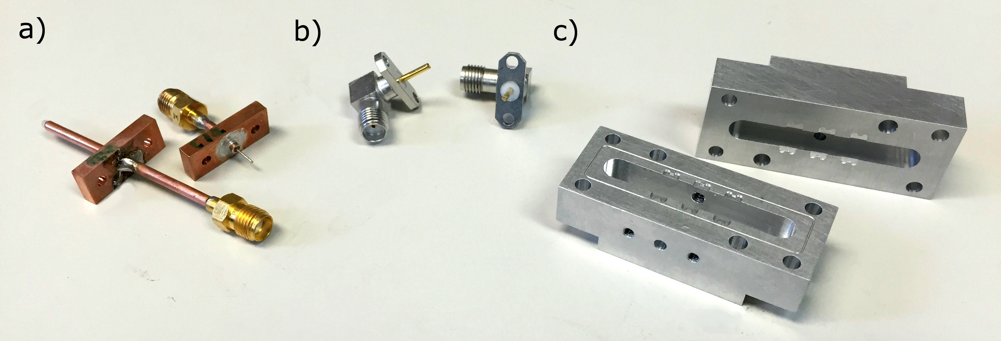
Фигура 4.6: Non-magnetic couplers and sampler holder. a/b, Photograph of two generations of custom-made, non-magnetic, SubMiniature version A (SMA), input-output (I-O) pin couplers. c, Photograph of disassembled sample holder, inside walls forms boundary condition for the readout cavity mode. Three machined grooves on the mating surfaces of the two halves provide placement slots for samples. Mating surface of lower-half has groove encircling the inside cavity, employed with an indium wire to seal the two halves. Large through holes visible on the mating surfaces provide means to fasten sample holder and attach it to a cold finger in the dilution refrigerator. Small hole visible on the interior back wall of the lower half allows for screw-tuning of the readout cavity frequency.

Non-magnetic input-output couplers.

It has been recognized that commercial flange-based I-O couplers contain magnetic ferrite impurities with fields at the ten milligauss level, which although small, due to the close spatial proximity of the coupler to the thin-film superconducting pads of the transmon, as well as the Josephson junction, could introduce vortices in the films, and it is suspected, generally degrade the superconductor performance. To achieve better control of the electromagnetic environment and to reduce potential losses due to magnetic impurities, we employed custom-made pins from non-magnetic materials, such as copper and brass.

Panels (a) and (b) of Fig. 4.6 show two generations of non-magnetic, SubMiniature version A (SMA) pin-couplers. The first generation, see panel (a), was made in-house from a standard, SMA copper cable with two female connectors. After testing the quality of the cable, by checking its insertion loss with a vector network analyzer (VNA), the cable was cut in two, partially stripped (external shielding and teflon) to expose the center conductor, which serves as the pin inside the readout cavity, and soldered (non-magnetic solder) to a custom copper flange. The flange can then be mounted to the outside surface of the readout cavity, see panel (c), by non-magnetic, brass or aluminum, screws. Panel (b) shows a second generation of non-magnetic couplers, made from beryllium-copper, and custom-ordered, courtesy of Christopher Axline. In general, components used with the sample holder, placed inside the enclosing magnetic shielding, were tested for magnetic compatibility with a magnetometer inside a magnetically shielded box at room-temperature.

Sample-holder seam.

To enclose the Darkmon chip in the sample holder, the sample holder is designed as two separate halves, see Fig. 4.6c. As discussed in Sec. 4.1.4, the placement of the seam in the design is important, as it determines the seam-loss participation ratio, $p_{\text{ind,seam}}^{l}$. The seam in placed at the minimum of the current field profile of the readout cavity mode. No perfect symmetry exists in the design; it is broken by the I-O couplers and the sample chip, so even at this location, the participation is not strictly zero for either the readout cavity or qubit modes. For this reason, it is important that the seam quality is as high as possible. In the following, we remark on seam properties at the microscopic level, and the use of an indium seal for improved electrical contact.

Seam quality at the microscopic level. Even under high pressure, applied by the fastening action of the sample holder screws, see Fig. 4.6c, the mating faces of the two halves of the sample holder do not join well at the atomic level. Three interface regions can be identified: i) metal-to-metal regions, the rarest, where aluminum atoms from both halves are in physical contact, allowing superconducting current to flow undisturbed, ii) semi-conducting regions, more common, where contaminants, typically dielectric, result in resistive conductance, and iii) non-conducting regions, typically, the most common, where electrical flow is altogether prohibited, for either the region is a vacuum gap or is dominated by a thick non-conductive film of oxides, sulphides, etc. The physical contact area is typically less than a tenth of the area of the mating surfaces.

Higher-quality seam. To create a seam with higher electrical conductivity, one can first increase the force applied to form the bond to fracture the native oxide layer of the mating surfaces and to yield a greater physical contact area, region (i). However, this method is rather limited in applicability with our design, because the constraint of non-magnetic screws excludes nearly all hard-material screws, including stainless steel ones, due to magnetic impurities. The soft screws we use, aluminum and brass, lack the impurities needed to make them withstand larger forces, and tend to break and strip easily. Mostly, we relied on a soft-metal seal, a thin wire gasket placed in a small groove in one of the mating faces. A number of materials metals are conventionally used as soft-metal seals, such as copper, aluminum, indium, etc. The seal of choice in the cQED community is indium, typically used in cryogenic hermetic seals and low-temperature solder with melting point of 47 °C, since it remains soft and malleable even at cryogenic temperatures and is a superconductor. The indium gasket has been observed to increase the internal quality factor of a superconducting cavity by several orders of magnitude and its estimated seam conductance is $g_{\mathrm{seam}}\gtrsim 10^{6}/\mathrm{\Omega m}$ (Brecht, 2017). In our experiment, we used an un-greased 99.99% indium wire of 0.020 in. diameter to form the seam gasket.

4.3.2 Assembly

After the surfaces of the machined sample holder are cleaned, see discussion on Pg. 4.4.2, the Darkmon chip selected from the diced wafer, Sec. 4.2, is cleaned (NMP, Acetone, methanol, nitrogen air) and, under an optical microscope, is immediately placed in the central groove of the sample holder, see Fig. 4.1a. The groove is designed to be larger (at minimum 5%) than the dimensions of the chip to account for the differential thermal contraction between aluminum and sapphire (mostly, the aluminum contracts) and machining tolerances. The precision of the dicing saw (ADT ProVecturs 7100) is high, several microns when recently calibrated, and the chip will not exceed the diced margin by more than a few microns, but it can fall quite short of that, because, unlike silicon, when sapphire is diced, it shatters around the edges, much like glass, and forms a jagged edge. For this reason, when placed in the groove, the chip can rattle about, and requires anchoring, accomplished by placing four small bits of indium on its four corners and pressing them down to fill the corner circular pockets machined in the groove, see Fig. 4.6c. To minimize contamination during the mounting, the chip is placed face down in the groove, although, we note that even dust on the back side of the chip can contribute to loss in the qubit modes, though, its participation ratio will be far smaller than if it were on the front face.

When the sample is well anchored, the indium gasket is laid down in the gasket groove, as visible in Fig. 4.1a, and the top half of the sample holder is mounted on top, fastened tightly with even-pressure to allow the indium to distribute evenly. For the screws, we used aircraft-alloy 7075 (McMaster/Fastener Express), with less than 1% iron impurities. These screws, as discussed earlier, are rather soft, and to achieve a higher compression between the two halves at cryogenic temperatures, we used the screws with molybdenum washers, which provide differential contraction — the linear thermal contraction for molybdenum (aluminum) between room temperature and 4 K is 0.095% (0.415%). Molybdenum is compatible with the non-magnetic requirement. After 10 minutes, the indium seal relaxes, and the screws can be further tightened, with even pressure.

4.4 Cryogenic setup

The embedding environment of the sample is nearly as important as the properties of the sample itself in achieving long-coherences and desired performance. For this reason, in this section, we focus on a few notable aspects of the cryogenic setup, and pay particular attention to motivations. For the most part, our cryogenic setup is rather standard in the field of cQED. For a more general discussion of low-temperature cryogenics, see Refs. Ventura and Risegari (2010) and Pobell (2013).

4.4.1 Material selection

As already emphasized, the material selection of components used in the setup is of prime importance. For this reason, we feel it worthwhile to note a few overriding principles, corroborated by experience, employed when selecting materials for the cryogenic setup of a cQED experiment, which have to be compatible with operation at milikelvin temperatures and high vacuum ($<10^{-1}$  Pa).

Tested and well-understood cryogenic materials.

In the cryogenic setup of our experiment, we employed only materials that have been exhaustively studied, characterized, and established in regular laboratory use. There are only a handful suitable for cQED experiments, which, in the solid-state, can classified as: i) ambient-pressure superconductors: aluminum, niobium, indium, titanium, tin, molybdenum, and niobium-titanium (NbTi), ii) normal metals: copper, brass, gold, beryllium, stainless steel, and iii) dielectrics: silicon, sapphire, quartz, nylon, Teflon, Stycast, poly(methyl methacrylate) (PMMA). The listed materials are the most common ones; for material properties, see Refs. Ventura and Risegari (2010) and Pobell (2013).

Simplicity and homogeneity.

The simplest and smallest number of materials were employed in the cryogenic setup. The Darkmon sample (including I-O pins, seam gaskets, screws, et cetera) consisted of essentially three types of atoms — aluminum, oxygen, and indium. Beyond the materials employed in the sample holder, the properties of commercial components were found to vary among manufacturers, for instance, the residual magnetic impurity levels measured in screws and SMA connectors, barrels, adapters, et cetera varied across manufacturers. For this reason, prior to use in the setup, all components were screened with a magnetometer, especially when employed inside magnetically shielded compartments.

Aluminum.

Chief among the materials employed was aluminum (Al), and hence, we pay special attention to its properties. From a structural standpoint, Al is ‘‘light-weight,’’ having one-third the density and stiffness of steel and copper. However, unlike steel, it is free of magnetic impurities and has 59% of the thermal and electrical conductivity of copper at room temperature. Importantly, when aluminum oxidizes, it forms a protective coating of amorphous aluminum oxide ($\mathrm{AlO_{x}}$) that is thermodynamically favored to self limit growth to a thickness of merely one nanometer. The $\mathrm{AlO_{x}}$ layer is special in that it has one of the highest hardness coefficients of all oxides, even greater than glass, making it an excellent (unavoidable) encapsulation layer, rendering Al highly resistant to corrosion, but also making the formation of a very-conductive Al-Al seam difficult, as discussed on Pg. 4.3.1, and resulting in a surface dielectric layer with a loss tangent, see Sec. 4.1.4.

4.4.2 Thermalization

The design and implementation of a high-thermal-conductivity link between the Darkmon sample and the main source of cooling power in the dilution refrigerator, the mixing chamber pot, is crucial to take undesired heat away from the sample. At low temperatures, the task is complicated since the rate limiting factor in the heat transfer becomes the contact thermal resistance, $R_{\mathrm{C}},$ found at the interface of two mating surfaces, intricately dependent upon on the interface properties and difficult to control. The temperature discontinuity, $\Delta T$, across two mating surfaces is

$$\Delta T=\frac{R_{\mathrm{C}}}{A}\dot{Q}\,,$$ (4.37)

where $A$ is the surface area and $\dot{Q}$ is the power flowing through the surface. It is seen that to minimize $\Delta T$ once can increase the contact area, $A$, or decrease the geometry-independent resistance, $R_{\mathrm{C}}.$ In the following, we describe the thermal link setup of the sample and briefly outline the strategies employed to minimize $R_{C}$ across the various interfaces.

Gold plating and welding. The sample was mounted on a cold-finger attached to the mezzanine mixing-chamber plate. The plate is gold plated ($\approx 5\mu m$ by electroplating) to achieve higher thermal conductivity. As a soft metal, gold allows for a larger ’real’ surface-area contact, and due to its chemical inertness, also provides protection from oxidation of the surface, which keeps $R_{\mathrm{C}}$ low across multiple uses and over time. The cold finger is not gold-plated, due to the cost and long-lead time of the process. It is machined from two oxygen-free high-thermal-conductivity (OFHC) copper blocks, which are welded together to minimize the number of contact joints, essentially eliminating $R_{\mathrm{C}}$ altogether. Of course, the bulk thermal resistance of the OFHC copper block remains, but it is rather small and the cross-sectional area of the cold-finger block is rather large, providing a good thermal link.

Pressure and differential contraction. The sample is fixed to the cold finger with aluminum screws. The cold finger is mounted on the mezzanine mixing-chamber plate with stainless steel screws, which allow greater pressure. To maximize the pressure across all joints, molybdenum washers were used everywhere to provide further differential-contraction pressure, see discussion on Pg. 4.3.2.

Thermal straps. The cold finger thermalization link contains several unavoidable joins, an issue that can be circumvented to a degree with the use of a flexible heat strap (also known as thermal braid). Directly mounted on the sample was a small copper block welded to a thick OFHC copper heat strap (models P6-501 and P7-501 from TAI) that extended to the mixing chamber plate without interruption. The strap has the advantage of being durable, flexible, and reusable.

Surface preparation. The physical and chemical condition of the surfaces forming the contact determine $R_{\mathrm{C}}$. When a component is machined, the stresses applied to the surface create dislocations and riddle the surface with extremely narrow (order of a few nanometers) but deep (hundreds of nanometers) cracks, into which machining oils seep. The cracks and oil residues degrade the surface quality, visually, electrically, and thermally. For this reason, all surfaces involved in forming a thermal link were prepared in the following way. First, they were cleaned abrasively with scotch bright, buffing, and fine sandpaper, removing the top surface layer and resulting in a shiny mirror finish. Second, the mating component was cleaned chemically. Typically, by sonication in an anionic detergent solution (Alconox 1%), followed by acetone, then IPA, and finally blow dried with dry nitrogen air. For more aggressive cleaning, we used a powerful oxidizing agent, nitric acid ($\mathrm{HNO_{3}}$), to etch the surface. The acid and oxidized impurities were then washed away with deionized water, followed by an acetone and isopropanol (IPA) bath, and finally a nitrogen blow dry. The components were then mounted immediately, before a substantial oxide layer could form. For previously treated components that required remounting, the mating surface was cleaned with blue solder flux, which has a high concentration of nitric acid, immediately prior to mounting.

4.4.3 Light and magnetic shielding

The quality factor of superconducting microwave aluminum resonators (and qubits) is known to strongly depend on the quality of the infrared and magnetic shielding of the embedding environment (Barends et al., 2011, Wang et al., 2014, Kreikebaum et al., 2016). Stray infrared light that is absorbed by a superconductor creates quasiparticles, which reduces the overall quality factor of the superconducting surface. This effect is especially pronounced in aluminum, whose superconducting gap is rather low, $\approx 88$ GHz (Barends et al., 2011, de Visser et al., 2011). The effect of stray light can be largely mitigated with multistage infrared shielding. Magnetic fields at the surface of the superconductor can suppress the superconducting gap and introduce vortices, which generally reduce the inductive surface quality, although, under certain conditions, the vortices can act as quasiparticle traps, and can result in overall higher quality (Wang et al., 2014, Vool et al., 2014).

Light shielding.

Black-body radiation from warmer stages in the dilution refrigerator was blocked by reflective thermal shields enclosing the mixing chamber space and special care with taken to prevent line-of-sight leaks through screw holes, et cetera. However, low frequency photons are more difficult to shield against, and several further strategies were employed to make a light-tight sample space for the Darkmon device. In addition to the indium seal between the two metal halves of the sample holder, the sample holder was wrapped in three layers of aluminized mylar foil, secured with copper tape. In some cooldowns, the inside of the magnetic shield housing the sample (see below) was lined with infrared absorbing epoxy (Barends et al., 2011, Rigetti et al., 2012). Coaxial thermalization and infrared filters (teflon replaced by Eccosorb CR-110 as the dielectric) were used on the input and output lines of the sample.

Magnetic shielding.

A high-magnetic-permeability, $\mu$-metal (Amumetal A4K) can enclosed an aluminum superconducting cylinder which housed the sample. In this configuration, the $\mu$-metal shield allows the superconducting shield to cool through its critical temperature in a lower magnetic field, lowering the possibility of vortex trapping. Both shields were thermally anchored to the mixing-chamber base plate by thermal straps, while the $\mu$-metal shield was also anchored to the cold-finger by direct contact. Components employed within the can were tested for magnetic impurities with a magnetometer. Special care was taken to avoid markings and paint that could be magnetic; paint on components, such as directional couplers, was stripped with a solvent bath (typically, Acetone).

4.5 Microwave setup

Room temperature.

The control tones depicted in Fig. 1.1 were each generated from individual microwave generators ($\Omega_{\mathrm{D}}$ and $\Omega_{\mathrm{B0}}$: Agilent N5183A; readout cavity tone R and $\Omega_{\mathrm{B1}}$: Vaunix LabBrick LMS-103-13 and LMS-802-13, respectively). To achieve IQ control, the generated tones were mixed (Marki Microwave Mixers IQ-0618LXP for the cavity and IQ-0307LXP for $\Omega_{\mathrm{B0}},\Omega_{\mathrm{B1}}$, and $\Omega_{\mathrm{D}}$) with intermediate-frequency (IF) signals synthesized by the 16 bit digital-to-analog converters (DACs) of the integrated FPGA controller system (Innovative Integration VPXI-ePC). Prior to mixing, each analog output was filtered by a $50\,\Omega$ low pass filter (Mini-Circuits BLP-300+) and attenuated by a minimum of 10 dB. The radio-frequency (RF) output was amplified at room temperature (MiniCircuits ZVA-183-S+) and filtered by Mini-Circuits coaxial bandpass filters. The output signal was further pulse modulated by the FPGA with high-isolation SPST switches (Analog Device HMC-C019), which provided additional 80 dB isolation when the control drives were turned off. The signals were subsequently routed to the input lines of the refrigerator.

At room temperature, following the cryogenic high-electron mobility amplifier (HEMT; Low Noise Factory LNF-LNC7_10A), the signal were amplified by 28 dB (Miteq AFS3-00101200-35-ULN) before being mixed down (Marki image reject double-balanced mixer IRW-0618) to an intermediate frequency (IF) of 50 MHz, where they were band-pass filtered (Mini-Circuits SIF-50+) and further amplified by a cascaded preamplifier (Stanford Research Systems SR445A), before finally digitization by the FPGA analog-to-digital converters (ADC).

Cryogenic.

The experiments were carried out in a cryogen-free dilution refrigerator (Oxford Triton 200). Our input-output cryogenic setup is nearly identical to that described in Ofek et al. (2016) and Minev et al. (2016), aside from the differences evident in the schematic of our setup (see Figs. 1.1b) Notably, for the output lines between the sample and the HEMT, we employed low-loss superconducting cables (CoaxCo Ltd. SC-086/50-NbTi-NbTi PTFE). The input line had a 12 GHz low-pass filter (K&L 6L250-12000/T26000-OP/O) and the output line had two broadband isolators (Quinstar CWJ1019-K414), providing a total of 36 dB of reverse isolation between the HEMT and the JPC. Since the experiment spanned more than a dozen cool-downs, we note that regular retightening of all cryogenic SMA connectors and screws was observed to yield overall better performance.

5Additional experimental results

A strong claim of violation [of Bell’s inequality] should be supported by at least a 5 sigma deviation.

Alain Aspect
Rosenthal Lecture, 2018

This chapter presents experimental results and control experiments that support the main experimental results and conclusions presented in Chapter 1. The characterization of the Hamiltonian parameters, coherence properties, and other non-idealities of the two-transmon, one-readout-cavity device employed in the experiment is discussed in Sec. 5.1. The calibration of the tomography and control pulses and relevant control experiments are discussed in Sec. 5.2. A summary of the drive amplitudes and frequencies can be found in Sec. 5.2.3. Details of the experimental flow of the catch and reverse protocol with regard to the FPGA controller are discussed in Sec. 5.4. A comparison between the predictions of the quantum trajectory description of the experiment developed in Chapter 3 and the main experimental results is presented in Sec. 5.5.

5.1 Characterization of the system

In this section, we describe the characterization of the Hamiltonian and coherence parameters of the two-transmon, one-readout-cavity device employed in the experiment. In reference to the protected Dark level, which is engineered to be decoupled from the environment and readout cavity, we nickname the device ‘‘Darkmon.’’ The low-excitation manifold of the Darkmon device is well described by the approximate dispersive Hamiltonian, see Sec. 4.1,

$$\hat{H}/\hbar= \omega_{\mathrm{B}}\hat{b}^{\dagger}\hat{b}-\frac{1}{2}\alpha_{\mathrm{B}}\hat{b}^{\dagger 2}\hat{b}^{2}+\omega_{\mathrm{D}}\hat{d}^{\dagger}\hat{d}-\frac{1}{2}\alpha_{\mathrm{D}}\hat{d}^{\dagger 2}\hat{d}^{2}-\chi_{\mathrm{DB}}\hat{b}^{\dagger}\hat{b}\hat{d}^{\dagger}\hat{d}$$ (5.1)

$$\left(\omega_{\mathrm{C}}+\chi_{\mathrm{B}}\hat{b}^{\dagger}\hat{b}+\chi_{\mathrm{D}}\hat{d}^{\dagger}\hat{d}\right)\hat{c}^{\dagger}\hat{c}\,,$$

where $\omega_{\mathrm{D,B,C}}$ are the Dark, Bright, and cavity mode frequencies, $\hat{d}$, $\hat{b},$ $\hat{c}$ are the respective mode amplitude (annihilation) operators, $\alpha_{{\rm D}}$ ($\alpha_{{\rm B}}$) is the Dark (Bright) transmon anharmonicity, $\chi_{\mathrm{D}}$ ($\chi_{\mathrm{B}}$) is the dispersive shift between the Dark (Bright) transmon and the readout cavity, and $\chi_{\mathrm{DB}}$ is the dispersive shift between the two qubits. The Dark, $\left|\mathrm{D}\right\rangle$, and Bright, $\left|\mathrm{B}\right\rangle,$ states correspond to a single excitation in the Dark and Bright transmon modes, $\hat{d}^{\dagger}\left|0\right\rangle$ and $\hat{b}^{\dagger}\left|0\right\rangle$, respectively; see Fig. 4.2 for a level diagram of the low-energy manifold.

The readout cavity frequency was spectroscopically measured in reflection (Geerlings, 2013), $\omega_{\mathrm{C}}/2\pi=8979.640\text{\,MHz}$, and the extracted cavity linewidth agreed well with an independent measurement of the energy-relaxation rate of the cavity extracted from a time-domain ring-down measurement, $\kappa/2\pi=3.62\pm 0.05\,\mathrm{MHz}.$ The cavity was observed to be well over-coupled; i.e., the coupling quality factor, $Q_{c}$, dominated the internal quality factor, $Q_{i}$; making it difficult to precisely extract $Q_{i}.$ The frequency and anharmonicity of the B transmon were $\omega_{\mathrm{B}}/2\pi=5570.349\,\mathrm{MHz}$ and $\alpha_{\mathrm{B}}/2\pi=195\,\mathrm{MHz}$, respectively, measured with two-tone pulsed spectroscopy (Geerlings, 2013, Reagor, 2016). The frequency and anharmonicity of the D transmon, $\omega_{\mathrm{D}}/2\pi=4845.255\,\mathrm{MHz}$ and $\alpha_{\mathrm{D}}/2\pi=152\,\mathrm{MHz}$, respectively, were measured in a modified two-tone spectroscopy sequence, where the $\left|\mathrm{G}\right\rangle$ level was mapped to the $\left|\mathrm{B}\right\rangle$ level at the end of the spectroscopy sequence, before the readout, with $\pi$-pulse on the BG transition. In a similar two-tone spectroscopy experiment, which included a pre-rotation on either the BG or DG transition, and a measurement rotation after the probe tone is turned off but before the readout tone is actuated, the cross-Kerr coupling between the two qubits was measured to be $\chi_{\mathrm{DB}}/2\pi=61\pm 2\,\mathrm{MHz}$. In a standard energy-relaxation experiment (Geerlings, 2013), the $\left|\mathrm{B}\right\rangle$ lifetime was measured to be $T_{\mathrm{1}}^{\mathrm{B}}=28\pm 2\,\mathrm{\mu s}$, which we believe is limited by the Purcell effect with the readout cavity mode, based on a finite-element calculation, see Sec. 4.1.2. The Ramsey coherence time of $\left|\mathrm{B}\right\rangle$ was $T_{\mathrm{2}}^{\mathrm{R,B}}=18\pm 1\,\mathrm{\mu s}$, possibly limited by photon shot noise (Gambetta et al., 2006, Rigetti et al., 2012). The measured Hamiltonian and coherence parameters of the device are summarized in Table 5.1, where the drive parameters employed in the experiment can also be found.

Readout cavity		BG transition		DG transition
Mode frequencies and non-linear parameters
$\omega_{\mathrm{C}}/2\pi=$	$8979.640\text{\,MHz}$	$\omega_{\mathrm{BG}}/2\pi=$	$5570.349\text{\,MHz}$	$\omega_{\mathrm{DG}}/2\pi=$	$4845.255\text{\,MHz}$
		$\chi_{\mathrm{B}}/2\pi=$	$-5.08\pm 0.2\,\mathrm{MHz}$	$\chi_{\mathrm{D}}/2\pi=$	$-0.33\pm 0.08\,\mathrm{MHz}$
		$\alpha_{\mathrm{B}}/2\pi=$	$195\pm 2\,\mathrm{MHz}$	$\alpha_{\mathrm{D}}/2\pi=$	$152\pm 2\,\mathrm{MHz}$
		$\chi_{\mathrm{DB}}/2\pi=61\pm 2\,\mathrm{MHz}$
Coherence related parameters
$\kappa/2\pi$=	$3.62\pm 0.05\,\mathrm{MHz}$	$T_{\mathrm{1}}^{\mathrm{B}}=$	$28\pm 2\,\mathrm{\mu s}$	$T_{\mathrm{1}}^{\mathrm{D}}=$	$116\pm 5\,\mathrm{\mu s}$
$\eta=$	$0.33\pm 0.03$	$T_{\mathrm{2\mathrm{R}}}^{\mathrm{B}}=$	$18\pm 1\,\mathrm{\mu s}$	$T_{\mathrm{2\mathrm{R}}}^{\mathrm{D}}=$	$120\pm 5\,\mathrm{\mu s}$
$T_{\mathrm{int}}=$	$260.0\,\mathrm{ns}$	$T_{\mathrm{2\mathrm{E}}}^{\mathrm{B}}=$	$25\pm 2\,\mathrm{\mu s}$	$T_{\mathrm{2\mathrm{E}}}^{\mathrm{D}}=$	$162\pm 6\,\mathrm{\mu s}$
$n_{\mathrm{th}}^{\mathrm{C}}\leq$	$0.0017\pm 0.0002$	$n_{\mathrm{th}}^{\mathrm{B}}\leq$	$0.01\pm 0.005$	$n_{\mathrm{th}}^{\mathrm{D}}\leq$	$0.05\pm 0.01$
Drive amplitude and detuning parameters
$\bar{n}=$	$5.0\pm 0.2$	$\Omega_{\mathrm{B}0}/2\pi=$	$1.20\pm 0.01\,\mathrm{MHz}$	$\Omega_{\mathrm{DG}}/2\pi=$	$20\pm 2\,\mathrm{kHz}$
		$\Omega_{\mathrm{B}1}/2\pi=$	$0.60\pm 0.01\,\mathrm{MHz}$
$\Delta_{\mathrm{R}}=$	$\chi_{\mathrm{B}}$	$\Delta_{\mathrm{B}1}/2\pi=$	$-30.0\,\text{MHz}$	$\Delta_{\mathrm{DG}}/2\pi=$	$-275.0\,\text{kHz}$

Таблица 5.1: Compilation of experimental parameters.

5.1.1 Measurement-induced relaxation $T_{1}(\bar{n})$

It has been established in the superconducting qubit community (Boissonneault et al., 2009, Slichter et al., 2012, Sank et al., 2016, Slichter et al., 2016) that as a function of the number of photons circulating in the readout cavity, $\bar{n},$ the energy-relaxation time, $T_{1}$, of a dispersively coupled qubit is degraded. In Fig. 5.1, we show a measurement of the $T_{1}$ lifetime of the $\left|\mathrm{B}\right\rangle$ and $\left|\mathrm{D}\right\rangle$ states as a function of the readout drive strength, in units of the number of circulating photons, $\bar{n}$, when the drive is resonant; the measurement protocol is explained in the figure caption. As typically observed in cQED experiments, the Bright level, which is directly coupled to the readout cavity, exhibits a large parasitic measurement-induced energy relaxation, $T_{1}^{\mathrm{B}}\left(\bar{n}\right)$ – its lifetime suffers more than an order of magnitude degradation. On the other hand, perhaps surprisingly, the lifetime, $T_{1}^{\mathrm{D}},$ of the Dark state, $\left|\mathrm{D}\right\rangle$, remains essentially unaffected, even at very large drive strengths, $\bar{n}\approx 50$. In this sense, the Dark level is protected from the $T_{1}\left(\bar{n}\right)$ parasitic effect.

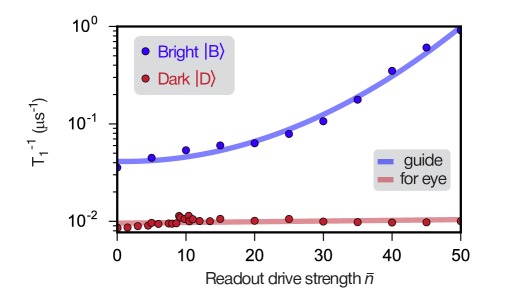
Фигура 5.1: Measurement-induced energy relaxation $T_{1}(\bar{n})$. Energy relaxation rate ($T_{1}^{-1}$) of $\left|\mathrm{B}\right\rangle$ (blue dots) and $\left|\mathrm{D}\right\rangle$ (red dots) as a function of $\bar{n}$, measured with the following protocol: after the atom is prepared in either $\left|\mathrm{B}\right\rangle$ or $\left|\mathrm{D}\right\rangle$, the readout tone ($\mathrm{R}$) is turned on for duration $t_{\mathrm{read}}$ with amplitude $\bar{n}$ (corresponding to the number of steady-state photons in the readout cavity when excited on resonance), whereafter, the population of the initial state is measured. As in all other experiments, the readout drive is applied at the $\left|\mathrm{B}\right\rangle$ cavity frequency ($\omega_{\mathrm{C}}-\chi_{\mathrm{B}}$). The relaxation rates are extracted from exponential fits of the population decay as a function of $t_{\mathrm{read}}$, from $1.3\times 10^{7}$ experimental realizations. The solids lines are guides to the eye: blue line indicates the rapid degradation of $T_{1}^{\mathrm{B}}$ as a function of the readout strength, while the red line indicates the nearly constants $T_{1}^{\mathrm{D}}$ of the protected dark level.

5.2 Control of the three-level atom

5.2.1 Qubit pulses

The implementation of precise and coherent manipulation of the three-level atom is important for the tomographic reconstruction of the flight of the quantum jump as well the ability to faithfully reverse it. One of the main sources of pulse infidelity is typically decoherence, but the rather long coherence time of the Darkmon device relative to the duration of the pulses employed in the experiment make it largely unimportant, and instead, place emphasis on the technical details of pulse generation and Hamiltonian non-idealities, such as leakage to higher excited states.

Mitigation of main technical non-idealities. The effect of the zero-order hold of the FPGA digital-to-analog converter (DAC) was mitigated by installing a 270 MHz low pass filter (Mini-Circuits BLP-300+) on each of the analog output channels, see Sec. 4.5. All microwave tones were generated with single-sideband IQ-controlled modulation at a base intermediate frequency (IF) of 50 MHz, and the lower radio-frequency (RF) sideband was used for the control tones (detuned 50 MHz below the local oscillator (LO) frequency). The IQ mixers were calibrated with a four stage iterative routine to minimize carrier leakage, by tuning the DC offsets of the I and Q channels, and to suppress the RF image, by minimizing the quadrature skew and IQ gain imbalance. The LO leakage could typically be suppressed to $\approx-70$ dB relative to the RF tone. Spurious intermodulation tones generated by higher-order non-linear terms present in the mixers [i.e., third-order intercept-point (IP3) products] were generally negligible as the mixers were not typically driven near saturation, but bandpass filters were installed on the RF outputs of all mixers to nonetheless suppress any spurious tones. Excess noise from the following RF amplifier (MiniCircuits ZVA-183-S+) was suppressed by 80 dB when the control drives were turned off by use of a high-isolation SPST switch (Analog Device HMC-C019).

The pulses applied to the Dark and Bright transition were calibrated with a combination of Rabi, derivative removal via adiabatic gate (DRAG) (Chow et al., 2010), All-XY (Reed, 2013), and amplitude pulse train sequences (Bylander et al., 2011). Pulse timings and delays, especially between the analog channels and the SPST switch digital markers, were calibrated with a wide-bandwidth oscilloscope with ultra-low jitter (Keysight 86100D Infiniium DCA-X). The alignment was verified by performing a Gaussian qubit $\pi$ pulse on the GB transition and varying the delay between the rise of the SPST digital marker and the signal on the analog IQ pair playing the pulse.

5.2.2 Tomography of the three-level atom

At the end of each experimental realization, we performed one of 15 rotation sequences on the atom that transferred information about one component of the density matrix, $\hat{\rho}_{a}$, to the population of $\left|\mathrm{B}\right\rangle$, which was measured with a 600 ns square pulse on the readout cavity. Pulses were calibrated as discussed in Sec. 5.2.1. The readout signal was demodulated with the appropriate digital filter function required to realize temporal mode matching (Eichler et al., 2012). To remove the effect of potential systematic offset errors in the readout signal, we subtracted the measurement results of operator components of $\hat{\rho}_{a}$ and their opposites. From the measurement results of this protocol, we reconstructed the density matrix $\hat{\rho}_{a}$, and subsequently parametrized it the useful form

$$\hat{\rho}_{a}=\begin{pmatrix}\frac{N}{2}\left(1-Z_{\mathrm{GD}}\right)&\frac{N}{2}\left(X_{\mathrm{GD}}+iY_{\mathrm{GD}}\right)&R_{\mathrm{BG}}+iI_{\mathrm{BG}}\\ \frac{N}{2}\left(X_{\mathrm{GD}}-iY_{\mathrm{GD}}\right)&\frac{N}{2}\left(1+Z_{\mathrm{GD}}\right)&R_{\mathrm{BD}}+iI_{\mathrm{BD}}\\ R_{\mathrm{BG}}-iI_{\mathrm{BG}}&R_{\mathrm{BD}}-iI_{\mathrm{BD}}&1-N\end{pmatrix},$$ (5.2)

where $X_{\mathrm{GD}},Y_{\mathrm{GD}},$ and $Z_{\mathrm{GD}}$ are the Bloch vector components of the GD manifold, $N$ is the total population of the $\left|\mathrm{G}\right\rangle$ and $\left|\mathrm{D}\right\rangle$ states, while $R_{\mathrm{BG}},R_{\mathrm{BD}},I_{\mathrm{BG}}$ and $I_{\mathrm{BD}}$ are the coherences associated with $\left|\mathrm{B}\right\rangle$, relative to the GD manifold. The measured population in $\left|\mathrm{B}\right\rangle$, $1-N$, remains below 0.03 during the quantum jump, see Fig. 5.3. Tomographic reconstruction was calibrated and verified by preparing Clifford states, accounting for the readout fidelity of 97%.

Control experiment.

In Fig. 5.2, we show the results of a control experiment where we verified the Ramsey coherence ($T_{\mathrm{2R}}^{\mathrm{D}}$) and energy relaxation ($T_{\mathrm{1}}^{\mathrm{D}}$) times of the DG transition with our tomography method. Solid lines are fitted theoretical curves for the free evolution of the prepared initial state $\frac{1}{\sqrt{2}}\left(\left|\mathrm{D}\right\rangle-\left|\mathrm{G}\right\rangle\right)$. The $T_{\mathrm{2R}}^{\mathrm{D}}=119.2\,\mathrm{\mu s}$ value gained from the simultaneous fit of $X_{\mathrm{DG}}(t)$ and $Y_{\mathrm{DG}}(t)$ matches the lifetime independently obtained from a standard $T_{\mathrm{2R}}$ measurement. Similarly, the value of $T_{\mathrm{1}}^{\mathrm{D}}=115.4\,\mathrm{\mu s}$ extracted from an exponential fit of $Z_{\mathrm{DG}}(t)$ matches the value obtained from a standard $T_{\mathrm{1}}$ measurement. We note that our tomography procedure is well calibrated and skew-free, as evident in the zero steady-state values of $X_{\mathrm{DG}}$ and $Y_{\mathrm{DG}}$. The steady state $Z_{\mathrm{DG}}$ corresponds to the thermal population of the dark state $n_{\mathrm{th}}^{\mathrm{D}}$. It has recently been shown that residual thermal populations in cQED systems can be significantly reduced by properly thermalizing the input-output lines (Yeh et al., 2017, Wang et al., 2019).

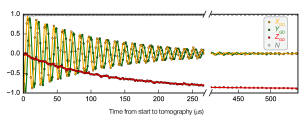
Фигура 5.2: Control experiment: time-resolved tomogram of the free evolution of a DG superposition. The atom is prepared in $\frac{1}{\sqrt{2}}\left(\left|\mathrm{D}\right\rangle-\left|\mathrm{G}\right\rangle\right)$ and tomography is performed after a varied delay. Dots: reconstructed conditional GD tomogram ($X_{\mathrm{DG}},Y_{\mathrm{DG}}$, and $Z_{\mathrm{DG}}$) and population in DG manifold, $N$, see Eq. (5.2). Solid lines: theoretical fits.

Mid-flight tomogram.

In the presence of the coherent Rabi drive $\Omega_{\mathrm{DG}}$ (corresponding to catch parameter $\Delta t_{\mathrm{off}}=0$), the complete tomogram of the three-level atom was reconstructed, and a slice at the mid-flight time, $\Delta t_{\mathrm{mid}}$, is shown in Fig. 5.3. All imaginary components of the reconstructed conditional density matrix, $\rho_{\mathrm{c}}$, are negligibly small, less than 0.007, as expected, see Sec. 5.5, for well-calibrated tomographic phase control. The population of the $\left|\mathrm{B}\right\rangle$ state, 0.023, is nearly negligible as well, as it is conditioned away by the IQ filter, see Sec. 5.3.1.

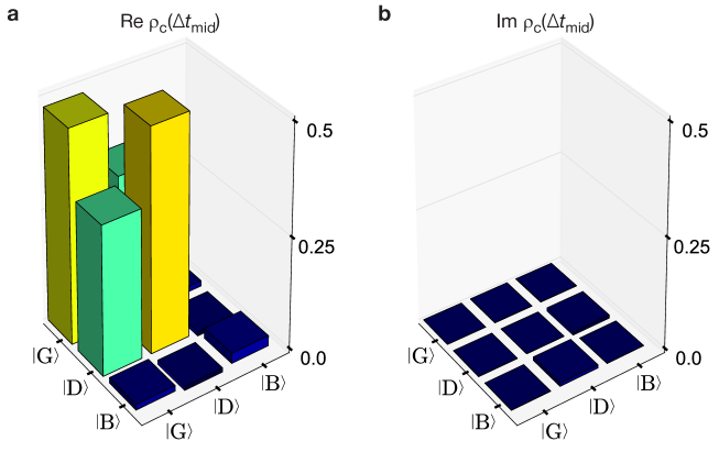
Фигура 5.3: Mid-flight tomogram. The plots show the real (a) and imaginary (b) parts of the conditional density matrix, $\rho_{\mathrm{c}}$, at the mid flight of the quantum jump ($\Delta t_{\mathrm{catch}}=\Delta t_{\mathrm{mid}}$), in the presence of the Rabi drive from $\left|\mathrm{G}\right\rangle$ to $\left|\mathrm{D}\right\rangle$ ($\Delta t_{\mathrm{off}}=0$). The population of the $\left|\mathrm{B}\right\rangle$ state is 0.023, and the magnitude of all imaginary components is less than 0.007.

5.2.3 Atom and cavity drives

In all experiments, unless noted otherwise, the following drive parameters were used: The DG Rabi drive, $\Omega_{\mathrm{DG}}$, was applied 275 kHz below $\omega_{\mathrm{D}}$ to account for the Stark shift of the cavity. The BG drive, $\Omega_{\mathrm{BG}}$, was realized as a bi-chromatic tone in order to unselectively address the BG transition, which was broadened and Stark shifted due to the coupling between $\left|\mathrm{B}\right\rangle$ and the readout cavity. Specifically, we addressed transitions from $\left|\mathrm{G}\right\rangle$ to $\left|\mathrm{B}\right\rangle$ with a Rabi drive $\Omega_{\mathrm{B0}}/2\pi=1.20\pm 0.01\,$ MHz at frequency $\omega_{\mathrm{BG}}$, whereas transitions from $\left|\mathrm{B}\right\rangle$ to $\left|\mathrm{G}\right\rangle$ were addressed with a Rabi drive $\Omega_{\mathrm{B1}}/2\pi=0.60\pm 0.01\,$ MHz tuned 30 MHz below $\omega_{\mathrm{BG}}$. This bi-chromatic scheme provided the ability to tune the up-click and down-click rates independently, but otherwise essentially functioned as an incoherent broad-band source. In Table 5.2, we summarize the hierarchy of timescales established by the drive amplitudes and frequencies as well as the relevant decoherence properties of the atom.

Symbol	Value	Description
$\Gamma^{-1}$	$\approx 8.8$ ns	Effective measurement time of $\left|\mathrm{B}\right\rangle$, approximately given by $1/\kappa\bar{n}$, where $\bar{n}=5\pm 0.2$ in the main experiment
$\kappa^{-1}$	$44.0\pm 0.06$ ns	Readout cavity lifetime
$T_{\mathrm{int}}$	260.0 ns	Integration time of the measurement record, set in the controller at the beginning of the experiment
$\Gamma_{\mathrm{BG}}^{-1}$	$0.99\pm 0.06\,\mathrm{\mu s}$	Average time the atom rests in $\left|\mathrm{G}\right\rangle$ before an excitation to $\left|\mathrm{B}\right\rangle$, see Fig. 1.2b
$\Delta t_{\mathrm{mid}}$	$3.95\,\mathrm{\mu s}$	No-click duration for reaching $Z_{\mathrm{GD}}=0$ in the flight of the quantum jump from $\left|\mathrm{G}\right\rangle$ to $\left|\mathrm{D}\right\rangle$, in the full presence of $\Omega_{\mathrm{DG}}$, see Fig. 1.3b
$\Gamma_{\mathrm{GD}}^{-1}$	$30.8\pm 0.4\,\mathrm{\mu s}$	Average time the atom stays in $\left|\mathrm{D}\right\rangle$ before returning to $\left|\mathrm{G}\right\rangle$ and being detected, see Fig. 1.2b
$T_{1}^{\mathrm{D}}$	$116\pm 5\,\mathrm{\mu s}$	Energy relaxation time of $\left|\mathrm{D}\right\rangle$
$T_{2\mathrm{R}}^{\mathrm{D}}$	$120\pm 5\,\mathrm{\mu s}$	Ramsey coherence time of $\left|\mathrm{D}\right\rangle$
$T_{2\mathrm{E}}^{\mathrm{D}}$	$162\pm 6\,\mathrm{\mu s}$	Echo coherence time of $\left|\mathrm{D}\right\rangle$
$\Gamma_{\mathrm{DG}}^{-1}$	$220\pm 5\,\mathrm{\mu s}$	Average time between two consecutive $\left|\mathrm{G}\right\rangle$ to $\left|\mathrm{D}\right\rangle$ jumps

Таблица 5.2: Summary of timescales. List of the characteristic timescales involved in the catch and reverse experiment. The Hamiltonian parameters of the system are summarized in Sec. 5.1.

5.3 Monitoring quantum jumps in real time

5.3.1 IQ filter

To mitigate the effects of imperfections in the atom readout scheme in extracting a $\left|\mathrm{B}\right\rangle$/not-$\left|\mathrm{B}\right\rangle$ result, we applied a two-point, hysteretic IQ filter, implemented on the FPGA controller in real time. The filter is realized by comparing the present quadrature record values $\left\{I_{\mathrm{rec}},Q_{\mathrm{rec}}\right\}$, with three thresholds ($I_{\mathrm{B}},I_{\bar{\mathrm{B}}},$ and $Q_{\mathrm{B}}$) in the following way:

Input:	$Q_{\mathrm{rec}}\geq Q_{\mathrm{B}}$ or $I_{\mathrm{rec}}>I_{\mathrm{B}}$	$Q_{\mathrm{rec}}<Q_{\mathrm{B}}$ and $I_{\mathrm{rec}}<I_{\bar{\mathrm{B}}}$	$Q_{\mathrm{rec}}<Q_{\mathrm{B}}$ and $I_{\bar{\mathrm{B}}}\leq I_{\mathrm{rec}}\leq I_{\mathrm{B}}$
Output:	$\left|\mathrm{B}\right\rangle$	not-$\left|\mathrm{B}\right\rangle$	previous

The filter and thresholds were selected to provide a best estimate of the time of a click, operationally understood as a change in the filter output from $\left|\mathrm{B}\right\rangle$ to not-$\left|\mathrm{B}\right\rangle$. The $I_{{\mathrm{B}}}$ and $I_{\bar{\mathrm{B}}}$ thresholds were chosen 1.5 standard deviations away from the I-quadrature mean of the $\left|\mathrm{B}\right\rangle$ and not-$\left|\mathrm{B}\right\rangle$ distributions, respectively. The $Q_{{\mathrm{B}}}$ threshold was chosen 3 standard deviations away from the Q-quadrature mean. Higher excited states of the atom were selected out by $Q_{\mathrm{rec}}$ values exceeding the $Q_{\mathrm{B}}$ threshold.

5.3.2 Unconditioned monitoring

In Sec. 1.2, we described a protocol for the unconditioned monitoring of the quantum jumps where the atom is subject to the continuous Rabi drives $\Omega_{\mathrm{BG}}$ and $\Omega_{\mathrm{DG}}$, as depicted in Fig. 1.1. From the continuous tracking of the quantum jumps, over 3.2 s. of data, we histogrammed the times, $\tau_{\operatorname{not-B}}$, spent in not-$\left|\mathrm{B}\right\rangle$, Fig. 1.2b. In Fig. 5.4, we show the complimentary histogram for the times, $\tau_{{\rm B}},$ spent in $\left|\mathrm{B}\right\rangle$, which is unlike the latter, in that it follows a single exponential decay law. This single Poisson process character follows from the fact that the $\left|\mathrm{B}\right\rangle$ measurement result collapses the atom to a single state, $\left|\mathrm{B}\right\rangle$, unlike the not-$\left|\mathrm{B}\right\rangle$ result. The average time spent in $\left|\mathrm{B}\right\rangle$, extracted from the fit, is $\bar{\tau}_{{\rm B}}=4.2\pm 0.03\,\mathrm{\mu s}$.

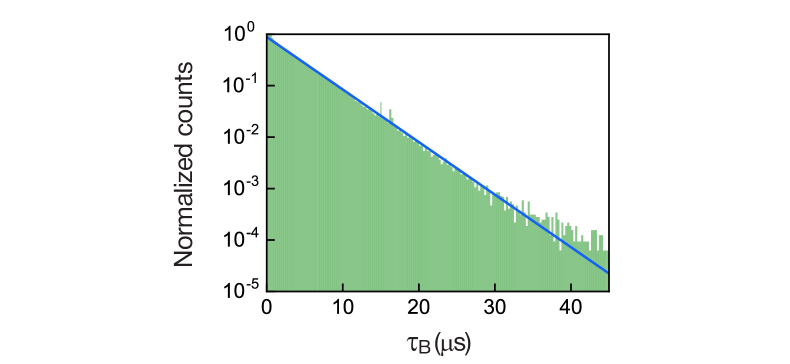
Фигура 5.4: Waiting time to switch from a $\left|\mathrm{B}\right\rangle$ to not-$\left|\mathrm{B}\right\rangle$ state assignment result. Semi-log plot of the histogram (shaded green) of the duration of times corresponding to $\left|\mathrm{B}\right\rangle$-measurement results, $\tau_{\operatorname{B}}$, for 3.2 s of continuous data of the type shown in Fig. 1.2a. Solid line is an exponential fit, which yields a $4.2\pm 0.03\,\mathrm{\mu s}$ time constant.

5.4 Catching and reversing the jump

5.4.1 Experiment flow

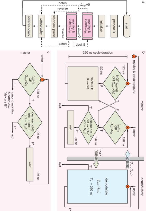
Фигура 5.5: Experiment flow. See text for detailed description.

Figure 5.5a shows a flowchart representation of steps involved in the catch and reverse protocol. In the following, we describe each block in the diagram in the order in which it would be executed.

Start:

internal memory registers are set to zero (Ofek et al., 2016, Liu, 2016), including the no-click counter ‘‘cnt,’’ defined below.

Prepare B:

controller deterministically prepares the atom in $\left|\mathrm{B}\right\rangle$, a maximally conservative initial state, with measurement-based feedback (Ristè et al., 2012a).

Initialize:

controller turns on the atom ($\Omega_{\mathrm{BG}}$ and $\Omega_{\mathrm{DG}}$) and cavity drives ($\mathrm{R}$) and begins demodulation.

Monitor and catch $\Delta t_{\mathrm{on}}$:

with all drives on ($\Omega_{\mathrm{BG}},\Omega_{\mathrm{DG}}$, and $\mathrm{R}$), the controller actively monitors the cavity output signal until it detects no-clicks for duration $\Delta t_{\mathrm{on}}$, as described in panel (b), whereafter, the controller proceeds to ‘‘monitor and catch $\Delta t_{\mathrm{off}}$’’ in the case that $\Delta t_{\mathrm{off}}>0$; otherwise, for $\Delta t_{\mathrm{off}}=0$, the controller proceeds to ‘‘tomography’’ (‘‘feedback pulse’’) for the catch (reverse) protocol.

Monitor and catch $\Delta t_{\mathrm{off}}$:

with the Rabi drive $\Omega_{\mathrm{DG}}$ off, while keeping the drives $\Omega_{\mathrm{BG}}$ and R on, the controller continues to monitor the output signal. The controller exits the routine only if it detects a click, proceeding to the ‘‘declare B’’ step of the ‘‘monitor and catch $\Delta t_{\mathrm{on}}$’’ routine, or if no further clicks are detected for the pre-defined duration $\Delta t_{\mathrm{off}}$, proceeding to ‘‘tomography’’ (‘‘feedback pulse’’) for the catch (reverse) protocol.

Feedback pulse:

with all the continuous drives turned off, the controller performs a pulse on the DG transition of the atom, defined by the two angles $\left\{\theta_{I}\left(\Delta t_{\mathrm{catch}}\right),\varphi_{I}\left(\Delta t_{\mathrm{catch}}\right)\right\}$.

Tomography:

controller performs next-in-order tomography sequence (see Sec. 5.2.2) while the demodulator finishes processing the final data in its pipeline.

Advance tomo.:

tomography sequence counter is incremented, and after a $50\leavevmode\nobreak\ \mathrm{\mu s}$ delay, the next realization of the experiment is started.

Logic and timing of catch subroutines

Monitor and catch $\Delta t_{\mathrm{on}}$.

Figure 5.5b shows a concurrent-programming flowchart representation of the ‘‘monitor and catch $\Delta t_{\mathrm{on}}$’’ routine. Displayed are the master and demodulator modules of the controller. The demodulator outputs a pair of 16 bit signed integers, $\left\{I_{\mathrm{rec}},Q_{\mathrm{rec}}\right\}$, every $T_{\mathrm{int}}=260$ ns, which is routed to the master module, as depicted by the large left-pointing arrow. The master module implements the IQ filter (see Sec. 5.3.1) and tracks the number of consecutive not-$\left|\mathrm{B}\right\rangle$ measurement results with the counter cnt. The counter thus keeps track of the no-click time elapsed since the last click, which is understood as a change in the measurement result from $\left|\mathrm{B}\right\rangle$ to not-$\left|\mathrm{B}\right\rangle$. When the counter reaches the critical value $N_{\mathrm{on}}$, corresponding to $\Delta t_{\mathrm{on}}$, the master and demodulator modules synchronously exit the current routine, see the T* branch of the ‘‘declare not-B’’ decision block. Until this condition is fulfilled (F*), the two modules proceed within the current routine as depicted by the black flowlines.

To minimize latency and maximize computation throughput, the master and demodulator were designed to be independent sequential processes running concurrently on the FPGA controller, communicating strictly through synchronous message passing, which imposed stringent synchronization and execution time constraints. All master inter-module logic was constrained to run at a 260 ns cycle, the start of which necessarily was imposed to coincide with a ‘‘receive & stream record’’ operation, here, denoted by the stopwatch. In other words, this imposed the algorithmic constraint that all flowchart paths staring at a stopwatch and ending in a stopwatch, itself or other, were constrained to a 260 ns execution timing. A second key timing constraint was imposed by the time required to propagate signals between the different FPGA cards, which corresponded to a minimum branching-instruction duration of 76 ns.

Monitor and catch $\Delta t_{\mathrm{off}}$.

Figure 5.5c shows a concurrent-programming flowchart representation of the master module of the ‘‘monitor and catch $\Delta t_{\mathrm{off}}$’’ routine. The corresponding demodulation-module flowchart is identical to that shown of panel (b); hence, it is not shown. This routine functions in following manner: If a $\left|\mathrm{B}\right\rangle$ outcome is detected, the controller jumps to the ‘‘declare B’’ block of the monitor & catch $\Delta t_{\mathrm{on}}$ routine; otherwise, when only not-$\left|\mathrm{B}\right\rangle$ outcomes are observed, and the counter reaches the critical value $N_{\mathrm{off}}$, corresponding to $\Delta t_{\mathrm{catch}}=\Delta t_{\mathrm{on}}+\Delta t_{\mathrm{off}}$, the controller exits the routine.

5.5 Comparison between theory and experiment

In this section, we present the comparison between the results of the quantum jumps experiment and the predictions of the quantum trajectory theory of the experiment developed in Chapter 3. The results agree with the theoretical predictions, accounting for known imperfections, essentially without adjustable parameters. Simulation plots courtesy of H.J. Carmichael.

5.5.1 Simulated data sets

Independently measured parameters.

The parameters used in the Monte Carlo simulation described in Sec. 3.2.2 are listed in Table 5.3. Nearly all are set to the value at the center of the range quoted in Table 5.1, with three exceptions: i) $T_{1}^{{\rm B}}$ and $T_{1}^{{\rm D}}$ are set to lower values in response to the photon number dependence of the readout displayed in Fig. 5.1, ii) $\Omega_{{\rm DG}}/2\pi$ is set higher, but still falls inside the experimental error bars, and iii) $n_{{\rm th}}^{{\rm C}}=0$. Notably, of the three exceptions, only $\Omega_{{\rm DG}}/2\pi$ has a noticeable effect on the comparison between simulated and experimental data sets.

Leakage from the GBD-manifold.

As discussed in Sec. 4.1, see Fig. 4.2, the Darkmon system has higher excited states, which are generally unimportant, but do contribute a small imperfection that needs to be considered to qualitatively account for the results. As discussed in Sec. 3.2.2, we model the effect of leakage from the GBD manifold by adding a single additional higher-excited state level, denoted $\left|\mathrm{F}\right\rangle.$ The additional random jumps to state $|{\rm F}\rangle$ are governed by four parameters that are not independently measured; they serve as fitting parameters, required to bring the simulation into agreement with the asymptotic behavior of ${\rm Z}(\Delta t_{{\rm catch}})$, which, without leakage to $|{\rm F}\rangle$, settles to a value higher than is measured in the experiment. The evolution of the ${\rm X}(\Delta t_{{\rm catch}})$ is largely unaffected by the assignment of these parameters, where any change that does occur can be offset by adjusting $\Omega_{{\rm DG}}/2\pi$ while staying within the experimental error bars.

Ensemble average.

Simulated data sets are computed as an ensemble average by sampling an ongoing Monte Carlo simulation, numerically implementing the model outlined in Eqs. (3.58)–(3.65). Quadratures $I_{{\rm rec}}$ and $Q_{{\rm rec}}$ are computed from Eqs. (3.56) and (3.57), digitized with integration time $T_{{\rm int}}=260\mkern 2.0mu{\rm ns}$, and then, as in the experiment, a hysteric filter is used to locate ‘‘click’’ events ($\Delta t_{{\rm catch}}=0$) corresponding to an inferred change of state from $|{\rm B}\rangle$ to not-$|{\rm B}\rangle$. During the subsequent sampling interval ($\Delta t_{{\rm catch}}\geq 0$), the four quantities

$$\big{(}{\rm Z}_{{\rm GD}}^{j},{\rm X}_{{\rm GD}}^{j},{\rm Y}_{{\rm GD}}^{j},{\rm P}_{{\rm BB}}^{j}\big{)}(\Delta t_{{\rm catch}})=\big{(}{\rm Z}_{{\rm GD}}^{{\rm rec}},{\rm X}_{{\rm GD}}^{{\rm rec}},{\rm Y}_{{\rm GD}}^{{\rm rec}},{\rm P}_{{\rm BB}}^{{\rm rec}}\big{)}(t_{j}+\Delta t_{{\rm catch}}),$$ (5.3)

with $t_{j}$ is the click time and

$${\rm Z}_{{\rm GD}}^{{\rm rec}}(t) = \frac{\langle{\rm D}|\psi(t)\rangle\langle\psi(t)|{\rm D}\rangle-\langle{\rm G}|\psi(t)\rangle\langle\psi(t)|{\rm G}\rangle}{\langle\psi(t)|\psi(t)\rangle},$$ (5.4)

$${\rm X}_{{\rm GD}}^{{\rm rec}}(t)+i{\rm Y}_{{\rm GD}}^{{\rm rec}}(t) = 2\frac{\langle{\rm D}|\psi(t)\rangle\langle\psi(t)|{\rm G}\rangle}{\langle\psi(t)|\psi(t)\rangle},$$ (5.5)

$${\rm P}_{{\rm BB}}^{{\rm rec}}(t) = \frac{\langle{\rm B}|\psi(t)\rangle\langle\psi(t)|{\rm B}\rangle}{\langle\psi(t)|\psi(t)\rangle},$$ (5.6)

are computed, and running sums of each are updated. The sample terminates when the measurement record indicates a change of state from not-$|{\rm B}\rangle$ back to $|{\rm B}\rangle$. Finally, for comparison with the experiment, Bloch vector components are recovered from the average over sample intervals via the formula

$$\big{(}{\rm Z}_{{\rm GD}},{\rm X}_{{\rm GD}},{\rm Y}_{{\rm GD}}\big{)}(\Delta t_{{\rm catch}})=\frac{\sum_{j}^{N(\Delta t_{{\rm catch}})}\big{(}{\rm Z}_{{\rm GD}}^{j},{\rm X}_{{\rm GD}}^{j},{\rm Y}_{{\rm GD}}^{j}\big{)}(\Delta t_{{\rm catch}})}{N(\Delta t_{{\rm catch}})-\sum_{j}^{N(\Delta t_{{\rm catch}})}P_{{\rm BB}}^{j}(\Delta t_{{\rm catch}})},$$ (5.7)

where $N(\Delta t_{{\rm catch}})$ is the number of sample intervals that extend up to, or beyond, the time $\Delta t_{{\rm catch}}$. The simulation and sampling procedure is illustrated in Fig. 5.6, and a comparison between the experiment and the simulation is provided in Fig. 5.7.

The simulated and measured Bloch vector components are fit with expressions motivated by Eqs. (3.18)-(3.20) and (3.44), modified to account for the effect of non-idealities in the experiment,

$$\mathrm{Z}_{\text{GD}}(\Delta t_{\operatorname{catch}}) =a+b\tanh(\Delta t_{\operatorname{catch}}/\tau+c),$$ (5.8)

$$\mathrm{X}_{\text{GD}}(\Delta t_{\operatorname{catch}}) =a^{\prime}+b^{\prime}\operatorname{sech}(\Delta t_{\operatorname{catch}}/\tau^{\prime}+c^{\prime})\,,$$ (5.9)

$$\mathrm{Y}_{\text{GD}}(\Delta t_{\operatorname{catch}}) =0\,.$$ (5.10)

The fit parameters ($a,a^{\prime},b,b^{\prime},c,c^{\prime},\tau,\tau^{\prime}$) for the simulated and experimental data shown in Fig. 5.7 are compared in Table 5.4. As imposed by Eq. (3.44), in the absence of $\Omega_{{\rm DG}}$ (turned off at time $\Delta t_{{\rm on}}=2\mkern 2.0mu\mu{\rm s}$) $a^{\prime}$, the offset of $\mathrm{X}_{\text{GD}}$, is strictly enforced to be zero. The extracted simulation and experiment parameters are found to agree at the percent level.

Readout cavity		BG transition		DG transition
Non-linear parameters
		$\chi_{\mathrm{B}}/2\pi=$	$-5.08\,\mathrm{MHz}$	$\chi_{\mathrm{D}}/2\pi=$	$-0.33\,\mathrm{MHz}$
Coherence related parameters
$\kappa/2\pi$=	$3.62\mathrm{MHz}$	$T_{\mathrm{1}}^{\mathrm{B}}=$	$15\,\mathrm{\mu s}$	$T_{\mathrm{1}}^{\mathrm{D}}=$	$105\,\mathrm{\mu s}$
$\eta=$	$0.33$	$T_{\mathrm{2\mathrm{R}}}^{\mathrm{B}}=$	$18\,\mathrm{\mu s}$	$T_{\mathrm{2\mathrm{R}}}^{\mathrm{D}}=$	$120\,\mathrm{\mu s}$
$T_{\mathrm{int}}=$	$260.0\,\mathrm{ns}$
$n_{\mathrm{th}}^{\mathrm{C}}=$	$0$	$n_{\mathrm{th}}^{\mathrm{B}}=$	$0.01$	$n_{\mathrm{th}}^{\mathrm{D}}=$	$0.05$
Drive amplitude and detuning parameters
$\bar{n}=$	$5.0$	$\Omega_{\mathrm{B}0}/2\pi=$	$1.20\,\mathrm{MHz}$	$\Omega_{\mathrm{DG}}/2\pi=$	$21.6\,\mathrm{kHz}$
		$\Omega_{\mathrm{B}1}/2\pi=$	$0.60\,\mathrm{MHz}$
$\Delta_{\mathrm{R}}=$	$\chi_{\mathrm{B}}$	$\Delta_{\mathrm{B}1}/2\pi=$	$-30.0\,\text{MHz}$	$\Delta_{\mathrm{DG}}/2\pi=$	$-274.5\,\text{kHz}$

Таблица 5.3: Compilation of the simulation parameters.

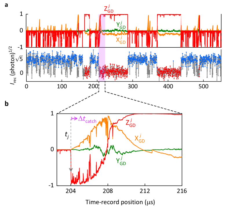
Фигура 5.6: Sampling of the Monte-Carlo simulation. a, Simulated measurement quadrature $I_{{\rm rec}}$ and correlated trajectory computed from Eqs. (5.4) and (5.5). Three sample intervals are shown. The earliest corresponds to leakage from the GBD-manifold, where a jump from $|{\rm G}\rangle$ to $|{\rm F}\rangle$ is followed by a jump from $|{\rm F}\rangle$ to $|{\rm D}\rangle$. The second and third sample intervals correspond to direct transitions from $|{\rm G}\rangle$ to $|{\rm D}\rangle$, which are continuously monitored and the object of the experiment. b, Expanded view of the shaded region of the second sample interval in panel (a). The evolution is continuous but not smooth, due to backaction noise from the continuously monitored readout. This feature is in sharp contrast to the perfect ‘‘no-click’’ readout upon which the simple theory of Sec. 3.1 is based. Figure courtesy of H.J. Carmichael.

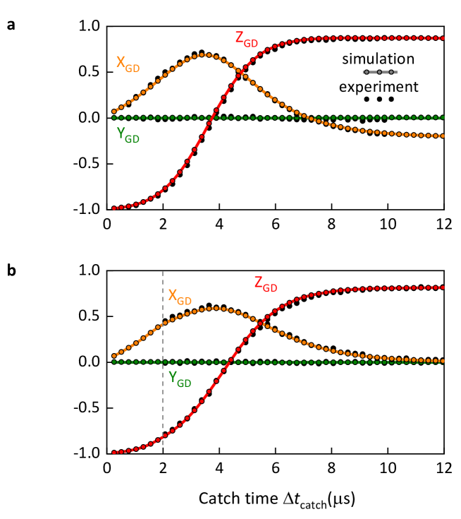
Фигура 5.7: Comparison between simulation and experiment. a, Simulated data set obtained with Rabi drive $\Omega_{{\rm DG}}$ turned on for the entire $\Delta t_{{\rm catch}}$; parameters taken from Table 5.3 and leakage from the GBD-manifold included with $(\gamma_{{\rm FG}},\gamma_{{\rm FD}})/2\pi=0.38\mkern 2.0mu{\rm kHz}$ and $(\gamma_{{\rm GF}},\gamma_{{\rm DF}})/2\pi=11.24\mkern 2.0mu{\rm kHz}$. b, Simulated data set obtained with Rabi drive $\Omega_{{\rm DG}}$ turned off at time $\Delta t_{{\rm on}}=2\mkern 2.0mu\mu{\rm s}$; parameters taken from Table 5.3 and leakage from the GBD-manifold included with $\gamma_{{\rm FG}}/2\pi=0.217\mkern 2.0mu{\rm kHz}$, $\gamma_{{\rm FD}}/2\pi=4.34\mkern 2.0mu{\rm kHz}$, $\gamma_{{\rm GF}}/2\pi=11.08\mkern 2.0mu{\rm kHz}$, and $\gamma_{{\rm DF}}/2\pi=15.88\mkern 2.0mu{\rm kHz}$. When leakage from the GBD-manifold is omitted, the ${\rm Z}_{{\rm GD}}$ curve rises more sharply and settles to a value that is 10% (20%) higher in panel (a) (panel (b)). Figure courtesy of H.J. Carmichael.

(a) In presence of $\Omega_{\mathrm{DG}}$

Parameter Experiment Simulation Error $a$ -0.07 $\pm$ 0.005 -0.07 $\pm$ 0.005 0.5% $a^{\prime}$ -0.21 $\pm$ 0.005 -0.22 $\pm$ 0.005 2% $b$ 0.94 $\pm$ 0.005 0.95 $\pm$ 0.005 1% $b^{\prime}$ 0.93 $\pm$ 0.005 0.91 $\pm$ 0.005 2% $c$ -2.32 $\pm$ 0.03 -2.27 $\pm$ 0.03 2% $c^{\prime}$ -2.04 $\pm$ 0.03 -2.05 $\pm$ 0.03 0.5% $\tau$ 1.64 $\pm$ 0.01 1.65 $\pm$ 0.01 0.5% $\tau^{\prime}$ 1.74 $\pm$ 0.01 1.76 $\pm$ 0.01 1%

(b) In absence of $\Omega_{\mathrm{DG}}$

Parameter Experiment Simulation Error $a$ -0.11 $\pm$ 0.005 -0.10 $\pm$ 0.005 8% $a^{\prime}$ 0 $\pm$ 0 0 $\pm$ 0 0% $b$ 0.92 $\pm$ 0.008 0.91 $\pm$ 0.008 1% $b^{\prime}$ 0.61 $\pm$ 0.005 0.60 $\pm$ 0.005 2% $c$ -1.96 $\pm$ 0.05 -2.10 $\pm$ 0.05 7% $c^{\prime}$ -1.97 $\pm$ 0.05 -2.05 $\pm$ 0.05 4% $\tau$ 2.17 $\pm$ 0.05 2.03 $\pm$ 0.05 6% $\tau^{\prime}$ 1.98 $\pm$ 0.05 1.92 $\pm$ 0.05 3%

Таблица 5.4: Comparison between parameters extracted from the simulation and those from the experiment. a, Parameters obtained from fits of the simulated and measured data for the catch protocol in the presence of the Rabi drive $\Omega_{{\rm DG}}$ throughout the entire duration of the quantum jump, data shown in Fig. 5.7a. b, Parameters obtained from fits of the simulated and measured data for the catch protocol in the absence of the $\Omega_{{\rm DG}}$ during the flight of the quantum jump for $\Delta t_{\mathrm{on}}=2\mathrm{\ \mu s}$, data shown in Fig. 5.7b.

5.5.2 Error budget

In this section, we examine the effect of the various imperfections and dissipation channels on the fidelity of the catch protocol.

Imperfections.

The various imperfections are expected to reduce the maximum coherence recovered in the measurement of ${\rm X}_{{\rm GD}}(\Delta t_{{\rm catch}})$. They include:

1. Readout errors when inferring $|{\rm B}\rangle$ to not-$|{\rm B}\rangle$ transitions and the reverse. Such errors affect the assignment of $\Delta t_{{\rm catch}}$, which can be either too short or too long to correlate correctly with the true state of the system.

2. Leaks from the GBD-manifold to higher excited states. Importantly, these errors mimic a $|{\rm B}\rangle$ to not-$|{\rm B}\rangle$ transition, as in the first sample interval of Fig. 5.6, but the anticipated coherent evolution within the GBD-manifold does not occur. In this manner, the excitations to higher states lead to false detections.

3. Thermal jumps from $|{\rm G}\rangle$ to $|{\rm D}\rangle$. Such incoherent transitions contribute in a similar way to ${\rm Z}_{{\rm GD}}(\Delta t_{{\rm catch}})$, while making no contribution to the measured coherence.

4. Direct dephasing of the DG-coherence, $T_{\mathrm{2R}}^{\mathrm{D}}$.

5. Partial distinguishability of $|{\rm G}\rangle$ and $|{\rm D}\rangle$. The readout cavity is not entirely empty of photons when the state is not-$|{\rm B}\rangle$, in which case the cross-Kerr interaction $\chi_{{\rm D}}|{\rm D}\rangle\langle{\rm D}|\hat{c}^{\dagger}\hat{c}$ shifts the $\Omega_{{\rm DG}}$ Rabi drive from resonance; hence, backaction noise is transferred from the photon number to ${\rm X_{{\rm GD}}}(\Delta t_{{\rm catch}})$.

Budget for lost coherence.

The maximum coherence reported in the experiment is $0.71\pm 0.005$. In the simulation it is a little lower at 0.69. By removing the imperfections from the simulation, one by one, we can assign a fraction of the total coherence loss to each. Readout errors are eliminated by identifying transitions between $|{\rm B}\rangle$ and not-$|{\rm B}\rangle$ in the ket $|\psi\rangle$ rather than from the simulated measurement record; all other imperfections are turned off by setting some parameter to zero. The largest coherence loss comes from readout errors, whose elimination raises the ${\rm X}_{{\rm GD}}(\Delta t_{{\rm catch}})$ maximum by 0.09. The next largest comes from leakage to higher excited states, which raises the maximum by a further 0.06. Setting $\chi_{{\rm D}}$ to zero adds a further 0.04, and thermal transitions and pure dephasing together add 0.02. Figure 5.8 illustrates the change in the distribution of ${\rm X}_{{\rm GD}}^{j}(\Delta t_{{\rm catch}})$ samples underlying the recovery of coherence. The removal of the finger pointing to the left in panel (a) is mainly brought about by the elimination of readout errors, while the reduced line of zero coherence marks the elimination of leakage to higher excited states. Aside from these two largest changes, there is also a sharpening of the distribution, at a given $\Delta t_{{\rm catch}}$, when moving from panel (a) to panel (b). Having addressed the five listed imperfections, a further 10% loss remains unaccounted for, i.e., the distribution of panel (b) is not a line passing through ${\rm X}_{{\rm GD}}^{j}(\Delta t_{{\rm mid}})=1$. The final 10% is explained by the heterodyne detection backaction noise, a function of the drive and measurement parameters, displayed in panel (b) of Fig. 5.6.

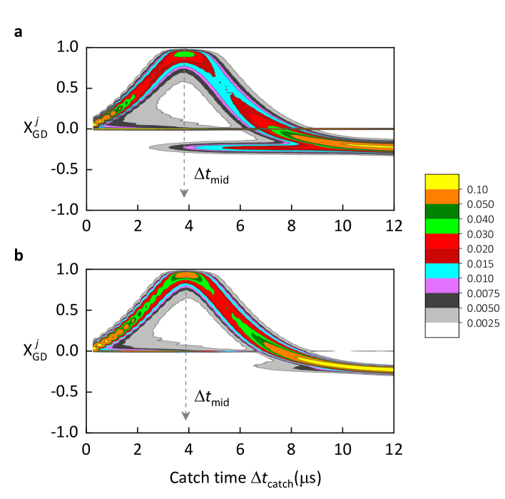
Фигура 5.8: Coherence loss through sample to sample fluctuations. a, Contour plot of the distribution of ${\rm X}_{{\rm GD}}^{j}(\Delta t_{{\rm catch}})$ samples corresponding to the simulated data set displayed in panel (a) of Fig. 5.7. b, Same as panel (a) but with transitions between $|{\rm B}\rangle$ and not-$|{\rm B}\rangle$ identified in the ket $|\psi\rangle$ rather than from the simulated measurement record, and with changed parameters: $(\gamma_{{\rm FG}},\gamma_{{\rm FD}},\gamma_{{\rm GF}},\gamma_{{\rm DF}})/2\pi=0$, $n_{{\rm th}}^{{\rm B}}=n_{{\rm th}}^{{\rm D}}=0$, $T_{2}^{{\rm D}}=2T_{1}^{{\rm D}}$, and $\chi_{{\rm D}}/2\pi=0$. Figure courtesy of H.J. Carmichael.

5.6 Signal-to-noise ratio (SNR) and de-excitation measurement efficiency

The catch protocol hinges on the efficient detection of de-excitations from $|{\rm B}\rangle$ to $|{\rm G}\rangle$, as discussed in more detail in Chapter 3. In atomic physics, de-excitations are typically monitored by a direct detection method, employing a photodetector. Alternatively, de-excitations can be monitored by an indirect method, as done in our experiment. In this section, we discuss the efficiency of both methods. For the indirect method, using simple analytics, we estimate the total efficiency of time-continuous, uninterrupted monitoring of de-excitations from $|{\rm B}\rangle$ to $|{\rm G}\rangle$ to be $\eta_{\mathrm{eff,clk}}=0.90\pm 0.01$ for the parameters of our experiment, with integration time $T_{\mathrm{int}}=0.26\,\mathrm{\mu s}$. The simple analysis of this section complements the numerical one of the previous section, Sec. 5.5.2.

Direct monitoring method in atomic physics. The direct method monitors for a $|{\rm B}\rangle$ de-excitation by collecting and absorbing the photon radiated in the de-excitation. The total measurement efficiency of this method is limited by i) collection efficiency — the fraction of emitted photons collected by the detector in its own input spatial modes (for instance, as determined by the solid angle) — typically falls in the range 0.1 - 50%, (Volz et al., 2011) ii) the efficiency of detecting the absorption of a single photon, which falls in the range 1 - 90%, (Eisaman et al., 2011) and iii) non-idealities of the photodetector apparatus, including its dead time, dark counts, jitter, etc. (Eisaman et al., 2011) The combination of these inefficiencies presents an almost insurmountable challenge in experimental atomic physics for realizing continuous, time-resolved detection of nearly every single photon emitted by the three-level atom, required to faithfully catch the jump.

Direct monitoring method with superconducting circuits. While technologically very different, the direct monitoring method with superconducting circuits is conceptually similar to atomic method but can readily achieve high collection efficiencies (Katz et al., 2008, Vijay et al., 2011, Ristè et al., 2012a, Vijay et al., 2012, Hatridge et al., 2013, Murch et al., 2013b, De Lange et al., 2014, Roch et al., 2014, Weber et al., 2014, Campagne-Ibarcq et al., 2014, Macklin et al., 2015, Campagne-Ibarcq et al., 2016b, a, Hacohen-Gourgy et al., 2016, Naghiloo et al., 2016, White et al., 2016, Ficheux et al., 2018, Naghiloo et al., 2017, Tan et al., 2017, Hacohen-Gourgy et al., 2018, Heinsoo et al., 2018, Bultink et al., 2018). However, the energy of the emitted microwave photon is exceedingly small — $23\text{ }\mathrm{\mu eV}$, about a part per 100,000 of the energy of a single optical photon — which essentially forbids the direct detection of the photon with near-unit efficiency. This is because the propagating photon is unavoidably subjected to significant loss, added spurious noise, amplifier non-idealities, etc. In our experiment, these imperfections reduce the full measurement/amplification chain efficiency from its ideal value (Hatridge et al., 2013, Macklin et al., 2015, Bultink et al., 2018) of 1 to a modest $\eta=0.33\pm 0.03$, corresponding to the direct detection of approximately only one out of every three single photons — insufficient for the catch protocol.

Indirect monitoring method with superconducting circuits

Alternatively, the indirect monitoring method couples the atom to an ancillary degree of freedom, which is itself monitored in place of the atom. In our experiment, the atom is strongly, dispersively coupled to the ancillary readout cavity. The cavity scatters a probe tone, whose phase shift constitutes the readout signal, as discussed in Chapter 3. Since the probe tone can carry itself many photons, this scheme increases the signal-to-noise ratio ($\mathrm{SNR}$) and, hence, the total efficiency ($\eta_{\mathrm{eff,clk}}$) of detecting a $|{\rm B}\rangle$ de-excitation. Note that the efficiency $\eta_{\mathrm{eff,clk}}$ should not be confused with the efficiency of a photodetector or the efficiency $\eta$ of the measurement/amplification chain, since $\eta_{\mathrm{eff,clk}}$ includes the effect of all readout imperfections and non-idealities, state discrimination and assignment errors, etc. see below. In the remainder of this section, we estimate the SNR and efficiency $\eta_{\mathrm{eff,clk}}$ of the experiment.

SNR of the indirect (dispersive) method. The output of the measurement and amplification chain monitoring the readout cavity is proportional to the complex heterodyne measurement record $\zeta\left(t\right)$, which obeys the Itô stochastic differential equation, see Eq. (3.55),

$$\mathrm{d}\zeta\left(t\right)=\sqrt{\eta\kappa}\frac{\langle\psi\left(t\right)|\hat{a}|\psi\left(t\right)\rangle}{\langle\psi\left(t\right)|\psi\left(t\right)\rangle}\mathrm{d}t+\mathrm{d}Z\left(t\right),$$ (5.11)

where $\hat{a}$ is the cavity amplitude operator in the Schrödinger picture, $\eta$ is the total measurement efficiency of the amplification chain — again, not to be confused with the de-excitation measurement efficiency, $\eta_{\mathrm{eff,clk}}$ — and $\mathrm{d}Z$ is the complex Wiener process increment, defined below Eq. (5.11). A somewhat counterintuitive property of Eq. (5.11) is that the heterodyne record increment $\mathrm{d}\zeta\left(t\right)$ is stochastic and noisy even when $\eta=1$, the case of ideal measurement in which no signal is lost — the stochastic term, $\mathrm{d}Z$, represents pure quantum vacuum fluctuations, which are inherent in the case of heterodyne detection (Carmichael, 1993, Plenio and Knight, 1998, Wiseman and Milburn, 2010). Due to the unavoidable presence of these fluctuations, only an infinitesimal amount of information about the system can be extracted from $\mathrm{d}\zeta$ at an instant of time. Finite amount of information is extracted by integrating $\mathrm{d}\zeta$ for a finite duration $T_{\mathrm{int}}$,

$$s\equiv I_{\mathrm{rec}}+iQ_{\mathrm{rec}}\equiv\int_{0}^{T_{\mathrm{int}}}\mathrm{d}\zeta\left(t\right)\,,$$ (5.12)

where $I_{\mathrm{rec}}$ and $Q_{\mathrm{rec}}$ are the in- and out-of-phase quadrature components of one segment of the record. What does $s$ correspond to? Its value depends on $\mathrm{d}\zeta$, which depends on the state of the cavity, $|\psi\rangle$, which itself depends on the occupation of $\left|\mathrm{B}\right\rangle$ — and therefore $s$ contains the occupation of $\left|\mathrm{B}\right\rangle$. A de-excitation of $\left|\mathrm{B}\right\rangle$ to $\left|\mathrm{G}\right\rangle$ can thus be detected by monitoring $s$, whose value is different for the two states, since the cavity is generally in the coherent state $\left|\alpha_{\mathrm{B}}\right\rangle$ or $\left|\alpha_{\mathrm{G}}\right\rangle$ when the atom is in $\left|\mathrm{B}\right\rangle$ or $\left|\mathrm{G}\right\rangle$, respectively. For the moment, assuming the atom and cavity do not change states during the course of the measurement duration $T_{\mathrm{int}}$, the stochastic integral in Eq. (5.12) explicitly evaluates to

$$s_{\mathrm{B,G}}=\left\{\sqrt{\eta\kappa}\mathrm{Re}\left[\alpha_{\mathrm{B,G}}\right]T_{\mathrm{int}}+\frac{1}{\sqrt{2}}W_{I}\left(T_{\mathrm{int}}\right)\right\}+i\left\{-\sqrt{\eta\kappa}\mathrm{Im}\left[\alpha_{\mathrm{B,G}}\right]T_{\mathrm{int}}+\frac{1}{\sqrt{2}}W_{Q}\left(T_{\mathrm{int}}\right)\right\}\,,$$ (5.13)

where $W_{I,Q}$ denote independent Wiener processes, obeying the conventional rules, $\mathrm{E}\left[W\left(t\right)\right]=0$ and $\mathrm{Var}\left[W\left(t\right)\right]=t^{2}$. Equation (5.13) shows that the distribution of the stochastic variable $s$ is a Gaussian blob in the IQ plane centered at $\bar{s}_{\mathrm{B,G}}\equiv\operatorname{E}\left[s_{\mathrm{B,G}}\right]=\sqrt{\eta\gamma}T_{\mathrm{int}}\alpha_{\mathrm{B,G}}$ with width determined by the variance $\sigma_{\mathrm{B,G}}^{2}\equiv\operatorname{Var}\left[s_{\mathrm{B,G}}\right]=\frac{1}{2}T_{\mathrm{int}}$. We can thus define the SNR of the experiment by comparing the distance between the two pointer distributions to their width,

$$\mathrm{SNR}\equiv\left|\frac{\bar{s}_{\mathrm{B}}-\bar{s}_{\mathrm{G}}}{\sigma_{\mathrm{B}}+\sigma_{\mathrm{G}}}\right|^{2}\,,$$ (5.14)

where the B (resp., G) subscript denotes signals conditioned on the atom being in $\left|\mathrm{B}\right\rangle$ (resp., $\left|\mathrm{G}\right\rangle$). In terms of $\left|\alpha_{\mathrm{B}}\right\rangle$ and $\left|\alpha_{\mathrm{G}}\right\rangle$,

$$\mathrm{SNR}=\frac{1}{2}\eta\kappa T_{\mathrm{int}}\left|\alpha_{\mathrm{B}}-\alpha_{\mathrm{G}}\right|^{2}\,,$$ (5.15)

which can be expressed in terms of the parameters of the experiment, summarized in Table 5.1,

$$\mathrm{SNR}=\frac{1}{2}\eta\kappa T_{\mathrm{int}}\left[\cos\left(\arctan\left(\frac{\kappa}{2\chi_{\mathrm{BG}}}\right)\right)\right]^{2}\bar{n}\,,$$ (5.16)

Holding other parameters fixed, according to Eq. (5.16), the SNR can be increased arbitrarily by increasing $\bar{n}$, which can be readily done by increasing the amplitude of the cavity probe tone. A higher SNR for $s$ corresponds to a higher SNR for measuring an atom de-excitation, since $s$ is a proxy of the $\left|\mathrm{B}\right\rangle$ population. Thus, the indirect cavity monitoring can overcome the typical degradation in SNR imposed by the inefficiencies and non-idealities of the measurement chain, $\eta$. In practice, the SNR increase with $\bar{n}$ is bounded from above, since with sufficiently high $\bar{n}$ spurious non-linear effects become significant (Boissonneault et al., 2008, 2009, Minev et al., 2013a, Sank et al., 2016, Khezri et al., 2016, Bultink et al., 2016, Khezri and Korotkov, 2017, Walter et al., 2017, Lescanne et al., 2019, Verney et al., 2019, Serniak et al., 2018). The cavity and non-linear coupling to the atom serve in effect as a rudimentary embedded pre-amplifier at the site of the atom, which transduces with amplification the de-excitation signal before its SNR is degraded during propagation and further processing.

Discrimination efficiency of the indirect method. While the SNR provides a basic characterization of the measurement, it is useful to convert it to a number between 0 and 1, which is called the discrimination efficiency, $\eta_{\mathrm{disc}}$. It quantifies the degree to which the two Gaussian distributions of $s$ are distinguishable (Gambetta et al., 2007),

$$\eta_{\mathrm{disc}}=\frac{1}{2}\operatorname{erfc}\left[-\sqrt{\frac{\mathrm{SNR}}{2}}\right]\,,$$ (5.17)

where $\operatorname{erfc}$ denotes the complementary error function. Equation (5.17) shows that increasing the SNR by separating the $s_{\mathrm{B}}$ and $s_{\mathrm{G}}$ distributions far beyond their spread, $\sigma_{\mathrm{B/G}}$, provides only marginal gain as $\eta_{\mathrm{disc}}$ saturates to 1. Next, we calculate the SNR and $\eta_{\mathrm{disc}}$ for the parameters of the experiment and discuss corrections due to readout non-idealities.

A first comparison to the experiment. A first estimate of the SNR and $\eta_{\mathrm{disc}}$ of the experiment are provided by Eqs. (5.16) and (5.17). Using the parameters of the experiment, summarized in Table 5.1, from these two equations, we find $\mathrm{SNR}=4.3\pm 0.6$ and $\eta_{\mathrm{disc}}=0.98\pm 0.007$. Using data from the experiment, in particular, a second long IQ record trace, represented by a short segment in Fig. 2a, we find the SNR of the jumps experiment, by fitting the histogram of the trace with a bi-Gaussian distribution, to be $\mathrm{SNR}=3.8\pm 0.4$, corresponding to $\eta_{\mathrm{\mathrm{disc}}}=0.96\pm 0.01$. The measured values are slightly lower than the analytics predict due to readout imperfections not included in the calculation so far, such as state transitions during $T_{\mathrm{int}}$, cavity transient dynamics, additional pointer-state distributions, etc.

Effective click detection efficiency. The dominant next-order error is due to atom state transitions during the measurement window, $T_{\mathrm{int}}$, which contributes an assignment error of approximately $1-\eta_{\mathrm{asg}}=1-\exp\left(T_{\mathrm{int}}/\tau_{\mathrm{B}}\right)=0.06\pm 0.001$ to the detection of a $|\mathrm{B}\rangle$ de-excitation. Combining $\eta_{\mathrm{disc}}$ with $\eta_{\mathrm{asg}}$, we obtain the total efficiency for detecting $\left|\mathrm{B}\right\rangle$ de-excitations $\eta_{\mathrm{eff,clk}}=\eta_{\mathrm{disc}}\eta_{\mathrm{asg}}=0.90\pm 0.01$, consistent with the total readout efficiency of $0.91$ that is independently estimated using the trajectory numerics, see Sec. 5.5.2.

6Conclusions and perspectives

Technological forecasting is even harder than weather forecasting.

Rolf Landauer

6.1 Conclusions

In conclusion, we experimentally demonstrated that, despite the fundamental indeterminism of quantum physics in the context of the monitoring of the evolution of a system, it is possible to detect an advance warning that signals the occurrence of an event, the quantum jump from the ground state ($\left|\mathrm{G}\right\rangle$) to the excited state $(\left|\mathrm{D}\right\rangle)$ of a three-level superconducting atom, prior to its complete occurrence (Sec. 1.3). While the quantum jump begins at a random time and can be prematurely interrupted by a click, a quantum jumps that completes follows a continuous, deterministic, and coherent ‘‘flight,’’ which comes as a surprise in view of standard textbooks on quantum mechanics. The special nature of the transition was exploited to catch the jump and reverse it to the ground state, $\left|\mathrm{G}\right\rangle$. Additionally, the state of the atom was tomographically reconstructed, $\rho_{c}$, as a function of the duration of the catch signal, $\Delta t_{\mathrm{catch}}$, from $6.8\times 10^{6}$ individual experimental realizations, each catching a single jump occurring at a random time. At the mid-flight time of the quantum jump, $\Delta t_{{\rm mid}}$, the atom was observed to be in coherent superposition of $\left|\mathrm{G}\right\rangle$ (equivalent to no jump) and $\left|\mathrm{D}\right\rangle$ (equivalent to a jump), with state purity $\textrm{Tr}\left[\rho_{c}^{2}\right]=0.75\pm 0.004$. Even when conditionally turning off the Rabi drive between $\left|\mathrm{G}\right\rangle$ and $\left|\mathrm{D}\right\rangle$, $\Omega_{\mathrm{DG}}$, at the beginning of the jump, $\Delta t_{\mathrm{on}}=2\ \mathrm{\mu s}$, the flight of the quantum jump was observed to nonetheless proceed in coherent, deterministic, and essentially identical manner, despite the absence of the coherent Rabi drive. This demonstrated that the role of $\Omega_{\mathrm{DG}}$ is to initiate the jump and set its phase but is otherwise unimportant, and that the dynamics of the flight are (essentially) entirely governed by the measurement-backaction force due to the measurement, discussed in Chapter 3.

The jump coherence and deterministic-like character (any two jumps take the same gradual flight) provide a small island of predictability in a sea of uncertainty that was exploited, see Sec. 1.4, to reverse the quantum jump to the ground state, thus precluding its occurrence. When applied at the mid-flight time, $\Delta t_{\mathrm{mid}}$, the protocol succeeded in reversing the jump to $\left|\mathrm{G}\right\rangle$ with $82.0\%\pm 0.3\%$ fidelity. Remarkably, under ideal conditions, every jump that would complete is detected by the warning signal and reversed, thus eliminating all quantum jumps from $\left|\mathrm{G}\right\rangle$ to $\left|\mathrm{D}\right\rangle$, and preventing the atom from ever reaching $\left|\mathrm{D}\right\rangle$. Jumps that would not complete and are reversed by the protocol meet their fate faster by the warning-based intervention.

In Sec. 5.5, we showed that the experimental results agree essentially without adjustable parameters with the theory predictions, accounting for known experimental imperfections, such as finite quantum measurement efficiency, $\eta$, temperature, $n_{\mathrm{th}},$ dephasing mechanisms, $T_{1}$ and $T_{2}$, etc. The agreement testifies for the validity, reliability, and predictive power of quantum trajectory theory and suggests its critical role in the practical development of real-time feedback techniques for quantum system control.

On a technological level, we developed a three-level superconducting atom with distinct features of interest. By decoupling one of the states, $\left|\mathrm{D}\right\rangle$, from both the readout cavity and the environment, we demonstrated a protected qubit design with notable quantum coherence, $T_{\mathrm{2R}}^{\mathrm{D}}=120\pm 5\,\mathrm{\mu s}$, importantly, without sacrificing measurement efficiency or speed, as typically necessitated when decoupling a level, see Sec. 4.1. Integral to the implementation was the design optimization with the energy participation ratio (EPR) approach, as described in Sec. 4.1. In Sec. 5.1.1, we demonstrated the ability to populate the readout cavity with a large number of photons without degrading the coherence properties of $\left|\mathrm{D}\right\rangle$ due to measurement-induced relaxation, $T_{1}\left(\bar{n}\right)$ .

6.2 Perspectives

In the following, we discuss a few possible research directions that build on the catch and reverse experiment and the development of the Darkmon system, listed in ascending order of difficulty.

Fundamental tests.

The Darkmon three-level atom is a particularly versatile platform for fundamental tests in quantum physics. Two unique aspects of the $\left|\mathrm{B}\right\rangle$/not-$\left|\mathrm{B}\right\rangle$ measurement are important for fundamental tests: i) it is information-asymmetric, and ii) its is degenerate. For definitiveness, consider the situation where a measurement is performed on the atom prepared in an unknown initial state. At first, the observer has no knowledge of the system, i..e, zero bits of information. Performing a measurement and obtaining a B outcome, the observer learns that the measurement has projected the atom in the definite, pure state $\left|\mathrm{B}\right\rangle$, and now posses complete knowledge of the system, and has thus gained $\mathcal{I}=\ln_{2}3\approx 1.6$ bits of information, although the initial state remains unknown. In contrast, in obtaining a not-B outcome, only $\mathcal{I}=\ln_{2}\left(3/2\right)\approx 0.6$ bits of information are gained, since the atom could still be in $\left|\mathrm{G}\right\rangle$ or $\left|\mathrm{D}\right\rangle$. The measurement has left behind 1 bit of the initial-state information. Importantly, the $\left|\mathrm{B}\right\rangle$/not-$\left|\mathrm{B}\right\rangle$ measurement does not disturb this bit, and preserves its quantum coherence. Since it leaves behind a manifold of states untouched, it is known as degenerate measurement.

Contextuality. — Degenerate measurements are required to perform tests of Kochen-Specker contextuality (Kochen and Specker, 1967), which reveals an essential aspect of the nonclassical nature of quantum measurements and constrains hidden variable theories; it can be viewed as a complement to Bell’s theorem. It follows from the degenerate measurement requirement that a qutrit is the simplest system in which contextuality can be observed, and the Darkmon system with its notable control and coherence properties could prove a well-suited testbed for rigorous tests (Mermin, 1993, Klyachko et al., 2008, Yu and Oh, 2012, Szangolies, 2015).

Wavefunction collapse and the arrow of time. — There is a growing interest in the community to experimentally investigate the dynamics of the wavefunction ‘‘collapse’’ (Katz et al., 2006, 2008, Murch et al., 2013b, Hatridge et al., 2013, Weber et al., 2014, Campagne-Ibarcq et al., 2014, 2016b, Jordan et al., 2016, Naghiloo et al., 2016, Tan et al., 2017, Harrington et al., 2017) and associated fundamental questions. An interesting research direction is to investigate the emergence of the apparent irreversibility of the collapse, which, it is argued, yields the arrow of time in quantum physics. Recently, theoretical work has emerged that suggests ways in which quantum trajectory experiments can begin to probe this outstanding question regarding the origin of the arrow of time with the tools of quantum trajectory theory (Dressel et al., 2017, Jordan et al., 2017). Focus so far has been almost exclusively on two level systems, but important fundamental features in quantum physics, such as Kochen-Specker contextuality, only emerge in systems of larger than two dimension. The arrow of time is an especially interesting direction in view of the results presented here, where we reverse quantum jumps prior to their complete occurrence. We believe the Darkmon system and its degenerate measurement could offer a unique vantage point on the problem.

Thermodynamics. — In a related research direction, the Darkmon system could be employed to probe the emergence of thermodynamics in continuously monitored systems, a question of active research in the community. Specifically, understanding (and formulating) the fundamental laws of thermodynamics in the quantum domain, as well as notions such as work, heat, and Maxwell’s demon, with applications to heat engines, are under investigation and can be explored with quantum trajectories in the multi-level system (Alonso et al., 2016, Naghiloo et al., 2017, Elouard et al., 2017, Cottet et al., 2017).

Protected qubit with faithful readout.

Technologically, pursuing further the ideas demonstrated with the Darkmon system could lead to improved qubit coherences and measurement capabilities within the cQED architecture with the aim of addressing the third and fourth DiVincenzo criteria for practical quantum computation (DiVincenzo, 2000) .

In the development of fast and high-fidelity superconducting qubit readout, a number of non-linear process have been employed (Cooper et al., 2004, Astafiev et al., 2004, Siddiqi et al., 2006, Lupaşcu et al., 2006, Mallet et al., 2009, Reed et al., 2010), but the linear dispersive readout, by means of a low-Q cavity (Wallraff et al., 2005, Blais et al., 2004, Johnson et al., 2012, Ristè et al., 2012b), is adopted most widely. While the cavity inhibits the spontaneous relaxation of the qubit, it introduces three additional loss mechanisms: i) energy relaxation ($T_{1}$) due to the Purcell effect (Esteve et al., 1986, Koch et al., 2007, Neeley et al., 2008), ii) qubit dephasing ($T_{\phi}$) due to the photon shot noise of the readout cavity (Blais et al., 2004, Schuster et al., 2005, Gambetta et al., 2006, Schuster et al., 2007, Gambetta et al., 2008, Sears et al., 2012, Rigetti et al., 2012), often dominated by residual thermal population, $n_{\mathrm{th}}$, and iii) measurement-induced qubit energy relaxation ($T_{1}\left(\bar{n}\right)$) (Boissonneault et al., 2009, Slichter et al., 2012, Sank et al., 2016, Slichter et al., 2016). In contrast, the GD qubit in the Darkmon device is decoupled from all three dissipation channels, while still benefiting from the cavity properties, and not sacrificing the ability to perform a fast readout or to monitor the atom continuously. Practically advantageous is that the design is hardware-efficient (simple) in the sense that it does not require additional control gates, such as fast-flux lines or DC gates, or other high-power pump tones.

An interesting idea to pursue further stems from the use of the readout cavity in the catch and reverse experiment to provide amplification (and transduction) of the $\left|\mathrm{B}\right\rangle$ signal prior to its transmission to the following quantum-limited amplifier. Reducing losses in the transmission, $\eta$, is an outstanding challenge in the field. However, a strategy to overcome this problem is indicated by the design: the addition of a built-in gain element at the site of the sample that provides sufficient amplification to overcome transmission losses and whose coupling to the readout signal can be tuned independently of the gain (in the experiment, by means of $\Omega_{\mathrm{BG}}$). First, we note that direct monitoring of the $\left|\mathrm{B}\right\rangle$ signal, by means of fluorescence detection, would have prohibited the faithful execution of the catch and reverse protocol, since a large number of the click signals would have been lost in transmission, due to $\eta$. In contrast, in the experiment, the $\left|\mathrm{B}\right\rangle$/not-$\left|\mathrm{B}\right\rangle$ signal was effectively amplified fivefold (with frequency transduction) by the readout scheme by use of the large disperse shift, $\chi_{{\rm BC}}\gg\kappa_{C}$, and the cavity probe tone, $\bar{n}$. In contrast to the usual dispersive readout scheme, where the use of a large probe signal, $\bar{n},$ results in degradation of the signal-to-noise ratio and qubit coherence due to the $T_{1}\left(\bar{n}\right)$ effect, the $\left|\mathrm{D}\right\rangle$ level was shown to be essentially immune to this, see Sec. 5.1.1. This could provide the ability to use strong pump tones to activate interesting non-linear interactions (Mundhada et al., 2017, 2018) without harming $\left|\mathrm{D}\right\rangle$, and to implement a gain element or to couple $\left|\mathrm{B}\right\rangle$ to the readout cavity in a dissipation engineered manner. A specific form of the latter would realize a coupling term proportional to $\left|\rm G\right\rangle\left\langle\rm B\right|\left(\hat{a}+\hat{a}^{\dagger}\right)$, where $\hat{a}$ is the cavity annihilation operator that would operate as follows: if the atom is not-in-$\left|\mathrm{B}\right\rangle$, the cavity is empty, otherwise, as $\Omega_{\mathrm{BG}}$ steers the atom from $\left|\mathrm{G}\right\rangle$ to $\left|\mathrm{B}\right\rangle$, the cavity fills with $\bar{n}\gg 1$ photons and activates a strong dissipation channel of $\left|\mathrm{B}\right\rangle$ that repopulates $\left|\mathrm{G}\right\rangle$ before $\left|\mathrm{B}\right\rangle$ is ever appreciably populated. Similar-in-spirit dissipation channels have been realized, e.g., with the double-drive reset-of-population (DDROP) protocol (Geerlings et al., 2013). If sufficient gain is achieved, no quantum-limited amplifier is required, and the scheme would simplify the setup and transmission losses, $\eta$.

Distillation and single-photon detector.

The degenerate measurement of the Darkmon atom, perhaps employed with the lowest four levels, could make it an interesting candidate for magic-state and entanglement distillation protocols (Bennett et al., 1996, Bravyi and Kitaev, 2005). Interestingly, the detection of a quantum jump from $\left|\mathrm{G}\right\rangle$ to $\left|\mathrm{D}\right\rangle$ can be viewed as the absorption and detection of a photon from the input-output transmission line. In this sense, the three-level monitoring scheme implements a photodetection apparatus for single flying microwave photons in cQED. The device could be optimized with this goal in mind to address the outstanding challenge of detecting itinerant microwave photons with high efficiency (Chen et al., 2011, Fan et al., 2014, Inomata et al., 2016, Narla et al., 2016). In contrast to previous work on this subject, which focused on operating detectors in a time-gated mode, the Darkmon scheme affords the advantage of time-resolved, time-continuous photodetection with gain. It is possible these advantages can be exploited for catching and releasing flying Fock states (Kalb et al., 2017, Campagne-Ibarcq et al., 2017).

Stochastic drive, $\Omega_{{\rm DG}}$, and reversal.

Realizable with the current device, one could catch and reverse the quantum jump from $\left|\mathrm{G}\right\rangle$ to $\left|\mathrm{D}\right\rangle$ in the presence of a stochastic drive from $\left|\mathrm{G}\right\rangle$ to $\left|\mathrm{D}\right\rangle$, $\Omega_{\mathrm{DG}}\left(t\right)$. The stochastic drive more realistically models the effect of the environment and breaks the feature of identical jumps; i.e., any two jumps no longer look identical. The phase of the mid-flight superposition between $\left|\mathrm{G}\right\rangle$ and $\left|\mathrm{D}\right\rangle$ is determined by the details of the stochastic $\Omega_{\mathrm{DG}}$ phase during the initial period of the jump, $\Delta t_{\mathrm{catch}}\ll\Delta t_{\mathrm{mid}}.$ Nonetheless, our prediction is that if the phase fluctuations of $\Omega_{\mathrm{DG}}$ at the beginning of the jump are known, one could still successfully reverse the jump mid-flight with the appropriate coherent intervention. This could be implemented by generating $\Omega_{\mathrm{DG}}$ with the FPGA controller, on the fly, and having the controller calculate the correct intervention angles, $\left\{\theta_{I}\left(\Delta t_{\mathrm{catch}}\right),\varphi_{I}\left(\Delta t_{\mathrm{catch}}\right)\right\}$. The reverse could be studied as a function of the bandwidth of the noisy signal, $\Omega_{\mathrm{DG}}$ (practically, this could be made as large as 25 MHz), thus exploring the crossover from jump dynamics due to deterministic forces and those of the environment, perhaps shedding further light on decoherence and measurement irreversibility.

Phase-agnostic reversal and quantum error correction.

Calculation of the angles, $\left\{\theta_{I}\left(\Delta t_{\mathrm{catch}}\right),\varphi_{I}\left(\Delta t_{\mathrm{catch}}\right)\right\}$, becomes increasingly difficult for larger noise bandwidths. An alternative strategy is to implement a phase-agnostic reversal. This could be achieved with dissipation engineering (Poyatos et al., 1996) to conditionally dynamically cool to atom the ground state. Practical cooling protocols have been experimentally demonstrated in cQED (Valenzuela et al., 2006, Grajcar et al., 2008, Murch et al., 2012, Geerlings et al., 2013, Liu et al., 2016).

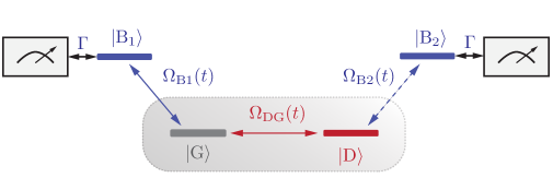
Фигура 6.1: Four-level atom with two counter-steering measurements. Sketch of a modified Darkmon atom consisting of four levels: ground, $\left|\mathrm{G}\right\rangle$, Dark, $\left|\mathrm{D}\right\rangle$, a first ‘‘Bright,’’ $\left|\mathrm{B}_{1}\right\rangle$, and a second ‘‘Bright,’’ $\left|\mathrm{B}_{2}\right\rangle$. Both Bright levels are monitored at rate $\Gamma$, while controlled-actuated Rabi drives $\Omega_{\mathrm{B1}}\left(t\right)$ and $\Omega_{\mathrm{B1}}\left(t\right)$ turn on the effective monitoring of $\left|\mathrm{G}\right\rangle$ and $\left|\mathrm{D}\right\rangle,$ respectively. A potentially stochastic Rabi drive $\Omega_{\mathrm{DG}}\left(t\right)$ links $\left|\mathrm{G}\right\rangle$ and $\left|\mathrm{D}\right\rangle$.

Instead of dissipation engineering, the jump could be reversed by means of a measurement-backaction force due to another measurement. This will likely have to be probabilistic, unless adaptive measurements (Wiseman, 1995, Jacobs, 2003) or measured-based quantum steering is employed (Schrödinger, 1935, Murch et al., 2013b, Wiseman et al., 2007). Specifically, we propose to investigate a four-level scheme that builds on the Darkmon, see Fig. 6.1. The ground state, $\left|\mathrm{G}\right\rangle$, is monitored though a Bright state, $\left|\mathrm{B}_{1}\right\rangle$, by means of Rabi drive, $\Omega_{\mathrm{B1}}\left(t\right)$, and the photodetection of $\left|\mathrm{B}_{1}\right\rangle$ at rate $\Gamma.$ Similarly, the Dark level, $\left|\mathrm{D}\right\rangle$, is monitored by coupling it with a Rabi drive $\Omega_{\mathrm{B2}}\left(t\right)$ to a second Bright state, $\left|\mathrm{B}_{2}\right\rangle$, monitored at rate $\Gamma.$ Conditioned on no clicks, the $\left|\mathrm{G}\right\rangle$ measurement steers the atom toward $\left|\mathrm{D}\right\rangle,$ see Chapter 3. In contrast, conditioned on no clicks, the $\left|\mathrm{D}\right\rangle$ measurement steers the atom toward $\left|\mathrm{G}\right\rangle$. Both forces are phase agnostic. Since they oppose each other, one can be used to undo the effect of the other with proper conditioning and control of the Rabi drives. If $\left|\mathrm{G}\right\rangle$ is measured subject to the Dark Rabi drive $\Omega_{\mathrm{DG}}$ from $\left|\mathrm{G}\right\rangle$ to $\left|\mathrm{D}\right\rangle$, which could be deterministic or stochastic, while $\Omega_{\mathrm{B2}}=0$, the protocol demonstrated in Chapter 1 is implemented. When the signal warning of the occurrence of the quantum jump from $\left|\mathrm{G}\right\rangle$ to $\left|\mathrm{D}\right\rangle$ is detected, $\Omega_{\mathrm{B1}}$ is shut off. If the catch time is set to $\Delta t_{\mathrm{mid}}$, the state of the GD superposition is known to be on the GD equator, but its phase may be unknown. If $\Omega_{\mathrm{B2}}$ is turned on and the record is conditioned on no clicks, the jump should be reversed, no matter what the superposition phase is. More generally, the opposition of the two counter-steering no-click measurements offers a unique testbed for studying non-commuting simultaneous measurements, a topic of rising interest in the field (Jordan and Büttiker, 2005, Ruskov et al., 2010, Hacohen-Gourgy et al., 2016, Perarnau-Llobet and Nieuwenhuizen, 2017, Atalaya et al., 2017, Lewalle et al., 2017, Patti et al., 2017, Ficheux et al., 2018, Chantasri et al., 2018).

Quantum jumps are intimately involved in the detection and correction of errors in quantum information systems (Sun et al., 2013, Ofek et al., 2016). A controller continuously monitors an error syndrome, often parity, such as that of a cavity state (Ofek et al., 2016, Cohen et al., 2017) or multi-qubit stabilizer (Huembeli and Nigg, 2017), and detects jumps in the measurement record, which signal the occurrence of an error. The error needs to corrected. Catch and reversing the quantum jump of an error syndrome prior to its occurrence could prevent the error from manifesting fully. A research direction that could be explored is to couple the GD transition to the parity operator of a long-lived quantum-memory cavity (Kirchmair et al., 2013) that encodes a logical quantum state (Cochrane et al., 1999, Mirrahimi et al., 2014, Leghtas et al., 2015, Michael et al., 2016, Li et al., 2017, Touzard et al., 2018). The parity bit of the cavity state would be continuously mapped onto the GD manifold. The state $\left|\mathrm{G}\right\rangle$ would indicate no error, while $\left|\mathrm{D}\right\rangle$ would indicate that an error has occurred. If the noise process driving the parity bit flips has sufficiently narrow bandwidth, it may be possible to extend the catch and reverse protocol to intervene in the occurrence of the parity-bit error. By monitoring the $\left|\mathrm{B}\right\rangle$/not-$\left|\mathrm{B}\right\rangle$ measurement record as discussed in Chapter 1, the controller would detect the advance-warning signal and immediately perform a phase-agnostic reversal of the jump to prevent the error. Applications of the jump reversal protocol to quantum error correction schemes present an interesting and open direction for theoretical and experimental research.

Closing statement.

We hope the catch and reverse experiment offers a new vantage point on the state-disturbing nature of measurements and the interplay between deterministic forces and the necessarily-stochastic ones due to quantum measurements. More generally, we hope it could provide a conceptually simple but striking illustration to help write operationally-based, rather than postulate-based, textbooks for quantum mechanics.