Correspondence between Phase Oscillator Network and Classical XY Model with the same random and frustrated interactions

Abstract

We study correspondence between a phase oscillator network with distributed natural frequencies and a classical XY model at finite temperatures with the same random and frustrated interactions used in the Sherrington-Kirkpatrick model. We perform numerical calculations of the spin glass order parameter $q$ and the distributions of the local fields. As a result, we find that the parameter dependences of these quantities in both models agree fairly well if parameters are normalized by using the previously obtained correspondence relation between two models with the same other types of interactions. Furthermore, we numerically calculate several quantities such as the time evolution of the instantaneous local field in the phase oscillator network in order to study the roles of synchronous and asynchronous oscillators. We also study the self-consistent equation of the local fields in the oscillator network and XY model derived by the mean field approximation.

PACS numbers

05.45.Xt  05.45.-a  05.20.-y  

I Introduction

The classical XY model which describes magnetism has been studied and a lot of phase transition phenomena have been founddomb.green . On the other hand, there are a lot of synchronization phenomena in nature such as the circadian rhythms, beat of heart, collective firing of fireflies, and so onsaunders ; biological.clocks . For such synchronization phenomena, the phase oscillator model which describes oscillations only by phases has been proposedwinfree , and the synchronization-desynchronization phase transition point has been analytically obtained in the case of the uniform infinite-range interactionkuramoto-1 . The models which are described only by phases are not special in the sense that the differential equations for phases are derived when nonlinear differential equations which exhibit limit cycle oscillations are weakly coupled kuramoto-book . The phase oscillator model with the uniform infinite-range interaction is called the Kuramoto model. Since Kuramoto proposed the model, there have been many extensions of the model, and many interesting phenomena such as chimera states and the synchronization due to common noises have been found, and attempts to identify a dynamical system from experimental data have been maderev.mod.phys .

In the XY model and the phase oscillator network with the same interaction, the order parameters are the same, and it is trivial that the XY model with zero temperature and the phase oscillator network with uniform natural frequencies are equivalent, but previously no relations between these two models have been found beyond this. A few years ago, for a class of infinite-range interactions, we found the correspondence between the XY model with non-zero temperature and the phase oscillator network with distributed natural frequenciesuezu.kimoto.etal . Specifically, temperature $T$ in the XY model corresponds to the width of distribution of natural frequencies in the oscillator network, e.g., $T$ corresponds to $\sqrt{2/\pi}\sigma$ where $\sigma$ is the standard deviation when the distribution is Gaussian. The integration kernels for the saddle point equations (SPEs) for the XY model and the self-consistent equations (SCEs) for the phase oscillator network correspond as well. Furthermore, for several interactions, there exists one-to-one correspondence between solutions for both models, and thus, it is found that the critical exponents are the same in both modelsin preparation .

In what situations correspondence between the two models holds is a very interesting theme. So far, it has been found that correspondence holds when a few order parameters exist and their SPEs and SCEs are derived for a class of infinite-range interactions with or without randomness and without frustration. We have been studying whether correspondence between the two models exists or not for the interactions for which the SPEs and/or SCEs are not derived. In this paper, in particular, we numerically study random frustrated interactions which were used in the Sherrington-Kirkpatrick (SK) modelsk . We call it the Sherrington-Kirkpatrick (SK) interaction in this paper. It is well known that the SK model exhibits the spin glass phase for some parameter range. In the spin glass phase, the total magnetization is zero, but locally each spin is frozen and has non-zero local magnetization. The spins with continuous $n$ components are also studied in Ref. 10), and the SPEs are derived and the spin glass phase is obtained. On the other hand, for the phase oscillator network, more than two decades ago, a numerical study for the SK interaction was performed by Daido and non-trivial behaviors were obtained Daido-1992 . That is, the quasientrainment (QE) state was observed, in which the substantial frequency for each oscillator is very small, but phases between two such oscillators diffuse slowly. Furthermore, the distribution of the local fields (LFs) undergoes a phase transition that the peak position of the distribution changes from zero to non-zero value as a parameter changes and this is called the volcano transition.

In this paper, we perform numerical calculations and study the spin glass order parameter $q$ and distributions of LFs in both models. In addition, in order to study the roles of synchronous and asynchronous oscillators in the phase oscillator network, we numerically calculate several quantities such as the time evolution of the phases of oscillators and local fields, and derive the SCEs of the LFs assuming that only the synchronous oscillators exist. Similarly, in the XY model, by using the naive mean-field approximation, we derive the SCEs of the LFs. We compare theoretical results with numerical ones in both models.

The structure of this paper is as follows. In sect. 2, we formulate the problem and describe the SPEs. In sect. 3, we show the results of numerical simulations. Summary and discussion are given in sect. 4. In Appendix A, we derive the disorder averaged free energy per spin and the SPEs under the ansatz of the replica symmetry in the XY model.

II Formulation

The classical XY model consists of $N$ XY spins $X_{j}=(\cos\phi_{j},\sin\phi_{j}),(j=1,\cdots,N$), where $\phi_{j}$ is the phase of the $j$th XY spin. The Hamiltonian $H$ is given by

$$H=-\sum_{j<k}^{N}J_{jk}\cos(\phi_{j}-\phi_{k}),$$ (1)

where $J_{jk}$ is the interaction between the $j$th and $k$th XY spins. On the other hand, in the phase oscillator network, each oscillator is described by a phase. Let $\phi_{j}$ be the phase of the $j$th phase oscillator. The evolution equation for $\phi_{j}$ is given by

$$\frac{d\phi_{j}}{dt}=\omega_{j}+\sum_{k=1}^{N}J_{jk}\sin(\phi_{k}-\phi_{j}),$$ (2)

where $J_{jk}$ is the interaction from the $k$th to $j$th phase oscillators, the constant $\omega_{j}$ is natural frequency. We assume that $\omega_{j}$ is a random variable generated from the probability density function $g(\omega)$. We assume that $g(\omega)$ is one-humped and symmetric with respect to its center $\omega_{0}$. In this paper, as $g(\omega)$ we adopt the Gaussian distribution with mean 0 and standard deviation $\sigma$, ${\mathcal{N}}(0,\sigma^{2})$. We assume both systems have the following SK interaction in common:

$$J_{jk}=\frac{J}{\sqrt{N}}z_{jk},\\$$ (3)

where $z_{jk}$ is a random variable obeying the Gaussian distribution ${\mathcal{N}}(0,1)$. Moreover, we assume $J_{jj}=0$ and $J_{jk}=J_{kj}(j\neq k)$.

Now, by using the replica method, we derive the saddle point equations (SPEs) for the XY model, which is originally obtained in Ref.sk .

Firstly, in the XY model, we define the following spin glass order parameter $q$:

$$q=\mbox{Max}\left(\left|\frac{1}{N}\sum_{j=1}^{N}e^{i\left(\phi_{j}^{\alpha}-\phi_{j}^{\beta}\right)}\right|,\left|\frac{1}{N}\sum_{j=1}^{N}e^{i\left(\phi_{j}^{\alpha}-(-\phi_{j}^{\beta})\right)}\right|\right),$$ (4)

where $i=\sqrt{-1}$, $\phi_{j}^{\alpha}\ (1\leq j\leq N)$ and $\phi_{j}^{\beta}\ (1\leq j\leq N)$ are phases of two replicas $\alpha$ and $\beta$ that have the same interaction $\{J_{jk}\}$. The first argument is calculated by the phase difference between $\phi_{j}^{\alpha}$ and $\phi_{j}^{\beta}$, and the second argument is calculated by the phase difference between $\phi_{j}^{\alpha}$ and $-\phi_{j}^{\beta}$. Since the Hamiltonian (1) has the reversal symmetry, that is it is invariant under the reversal of signs of phases $\{\phi_{j}\}\to\{-\phi_{j}\}$, we calculate the summation for the reversal phase $-\phi_{j}^{\beta}$ shown in the second argument. Since we set $J_{0}=0$ and $J=1$, then $q>0$ when the system is in the spin glass state, and $q=0$ when it is in the paramagnetic state.

Introducing $n$ replicas, we define the following order parameters. For $\alpha<\beta$,

$$q_{{\rm cc}}^{\alpha\beta}=\frac{1}{N}\sum_{i}\cos\phi_{i}^{\alpha}\cos\phi_{i}^{\beta},\ q_{{\rm ss}}^{\alpha\beta}=\frac{1}{N}\sum_{i}\sin\phi_{i}^{\alpha}\sin\phi_{i}^{\beta},$$ (5)

and for $\alpha\neq\beta$,

$$q_{{\rm cs}}^{\alpha\beta}=\frac{1}{N}\sum_{i}\cos\phi_{i}^{\alpha}\sin\phi_{i}^{\beta},$$ (6)

and for $\alpha=1,\cdots,n$,

$$Q_{{\rm cc}}^{\alpha}=\frac{1}{N}\sum_{i}\cos^{2}\phi_{i}^{\alpha},\ Q_{{\rm ss}}^{\alpha}=\frac{1}{N}\sum_{i}\sin^{2}\phi_{i}^{\alpha},\ Q_{{\rm cs}}^{\alpha}=\frac{1}{N}\sum_{i}\cos\phi_{i}^{\alpha}\sin\phi_{i}^{\alpha}.$$

By using the standard recipe, we obtain the disorder averaged free energy per spin $\bar{f}=-\lim_{N\to\infty}(\beta N)^{-1}\overline{\log Z}$ by the replica method. Here, $\overline{\cdots}$ implies the average over $\{J_{ij}\}$. Assuming the replica symmetry, we obtain

$$\bar{f}_{\rm RS} = -\frac{1}{\beta}\biggl{\{}\frac{\beta^{2}J^{2}}{4}(q_{{\rm cc}}^{2}+q_{{\rm ss}}^{2}+2q_{{\rm cs}}^{2}-Q_{{\rm cc}}^{2}-Q_{{\rm ss}}^{2}-2Q_{{\rm cs}}^{2})$$ (7)

$$+\int Dx\int Dy\log\int d\phi M(\phi|x,y)\biggr{\}},$$

$$M(\phi|x,y) = \exp\biggl{[}\frac{\beta^{2}J^{2}}{2}(Q_{{\rm cc}}-q_{{\rm cc}})\cos^{2}\phi+\frac{\beta^{2}J^{2}}{2}(Q_{{\rm ss}}-q_{{\rm ss}})\sin^{2}\phi$$ (8)

$$+\beta^{2}J^{2}(Q_{{\rm cs}}-q_{{\rm cs}})\sin\phi\cos\phi$$

$$+\beta J\sqrt{\frac{q_{{\rm cc}}q_{{\rm ss}}-(q_{{\rm cs}})^{2}}{q_{{\rm ss}}}}\cos\phi\ x+\beta J\biggl{(}\frac{q_{{\rm cs}}}{\sqrt{q_{{\rm ss}}}}\cos\phi+\sqrt{q_{{\rm ss}}}\sin\phi\biggr{)}y\biggr{]}.$$

From this, we obtain the following SPEs.

$$Q_{{\rm cc}}=[\langle\cos^{2}\phi\rangle],Q_{{\rm ss}}=[\langle\sin^{2}\phi\rangle]=1-Q_{{\rm cc}},\ Q_{{\rm cs}}=[\langle\sin\phi\cos\phi\rangle],$$ (9)

$$q_{{\rm cc}}=[\langle\cos\phi\rangle^{2}],q_{{\rm ss}}=[\langle\sin\phi\rangle^{2}],\ q_{{\rm cs}}=[\langle\sin\phi\rangle\langle\cos\phi\rangle],$$ (10)

$$[\cdots]\equiv\int Dx\int Dy\cdots,\ \langle\cdots\rangle\equiv\frac{\int d\phi M(\phi|x,y)\ \cdots}{\int d\phi M(\phi|x,y)}.$$ (11)

See Appendix A for the derivation. $q$ defined by eq. (4) is rewritten by using these quantities as

$$q = \mbox{ Max }\{\sqrt{(q_{{\rm cc}}^{\alpha\beta}+q_{{\rm ss}}^{\alpha\beta})^{2}+(q_{{\rm sc}}^{\alpha\beta}-q_{{\rm cs}}^{\alpha\beta})^{2}},\sqrt{(q_{{\rm cc}}^{\alpha\beta}-q_{{\rm ss}}^{\alpha\beta})^{2}+(q_{{\rm sc}}^{\alpha\beta}+q_{{\rm cs}}^{\alpha\beta})^{2}}\}.$$ (12)

We found $Q_{\rm cc}=Q_{\rm ss}=\frac{1}{2},Q_{\rm cs}=0$ by the Markov Chain Monte Carlo simulations (MCMCs). As for $q$s, we found several relations among them depending on samples. Assuming $Q_{\rm cc}=Q_{\rm ss}=\frac{1}{2},Q_{\rm cs}=0$, we solved the SPEs for $q_{\rm cc},q_{\rm ss}$, and $q_{\rm cs}$, and obtained $q_{\rm cc}\simeq q_{\rm ss}$ and $q_{\rm cs}\simeq q_{\rm sc}\simeq 0$. By assuming $q_{\rm cc}=q_{\rm ss}$ and $q_{\rm cs}=q_{\rm sc}=0$, we obtain

$$q = 2q_{{\rm cc}}.$$ (13)

In Appendix A, we prove that $q$ obeys the same equation as that derived by Sherrington and Kirkpatricksk ,

$$q = 1-\frac{k_{\rm B}T}{J}\sqrt{\frac{2}{q}}\int_{0}^{\infty}drr^{2}e^{-\frac{1}{2}r^{2}}\frac{I_{1}(\frac{J}{k_{\rm B}T}\sqrt{\frac{q}{2}}r)}{I_{0}(\frac{J}{k_{\rm B}T}\sqrt{\frac{q}{2}}r)},$$ (14)

where $\beta=\frac{1}{k_{\rm B}T}$, $k_{\rm B}$ is the Boltzmann constant, and $I_{n}$ is the $n$th modified Bessel function. The critical temperature is $T_{c}=J/2$ below which the spin glass phase appears.

III Numerical simulation

Here, we show numerical results. In this paper, we set $J_{0}=0$ and $J=1$ and then $T_{c}=0.5$.

III.1 Spin glass order parameter $q$

III.1.1 XY model

Now, let us explain our method of numerical calculations. We use the replica exchange Monte Carlo (REMC) method. We prepared 48 sets and 96 sets of temperature for $N=100$ and 500, respectively, and a replica is assigned to each temperature. We call it a temperature replica. The temperature $T$ ranges from 0.02 to 0.96 with the increment $\Delta T=0.02$ for $N=100$ and $\Delta T=0.01$ for $N=500$, respectively. The initial values of $\{\phi_{j}\}$ of all replicas were set to values in $[0,2\pi)$ randomly. In order to calculate $q$, we prepare another set of replicas. Two sets of replicas are denoted by $\alpha$ and $\beta$, respectively. For $N=100$ (500), we exchange temperature replicas every 5000 (1000) Monte Carlo sweeps (MC sweeps). One MC sweep corresponds to $N$ updates of spins. The number of exchanges is 10000. After 500 exchanges, at each temperature, we calculate the time average of $q$ using 100 sets of phases of XY spins for the last 100 MC sweeps during 5000 and 1000 MC sweeps for $N=100$ and 500, respectively. We denote this average by $\bar{q}$. Then we take the average of $\bar{q}$ over 9500 exchanges, which we regard as the thermal average $\langle q\rangle$. At each temperature, the sample average of $\langle q\rangle$ and its standard deviation are calculated. The number of samples is 30 and 5 for $N=100$ and for $N=500$, respectively. We show the results of the temperature dependence of $q$ in Fig. 1(a) for $N=100$ and in Fig. 1(b) for $N=500$. The solid curves are the theoretical results at the thermodynamic limit of $N=\infty$. The theoretical curves look straight, but they are slightly curved. The black circles are the sample average of $q$ and the error bars are the standard deviation. The theoretical curves and the computer simulation results almost agree with each other at $T<0.3$ for $N=100$, and at $T<0.4$ for $N=500$, respectively. Therefore, it is expected that the agreement between the theoretical curves and the simulation results becomes better as $N$ is increased, and the critical temperature will be $T_{c}=0.5$ which is the theoretical result.

(a)	(b)

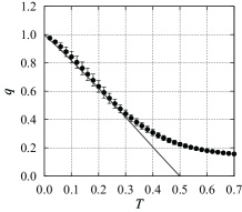
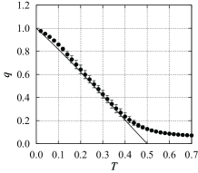
Figure 1: Temperature dependence of sample average of $q$ in XY model. (a) $N=100$, (b) $N=500$.

III.1.2 Phase oscillator network

We adopt the same definition of $q$ by Eq. (4) as in the XY model. In order to guarantee the same reversal symmetry as in the XY model, we generate $\omega_{j}$ for $j=1,2,\cdots,N/2$, and set $\omega_{j}=-\omega_{j-N/2}$ for $j=N/2+1,N/2+2,\cdots,N$. The computer simulation was carried out by the following method. In order to integrate Eq. (2) numerically, we adopt the Euler method with time increment $\Delta t=0.02$. Since the Hamiltonian is not defined for the phase oscillator network, it is impossible to use the REMC method. Therefore, in analogy to the simulated annealing method, the relaxation calculation was carried out while gradually lowering $\sigma$ from $\sqrt{\pi/2}$ to $0$ with the increment $\Delta\sigma=0.01\sqrt{\pi/2}$ for $N=100$, $\Delta\sigma=0.005\sqrt{\pi/2}$ for $N=200$, and $\Delta\sigma=0.001\sqrt{\pi/2}$ for $N=500$. In this paper, we also call this the simulated annealing method. At each $\sigma$, we evolve the system until $t=800$ and calculate the time average of $q$ using phases of oscillators starting from $t=501$ to $t=800$ with time interval 1. We denote this by $\bar{q}$. At each $\sigma$, the sample average of $\bar{q}$, and the standard deviation over samples are calculated. For this simulated annealing method, $\omega_{j}\ (1\leq j\leq N)$ is not generated for every $\sigma$. Instead, firstly, $\omega_{j}$ with $\sigma=1$ is generated according to ${\mathcal{N}}(0,1)$. We denote it $\omega_{j,0}$. Then, $\omega_{j}$ with $\sigma(\neq 1)$ is defined as $\sigma\omega_{j,0}$. The initial values of $\phi_{j}\ (1\leq j\leq N)$ at the beginning of the simulated annealing method are chosen randomly from $[0,2\pi)$. In the simulated annealing method, there may be cases that the relaxed state is captured at a local minimum. In order to judge whether the relaxed state reached the global minimum at $\sigma=0$, we used the fact that the phase oscillator network with $\sigma=0$ and the XY model with $T=0$ are the same model. Concretely, we used the following method. We prepared the same interaction for both models. In the oscillator network, we chose two replicas with $q\simeq 1$ at $\sigma\sim 0$ obtained by the simulated annealing method. Then, we calculated $q$ using $\phi_{j}\ (1\leq j\leq N)$ of one of two replicas of the phase oscillator network at $\sigma\sim 0$ and $\phi_{j}\ (1\leq j\leq N)$ of the XY model at $T=0.02$ obtained by the REMC method. If $q>0.99$, it was judged that the two replicas in the oscillator network reached the global minimum. By this procedure, we obtained 100 ($N=100$), 100 ($N=200$), and 15 ($N=500)$ pairs of replicas which reached the global minimum at $\sigma=0$. From the thus obtained $\bar{q}$s for $\sigma>0$, we calculated the sample average of $q$ and the standard deviation. In Fig. 2, we display the $\sigma$ dependence of the sample average of $q$ with its standard deviation. The solid curve is obtained by the theoretical formula of $q$ for the XY model by setting $\sigma=T\sqrt{\pi/2}$. For $\sigma<0.4$ when $N=100$, $\sigma<0.2$ when $N=200$, and $\sigma<0.17$ when $N=500$, the theoretical curve and the simulation results almost agree. However, contrary to our expectation, as the system size increases, the coinciding range of the theoretical curve and the simulation results decreases. The reason for this is considered that $\phi_{j}$ behaves intermittently in time as we show later. In order to observe the averaged behavior, we introduce the following definition of $q_{\rm av}$ for two replicas $\{\phi_{j}^{\alpha}\}$ and $\{\phi_{j}^{\beta}\}$.

$$q_{\rm av} = {\rm Max}\biggl{(}\frac{|\sum_{j=1}^{N}\bar{A}_{j}^{\alpha}\bar{A}_{j}^{\beta}e^{i(\bar{\phi}_{j}^{\alpha}-\bar{\phi}_{j}^{\beta})}|}{\sum_{j=1}^{N}\bar{A}_{j}^{\alpha}\bar{A}_{j}^{\beta}},\frac{|\sum_{j=1}^{N}\bar{A}_{j}^{\alpha}\bar{A}_{j}^{\beta}e^{i(\bar{\phi}_{j}^{\alpha}+\bar{\phi}_{j}^{\beta})}|}{\sum_{j=1}^{N}\bar{A}_{j}^{\alpha}\bar{A}_{j}^{\beta}}\biggr{)},$$ (16)

$$\bar{A}_{j}^{\alpha}e^{i\bar{\phi}_{j}^{\alpha}}=\frac{1}{T_{s}}\sum_{t}^{T_{s}}e^{i\phi_{j}^{\alpha}(t)},\ \ \bar{A}_{j}^{\beta}e^{i\bar{\phi}_{j}^{\beta}}=\frac{1}{T_{s}}\sum_{t}^{T_{s}}e^{i\phi_{j}^{\beta}(t)},$$

where $T_{s}=300$. The numerical results are shown in Fig. 3 for $N=100,200$, and $N=500$. From this, we note that the order parameter $q_{\rm av}$ for the time averaged phases agree with the theoretical curve fairly well, and as $N$ increases the coinciding range of the theoretical curve and the simulation results increases, and the critical parameter will be $\sigma_{c}=T_{c}\sqrt{\pi/2}$ when $N=\infty$.

(a)	(b)	(c)

Figure 2: $\sigma$ dependence of sample average of $q$ in phase oscillator network. (a) $N=100$, (b) $N=200$, (c) $N=500$.

(a)	(b)	(c)

Figure 3: $\sigma$ dependence of sample average of $q_{\rm av}$ in phase oscillator network. (a) $N=100$, (b) $N=200$, (c) $N=500$.

The results of $T$ dependences of $q$ in the XY model and $\sigma$ dependences of $q$ in the phase oscillator network imply that they differ by the factor $\sqrt{\pi/2}$ in the scale of abscissa axes as expected.

III.2 Local Field

Now, let us study the local field $p_{j}=x_{j}+i\;y_{j}$ which is defined by

$$p_{j}=\sum_{k=1}^{N}J_{jk}\;e^{i\phi_{k}}.$$ (17)

LFs move on the complex plane with time due to the thermal fluctuation in the XY model, and in the phase oscillator network they move on the complex plane with time according to the evolution equation (2).

III.2.1 XY model

We numerically examined the spatial distribution of LFs on the complex plane for all spins. The initial values of $\phi_{j}\ (1\leq j\leq N)$ were set as the final equilibrium state obtained when we calculated $q$. In Fig. 4, we display the distribution of LFs on the complex plane and the probability density $P(r)$ of LFs, where $r=\sqrt{x^{2}+y^{2}}$. To draw Fig. 4, a Monte Carlo simulation was carried out for $N=500$ and data were taken every 1 MC sweep during 10000 MC sweeps. That is, $10000\times N$ data are used to draw Fig. 4. When $T$ is low, $P(r)$ is a volcanic shape with a hole in the center, i.e., $r=0$, and the hole gradually closes with the increase of $T$, and then it disappears and the peak position becomes $r=0$ for $T>0.5(=T_{c})$.

(a)	(b)
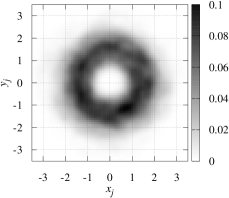
(c)	(d)
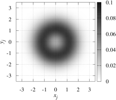
(e)	(f)
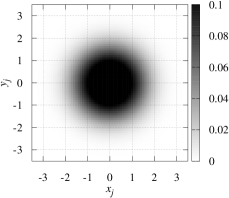
(g)	(h)

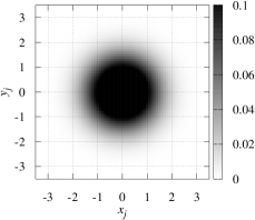
Figure 4: Local field of XY model ($N=500$). Left panel: spatial distribution of LFs on the complex plane. Right panel: probability density of LFs, $P(r)$. (a), (b) $T=0.04$, (c), (d) $T=0.26$, (e), (f) $T=0.5$, (g), (h) $T=0.6$.

III.2.2 Phase oscillator network

We calculated LFs as in the XY model. The initial values of $\phi_{j}\ (1\leq j\leq N)$ were set as the final state obtained when we calculated $q$. In Fig. 5, we display the distribution of LFs and $P(r)$. A computer simulation was carried out for $N=500$ until $t=10000$, and data were taken every time interval 1 to draw Fig. 5. That is, the number of data to draw Fig. 5 is the same as in the XY model. As is seen from Fig. 5, with the increase of $\sigma$ from 0, behavior of $P(r)$ is the same as in the XY model and the peak position becomes $r=0$ for $\sigma>0.5\sqrt{\pi/2}(=T_{c}\sqrt{\pi/2})$.

(a)	(b)
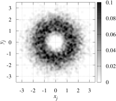
(c)	(d)
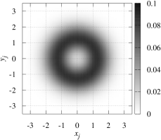
(e)	(f)
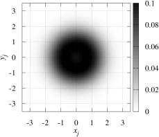
(g)	(h)

Figure 5: Local field of phase oscillator network ($N=500$). Left panel: spatial distribution on the complex plane. Right panel: probability density $P(r)$. (a), (b) $T=0.04\sqrt{\pi/2}$, (c), (d) $T=0.26\sqrt{\pi/2}$, (e), (f) $T=0.5\sqrt{\pi/2}$, (g), (h) $T=0.6\sqrt{\pi/2}$.

III.2.3 Comparison of results for both models

In the LFs of the XY model, for $N=500$, the $T$ dependence of the radius at which the probability density has a peak is shown in Fig. 6(a). We call the radius the peak radius, and denote it by $r_{p}$. The black circles show the peak radius, and the error bars show the radius at which the probability density decreases by 5% from the peak. The peak radius at $T>0.5(=T_{c})$ becomes nearly zero. In the LFs of the phase oscillator network, for $N=500$, the $\sigma$ dependence of the peak radius is shown in Fig. 6(b). The circles and error bars have the same meanings as in the XY model. The peak radius at $\sigma>0.5\sqrt{\pi/2}(=T_{c}\sqrt{\pi/2})$ becomes nearly zero. $T$ and $\sigma$ in which the peak radius becomes zero seem to differ by the factor $\sqrt{\pi/2}$ in the scale of abscissa axes as expected.

(a)	(b)

Figure 6: Temperature dependence of the peak radius $r_{p}$ in the XY model ($N=500$) and $\sigma$ dependence of $r_{p}$ in the phase oscillator network ($N=500$). (a) XY model, (b) phase oscillator

(a)

(b)

(c)

Figure 7: Time series of $\sin\phi(t)$. $N=100$. (a) $J_{jk}=0$, (b) $J_{jk}\neq 0,\sigma=0.2$, (c) $J_{jk}\neq 0,\sigma=0.3$.

III.3 Numerical results for several quantities in the phase oscillator network

In the phase oscillator network, in order to study the roles of synchronous and asynchronous oscillators for the correspondence, we numerically calculated several quantities. Firstly, we study the time evolution of $\sin\phi$ where $\phi$ is the phase of each oscillator. In Fig. 7, we show $\sin\phi(t)$ of 20 oscillators for $N=100$ during $t=0\sim 150$. In Fig. 7(a), we set $J_{jk}=0$, that is, $\phi_{j}=\omega_{j}t+\phi_{j}(0)$. In Figs. 7(b) and (c), we set $J_{jk}\neq 0$, and $\sigma=0.2\sqrt{\frac{\pi}{2}}$ and $0.3\sqrt{\frac{\pi}{2}}$, respectively. We note that oscillators are locked for a while and then are unlocked, and repeat this behavior. We found that the larger $\sigma$ is, the more fluctuations of phases are, and trajectories behave chaotically. Next, we studied trajectories of LFs for a long time, from 0 to 2000 for $N=100\sim 400$. See Figs. (8) and (9). We define the amplitude $R_{j}$ and phase $\Theta_{j}$ of the LFs by

$$R_{j}e^{i\Theta_{j}} = p_{j}=\sum_{k}J_{jk}e^{i\phi_{k}}.$$ (18)

In this simulation, we adopted the simulated annealing and the schedule is $T_{l}=0.7-(l-1)*0.02,l=1\sim 35$. We obtained the following results. When $\sigma$ is small, $\sigma<\sigma_{c1}$, $R_{j}$ and $\Theta_{j}$ are constant or periodic depending on $N$, where $\sigma_{c}\sim 0.1\sqrt{\frac{\pi}{2}}$. The distribution of substantial frequencies is $G(\tilde{\omega})=\delta(\tilde{\omega})$. When $\sigma$ is large, $R_{j}$ behaves chaotically, and $\Theta_{j}$ has two phases, in one phase $\Theta_{j}$ is almost constant, and in the other phase it increases or decreases drastically. On average, $\Theta_{j}$ evolves almost linearly. $G(\tilde{\omega})$ is one humped, continuous, and it is impossible to separate synchronized oscillators from desynchronized ones.

In the next subsection, we derive the self-consistent equations for LFs in the XY model and oscillator network by using approximations.

Figure 8: Time series of $R_{j}$s for several oscillators. $N=100$. (a) $\sigma=0.1\sqrt{0.5\pi}$, (b) $\sigma=0.2\sqrt{0.5\pi}$, (c) $\sigma=0.3\sqrt{0.5\pi}$, (d) $\sigma=0.5\sqrt{0.5\pi}$.

Figure 9: Time series of $\Theta_{j}$s for several oscillators. $N=100$. (a) $\sigma=0.1\sqrt{0.5\pi}$, (b) $\sigma=0.2\sqrt{0.5\pi}$, (c) $\sigma=0.3\sqrt{0.5\pi}$, (d) $\sigma=0.5\sqrt{0.5\pi}$.

III.4 SCE for LFs

In the oscillator network, we derive the SCE for the case that all oscillators are synchronized. In the XY model, we derive the SCE by using the naive mean-field approximation.

III.4.1 Oscillator network

Using $R_{j}$ and $\Theta_{j}$, the evolution equation is rewritten as

$$\frac{d}{dt}\phi_{j} = \omega_{j}-R_{j}\sin(\phi_{j}-\Theta_{j}).$$ (19)

$R_{j}$ and $\Theta_{j}$ are constant because all oscillators are assumed to be synchronized. Thus, by defining $\psi_{j}=\phi_{j}-\Theta_{j}$, we obtain

$$\frac{d}{dt}\psi_{j} = \omega_{j}-R_{j}\sin\psi_{j}.$$ (20)

The stable solution is $\psi_{j}^{*}=\sin^{-1}\frac{\omega_{j}}{R_{j}}$ where $|\psi_{j}^{*}|<\frac{\pi}{2}$. The probability density function of phases $f(\psi;\omega_{j})$ is $\delta(\psi-\psi_{j}^{*})$. Thus, the average of $e^{i\phi_{j}}$ is

$$\langle e^{i\phi_{j}}\rangle = e^{i(\psi_{j}^{*}+\Theta_{j})}=\biggl{(}\sqrt{1-(\frac{\omega_{j}}{R_{j}})^{2}}+i\frac{\omega_{j}}{R_{j}}\biggr{)}e^{i\Theta_{j}}.$$ (21)

Therefore, the SCE for LFs is

$$R_{j}e^{i\Theta_{j}} = \sum_{j^{\prime}=1}^{N}J_{jj^{\prime}}\biggl{(}\sqrt{1-(\frac{\omega_{j^{\prime}}}{R_{j^{\prime}}})^{2}}+i\frac{\omega_{j^{\prime}}}{R_{j^{\prime}}}\biggr{)}e^{i\Theta_{j^{\prime}}}.$$ (22)

We numerically solved the SCE (22) by iteration method. That is, from $\{R_{j}\}$ and $\{\Theta_{j}\}$ at time $t$, we evaluate the right-hand side of eq. (22) to obtain $\{R_{j}\}$ and $\{\Theta_{j}\}$ at time $t+\Delta t$. We define the distance between two configurations $\{\phi_{j}\}$ and $\{\phi_{j}^{\prime}\}$ as

$$d(\{\phi_{j}\},\{\phi_{j}^{\prime}\})\equiv\sum_{j=1}^{N}|\phi_{j}-\phi_{j}^{\prime}|.$$

The convergence condition is $d(\{\phi_{j}(t)\},\{\phi_{j}(t+\Delta t)\})<\epsilon$ for successive two configurations $\{\phi_{j}(t)\}$ and $\{\phi_{j}(t+\Delta t)\}$ with $\epsilon=0.01$. It turned out that it is very difficult to obtain solutions for eq. (22) if initial conditions are taken randomly. Then, as an initial condition, we used the numerical results obtained by the simulated annealing method, and found that almost all numerical results are solutions of the SCE when $\sigma$ is small. For example, we found that when $N=100$ and $\sigma=0.02\sqrt{\frac{\pi}{2}}$, all 19 configurations obtained by the simulated annealing converge by only one iteration and $d(\{\phi_{j}(0)\},\{\phi_{j}(\Delta t)\})\sim 3\times 10^{-5}$, that is, these configurations satisfy eq. (22). We regard two configurations $\{\phi_{j}\}$ and $\{\phi_{j}^{\prime}\}$ to be different when $d(\{\phi_{j}\},\{\phi_{j}^{\prime}\})>\epsilon$. We found only two different configurations among 19 configurations. When $N=100$ and $\sigma=0.1\sqrt{\frac{\pi}{2}}$, we found that 16 configurations converge by only one iteration among 19 configurations, and all of them are regarded as the same. However, for larger values of $\sigma$, we could not find any solution. This is because $R_{j}$ and $\Theta_{j}$ are not constant and it seems that asynchronous solutions contribute to the LFs.

III.4.2 XY model

Hamiltonian is

$$H = -\sum_{j<k}J_{jk}\cos(\phi_{k}-\phi_{j})=-\frac{1}{2}\sum_{j}R_{j}\cos(\phi_{j}-\Theta_{j}).$$ (23)

Since the probability density function of phases is $P(\phi_{j})=\frac{e^{\beta R_{j}\cos(\phi_{j}-\Theta_{j})}}{2\pi I_{0}(\beta R_{j})}$, defining $\psi_{j}=\phi_{j}-\Theta_{j}$ we obtain

$$\langle e^{i\phi_{j}}\rangle = \frac{1}{2\pi I_{0}(\beta R_{j})}\int_{0}^{2\pi}e^{\beta R_{j}\cos\psi}e^{i(\psi+\Theta_{j})}d\phi$$ (24)

$$= \frac{I_{1}(\beta R_{j})}{I_{0}(\beta R_{j})}e^{i\Theta_{j}}=\beta R_{j}e^{i\Theta_{j}}u(\beta R_{j}).$$

Here, $u(x)=\frac{I_{1}(x)}{xI_{0}(x)}$. Thus, we obtain

$$R_{j}e^{i\Theta_{j}} = \sum_{k}J_{jk}\langle e^{i\phi_{k}}\rangle=\beta\sum_{k}J_{jk}R_{k}e^{i\Theta_{k}}u(\beta R_{k}).$$ (25)

As an initial condition, we used the configuration obtained by the simulated annealing as in the oscillator network. The method to solve eq. (25), the convergence condition, and the criterion of different solutions are the same as in the phase oscillator network. When $N=100$ and $T=0.02$, among 30 configurations, 3 configurations converge with $\epsilon=0.01$. The numbers of iterations are rather large compared to the oscillator network, and are 29, 51, and 62 for these three configurations, respectively. All of them are different, but it is difficult to distinguish these three from the figure of $j$ vs. $R_{j}$. When $N=100$ and $T=0.1$, among 30 configurations, 5 configurations converge, and the number of iterations ranges from 50 to 70. Four configurations among 5 are different. We found that convergent values and initial conditions are rather different and this is consistent with the fact that the numbers of iterations are large. See Fig. 10. Therefore, in this case, final configurations by the simulated annealing for $T=0.1$ are not considered as the solutions of the SCEs. The reason for this is considered that the naive mean field approximation is not valid for the high temperatures.

Figure 10: $j$ dependences of $R_{j}$. XY model. $N=100$. Symbols: different solutions among convergent solutions obtained by the iteration of eq. (25), broken line: initial condition which is the final value of the annealing. (a) $T=0.02$, 3 different solutions. (b) $T=0.1$, 4 different solutions.

IV Summary and discussion

We summarize the results of this paper. We studied the random and frustrated interaction, the SK interaction, which is generated by the Gaussian distribution with mean 0 and standard deviation $J/\sqrt{N}$. As for the distribution of natural frequencies $g(\omega)$, we adopted the Gaussian distribution with mean 0 and standard deviation $\sigma$. In order to study whether correspondence between the two models exists or not, we performed numerical calculations of the spin glass order parameter $q$ and the distributions of local fields (LFs) in the XY model and phase oscillator network. In the XY model, we used the Markov Chain Monte Carlo simulation (MCMCs), in particular, the replica exchange Monte Carlo (REMC) method and the simulated annealing method. In the oscillator network, we used the Euler method with time increment $\Delta t=0.02$, and also used the simulated annealing method, that is, we integrate the evolution equation by decreasing $\sigma$ slowly. First, we summarize the results of $q$. In the XY model, we confirmed that theoretical and numerical results agree fairly well and found that the coinciding region between the theoretical curve and the simulation results of $q$ increases as $N$ increases. For the phase oscillator network, we found that in the $\sigma$ dependence of the spin glass order parameter the coinciding region between the theoretical curve $q(T(\sigma))$ of the XY model and the simulation results decreases as $N$ increases, contrary to our expectation. Here, $T(\sigma)=\sqrt{\frac{2}{\pi}}\sigma$ is the relation obtained in the previous paper. Since $\phi_{j}$ behaves intermittently in time, we introduced the order parameter $q_{\rm av}$ for the time averaged phases, and found that the coinciding region between the theoretical curve of the XY model and the simulation results of $q_{\rm av}$ increases as $N$ increases.
Next, we summarize the results of LFs. We define the probability density $P(r)$ of LFs, where $r$ is the radius of the local field in the complex plane. As $T$ or $\sigma$ increases, the peak radius $r_{p}$ of $P(r)$ changes from non-zero value to 0. This is the so called volcano transition, and the transition points of the two models seem to correspond according to the relation $T=\sqrt{\frac{2}{\pi}}\sigma$. For the oscillator network, we numerically studied time evolution of $\sin\phi_{i}$ of each oscillator and found that oscillators are locked for a while and then are unlocked, and repeat this behavior. We also numerically studied time evolution amplitudes $R$s and phases $\Theta$s of LFs. We found that when $\sigma$ is small, they are constant or periodic depending on $N$, and the distribution of the substantial frequencies $G(\omega)$ is the delta function $\delta(\omega)$, but when $\sigma$ is large, $R_{j}$ behaves chaotically, and $\Theta_{j}$ has two phases, in one phase $\Theta_{j}$ is almost constant, and in the other phase it increases or decreases drastically. On average, $\Theta_{j}$ evolves almost linearly. $G(\omega)$ is one-humped and continuous.
Finally, we derived the self-consistent equation (SCE) of LFs for the oscillator network in the case that all oscillators synchronize, and for the XY model by using the naive mean field approximation. We found that for the oscillator network and XY model, when $\sigma$ and $T$ are small, configurations obtained by simulated annealing satisfy the SCE, but when $\sigma$ and $T$ are large, they do not. The reasons for the discrepancy between theoretical and numerical results for the LFs at large $T$ and $\sigma$ are considered as follows. In the oscillator network, the asynchronous oscillators do not contribute to the LFs for the solvable models when the $g(\omega)$ is one-humped and symmetric with respect to its center. However, the present results imply that asynchronous oscillators contribute to the LFs. Since $G(\omega)$ is continuous, it is difficult to separate synchronized oscillators from desynchronized ones. In the XY model, the present results imply that the naive mean-field approximation is not valid except for very low temperatures. This is the same as in the case of Ising spins. The so called Onsager reaction field should be taken into account for the XY model as in the Ising model. Therefore, in order to improve the present approximations for the two models, further elaborate studies are necessary, and these studies are beyond the scope of the present paper and are left as a future problem.

The present study is supported by JPSJ KAKENHI Grant No. 16K05474, No. 25330298, No. 17K00357.

V Appendix A

In this appendix, we derive the disorder averaged free energy per spin and the SPEs under the ansatz of the replica symmetry. The derivation is based on Ref. Hatchett.Uezu.2008

$$\bar{f} = -\lim_{N\to\infty}\lim_{n\to 0}(\beta Nn)^{-1}\log\int d{\mbox{\boldmath$\phi$}}^{1}\cdots{\mbox{\boldmath$\phi$}}^{n}\overline{e^{-\beta\sum_{\alpha}H({\mbox{\boldmath$\phi$}}^{\alpha})}},$$ (26)

$$\overline{e^{-\beta\sum_{\alpha}H({\mbox{\boldmath$\phi$}}^{\alpha})}} = \exp[\frac{\beta^{2}J^{2}}{4N}\sum_{\alpha\beta}\{(\sum_{i}\cos\phi_{i}^{\alpha}\cos\phi_{i}^{\beta})^{2}+(\sum_{i}\cos\phi_{i}^{\alpha}\sin\phi_{i}^{\beta})^{2}$$ (27)

$$+(\sum_{i}\cos\phi_{i}^{\alpha}\sin\phi_{i}^{\beta})^{2}+(\sum_{i}\sin\phi_{i}^{\alpha}\cos\phi_{i}^{\beta})^{2}+-N\}],$$

where ${\mbox{\boldmath$\phi$}}^{\alpha}=(\phi_{1}^{\alpha},\cdots,\phi_{N}^{\alpha})$. We define the following order parameters. For $\alpha<\beta$,

$$q_{{\rm cc}}^{\alpha\beta}=\frac{1}{N}\sum_{i}\cos\phi_{i}^{\alpha}\cos\phi_{i}^{\beta},\ q_{{\rm ss}}^{\alpha\beta}=\frac{1}{N}\sum_{i}\sin\phi_{i}^{\alpha}\sin\phi_{i}^{\beta},$$

$$q_{{\rm cs}}^{\alpha\beta}=\frac{1}{N}\sum_{i}\cos\phi_{i}^{\alpha}\sin\phi_{i}^{\beta},\ q_{{\rm sc}}^{\alpha\beta}=\frac{1}{N}\sum_{i}\sin\phi_{i}^{\alpha}\cos\phi_{i}^{\beta},$$

and for $\alpha=1,\cdots,n$,

$$Q_{{\rm cc}}^{\alpha}=\frac{1}{N}\sum_{i}\cos^{2}\phi_{i}^{\alpha},\ Q_{{\rm ss}}^{\alpha}=\frac{1}{N}\sum_{i}\sin^{2}\phi_{i}^{\alpha},\ Q_{{\rm cs}}^{\alpha}=\frac{1}{N}\sum_{i}\cos\phi_{i}^{\alpha}\sin\phi_{i}^{\alpha}.$$

Then, we obtain

$$\overline{e^{-\beta\sum_{\alpha}H({\mbox{\boldmath$\phi$}}^{\alpha})}} = e^{-\frac{\beta^{2}J^{2}n^{2}}{4}}\exp[\frac{\beta^{2}J^{2}N}{4}\sum_{\alpha}\{(Q_{{\rm cc}}^{\alpha})^{2}+(Q_{{\rm ss}}^{\alpha})^{2}+2(Q_{{\rm cs}}^{\alpha})^{2}\}$$ (28)

$$+2\sum_{\alpha<\beta}\{(q_{{\rm cc}}^{\alpha\beta})^{2}+(q_{{\rm ss}}^{\alpha\beta})^{2}+(q_{{\rm cs}}^{\alpha\beta})^{2}+(q_{{\rm sc}}^{\alpha\beta})^{2}\}].$$

Using the integral representation of $\delta$ functions such as

$$\int\frac{1}{2\pi}dq_{{\rm cc}}^{\alpha\beta}d\hat{q}_{{\rm cc}}^{\alpha\beta}e^{i\hat{q}_{{\rm cc}}^{\alpha\beta}(q_{{\rm cc}}^{\alpha\beta}-\frac{1}{N}\sum_{i}\cos\phi_{i}^{\alpha}\cos\phi_{i}^{\beta})}=1,$$

and re-scaling variables as $\hat{q}_{{\rm cc}}^{\alpha\beta}\to N\hat{q}_{{\rm cc}}^{\alpha\beta}$, $\hat{Q}_{{\rm cc}}^{\alpha}\to N\hat{Q}_{{\rm cc}}^{\alpha}$, etc., we obtain

$$\bar{f} = -\lim_{N\to\infty}\lim_{n\to 0}(\beta Nn)^{-1}\log\{\int d{\mbox{\boldmath$q$}}e^{N(\Phi+\Psi)}\},$$ (29)

$$\Phi = i\sum_{\alpha}\{\hat{Q}_{{\rm cc}}^{\alpha}Q_{{\rm cc}}^{\alpha}+\hat{Q}_{{\rm ss}}^{\alpha}Q_{{\rm ss}}^{\alpha}+\hat{Q}_{{\rm cs}}^{\alpha}Q_{{\rm cs}}^{\alpha}\}+i\sum_{\alpha<\beta}\{\hat{q}_{{\rm cc}}^{\alpha\beta}q_{{\rm cc}}^{\alpha\beta}+\hat{q}_{{\rm ss}}^{\alpha\beta}q_{{\rm ss}}^{\alpha\beta}+\hat{q}_{{\rm cs}}^{\alpha\beta}+\hat{q}_{{\rm sc}}^{\alpha\beta}\}$$

$$+\frac{\beta^{2}J^{2}}{4}\biggl{\{}\sum_{\alpha}\biggl{(}(Q_{{\rm cc}}^{\alpha})^{2}+(Q_{{\rm ss}}^{\alpha})^{2}+2(Q_{{\rm cs}}^{\alpha})^{2}\biggr{)}+2\sum_{\alpha<\beta}\biggl{(}(q_{{\rm cc}}^{\alpha\beta})^{2}+(q_{{\rm ss}}^{\alpha\beta})^{2}+(q_{{\rm cs}}^{\alpha\beta})^{2}+(q_{{\rm sc}}^{\alpha\beta})^{2}\biggr{)}\biggr{\}},$$

$$\Psi = \frac{1}{N}\log\biggl{\{}[\int\prod_{\alpha}d{\mbox{\boldmath$\phi$}}^{\alpha}]$$

$$\times\exp[-i\sum_{\alpha}\sum_{i}(\hat{Q}_{{\rm cc}}^{\alpha\beta}\cos^{2}\phi_{i}^{\alpha}+\hat{Q}_{{\rm ss}}^{\alpha\beta}\sin^{2}\phi_{i}^{\alpha}+\hat{Q}_{{\rm cs}}^{\alpha\beta}\cos\phi_{i}^{\alpha}\sin\phi_{i}^{\alpha})$$

$$-i\sum_{\alpha<\beta}\sum_{i}(\hat{q}_{{\rm cc}}^{\alpha\beta}\cos\phi_{i}^{\alpha}\cos\phi_{i}^{\beta}+\hat{q}_{{\rm ss}}^{\alpha\beta}\sin\phi_{i}^{\alpha}\sin\phi_{i}^{\beta}+\hat{q}_{{\rm cs}}^{\alpha\beta}\cos\phi_{i}^{\alpha}\sin\phi_{i}^{\beta}+\hat{q}_{{\rm sc}}^{\alpha\beta}\sin\phi_{i}^{\alpha}\cos\phi_{i}^{\beta}]\biggr{\}},$$

where $d{\mbox{\boldmath$q$}}=\prod_{\alpha}\biggl{(}\frac{Nd\hat{Q}_{{\rm cc}}^{\alpha}dQ_{{\rm cc}}^{\alpha}}{2\pi}\frac{Nd\hat{Q}_{{\rm ss}}^{\alpha}dQ_{{\rm ss}}^{\alpha}}{2\pi}\frac{Nd\hat{Q}_{{\rm cs}}^{\alpha}dQ_{{\rm cs}}^{\alpha}}{2\pi}\biggr{)}\prod_{\alpha<\beta}\biggl{(}\frac{Nd\hat{q}_{{\rm cc}}^{\alpha\beta}dq_{{\rm cc}}^{\alpha\beta}}{2\pi}\frac{Nd\hat{q}_{{\rm ss}}^{\alpha\beta}dq_{{\rm ss}}^{\alpha\beta}}{2\pi}\frac{Nd\hat{q}_{{\rm cs}}^{\alpha\beta}dq_{{\rm cs}}^{\alpha\beta}}{2\pi}\frac{Nd\hat{q}_{{\rm sc}}^{\alpha\beta}dq_{{\rm cs}}^{\alpha\beta}}{2\pi}\biggr{)}$. Since we consider $N\to\infty$, the integration is estimated by the saddle point of $\Phi+\Psi$,

$$\bar{f} = -\lim_{N\to\infty}\lim_{n\to 0}(\beta Nn)^{-1}\log\{\int d{\mbox{\boldmath$q$}}e^{N(\Phi+\Psi)}\}\sim-\lim_{n\to 0}(\beta n)^{-1}\mbox{ extr }(\Phi+\Psi).$$ (31)

Now, let us consider the replica symmetric solution.

$$Q_{{\rm cc}}^{\alpha}=Q_{{\rm cc}},\ Q_{{\rm ss}}^{\alpha}=Q_{{\rm ss}},\ Q_{{\rm cs}}^{\alpha}=Q_{{\rm cs}},\ \hat{Q}_{{\rm cc}}^{\alpha}=\hat{Q}_{{\rm cc}},\ \hat{Q}_{{\rm ss}}^{\alpha}=\hat{Q}_{{\rm ss}},\ \hat{Q}_{{\rm cs}}^{\alpha}=\hat{Q}_{{\rm cs}},$$ (32)

$$q_{{\rm cc}}^{\alpha\beta}=q_{{\rm cc}},\ q_{{\rm ss}}^{\alpha\beta}=q_{{\rm ss}},\ q_{{\rm cs}}^{\alpha\beta}=q_{{\rm cs}},\ \hat{q}_{{\rm cc}}^{\alpha\beta}=\hat{q}_{{\rm cc}},\ \hat{q}_{{\rm ss}}^{\alpha\beta}=\hat{q}_{{\rm ss}},\ \hat{q}_{{\rm cs}}^{\alpha\beta}=\hat{q}_{{\rm cs}},\hat{q}_{{\rm sc}}^{\alpha\beta}=\hat{q}_{{\rm sc}}.$$

Then , by changing conjugate variables from $\hat{q}_{{\rm cc}}\to i\hat{q}_{{\rm cc}},\hat{Q}_{{\rm cc}}\to i\hat{Q}_{{\rm cc}}$, etc., we obtain

$$\lim_{n\to 0}\frac{1}{n}\Phi_{\rm RS} = -(\hat{Q}_{{\rm cc}}Q_{{\rm cc}}+\hat{Q}_{{\rm ss}}Q_{{\rm ss}}+\hat{Q}_{{\rm cs}}Q_{{\rm cs}})+\frac{1}{2}(\hat{q}_{{\rm cc}}q_{{\rm cc}}+\hat{q}_{{\rm ss}}q_{{\rm ss}}+\hat{q}_{{\rm cs}}q_{{\rm cs}}+\hat{q}_{{\rm sc}}q_{{\rm sc}})$$ (34)

$$+\frac{\beta^{2}J^{2}}{4}(Q_{{\rm cc}}^{2}+Q_{{\rm ss}}^{2}+2Q_{{\rm cs}}^{2}-q_{{\rm cc}}^{2}-q_{{\rm ss}}^{2}-q_{{\rm cs}}^{2}-q_{{\rm sc}}^{2}),$$

$$\lim_{n\to 0}\frac{1}{n}\Psi_{\rm RS} = \lim_{n\to 0}\frac{1}{n}\log(\int[\prod_{\alpha}d\phi^{\alpha}]e^{L}),$$ (35)

$$L = \sum_{\alpha}(\hat{Q}_{{\rm cc}}\cos^{2}\phi^{\alpha}+\hat{Q}_{{\rm ss}}\sin^{2}\phi^{\alpha}+\hat{Q}_{{\rm cs}}\cos\phi^{\alpha}\sin\phi^{\alpha})$$

$$+\sum_{\alpha<\beta}(\hat{q}_{{\rm cc}}\cos\phi^{\alpha}\cos\phi^{\beta}+\hat{q}_{{\rm ss}}\sin\phi^{\alpha}\sin\phi^{\beta}+\hat{q}_{{\rm cs}}\cos\phi^{\alpha}\sin\phi^{\beta}+\hat{q}_{{\rm sc}}\sin\phi^{\alpha}\cos\phi^{\beta}).$$

By using the Hubbard-Stratonovich transformation, $e^{L}$ is rewritten as

$$e^{L} = \exp[\biggl{(}\hat{Q}_{{\rm cc}}-\frac{1}{2}\hat{q}_{{\rm cc}}\biggr{)}\sum_{\alpha}\cos^{2}\phi^{\alpha}+\biggl{(}\hat{Q}_{{\rm ss}}-\frac{1}{2}\hat{q}_{{\rm ss}}\biggr{)}\sum_{\alpha}\sin^{2}\phi^{\alpha}$$

$$+\biggl{(}\hat{Q}_{{\rm cs}}-\frac{\hat{q}_{{\rm cs}}+\hat{q}_{{\rm sc}}}{2}\biggr{)}\sum_{\alpha}\sin\phi^{\alpha}\cos\phi^{\alpha}]$$

$$\times\int Dx\int Dy$$

$$\times\exp[\sqrt{\frac{\hat{q}_{{\rm c}}\hat{q}_{{\rm ss}}-(\frac{\hat{q}_{{\rm cs}}+\hat{q}_{{\rm cs}}}{2})^{2}}{\hat{q}_{{\rm ss}}}}\sum_{\alpha}\cos\phi^{\alpha}\ x+\biggl{(}\frac{(\hat{q}_{{\rm cs}}+\hat{q}_{{\rm sc}})}{2\sqrt{\hat{q}_{{\rm ss}}}}\sum_{\alpha}\cos\phi^{\alpha}+\sqrt{\hat{q}_{{\rm ss}}}\sum_{\alpha}\sin\phi^{\alpha}\biggr{)}y],$$

Then, we obtain

$$\lim_{n\to 0}\frac{1}{n}\Psi_{\rm RS} = \int Dx\int Dy\log\int d\phi\exp\biggl{[}\biggl{(}\hat{Q}_{{\rm cc}}-\frac{1}{2}\hat{q}_{{\rm cc}}\biggr{)}\cos^{2}\phi+\biggl{(}\hat{Q}_{{\rm ss}}-\frac{1}{2}\hat{q}_{{\rm ss}}\biggr{)}\sin^{2}\phi$$

$$+\biggl{(}\hat{Q}_{{\rm cs}}-\frac{\hat{q}_{{\rm cs}}+\hat{q}_{{\rm sc}}}{2}\biggr{)}\sin\phi\cos\phi$$

$$+\sqrt{\frac{\hat{q}_{{\rm c}}\hat{q}_{{\rm ss}}-(\frac{\hat{q}_{{\rm cs}}+\hat{q}_{{\rm cs}}}{2})^{2}}{\hat{q}_{{\rm ss}}}}\cos\phi\ x+\biggl{(}\frac{\hat{q}_{{\rm cs}}+\hat{q}_{{\rm sc}}}{2\sqrt{\hat{q}_{{\rm ss}}}}\cos\phi+\sqrt{\hat{q}_{{\rm ss}}}\sum_{\alpha}\sin\phi\biggr{)}y\biggr{]}.$$

$\bar{f}_{\rm RS}$ is expressed as

$$\bar{f}_{\rm RS} = -\frac{1}{\beta}\lim_{n\to 0}\frac{1}{n}(\Phi_{\rm RS}+\Psi_{\rm RS})$$

$$= -\frac{1}{\beta}\biggl{\{}-(\hat{Q}_{{\rm cc}}Q_{{\rm cc}}+\hat{Q}_{{\rm ss}}Q_{{\rm ss}}+\hat{Q}_{{\rm cs}}Q_{{\rm cs}})+\frac{1}{2}(\hat{q}_{{\rm cc}}q_{{\rm cc}}+\hat{q}_{{\rm ss}}q_{{\rm ss}}+\hat{q}_{{\rm cs}}q_{{\rm cs}}+\hat{q}_{{\rm sc}}q_{{\rm sc}})$$

$$+\frac{\beta^{2}J^{2}}{4}(Q_{{\rm cc}}^{2}+Q_{{\rm ss}}^{2}+2Q_{{\rm cs}}^{2}-q_{{\rm cc}}^{2}-q_{{\rm ss}}^{2}-q_{{\rm cs}}^{2}-q_{{\rm ss}}^{2}),$$

$$+\int Dx\int Dy\log\int d\phi\exp\biggl{[}\biggl{(}\hat{Q}_{{\rm cc}}-\frac{1}{2}\hat{q}_{{\rm cc}}\biggr{)}\cos^{2}\phi+\biggl{(}\hat{Q}_{{\rm ss}}-\frac{1}{2}\hat{q}_{{\rm ss}}\biggr{)}\sin^{2}\phi$$

$$+\biggl{(}\hat{Q}_{{\rm cs}}-\frac{\hat{q}_{{\rm cs}}+\hat{q}_{{\rm cs}}}{2}\biggr{)}\sin\phi\cos\phi$$

$$+\sqrt{\frac{\hat{q}_{{\rm cc}}\hat{q}_{{\rm ss}}-(\frac{\hat{q}_{{\rm cs}}+\hat{q}_{{\rm sc}}}{2})^{2}}{\hat{q}_{{\rm ss}}}}\cos\phi\ x+\biggl{(}\frac{\hat{q}_{{\rm cs}}+\hat{q}_{{\rm sc}}}{2\sqrt{\hat{q}_{{\rm ss}}}}\cos\phi+\sqrt{\hat{q}_{{\rm ss}}}\sum_{\alpha}\sin\phi\biggr{)}y\biggr{]}\biggr{\}}.$$

From the extrema conditions with respect to $q_{{\rm cc}},q_{{\rm ss}},q_{{\rm cs}},q_{{\rm sc}}$ and $Q_{{\rm cc}},Q_{{\rm ss}},Q_{{\rm cs}}$, we obtain

$$\hat{q}_{{\rm cc}}=\beta^{2}J^{2}q_{{\rm cc}},\ \hat{q}_{{\rm ss}}=\beta^{2}J^{2}q_{{\rm ss}},\ \hat{q}_{{\rm cs}}=\beta^{2}J^{2}q_{{\rm cs}},\ \hat{q}_{{\rm sc}}=\beta^{2}J^{2}q_{{\rm sc}},$$

$$\hat{Q}_{{\rm cc}}=\frac{\beta^{2}J^{2}}{2}Q_{{\rm cc}},\ \hat{Q}_{{\rm ss}}=\frac{\beta^{2}J^{2}}{2}Q_{{\rm ss}},\ \hat{Q}_{{\rm cs}}=\beta^{2}J^{2}Q_{{\rm cs}}.$$ (40)

Thus, we have

$$\bar{f}_{\rm RS} = -\frac{1}{\beta}\biggl{\{}\frac{\beta^{2}J^{2}}{4}(q_{{\rm cc}}^{2}+q_{{\rm ss}}^{2}+q_{{\rm cs}}^{2}+q_{{\rm sc}}^{2}-Q_{{\rm cc}}^{2}-Q_{{\rm ss}}^{2}-2Q_{{\rm cs}}^{2})$$ (41)

$$+\int Dx\int Dy\log\int d\phi M(\phi|x,y)\biggr{\}},$$

$$M(\phi|x,y) = \exp\biggl{[}\frac{\beta^{2}J^{2}}{2}(Q_{{\rm cc}}-q_{{\rm cc}})\cos^{2}\phi+\frac{\beta^{2}J^{2}}{2}(Q_{{\rm ss}}-q_{{\rm ss}})\sin^{2}\phi$$

$$+\beta^{2}J^{2}(Q_{{\rm cs}}-\frac{q_{{\rm cs}}+q_{{\rm sc}}}{2})\sin\phi\cos\phi$$

$$+\beta J\sqrt{\frac{q_{{\rm cc}}q_{{\rm ss}}-(\frac{q_{{\rm cs}}+q_{{\rm sc}}}{2})^{2}}{q_{{\rm ss}}}}\cos\phi\ x+\beta J\biggl{(}\frac{q_{{\rm cs}}+q_{{\rm sc}}}{2\sqrt{q_{{\rm ss}}}}\cos\phi+\sqrt{q_{{\rm ss}}}\sin\phi\biggr{)}y\biggr{]}.$$

From this, we obtain the following SPEs.

$$Q_{{\rm cc}}=[\langle\cos^{2}\phi\rangle],Q_{{\rm ss}}=[\langle\sin^{2}\phi\rangle]=1-Q_{{\rm cc}},\ Q_{{\rm cs}}=[\langle\sin\phi\cos\phi\rangle],$$ (43)

$$q_{{\rm cc}}=[\langle\cos\phi\rangle^{2}],q_{{\rm ss}}=[\langle\sin\phi\rangle^{2}],\ q_{{\rm cs}}=[\langle\sin\phi\rangle\langle\cos\phi\rangle]=q_{{\rm sc}},$$ (44)

$$[\cdots]\equiv\int Dx\int Dy\cdots,\ \langle\cdots\rangle\equiv\frac{\int d\phi M(\phi|x,y)\ \cdots}{\int d\phi M(\phi|x,y)}.$$ (45)

Using above relations, $f_{\rm RS}$ and $L(\phi|x,y)$ are now expressed as

$$\bar{f}_{\rm RS} = -\frac{\beta J^{2}}{4}\biggl{(}q_{{\rm cc}}^{2}+q_{{\rm ss}}^{2}+2q_{{\rm cs}}^{2}-1+2Q_{{\rm cc}}(1-Q_{{\rm cc}})-2Q_{{\rm cs}}^{2}\biggr{)}$$ (46)

$$-\frac{1}{\beta}\int Dx\int Dy\log\int d\phi M(\phi|x,y),$$

$$M(\phi|x,y) = \exp\biggl{[}\frac{\beta^{2}J^{2}}{2}(Q_{{\rm cc}}-q_{{\rm cc}})\cos^{2}\phi+\frac{\beta^{2}J^{2}}{2}(1-Q_{{\rm cc}}-q_{{\rm ss}})\sin^{2}\phi$$ (47)

$$+\beta^{2}J^{2}(Q_{{\rm cs}}-q_{{\rm cs}})\sin\phi\cos\phi$$

$$+\beta J\sqrt{\frac{q_{{\rm cc}}q_{{\rm ss}}-q_{{\rm cs}}^{2}}{q_{{\rm ss}}}}\cos\phi\ x+\beta J\biggl{(}\frac{q_{{\rm cs}}}{\sqrt{q_{{\rm ss}}}}\cos\phi+\sqrt{q_{{\rm ss}}}\sin\phi\biggr{)}y\biggr{]}.$$

From the results by the simulated annealing, we assume $Q_{{\rm cc}}=Q_{{\rm ss}}=\frac{1}{2}$, and $Q_{{\rm cs}}=0$. Then,

$$\bar{f}_{\rm RS} = -\frac{\beta J^{2}}{4}\biggl{(}q_{{\rm cc}}^{2}+q_{{\rm ss}}^{2}+2q_{{\rm cs}}^{2}-\frac{1}{2}\biggr{)}$$ (48)

$$-\frac{1}{\beta}\int Dx\int Dy\log\int d\phi M(\phi|x,y),$$

$$M(\phi|x,y) = \exp\biggl{[}\frac{\beta^{2}J^{2}}{4}-\frac{\beta^{2}J^{2}}{2}\biggl{(}q_{{\rm cc}}\cos^{2}\phi+q_{{\rm ss}}\sin^{2}\phi\biggr{)}-\beta^{2}J^{2}q_{{\rm cs}}\sin\phi\cos\phi$$ (49)

$$+\beta J\sqrt{\frac{q_{{\rm cc}}q_{{\rm ss}}-q_{{\rm cs}}^{2}}{q_{{\rm ss}}}}\cos\phi\ x+\beta J\biggl{(}\frac{q_{{\rm cs}}}{\sqrt{q_{{\rm ss}}}}\cos\phi+\sqrt{q_{{\rm ss}}}\sin\phi\biggr{)}y\biggr{]}.$$

We solved the SPEs for $q_{{\rm cc}},q_{{\rm ss}}$ and $q_{{\rm cs}}$ and found the solution with $q_{{\rm cc}}=q_{{\rm ss}},\ q_{{\rm cs}}=0$. Thus, we assume these relations and obtain

$$\bar{f}_{\rm RS} = -\frac{\beta J^{2}}{2}q_{{\rm cc}}^{2}-\frac{1}{\beta}\int Dx\int Dy\log\int d\phi M(\phi|x,y),$$ (50)

$$M(\phi|x,y) = \exp\biggl{[}-\frac{\beta^{2}J^{2}}{2}q_{{\rm cc}}+\beta J\sqrt{q_{{\rm cc}}}\biggl{(}\cos\phi\ x+\sin\phi\ y\biggr{)}\biggr{]},$$ (51)

where we omit irrelevant constants. Now, we introduce the polar coordinates, $x=r\cos\theta,y=r\sin\theta$. Then, we have

$$\bar{f}_{\rm RS} = -\frac{\beta J^{2}}{2}q_{{\rm cc}}^{2}-\frac{1}{\beta}\frac{1}{2\pi}\int_{0}^{\infty}dre^{-\frac{1}{2}r^{2}}r\int_{0}^{2\pi}d\theta\log\int d\phi M(\phi|r,\theta),$$ (52)

$$M(\phi|r,\theta) = e^{-\frac{\beta^{2}J^{2}}{2}q_{{\rm cc}}+\beta J\sqrt{q_{{\rm cc}}}r\cos(\phi-\theta)}.$$ (53)

By performing integration, we have

$$\bar{f}_{\rm RS} = -\frac{\beta J^{2}}{2}q_{{\rm cc}}^{2}-\frac{1}{\beta}\int_{0}^{\infty}dre^{-\frac{1}{2}r^{2}}r\log\biggl{(}2\pi I_{0}(\beta J\sqrt{q_{{\rm cc}}}r)e^{-\frac{\beta^{2}J^{2}}{2}q_{{\rm cc}}}\biggr{)}$$ (54)

$$= -\frac{\beta J^{2}}{2}q_{{\rm cc}}^{2}+\frac{\beta J^{2}}{2}q_{{\rm cc}}-\frac{1}{\beta}\int_{0}^{\infty}dre^{-\frac{1}{2}r^{2}}r\log\biggl{(}2\pi I_{0}(\beta J\sqrt{q_{{\rm cc}}}r)\biggr{)}.$$

In general, $I_{n}(x)$ is the modified Bessel function of the $n$th kind. The SPE becomes

$$-\beta J^{2}q_{{\rm cc}}+\frac{\beta J^{2}}{2}-\frac{1}{\beta}\int_{0}^{\infty}dre^{-\frac{1}{2}r^{2}}r\frac{I_{1}(\beta J\sqrt{q_{{\rm cc}}}r)}{I_{0}(\beta J\sqrt{q_{{\rm cc}}}r)}\beta Jr\frac{1}{2\sqrt{q_{{\rm cc}}}}=0.$$ (55)

Since the spin glass order parameter is $q=2q_{{\rm cc}}$, we obtain

$$q = 1-\frac{k_{\rm B}T}{J}\sqrt{\frac{2}{q}}\int_{0}^{\infty}drr^{2}e^{-\frac{1}{2}r^{2}}\frac{I_{1}(\frac{J}{k_{\rm B}T}\sqrt{\frac{q}{2}}r)}{I_{0}(\frac{J}{k_{\rm B}T}\sqrt{\frac{q}{2}}r)}.$$ (56)

This is nothing but the equation for $q$ derived by Sherrington and Kirkpatricksk .

References

• (1) For example, H. E. Stanley, in Phase Transitions and Critical Phenomena, ed. C. Domb and M. S. Green (Academic Press, London, 1974) Vol. 3, p. 486.
• (2) D. S. Saunders, An Introduction to Biological Rhythms (Blackie, Glasgow, 1977).
• (3) A. T. Cloudsley-Thompson, Biological Clocks - Their Function in Nature (Weidenfeld and Nicolson, London, 1980).
• (4) A. T. Winfree, J. Theor. Biol. 16, 15 (1967).
• (5) Y. Kuramoto, in: Proc. Int. Symp. on Mathematical Problems in Theoretical Physics, ed. H. Araki (Springer, New York, 1975).
• (6) Y. Kuramoto, Chemical Oscillations, Waves, and Turbulence (Springer-Verlag, Berlin, 1984).
• (7) J. A. AcebrΓ³n, L. L. Bonilla, C. J. PΓ©rez Vicente and F. Ritort, Rev. Mod. phys. 77, 137 (2005), and papers cited therein.
• (8) T. Uezu, T. Kimoto, S. Kiyokawa, and M. Okada, J. Phys. Soc. Jpn., 84, 033001 (2015).
• (9) T. Uezu, in preparation.
• (10) D. Sherrington and K. Kirkpatrick, Phys. Rev. Lett. 35, 1792 (1975).
• (11) H. Daido, Phys. Rev. Lett. 68, 1073 (1992).
• (12) J. P. L. Hatchett and T. Uezu, Phys. Rev. E 78, 036106 (2008).