Estimation of Dynamic Panel Threshold Model using Stata

Abstract

We develop a Stata command xthenreg to implement the first-differenced GMM estimation of the dynamic panel threshold model, which Seo and Shin (2016, Journal of Econometrics 195: 169-186) have proposed. Furthermore, We derive the asymptotic variance formula for a kink constrained GMM estimator of the dynamic threshold model and include an estimation algorithm. We also propose a fast bootstrap algorithm to implement the bootstrap for the linearity test. The use of the command is illustrated through a Monte Carlo simulation and an economic application.

1 Introduction

The panel model with threshold effects in Hansen (1999) has been widely used in the empirical research. Hansen’s fixed effect estimator has been applied to applications on the investment decision of firms under financial constraints, the relation between fiscal deficit and economic growth (Adam and Bevan 2005), inflation and growth (Khan and Ssnhadji 2001) and others. The threshold effect in the model allows for the asymmetric effect of the exogeneous variables depending on whether the threshold variable is above or below the unknown threshold. The threshold variable is typically dictated by the economic model. For instance, in the investment decision problem the size of the firm is often considered as a candidate threshold variable. Wang (2015) has developed Stata command xthreg to compute Hansen’s estimator.

Hansen’s (1999) model is static and his fixed effect estimator requires the covariates to be strongly exogeneous for the estimator to be consistent. However, the strong exogeneity can be restrictive in many real applications. Thus, the model has been extended to the dynamic panel model with a potentially endogenous threshold variable by Seo and Shin (2016). Their model allows for the lagged dependent variables and endogeneous covariates. Indeed, various applications of Hansen’s fixed effect estimation can benefit from dynamic modeling. For instance, the investment decision depends on the previous period’s investment and the panel threshold autoregressive model is another example of dynamic models.

We develop Stata commands for the first-differenced generalized method of moments (GMM) estimators and the associated asymptotic variance estimator that are proposed by Seo and Shin (2016) as well as the linearity testing to test for the presence of a threshold effect. While the previous command xthreg computes the fixed-effect estimator and thus it is not consistent under this general setting, our command xthenreg produces a consistent and asymptotically normal estimates.

In addition, we propose a computationally more attractive bootstrap algorithm to implement the linearity test than the nonparametric i.i.d. bootstrap that is originally proposed by Seo and Shin (2016). Furthermore, we present a constrained GMM estimator that reflects the kink restriction that has become more popular recent years, as in e.g. Zhang et al. (2017), along with its asymptotic variance formula and a consistent estimator.

The paper is organized as follows. Section 2 introduces the dynamic threshold panel model and the first-differenced GMM estimator. It also presents the asymptotic variance formula for a kink constrained estimator and a bootstrap algorithm for the linearity test. Section 3 explains the command xthenreg. Its use is illustrated in Section 4 and 5 through Monte Carlo simulations and an application. Section 6 concludes.

2 Model

The dynamic panel threshold model is given by

$$y_{it}=x_{it}^{\prime}\beta+\left(1,x_{it}^{\prime}\right)\delta 1\left\{q_{it}>\gamma\right\}+\mu_{i}+\varepsilon_{it},\;i=1,...,n;\;t=1,...,T,$$

where $x_{it}$ may include lagged dependent variables and $q_{it}$ is the threshold variable. We assume $T$ is fixed while the sample size $n$ grows to infinity. Thus, we remove the incidental parameter $\mu_{i}$ by the first difference transformation and estimate the unknown parameters $\theta=\left(\beta^{\prime},\delta^{\prime},\gamma\right)^{\prime}$ through the GMM. The following describes the GMM method as in Seo and Shin (2016).

Specifically, set an $l$-dimensional vector of instrument variables, $\left(z_{it_{0}}^{\prime},....,z_{iT}^{\prime}\right)^{\prime}$ from the lagged variables and exogenous variables, where $2<t_{0}\leq T.$ Next, construct the sample moment

$$\bar{g}_{n}\left(\theta\right)=\bar{g}_{1n}-\bar{g}_{2n}\left(\gamma\right)\left(\beta^{\prime},\delta^{\prime}\right)^{\prime}=\frac{1}{n}\sum_{i=1}^{n}g_{1i}-\frac{1}{n}\sum_{i=1}^{n}g_{2i}\left(\gamma\right)\left(\beta^{\prime},\delta^{\prime}\right)^{\prime},$$

where

$$g_{1i}=\left(\begin{array}[]{c}z_{it_{0}}\Delta y_{it_{0}}\\ \vdots\\ z_{iT}\Delta y_{iT}\end{array}\right),\ g_{2i}\left(\gamma\right)=\left(\begin{array}[]{c}z_{it_{0}}\left(\Delta x_{it_{0}}^{\prime},\mathbf{1}_{it_{0}}\left(\gamma\right)^{\prime}X_{it_{0}}\right)\\ \vdots\\ z_{iT}\left(\Delta x_{iT}^{\prime},\mathbf{1}_{iT}\left(\gamma\right)^{\prime}X_{iT}\right)\end{array}\right),$$ (1)

with $\Delta$ signifying the first difference operator and

$$X_{it}=\left(\begin{array}[]{c}\left(1,x_{it}^{\prime}\right)\\ \left(1,x_{i,t-1}^{\prime}\right)\end{array}\right)\ \ \text{and\ \ \ }\underset{2\times 1}{\mathbf{1}_{it}\left(\gamma\right)}=\left(\begin{array}[]{c}1\left\{q_{it}>\gamma\right\}\\ -1\left\{q_{it-1}>\gamma\right\}\end{array}\right).$$

Then, introduce the GMM criterion function with a weight matrix $W_{n},$

$$\bar{J}_{n}\left(\theta\right)=\bar{g}_{n}\left(\theta\right)^{\prime}W_{n}\bar{g}_{n}\left(\theta\right),$$ (2)

which is minimized to produce a GMM estimate $\hat{\theta}$.

The minimization is done by the grid search since for each fixed $\gamma$ the model becomes the linear panel with a fixed effect, which yields the closed-form solution

$$\left(\hat{\beta}\left(\gamma\right)^{\prime},\hat{\delta}\left(\gamma\right)^{\prime}\right)^{\prime}=\left(\bar{g}_{2n}\left(\gamma\right)^{\prime}W_{n}~{}\bar{g}_{2n}\left(\gamma\right)\right)^{-1}\bar{g}_{2n}\left(\gamma\right)^{\prime}W_{n}~{}\bar{g}_{1n}$$ (3)

and the criterion function $\bar{J}_{n}\left(\theta\right)$ is a step function over $\gamma$ with at most $nT$ jumps. However, it is worthwhile to note that this algorithm is different from splitting the sample into two and applying the linear GMM for each partitioned sample.

For the weight matrix, either $W_{n}=I_{l}$ or

$$W_{n}=\left(\begin{array}[]{cccc}\frac{2}{n}\sum_{i=1}^{n}z_{it_{0}}z_{it_{0}}^{\prime}&\frac{-1}{n}\sum_{i=1}^{n}z_{it_{0}}z_{it_{0}+1}^{\prime}&0&\cdots\\ \frac{-1}{n}\sum_{i=1}^{n}z_{it_{0}+1}z_{it_{0}}^{\prime}&\frac{2}{n}\sum_{i=1}^{n}z_{it_{0}+1}z_{it_{0}+1}^{\prime}&\ddots&\ddots\\ 0&\ddots&\ddots&\frac{-1}{n}\sum_{i=1}^{n}z_{iT-1}z_{iT}^{\prime}\\ \vdots&\ddots&\frac{-1}{n}\sum_{i=1}^{n}z_{iT}z_{iT-1}^{\prime}&\frac{2}{n}\sum_{i=1}^{n}z_{iT}z_{iT}^{\prime}\end{array}\right)^{-1}$$ (4)

was proposed in the first step and it is updated to

$$W_{n}=\left(\frac{1}{n}\sum_{i=1}^{n}\hat{g}_{i}\hat{g}_{i}^{\prime}-\frac{1}{n^{2}}\sum_{i=1}^{n}\hat{g}_{i}\sum_{i=1}^{n}\hat{g}_{i}^{\prime}\right)^{-1},$$ (5)

where $\hat{g}_{i}=\left(\widehat{\Delta\varepsilon}_{it_{0}}z_{it_{0}}^{\prime},...,\widehat{\Delta\varepsilon}_{iT}z_{iT}^{\prime}\right)^{\prime}$ and $\widehat{\Delta\varepsilon}_{it}$ is the residual from the first step estimation.

It was shown by Seo and Shin (2016) that under suitable regularity conditions the GMM estimator is asymptotically normal. Specifically,

$$\left(\begin{array}[]{c}\sqrt{n}\left(\begin{array}[]{c}\hat{\beta}-\beta_{0}\\ \hat{\delta}-\delta_{n}\end{array}\right)\\ n^{1/2-\alpha}\left(\hat{\gamma}-\gamma_{0}\right)\end{array}\right)\overset{d}{\longrightarrow}\mathcal{N}\left(0,\left(G^{\prime}\Omega^{-1}G\right)^{-1}\right),$$

where $G=\left(G_{\beta},G_{\delta}\left(\gamma_{0}\right),G_{\gamma}\left(\gamma_{0}\right)\right)$ with

$$\underset{l\times k_{1}}{G_{\beta}}=\left[\begin{array}[]{c}-\mathrm{E}\left(z_{it_{0}}\Delta x_{it_{0}}^{\prime}\right)\\ \vdots\\ -\mathrm{E}\left(z_{iT}\Delta x_{iT}^{\prime}\right)\end{array}\right],\ \ \ \underset{l\times\left(k_{1}+1\right)}{G_{\delta}}\left(\gamma\right)=\left[\begin{array}[]{c}-\mathrm{E}\left(z_{it_{0}}\mathbf{1}_{it_{0}}\left(\gamma\right)^{\prime}X_{it_{0}}\right)\\ \vdots\\ -\mathrm{E}\left(z_{iT}\mathbf{1}_{iT}\left(\gamma\right)^{\prime}X_{iT}\right)\end{array}\right],$$

and

$$\underset{l\times 1}{G_{\gamma}}\left(\gamma\right)=\left[\begin{array}[]{c}\left\{\mathrm{E}_{t_{0}-1}\left[z_{it_{0}}\left(1,x_{it_{0}-1}^{\prime}\right)|\gamma\right]p_{t_{0}-1}\left(\gamma\right)-\mathrm{E}_{t_{0}}\left[z_{it_{0}}\left(1,x_{it_{0}}^{\prime}\right)|\gamma\right]p_{t_{0}}\left(\gamma\right)\right\}\delta_{0}\\ \vdots\\ \left\{\mathrm{E}_{T-1}\left[z_{iT}\left(1,x_{iT-1}^{\prime}\right)|\gamma\right]p_{T-1}\left(\gamma\right)-\mathrm{E}_{T}\left[z_{iT}\left(1,x_{iT}^{\prime}\right)|\gamma\right]p_{T}\left(\gamma\right)\right\}\delta_{0}\end{array}\right],$$

where $\mathrm{E}_{t}\left[\cdot|\gamma\right]$ denotes the conditional expectation given $q_{it}=\gamma$ and $p_{t}\left(\cdot\right)$ denotes the density of $q_{it}.$

The estimation of the asymptotic variance is standard, that is,

$$\hat{\Omega}\left(\theta\right)=\frac{1}{n}\sum_{i=1}^{n}g_{i}\left(\theta\right)g_{i}\left(\theta\right)^{\prime}-\frac{1}{n}\sum_{i=1}^{n}g_{i}\left(\theta\right)\frac{1}{n}\sum_{i=1}^{n}g_{i}\left(\theta\right)^{\prime},$$

where $g_{i}\left(\theta\right)=g_{1i}+g_{2i}\left(\gamma\right)\left(\beta^{\prime},\delta^{\prime}\right)^{\prime}$, and

$$\hat{G}_{\beta}=\left[\begin{array}[]{c}-\frac{1}{n}\sum_{i=1}^{n}z_{it_{0}}\Delta x_{it_{0}}^{\prime}\\ \vdots\\ -\frac{1}{n}\sum_{i=1}^{n}z_{iT}\Delta x_{iT}^{\prime}\end{array}\right],\ \ \ \hat{G}_{\delta}\left(\gamma\right)=\left[\begin{array}[]{c}-\frac{1}{n}\sum_{i=1}^{n}z_{it_{0}}\mathbf{1}_{it_{0}}\left(\gamma\right)^{\prime}X_{it_{0}}\\ \vdots\\ -\frac{1}{n}\sum_{i=1}^{n}z_{iT}\mathbf{1}_{iT}\left(\gamma\right)^{\prime}X_{iT}\end{array}\right]$$

$$\hat{G}_{\gamma}\left(\theta\right)=\left[\begin{array}[]{c}\frac{1}{nh}\sum_{i=1}^{n}z_{it_{0}}\left[\left(1,x_{it_{0}-1}^{\prime}\right)^{\prime}K\left(\frac{\gamma-q_{it_{0}-1}}{h}\right)-\left(1,x_{it_{0}}^{\prime}\right)^{\prime}K\left(\frac{\gamma-q_{it_{0}}}{h}\right)\right]\delta\\ \vdots\\ \frac{1}{nh}\sum_{i=1}^{n}z_{iT}\left[\left(1,x_{iT-1}^{\prime}\right)^{\prime}K\left(\frac{\gamma-q_{iT-1}}{h}\right)-\left(1,x_{iT}^{\prime}\right)^{\prime}K\left(\frac{\gamma-q_{iT}}{h}\right)\right]\delta\end{array}\right],$$ (6)

which is the Nadaraya-Watson kernel estimator for some kernel $K$ and bandwidth $h$ such as the Gaussian kernel and Silverman’s rule of thumb. We plug in $\theta=\hat{\theta}$.

2.1 Kink Model

Although the threshold model typically implies the presence of a discontinuity of the regression function, it may mean the presence of a kink not a jump if $\left(1,x_{it}^{\prime}\right)\delta=\kappa\left(q_{it}-\gamma\right)$ for some $\kappa$. It happens when one element of $x_{it}$ is $q_{it}$ with the coefficient $\kappa$ and the first element of $\delta$ equals to $-\gamma\kappa.$ Under these restrictions, the model becomes

$$y_{it}=x_{it}^{\prime}\beta+\kappa\left(q_{it}-\gamma\right)1\left\{q_{it}>\gamma\right\}+\alpha_{i}+\varepsilon_{it},\;i=1,...,n;\;t=1,...,T.$$

Even when the true model is a kink one, it is shown that the asymptotic distribution of the GMM estimator in the preceding section is valid. This is in contrast to the least squares estimator for the linear regression, for which Hidalgo et al. (2019) have shown that the cube root phenomenon appears.

The asymptotic distribution of the constrained GMM estimator of $(\beta,\kappa,\gamma)$ that imposes the kink restriction can also be derived for the same reasoning as in Seo and Shin (2016). Specifically, the asymptotic variance is given by redefining $G=\left(G_{\beta},G_{\kappa},G_{\gamma}\right),$ where $G_{\beta}$ is the same as above and

$$G_{\kappa} = \left(\begin{array}[]{c}\mathrm{E}z_{it_{0}}\left((q_{it_{0}}-\gamma_{0})1\{q_{it_{0}}>\gamma_{0}\}-(q_{i,t_{0}-1}-\gamma_{0})1\{q_{i,t_{0}-1}>\gamma_{0}\}\right)\\ \vdots\\ \mathrm{E}z_{iT}\left((q_{iT}-\gamma_{0})1\{q_{iT}>\gamma_{0}\}-(q_{i,T-1}-\gamma_{0})1\{q_{i,T-1}>\gamma_{0}\}\right)\end{array}\right),$$

$$G_{\gamma} = \kappa_{0}\left(\begin{array}[]{c}\mathrm{E}z_{it_{0}}\left(1\{q_{i,t_{0}-1}>\gamma_{0}\}-1\{q_{it_{0}}>\gamma_{0}\}\right)\\ \vdots\\ \mathrm{E}z_{iT}\left(1\{q_{i,T-1}>\gamma_{0}\}-1\{q_{iT}>\gamma_{0}\}\right)\end{array}\right).$$

The estimation of these terms is analogous to that of $G_{\delta}$ and $G_{\gamma}$ in the preceding section.

2.2 Bootstrap Test of Linearity

This section proposes a fast bootstrap algorithm to test for the presence of the threshold effect, that is, the null hypothesis

$$\mathcal{H}_{0}:\delta_{0}=0,\ \ \text{for any }\gamma\in\Gamma,$$ (9)

where $\Gamma$ denotes the parameter space for $\gamma$, against the alternative hypothesis

$$\mathcal{H}_{1}:\delta_{0}\neq 0,\ \ \text{for some }\gamma\in\Gamma.$$

A standard approach is to employ a supremum type statistic to take care of the loss of identification under the null, that is,

$$\text{supW}=\sup_{\gamma\in\Gamma}\mathcal{W}_{n}\left(\gamma\right),$$

where $\mathcal{W}_{n}\left(\gamma\right)$ is the standard Wald statistic for each fixed $\gamma$, that is,

$$\mathcal{W}_{n}\left(\gamma\right)=n\hat{\delta}\left(\gamma\right)^{\prime}\hat{\Sigma}_{\delta}\left(\gamma\right)^{-1}\hat{\delta}\left(\gamma\right),$$ (10)

where $\hat{\delta}\left(\gamma\right)$ is the GMM estimator of $\delta$ for a given $\gamma$, and

$$\hat{\Sigma}_{\delta}\left(\gamma\right)=R\left(\hat{V}_{s}\left(\gamma\right)^{\prime}\hat{V}_{s}\left(\gamma\right)\right)^{-1}R^{\prime},$$

a consistent asymptotic variance estimator, where $R=\left(\mathbf{0}_{\left(k_{1}+1\right)\times k_{1}}\mathbf{,}I_{k_{1}+1}\right),$ and $\hat{V}_{s}\left(\gamma\right)=\hat{\Omega}\left(\hat{\theta}\left(\gamma\right)\right)^{-1/2}\left(\hat{G}_{\beta},\hat{G}_{\delta}\left(\hat{\theta}\left(\gamma\right)\right)\right)$.

Since the asymptotic distribution is not pivotal, we propose a bootstrap algorithm, which is faster than the i.i.d. bootstrap proposed in Seo and Shin (2016). Specifically,

1. Draw $\left\{\eta_{i}\right\}_{i=1}^{n}$ independently from the standard normal.

2. Recall the definition of $\hat{\delta}\left(\gamma\right)$ in (3) and compute $\hat{\delta}\left(\gamma\right)^{\ast}$ by replacing $\Delta y_{it}$ with $\Delta y_{it}^{\ast}=\widehat{\Delta\varepsilon_{it}}\eta_{i}$, where $\widehat{\Delta\varepsilon_{it}}=\Delta y_{it}-\Delta x_{it}^{\prime}\hat{\beta}-\hat{\delta}^{\prime}X_{it}^{\prime}\mathbf{1}_{it}\left(\hat{\gamma}\right)$ is the residual from the original sample.

3. Compute a bootstrap statistic $\mathcal{W}_{n}^{\ast}(\gamma)=n\hat{\delta}\left(\gamma\right)^{\ast\prime}\hat{\Sigma}_{\delta}\left(\gamma\right)^{-1}\hat{\delta}\left(\gamma\right)^{\ast}$ and its supremum over $\Gamma$ to get $\text{supW}^{\ast}$.

4. Repeat step 1-3 $B$ times and compute the empirical proportion of supW^∗ bigger than supW.

3 Command

3.1 Syntax

xthenreg $depvar$ $indepvars$ [$if$] [$in$]
[, endogenous($varlist$) inst($varlist$) kink static
grid_num($integer$ 20) trim_rate($real$ 0.4) h_0($real$ 1.5) boost($real$ 0)]

where $depvar$ is the dependent variable and $indepvars$ are the independent variables. There are several comments for users.

1. xtset should be done before running this. Moreover variables must be sorted by (i) panel variable and (ii) time variable beforehand.

2. Strongly balanced panel data is required.

3. Inputs should be put as y q x1 x2 $\cdots$, where q is the threshold variable and x1 x2 $\cdots$ are other independent variables.

4. moremata library is required since this command use mm_quantile function.

5. When there are endogeneous independent variables, endogenous option should be set. For example, if x1 is exogeneous and x2 is endogeneous, the input must be y q x1, endo(x2).

3.2 Options

endogenous($varlist$) specifies endogeneous independent variables. The endogeneous variables must be excluded from the list of independent variables before the comma.

inst($varlist$) specifies the list of additional instrumental variables.

static sets the model static. The default model is dynamic. In contrast with dynamic model, static model does not automatically include L.y as independent variable.

kink sets the model kink.

grid_num($integer$) determines the number of grid points to estimate the threshold $\gamma$. The default is 20.

trim_rate($real$) determines the trim rate when constructing a grid for estimating r. The default is 0.4.

h_0($real$) determines a parameter for Silverman’s rule of thumb used to kernel estimation. The default is 1.5.

boost($integer$) The number of bootstrapping for linearity test. The default is 0.

3.3 Stored Results

xthenreg stores the following results in e( ):

Scalars

• e(N) The number of units of panel data

• e(T) The time length of panel data

• e(boots_p) $p\textit{-}value$ for bootstrap linearity test. -1 if the test is not used

• e(grid) The number of grid points used

• e(trim) The trim rate for grid search

• e(bs) The number of bootstrapping

Macros

• e(zx) The name of instrumental variables

• e(qx) The name of the threshold variable

• e(depvar) The name of the dependent variable

• e(indepvar) The name of the independent variable(s)

• e(properties) The name of coefficient matrix and covariance matrix

Matrices

• e(b) Estimates of coefficients

• e(V) The estimate of the covariance matrix

• e(CI) $95\%$ asymptotic confidence interval for b

4 Monte Carlo experiments

In this section we illustrate the finite sample performance of the bootstrap linearity test. Some simulations for estimation were performed in Seo and Shin (2016). Here the model under $\mathcal{H}_{0}$ is linear, i.e. $\delta=0$. We consider the following data generating process. Specific values of coefficients are different across simulations.

$$\begin{split}y_{i,t}&=\beta_{1}y_{i,t-1}+\beta_{2}x_{i,t}+(\delta_{0}+\delta_{1}y_{i,t-1}+\delta_{2}x_{i,t})\mathbbm{1}_{(x_{i,t}>0)}+\varepsilon_{i,t}\\ \end{split}$$

We summarize more details of our simulation design in the following table.

Parameter	Definition	Value
$N$	Cross-sectional sample size	500
$T$	Time periods	12
$\#_{grid}$	Number of grid points	100
$\#_{iter}$	Number of iterations	500
$\alpha$	Significance Level	0.05

Moreover, $x_{i,t}$ and $\varepsilon_{i,t}$ were drawn independently from the centered normal distribution with standard deviation 1 and 0.25 respectively. For each iteration, we calculate bootstrap $sup\,W^{\ast}$ once following e.g. Giacomini et al. (2013). Consequently, we obtain 500 simulated $sup\,W$ and $sup\,W^{\ast}$ statistics. With this we compute the bootstrap critical value, which is the empirical $\left(1-\alpha\right)100$-percentile of those 500 $sup\,W^{\ast}$ statistics, and the rejection probability for the given $\alpha$, which is the proportion of 500 $sup\,W$ statistics bigger than the bootstrap critical value.

4.1 Test size

Here we impose $(\beta_{1},\beta_{2},\delta_{0},\delta_{1},\delta_{2})=(0.5,0.8,0.0,0.0,0.0)$ so that $\mathcal{H}_{0}:\delta=0$ holds. This implies the true underlying model is linear. The simulated rejection probability was $0.066$ which is reasonably close to the true $\alpha=0.05$. Empirical distributions of $sup\,W$ and $sup\,W^{*}$ are as follow.

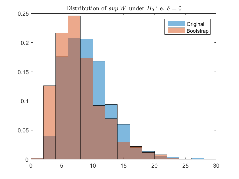
Figure 1: Original and bootstrapped $sup\textit{-}Wald$ statistics under $\mathcal{H}_{0}$

4.2 Test power

Here we tested three sets of coefficient choices, maintaining $\mathcal{H}_{1}:\delta\neq 0$ holds.

Parameters	Values	Rejection Probability
	(0.5, 0.8, 0.0, -0.5, 0.0)	1.00
$(\beta_{1},\beta_{2},\delta_{0},\delta_{1},\delta_{2})$	(0.5, 0.0, 0.0, -0.5, 0.0)	0.54
	(0.5, 0.0, 0.0, -0.9, 0.0)	0.96

We observe that our test has significant power to reject $\mathcal{H}_{0}$ when $\mathcal{H}_{1}$ is true, especially when the true $\delta$ is sufficiently far from zero.

5 Application

We apply our method to evaluate the effect of obesity on worker’s productivity. Obesity is measured with Body Mass Index (BMI), weight in kilograms divided by height in meters squared. Individuals whose BMI between 25 and 30 are considered to be overweight, and BMI of 30 or higher are treated as obese. Using data from the British Cohort Study and the methods described in the earlier section, we examine how BMI is associated with work hours. For more detailed discussion, see Kim (2019).

In this example, we consider work hours and BMI of male workers using the following model with a kink in BMI.

$$y_{it}=\beta_{0}+x_{it}\beta_{1}+q_{it}\beta_{2}+\delta(q_{it}-\gamma)1\{q_{it}\geq\gamma\}+\alpha_{i}+\varepsilon_{it},$$

where we present work hours as $y_{it}$ for an individual $i$ for a period $t,$ $x_{it}$ is family size and $q_{it}$ is BMI. We have two period panel data $(t=1,2)$ and take the first difference as follows to remove $\alpha_{i},$ the individual time-invariant charateristics that are associated with work hours.

$$\Delta y_{i2}=\Delta x_{i2}\beta_{1}+\Delta q_{i2}\beta_{2}+\delta(q_{i2}-\gamma)1\{q_{i2}\geq\gamma\}-(q_{i1}-\gamma)\delta 1\{q_{i1}\geq\gamma\}+\Delta\varepsilon_{i2}.$$

To implement GMM estimation, we use four instrumental variables, birth weight (bweight) and a worker’s own childhood BMI (bmic) and parents’ BMI (bmim, bmid), for BMI variables of $\Delta q_{i2},q_{i2},q_{i1}$ in the first differenced model.

After loading data, we first need to declare that the data is panel. The default model for xthenreg is a dynamic model. Since we consider a static model, not a dynamic model, we use static option. We also impose a kink in the model by using kink option.

. use hour, clear
. xtset ilabel time
. xthenreg hour bmi hsize, endo(bmi) inst(bweight $>$  bmic bmim bmid hsize) kink static

N = 768, T = 2
Panel Var. = ilabel
Time Var. = time
Number of moment conditions = 7

hour	Coef.	Std. Err.	z	P $>$$|$z$|$	[95% Conf.	Interval]
hsize_b	.4929009	.2707888	1.82	0.069	-.0378354	1.023637
bmi_b	-.7547926	.9564381	-0.79	0.430	-2.629377	1.119792
kink_slope	2.533467	2.170619	1.17	0.243	-1.720868	6.787802
r	29.04343	4.703686	6.17	0.000	19.82437	38.26248

The information preceding the table is as follows. N is the total number of unique subjects, T is the number of time periods. Number of moment conditions is provided based on the choice of instruments. In this example, we can obtain the same results by collecting all exogenous variables into one place with exo option as follows.

. xthenreg hour bmi, endo(bmi) exo(hsize) inst(bweight $>$  bmic bmim bmid) kink static

We can also change the set of included and excluded instruments using the inst option. The number of moment conditions varies accordingly.

. xthenreg hour bmi hsize, endo(bmi) inst(bweight $>$  bmic bmim bmid) kink static

N = 768, T = 2
Panel Var. = ilabel
Time Var. = time
Number of moment conditions = 6

hour	Coef.	Std.Err.	z	P $>$$|$z$|$	[95% Conf.	Interval]
hsize_b	.4964864	.2774487	1.79	0.074	-.0473031	1.040276
bmi_b	-.7783025	1.147452	-0.68	0.498	-3.027267	1.470662
kink_slope	2.527627	2.29367	1.10	0.270	-1.967884	7.023139
r	28.9816	6.002713	4.83	0.000	17.2165	40.7467

We can estimate the model with a restriction on the sample.

. xthenreg hour bmi if region==1, endo(bmi) exo(hsize) $>$   inst(bweight bmic bmim bmid) kink static

N = 637, T = 2
Panel Var. = ilabel
Time Var. = time
Number of moment conditions = 7

hour	Coef.	Std.Err.	z	P $>$$|$z$|$	[95% Conf.	Interval]
bmi_b	-.3205365	1.841899	-0.17	0.862	-3.930593	3.28952
hsize_b	.5270078	.3784874	1.39	0.164	-.2148138	1.268829
kink_slope	2.444602	7.610258	0.32	0.748	-12.47123	17.36043
r	29.14014	17.36101	1.68	0.093	-4.886813	63.16709

Next we consider discontinuity in BMI effect without imposing a kink in the model.

$$y_{it}=\beta_{0}+x_{it}\beta_{1}+q_{it}\beta_{2}+(\delta_{0}+x_{it}\delta_{1}+q_{it}\delta_{2})1\{q_{it}>\gamma\}+\alpha_{i}+\varepsilon_{it}.$$

By taking first difference, we obtain the following model and estimate it with only static option.

$$\Delta y_{i2}=\Delta x_{i2}\beta_{1}+\Delta q_{i2}\beta_{2}+(\delta_{0}+x_{i2}\delta_{1}+q_{i2}\delta_{2})1\{q_{i2}>\gamma\}-(\delta_{0}+x_{i1}\delta_{1}+q_{i1}\delta_{2})1\{q_{i1}>\gamma\}+\Delta\varepsilon_{i2}.$$

. xthenreg hour bmi, endo(bmi) exo(hsize) inst(bweight $>$   bmic bmim bmid) static

N = 768, T = 2
Panel Var. = ilabel
Time Var. = time
Number of moment conditions = 7

hour	Coef.	Std.Err.	z	P $>$$|$z$|$	[95% Conf.	Interval]
bmi_b	6.069513	19.04971	0.32	0.750	-31.26724	43.40626
hsize_b	-2.093733	16.48417	-0.13	0.899	-34.40211	30.21464
cons_d	106.3078	626.0473	0.17	0.865	-1120.722	1333.338
bmi_d	-5.569615	27.32028	-0.20	0.838	-59.11639	47.97716
hsize_d	4.898759	16.62541	0.29	0.768	-27.68644	37.48395
r	25.64312	14.89532	1.72	0.085	-3.551176	54.83741

References

• [1] Adam, C. S., and Bevan, D. L. (2005). “Fiscal deficits and growth in developing countries,” Journal of Public Economics, 89(4), 571-597.
• [2] Giacomini, R., Politis, D. N., & White, H. (2013). “A warp-speed method for conducting Monte Carlo experiments involving bootstrap estimators,” Econometric theory, 29(3), 567-589.
• [3] Hansen, B. E. (1999). “Threshold effects in non-dynamic panels: Estimation, testing, and inference,” Journal of econometrics, 93(2), 345-368.
• [4] Hidalgo, J., Lee, J., and M.H. Seo (2019). “Robust Inference for Threshold Regression Models,” Journal of Econometrics, to appear.
• [5] Khan, M. S., and Ssnhadji, A. S. (2001). “Threshold effects in the relationship between inflation and growth,” IMF Staff papers, 48(1), 1-21.
• [6] Kim, Y-J. (2019). “The effect of weight on work hours,” working paper.
• [7] Seo, M. and Y. Shin (2016). “Dynamic panels with threshold effect and endogeneity,” Journal of Econometrics, 195: 169-186.
• [8] Wang, Q. (2015). “Fixed-effect panel threshold model using Stata,” The Stata Journal, 15(1), 121-134.
• [9] Zhang, Y., Zhou, Q., and Jiang, L. (2017). “Panel kink regression with an unknown threshold,” Economics Letters, 157, 116-121.