Buy-many mechanisms are not much better than item pricing

Abstract

Multi-item mechanisms can be very complex offering many different bundles to the buyer that could even be randomized. Such complexity is thought to be necessary as the revenue gaps between randomized and deterministic mechanisms, or deterministic and simple mechanisms are huge even for additive valuations.

We challenge this conventional belief by showing that these large gaps can only happen in restricted situations. These are situations where the mechanism overcharges a buyer for a bundle while selling individual items at much lower prices. Arguably this is impractical in many settings because the buyer can break his order into smaller pieces paying a much lower price overall. Our main result is that if the buyer is allowed to purchase as many (randomized) bundles as he pleases, the revenue of any multi-item mechanism is at most $O(\log n)$ times the revenue achievable by item pricing, where $n$ is the number of items. This holds in the most general setting possible, with an arbitrarily correlated distribution of buyer types and arbitrary valuations.

We also show that this result is tight in a very strong sense. Any family of mechanisms of subexponential description complexity cannot achieve better than logarithmic approximation even against the best deterministic mechanism and even for additive valuations. In contrast, item pricing that has linear description complexity matches this bound against randomized mechanisms.

1 Introduction

It is well known that revenue optimal mechanisms can be complicated: when a seller has more than one item to sell to a buyer, the seller may price bundles of items rather than just the individual items; better still the seller may offer random subsets of items, also called lotteries; even more surprisingly, the seller may offer an infinitely large menu of such options. A primary line of enquiry within algorithmic mechanism design aims to establish simplicity versus optimality tradeoffs: is it possible to obtain some fraction of the optimal revenue via simple mechanisms, i.e. mechanisms that can be described easily, understood easily, and are prevalent in practice?

To quantify this tradeoff let us introduce some standard notation. Let Rev denote the optimal revenue obtained by using the most general kind of mechanism—a menu of lottery pricings. Let DRev denote the optimal revenue achieved by a deterministic mechanism—a menu of bundle pricings. Two “simple” mechanisms have been studied extensively in literature: item pricings, where each item is assigned a price and the buyer can buy any subset at the sum of the constituent prices; and bundle pricings, where every bundle is sold at a single constant price. The optimal revenues achievable by item pricings and bundle pricings are denoted SRev and BRev respectively. The goal then is to bound the ratios Rev/DRev, or ${\textsc{Rev}}/\max({\textsc{SRev}},{\textsc{BRev}})$, etc.

Briest et al. [6] were the first to show that revenue optimal mechanism design exhibits a particularly diabolical curse of dimensionality: whereas Rev/SRev is equal to 1 when the seller has only one item to sell, the ratio becomes infinite with three items even if the buyer is unit demand. Hart and Nisan [16] improved this to show that the ratio is infinite already with just two items. In fact, if the buyer has additive values over two items, meaning that the value of the bundle of two items is the sum over the individual item values, the ratio of Rev/DRev can also be infinite. Even focusing on just deterministic mechanisms, the situation is not much better: the ratio of DRev to SRev can be as large as $\Omega(2^{n}/n)$ with $n$ items and additive values. Daskalakis in his 2014 survey [12] summarized the situation as such: “Multi-item auctions defy intuition.”

Further work along these lines suggested that the existence of a good tradeoff depends on properties of the buyer’s valuation – both the structure of the value function as well as the distribution from which it is drawn. For example, two parallel lines of work investigating unit demand buyers [9, 11] and additive valuation buyers [15, 17, 1] respectively established that when the buyer’s values for different items are drawn independently, the larger of SRev and BRev is within a constant factor of Rev. These results extend to more general settings with subadditive valuations [19, 8] as well as multiple buyers [10, 21, 8, 7], but continue to require some degree of independence across individual item values.

Our work presents an alternate view of the simplicity versus optimality tradeoff. Our thesis is that the curse of dimensionality only happens when buyers’ actions are restricted. Let us illustrate through an example adapted from Hart and Nisan [16]. Consider a seller with $n$ items and a single buyer with additive values. Order all of the $2^{n}-1$ subsets of the items in weakly increasing order of size, and let $S_{i}$ denote the $i$th set in this ordering. The buyer’s value function is picked randomly from a set of $2^{n}-1$ different types. The $i$th type is realized with probability proportional to $n^{-i}$ and values every item in the set $S_{i}$ at $n^{i}/|S_{i}|$ and every item not in $S_{i}$ at $0$. It is now straightforward to see that a mechanism $\mathcal{M}$ that offers the set $S_{i}$ at a price of $n^{i-1}$ extracts as revenue a $1/n$ fraction of the buyer’s total expected value, or $\Omega(2^{n}/n)$—for every $i$, the type $i$ buyer extracts the most utility by purchasing the set $S_{i}$. On the other hand, the buyer’s expected value is distributed according to the equal revenue distribution, and so any bundle pricing extracts at most $O(1)$ revenue and any item pricing extracts at most $O(n)$. The implication is that optimal deterministic mechanisms can obtain exponentially larger revenue than simple ones.

We notice that $\mathcal{M}$ disallows buyer from purchasing more than one set of items offered by the seller. The single-buyer mechanism design problem is a convenient abstraction for settings with unlimited supply and multiple i. i. d. buyers. Upon finding a (near-)optimal mechanism for the single-buyer setting, we can apply the mechanism as-is in the latter setting, once for each buyer. However, in that context, mechanisms such as $\mathcal{M}$ offer buyers opportunities for arbitrage. Consider, in particular, a set $S_{i}$ of size $2$. $\mathcal{M}$ sells both of the items in $S_{i}$ individually at a price no more than a $1/n$ fraction of the price of $S_{i}$. A buyer of type $i$ can then participate in the mechanism twice, purchasing the constituents of $S_{i}$ individually and paying far less to the mechanism than before. In effect, $\mathcal{M}$ is not Sybil-proof.

Single-buyer mechanisms can without loss of generality be described as menus of options where each option is a random allocation (a.k.a. lottery) paired with a price. In this paper we study Sybil-proof or buy-many mechanisms where the buyer is allowed to purchase any multi-set of menu options (of arbitrary size). For deterministic menus, Sybil-proofness simply means that the prices assigned to different menu options are subadditive over subsets of items. As a corollary, item pricing and bundle pricing are already Sybil-proof. For general mechanisms, in fact, imposing the constraint of Sybil-proofness greatly limits the extent to which mechanisms can price discriminate between buyers of different types and, in particular, disallows the gap examples of Briest et al. and Hart and Nisan.

We can now again ask whether arbitrary, complicated Sybil-proof mechanisms can obtain unboundedly larger revenue (or, even exponentially or polynomially larger revenue, with respect to the dimension $n$) relative to simple mechanisms. Our main result is that they cannot:

Theorem 1.1.

For any arbitrary distribution over arbitrary valuation functions,

$$\frac{{\textsc{SybilProofRev}}}{{\textsc{SRev}}}=O(\log n).$$

Here SybilProofRev denotes the optimal revenue achievable through (potentially randomized) Sybil-proof mechanisms. Briest et al. [6] previously studied the gap between Sybil-proof mechanisms and item pricings for the special case of unit-demand buyers and proved the same upper bound. Our main contribution is to extend this result to arbitrary valuation functions and distributions over valuations. Indeed we make no assumptions whatsoever on the buyer’s valuations other than that they are monotone non-decreasing in the set of items allocated—allocating extra items to the buyer never lowers his value.

Can we do even better? We show that the above result is tight in a very strong sense:

Theorem 1.2.

There exists a distribution over additive values for which no mechanism with description complexity at most $2^{o(n^{1/6})}$ can obtain a $o(\log n)$ fraction of the optimal deterministic Sybil-proof revenue.

Observe that item pricings can be described using $O(n\log R)$ bits when values lie in the range $[1,R]$. We construct a distribution over additive values with $R<n$ and a deterministic subadditive pricing such that no mechanism that can be represented using $2^{o(n^{1/6})}$ bits can obtain a $o(\log n)$ fraction of the revenue of the subadditive pricing. We further show that for single-minded buyers, the gap cannot be improved in general even if the pricing we are comparing against is a submodular function. Briest et al. previously showed a similar result for unit-demand buyers, namely that the ratio $\frac{{\textsc{SybilProofRev}}}{{\textsc{SRev}}}$ can be $\Omega(\log n)$.

Menu size.

Our results also have implications for the menu size complexity of optimal auctions. The menu size of an auction, defined as the number of different outcomes the seller offers to the buyer, has been studied extensively in literature as a measure of complexity for single-buyer mechanisms (see, e.g., [16, 13, 2, 14]). One criticism of this notion of menu size is that some mechanisms can be described much more succinctly than indicated by their menu size, as is the case for item pricing. Hart and Nisan [16] introduced the alternate concept of “additive menu size”, namely the number of “basic” options a buy-many mechanism offers, and showed that even mechanisms with small additive menu size cannot capture a good fraction of the optimal revenue. Our results show that allowing the buyer to purchase multiple options doesn’t just allow a more succinct description of the mechanism, it also fundamentally changes the set of mechanisms available to the seller. In particular, buy-many mechanisms with even infinite additive menu size cannot capture any finite fraction of the overall optimal revenue Rev, as their revenue is bounded by SybilProofRev.

Our work calls for a new investigation of additive menu-size complexity of Sybil-proof mechanisms. A natural question, for example, is whether one can always obtain a constant fraction of the optimal Sybil-proof revenue via mechanisms with finite additive menu size. If so, what menu size is necessary to obtain a $1-\epsilon$ fraction of the optimal Sybil-proof revenue? Does it matter whether the buyer can select multiple options adaptively or non-adaptively? We leave these questions to future work.

Our techniques.

Henceforth we will represent single-buyer mechanisms as pricing functions that assign a price to every possible (random) allocation. For Sybil-proof mechanisms, this price corresponds to the cheapest manner in which the buyer can acquire a (collection of) lottery(ies) that dominates the desired random allocation. For a pricing function $p$ and value function $v$, let ${\textsc{Rev}}_{v}(p)$ denote the revenue the mechanism $p$ obtains from a buyer with value $v$. When $v$ is drawn from a distribution $\mathcal{D}$, the mechanism’s expected revenue is $\textrm{\bf E}_{v\sim\mathcal{D}}\!\left[{\textsc{Rev}}_{v}(p)\right]$. Our goal is to find for any given Sybil-proof pricing $p$ and distribution $\mathcal{D}$, a “simple” pricing $q$, such that $\textrm{\bf E}_{v\sim\mathcal{D}}\!\left[{\textsc{Rev}}_{v}(q)\right]$ is comparable to $\textrm{\bf E}_{v\sim\mathcal{D}}\!\left[{\textsc{Rev}}_{v}(p)\right]$.

As a first attempt towards this goal, we ask whether $p$ can be “point-wise” approximated by $q$. That is, does there exist a small $c>1$ such that for all random allocations $\lambda$, $q(\lambda)/c\leq p(\lambda)\leq q(\lambda)$? It turns out that for adaptively Sybil-proof pricings $p$, with $q$ being an additive function, taking $c=n$ suffices. Since our eventual goal is to obtain an approximation to revenue in expectation over a given value distribution, rather than point-wise over each possible lottery purchased, it is reasonable to expect that a scaling-type argument would provide an $O(\log c)$ approximation. In particular, let $\alpha$ be a random power of $2$ between $1/c$ and $1$, and let $\alpha q$ denote the pricing where every price in $q$ is scaled by the factor $\alpha$. Then it holds that for any $\lambda$, with probability $1/\log(c)$, $\alpha q(\lambda)$ is within $[1/2,1]$ times $p(\lambda)$. The implication is that a buyer purchasing $\lambda$ under $p$ would still be interested in purchasing $\lambda$ at the cheaper price offered by $\alpha q$, while paying at least half of what he was paying under $p$. However, there is a fallacy in this argument: a buyer that purchases $\lambda$ under $p$ may switch to purchasing a much cheaper allocation when offered the pricing $\alpha q$. Our main technical contribution is in dealing with the buyer’s incentives to argue that even if the buyer switches allocations, the resulting revenue is still significant large.

Formally we prove the following theorem, that may be of independent interest. The theorem states that if a pricing function $q$ point-wise $c$-approximates a pricing function $p$, then a particular (random) scaling of $q$ obtains an $O(\log c)$-approximation in revenue to $p$ with respect to any arbitrary distribution over valuation functions.

Theorem 1.3.

For any $c>1$, let $p$ and $q$ be any two pricing functions satisfying $q(\lambda)/c\leq p(\lambda)\leq q(\lambda)$ for all random allocations $\lambda\in\Delta(2^{[n]})$. Then there exists a distribution over “scaling factors” $\alpha\in[1/2c,1]$ such that for any valuation function $v$, $\operatorname{E}_{\alpha}[{\textsc{Rev}}_{v}(\alpha q)]\geq\frac{1}{2\log(2c)}{\textsc{Rev}}_{v}(p)$.

Theorem 1.3 shows that approximating a pricing function pointwise suffices to obtain a good approximation to the revenue.

Our lower bounds are obtained by considering a weaker notion of approximation of a pricing function $p$ using another function $q$ that exactly captures the revenue tradeoff over many natural valuation classes. It only requires the approximation be accurate in expectation over the “demand distribution”, i.e. the distribution over sets that are bought when the function $p$ is offered as a price menu to the buyer. We say that a pricing function $q$, $c$-approximates from below the pricing function $p$ over the demand distribution $\Pi$ if,

$$\textrm{\bf E}_{S\sim\Pi}\!\left[q(S)\mathbbm{1}_{q(S)\leq p(S)}\right]\geq\frac{1}{c}\textrm{\bf E}_{S\sim\Pi}\!\left[p(S)\right]$$ (1)

Note that the expectation in the right hand side of (1) is exactly the revenue of $p$, while the expectation in the left hand side is a proxy for the revenue of $q$. It assumes that the demand distribution over sets remains the same but a set is bought only if its price under $q$ is not higher than its price under $p$.

In fact, there is a distribution over single-minded buyers for which the expected revenues of $p$ and $q$ are exactly equal to the expressions above: we pick a set $S$ from the distribution $\Pi$ and assign a value of $p(S)$ to every superset of $S$, including itself, and a value of $0$ everywhere else.

Our lower bounds show that under this weaker notion of approximation, functions $q$ with subexponential description complexity cannot obtain better than $O(\log n)$ approximation, even for submodular pricing functions $p$. This directly implies that no simple mechanism can get better than logarithmic approximation to the optimal revenue for single minded-buyers (Theorem 4.1) and also extends to the case of additive buyers (Theorem 4.4).

While in general better-than-logarithmic approximation with simple mechanisms is not possible even for simple valuations, in Appendix B we offer improved upper bounds in special cases where the demand distribution has additional structure.

2 Notation and definitions

We study the following single-buyer mechanism design problem. A seller has $n$ heterogeneous items to sell to a single buyer. The buyer’s type is given by a valuation function $v$ that assigns non-negative values to every set of items: $v:2^{[n]}\to\mathcal{R}_{0}^{+}$. Values are monotone, meaning that for any $S$ and $T$ with $S\subset T\subseteq[n]$, $v(S)\leq v(T)$. The buyer’s type is drawn from an arbitrary known distribution $\mathcal{D}$ over the set of all possible valuation functions.

Any selling mechanism can be described as a menu of options, each of which assigns a price to a random allocation or lottery. Let $\Delta=\Delta(2^{[n]})$ denote the set of all probability distributions over sets of items and $\lambda\in\Delta$ denote a “lottery” or random allocation. We describe a mechanism using a pricing function $p:\Delta\to\mathcal{R}_{0}^{+}$; The price assigned to a lottery $\lambda\in\Delta$ is then given by $p(\lambda)$.

If a buyer with valuation $v$ buys a lottery $\lambda\in\Delta$ at price $p(\lambda)$, her utility from the purchase is given by

$$u(v,p,\lambda):=\textrm{\bf E}_{S\sim\lambda}\!\left[v(S)\right]-p(\lambda).$$

If a buyer with valuation $v$ purchases a multiset $\Lambda=\{\lambda_{1},\lambda_{2},\cdots,\lambda_{k}\}$ of lotteries with price function $p$, her utility from the purchase is given by

$$u(v,p,\Lambda):=\textrm{\bf E}_{S_{i}\sim\lambda_{i}\forall i\in{[k]}}\!\left[v\left(\bigcup_{i}S_{i}\right)\right]-\sum_{i\in[k]}p(\lambda_{i}).$$

We sometimes use $v(\lambda)$ as shorthand for $\textrm{\bf E}_{S\sim\lambda}\!\left[v(S)\right]$ and $v(\Lambda)$ likewise for the value assigned to the union of sets drawn from a multiset $\Lambda$ of lotteries.

Sybil-proofness and optimal revenue.

We say that a lottery $\lambda$ dominates another lottery (or a multiset of lotteries) $\lambda^{\prime}$ if there exists a coupling between a random draw $S$ from $\lambda$ and a random draw (or union of draws) $S^{\prime}$ from $\lambda^{\prime}$ such that $S$ is a superset of $S^{\prime}$. We are now ready to define Sybil-proofness.

Definition 2.1.

A mechanism or pricing $p:\Delta\to\mathcal{R}_{0}^{+}$ is Sybil-proof if for every multiset $\Lambda$ of lotteries there exists a single lottery $\lambda$ dominating it that is no more expensive: $p(\lambda)\leq\sum_{\lambda^{\prime}\in\Lambda}p(\lambda^{\prime})$.

Observe that if a lottery $\lambda$ dominates another lottery (or a multiset of lotteries) $\lambda^{\prime}$, then any buyer with a monotone valuation function obtains higher expected value from $\lambda$ than from $\lambda^{\prime}$. We therefore get the following observation:

Fact 2.1.

Given any Sybil-proof pricing $p$, for any buyer type $v$ it is optimal for the buyer to purchase a single lottery $\lambda=\operatorname{arg\,max}_{\lambda\in\Delta}(v(\lambda)-p(\lambda))$.

Given a Sybil-proof pricing $p$, we use $\lambda_{p}(v):=\operatorname{arg\,max}_{\lambda\in\Delta}(v(\lambda)-p(\lambda))$ to denote the lottery purchased by a buyer with value function $v$, and $u(v,p)$ as the corresponding utility achieved. For convenience, we overload notation and use $p(v):=p(\lambda_{p}(v))$ to denote the price paid by the buyer. Given a distribution $\mathcal{D}$ over buyer types, we write ${\textsc{Rev}}_{\mathcal{D}}(p):=\textrm{\bf E}_{v\sim\mathcal{D}}\!\left[p(v)\right]$ as the revenue of the pricing $p$. The optimal Sybil-proof revenue for distribution $\mathcal{D}$ is given as follows; we drop the subscript $\mathcal{D}$ when it is clear from the context.

$${\textsc{SybilProofRev}}_{\mathcal{D}}:=\max_{\text{Sybil-proof pricings }p}{\textsc{Rev}}_{\mathcal{D}}(p).$$

Adaptive Sybil-proofness.

Our definition of Sybil-proofness guards against buyers that purchase multiple options from the given menu and receive a random allocation for each. The buyer can perform even better if these menu options are selected sequentially and adaptively—that is, if the buyer observes the instantiation of each random allocation before deciding whether and what to purchase next. Guarding against such an adaptive buyer places a further restriction on the prices the mechanism can charge. Let $\mathcal{A}$ denote a buying strategy, that is, an adaptive sequence of lotteries. Let $\Lambda_{\mathcal{A}}$ denote the (random) sequence of lotteries bought in $\mathcal{A}$. As before, we say that $\mathcal{A}$ is dominated by a lottery $\lambda$ if there exists a coupling between a random draw $S$ from $\lambda$ and a random union of draws $S^{\prime}$ from $\Lambda_{\mathcal{A}}$ such that $S$ is a superset of $S^{\prime}$. We can now define a more restrictive definition of Sybil-proofness:

Definition 2.2.

A mechanism or pricing $p:\Delta\to\mathcal{R}_{0}^{+}$ is Adaptively Sybil-proof if for every adaptive buying strategy $\mathcal{A}$ there exists a single lottery $\lambda$ dominating it that is cheaper: $p(\lambda)\leq\textrm{\bf E}_{\Lambda_{\mathcal{A}}}\!\left[\sum_{\lambda^{\prime}\in\Lambda_{\mathcal{A}}}p(\lambda^{\prime})\right]$.

Of course there is no way for the seller to enforce whether buyers can make purchasing decisions adaptively or non-adaptively, so it is natural to study mechanisms satisfying adaptive Sybil-proofness. Competing against optimal adaptively Sybil-proof mechanisms makes some of our arguments easier. However, all of our positive results also apply to the less restrictive notion of (non-adaptive) Sybil-proofness.

Deterministic mechanisms.

Deterministic mechanisms price only deterministic sets (a.k.a. bundles) of items—$p:2^{[n]}\to\mathcal{R}_{0}^{+}$. A deterministic pricing $p$ is Sybil-proof if and only if it is monotone and subadditive, that is, for any $S_{1}\subset S_{2}\subseteq[n]$, $p(S_{1})\leq p(S_{2})$, and for any set of bundles, $\mathcal{T}\subseteq 2^{[n]}$, the prices of the union of bundles is no more than the sum of individual bundle prices: $\sum_{S\in\mathcal{T}}p(S)\geq p(\cup_{S\in\mathcal{T}}\,S)$. The optimal deterministic Sybil-proof revenue for distribution $\mathcal{D}$ is given as follows.

$${\textsc{DetSybilProofRev}}_{\mathcal{D}}:=\max_{\begin{subarray}{c}\text{Deterministic monotone}\\ \text{subadditive pricings }p\end{subarray}}{\textsc{Rev}}_{\mathcal{D}}(p).$$

Simple pricings.

An item pricing is a deterministic additive pricing: $p(S)=\sum_{i\in S}p(\{i\})$ for all $S\subseteq[n]$. A bundle pricing is a constant pricing that assigns the same price to every set: $p(S)=p([n])$ for all $S\subseteq[n]$. Observe that item pricings and bundle pricings are always Sybil-proof. We use SRev and BRev to denote the optimal revenue achievable using item pricings and bundle pricings respectively (over an implicit distribution $\mathcal{D}$).

3 Approximation via item pricing

In this section we present our main upper bound, namely that the ratio between ${\textsc{SybilProofRev}}_{\mathcal{D}}$ and ${\textsc{SRev}}_{\mathcal{D}}$ is bounded by $O(\log n)$ for any value distribution $\mathcal{D}$. This result is based on ideas that are present implicitly in the work of Briest et al. [6] for unit-demand buyers. We formalize and extend these ideas to arbitrary valuations.

Our argument proceeds in two parts. First, we show that in order to approximate the expected revenue of a pricing $p$ with a pricing $q$ within some factor $\beta$, it suffices to obtain a point-wise $2^{O(\beta)}$-approximation of $p$ via $q$. Then we show that adaptively Sybil-proof pricings $p$ can be point-wise $n$-approximated by additive pricings. This provides a bound on the gap between adaptive ${\textsc{SybilProofRev}}_{\mathcal{D}}$ and ${\textsc{SRev}}_{\mathcal{D}}$. In the last part of this section, we extend our result to non-adaptively Sybil-proof pricings.

3.1 Point-wise approximation implies revenue approximation

Suppose that we have two pricing functions $p$ and $q$ that are close on every possible (random) allocation. In particular, for some $c>1$, we have $q(\lambda)/c\leq p(\lambda)\leq q(\lambda)$ for every random allocation $\lambda\in\Delta$. We say that $q$ point-wise $c$-approximates $p$. We will now prove Theorem 1.3, namely that a point-wise $c$-approximation implies an $O(\log c)$-approximation in revenue.

Theorem 1.3.

For any $c>1$, let $p$ and $q$ be any two pricing functions satisfying $q(\lambda)/c\leq p(\lambda)\leq q(\lambda)$ for all random allocations $\lambda\in\Delta(2^{[n]})$. Then there exists a distribution over “scaling factors” $\alpha\in[1/2c,1]$ such that for any valuation function $v$, $\operatorname{E}_{\alpha}[{\textsc{Rev}}_{v}(\alpha q)]\geq\frac{1}{2\log(2c)}{\textsc{Rev}}_{v}(p)$.

Our argument considers a suite of pricings $\{\alpha q\}$ defined over a range of scale factors $\alpha\in[1/2c,1]$. We want to argue that this suite of pricings collectively obtains good revenue from every buyer type. At the heart of our argument is the following observation: for any buyer type, if the buyer obtains much larger utility at low prices ($\frac{1}{2c}q$) than at high prices ($q$), we can capture a good fraction of this difference in utilities as revenue by picking a scaling factor $\alpha$ from an appropriate distribution independent of the buyer’s type. We formalize this observation as Lemma 3.1 below. We then argue that if $q$ point-wise approximates $p$, then this difference of utilities is proportional to the revenue obtained by $p$ from the buyer.

Lemma 3.1.

For any pricing $q$ and any $0<\ell\leq h$, let $\alpha$ be drawn from $[\ell,h]$ with density function $\frac{1}{\alpha\log(h/\ell)}$. Then, for any valuation function $v$,

$$\operatorname{E}_{\alpha}[{\textsc{Rev}}_{v}(\alpha q)]\geq\frac{u(v,\ell q)-u(v,hq)}{\log(h/\ell)}.$$

To understand the lemma, consider starting at $\alpha=\ell$ and gradually increasing the scaling factor and, correspondingly, prices. As the prices increases, the buyer’s utility from purchasing his favorite bundle weakly decreases. As long as the buyer continues to buy the same lottery, this decrease in utility is captured as revenue. At certain price points the buyer switches to buying a different lottery, causing the revenue to drop discontinuously. Other than these discontinuities, however, the buyer’s loss in utility is captured exactly as increase in revenue (see Figure 1). This observation allows us to relate the gradient of the revenue as a function of the scaling factor $\alpha$ to the gradient of the utility. Our next observation is that because revenue depends linearly on the scaling factor $\alpha$ (except at the break points), the revenue is proportional to its gradient. Then by picking an appropriate distribution on $\alpha$, we can capture exactly this gradient as expected revenue. We now present this argument formally.

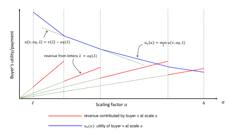
Figure 1: Utility and revenue as function of the scaling factor $\alpha$. Our goal is to find a distribution on $\alpha$ such that the expected revenue (red curve) is proportional to the change in utility (blue curve).

Proof.

Consider a buyer with value function $v$. Let ${u_{v}}(\alpha)$ denote the utility the buyer derives when offered the pricing $\alpha q$, and $\lambda_{\alpha}$ denote the corresponding lottery purchased:

$${u_{v}}(\alpha) =\max_{\lambda\in\Delta}\,(v(\lambda)-\alpha q(\lambda))$$

$$\lambda_{\alpha} =\operatorname{arg\,max}_{\lambda\in\Delta}\,(v(\lambda)-\alpha q(\lambda)).$$

By the envelope theorem it holds that ${u_{v}}^{\prime}(\alpha)=\frac{\textrm{d}}{\textrm{d}\alpha}(v(\lambda_{\alpha})-\alpha q(\lambda_{\alpha}))=-q(\lambda_{\alpha})$. Therefore, the seller’s revenue from this buyer is given by

$$\alpha q(\lambda_{\alpha})=-\alpha{u_{v}}^{\prime}(\alpha).$$

Now, consider picking $\alpha$ from the equal revenue distribution over $[\ell,h]$ with density function $1/(\alpha\log(h/\ell))$, and offering the buyer the pricing $\alpha q$. Then, the expected revenue from this buyer is:

$$\int_{\ell}^{h}\alpha q(\lambda_{\alpha})\cdot\frac{1}{\alpha\log(h/\ell)}d\alpha =\frac{-1}{\log(h/\ell)}\int_{\ell}^{h}{u_{v}}^{\prime}(\alpha)d\alpha=\frac{{u_{v}}(\ell)-{u_{v}}(h)}{\log(h/\ell)}.$$

∎

We are now ready to complete the proof of Theorem 1.3.

Proof of Theorem 1.3. Fix a buyer valuation $v$, and let $h=1$ and $\ell=1/2c$. We will bound the utility the buyer derives under pricings $\ell q$ and $hq$ in terms of his utility under $p$.

$$u(v,\ell q)=\max_{\lambda\in\Delta}\left(v(\lambda)-\frac{1}{2c}q(\lambda)\right)\geq\max_{\lambda\in\Delta}\left(v(\lambda)-\frac{1}{2}p(\lambda)\right)\geq u(v,p)+\frac{1}{2}p(v).$$

On the other hand,

$$u(v,hq)=\max_{\lambda\in\Delta}\left(v(\lambda)-q(\lambda)\right)\leq\max_{\lambda\in\Delta}\left(v(\lambda)-p(\lambda)\right)=u(v,p).$$

We can now apply Lemma 3.1 to obtain a revenue of at least $\frac{1}{2\log(2c)}p(v)$ from the buyer. ∎

3.2 Upper bound for adaptively Sybil-proof pricings

As a warm-up to our main theorem, we show how Theorem 1.3 can be directly applied to get an upper bound on ${\textsc{SybilProofRev}}_{\mathcal{D}}/{\textsc{SRev}}_{\mathcal{D}}$ for adaptively Sybil-proof pricings. We first briefly sketch the proof for deterministic Sybil-proof pricings. Recall that deterministic Sybil-proof pricings are monotone subadditive functions. Let $p$ be any such pricing. Then, by defining $q$ to be identical to $p$ over singletons ($q(\{i\})=p(\{i\})$ for all $i\in[n]$) and extending it additively to bundles ($q(S)=\sum_{i\in S}q(\{i\})$), we observe on the one hand that $q$ is no smaller than $p$ on any set $S$. On the other hand, $p(S)$ is at least as large as the price of the most expensive singleton item in $S$, which is at least as large as the average price of an item in $S$, or $q(S)/n$. Therefore, $q$ point-wise $n$-approximates $p$. We can therefore apply Theorem 1.3 to obtain an $O(\log n)$ approximation to the expected revenue of $p$ under any value distribution. We now formalize this argument for randomized adaptively Sybil-proof pricings.

Theorem 3.2.

For any distribution $\mathcal{D}$, we have ${\textsc{AdaptSybilProofRev}}_{\mathcal{D}}\leq O(\log n){\textsc{SRev}}_{\mathcal{D}}$.

Proof.

Let $p$ be the adaptive Sybil-proof pricing that achieves revenue ${\textsc{AdaptSybilProofRev}}_{\mathcal{D}}$. We again begin by defining base prices for each of the items. Informally, these are the minimum prices the buyer needs to pay in expectation to obtain item $i$ with certainty:

$$q(\{i\})=\min_{\lambda\in\Delta}\,\frac{p(\lambda)}{\Pr[i\in\lambda]}$$

where we write $\Pr[i\in\lambda]$ as shorthand for $\Pr_{S\sim\lambda}[i\in S]$. Let $\lambda_{i}$ denote the lottery that defines the price for item $i$: $\lambda_{i}=\operatorname{arg\,min}_{\lambda\in\Delta}\,\frac{p(\lambda)}{\Pr[i\in\lambda]}$. For every $\lambda\in\Delta$, $q(\lambda)=\sum_{S\subseteq[n]}\lambda(S)\sum_{i\in S}q(\{i\})$.

Observe that for any lottery $\lambda\in\Delta$, the adaptive buyer can draw a set $T$ from $\lambda$ and purchase this set by purchasing for every $i\in T$ the lottery $\lambda_{i}$ repeatedly until he obtains the item. The expected price paid by the buyer in this strategy is precisely $\textrm{\bf E}_{T\sim\lambda}\!\left[q(T)\right]=\sum_{i\in[n]}(q(\{i\})\Pr[i\in\lambda])=q(\lambda)$. Since $p$ is adaptively Sybil-proof, we have $p(\lambda)\leq q(\lambda)$.

On the other hand, by the definition of $q$, $p(\lambda)\geq q(\{i\})\Pr[i\in\lambda]$ and therefore, summing over all $i\in[n]$ and dividing by $n$, we have $p(\lambda)\geq\frac{1}{n}q(\lambda)$. Taking $c=n$ in Theorem 1.3 finishes the proof. ∎

3.3 Upper bound for general randomized Sybil-proof pricings

We will now prove our main theorem:

Theorem 1.1.

For any arbitrary distribution over arbitrary valuation functions,

$$\frac{{\textsc{SybilProofRev}}}{{\textsc{SRev}}}=O(\log n).$$

As in our argument for the adaptive setting, consider any Sybil-proof pricing $p$ and let us define the pricing $q$ as:

$$q(\{i\})=\min_{\lambda\in\Delta}\,\frac{p(\lambda)}{\Pr[i\in\lambda]}\,\,\forall i\in[n]\qquad\text{ and }\qquad q(S)=\sum_{i\in S}q(\{i\})\,\,\forall S\subseteq[n].$$

Our goal, as before, is to argue that $q$ point-wise approximates $p$. It is straightforward to argue that $p(\lambda)\geq\frac{1}{n}q(\lambda)$ for all $\lambda\in\Delta$. However, it is no longer necessarily true that $p(S)\leq q(S)$ for all sets $S$ of items. This is because acquiring the set $S$ non-adaptively with certainty under $p$ may cost much more than $q(S)$. This in turn implies that the buyer’s utility under $q$ may be larger than his utility under $p$. Indeed no matter how large of a scaling factor $h$ we pick, it is tricky to directly argue that $u(v,hq)\leq u(v,p)$. Instead, we will argue that if the set $S$ the buyer wants to purchase under $hq$ is too expensive to purchase under $p$, this happens because some high value item in $S$ can only be bought with very low probability in $p$. We will use such items as the basis to construct a different additive pricing that obtains a good fraction of the revenue of $p$. We now formalize this argument.

Proof.

Let $p$ be the Sybil-proof pricing that achieves revenue ${\textsc{SybilProofRev}}_{\mathcal{D}}$. Let $\ell=1/2n$, $h=4n$, and define the pricing $q$ as above. Let $\alpha$ be picked from the range $[\ell,h]$ with density function $1/(\alpha\log(h/\ell))$. Then for any valuation function $v$, it is straightforward to observe that $u(v,\ell q)\geq u(v,p)+p(v)/2$. We will now focus on bounding $u(v,hq)$.

Let $T_{h}$ be the set purchased by the buyer when offered the pricing $hq$. Then $u(v,hq)=v(T_{h})-hq(T_{h})$. We want to bound this utility in terms of the utility the buyer gets under the pricing $p$, so let us consider how much it would cost the buyer to acquire $T_{h}$ under $p$. In particular, fix some number $m$ and suppose that the buyer purchases a multiset $\Lambda_{m}$ that contains $m_{i}=\lceil\frac{m}{\Pr[i\in\lambda_{i}]}\rceil$ copies of $\lambda_{i}$ for all $i\in T_{h}$. Then, the probability that some $i\in T_{h}$ does not belong to the random allocation drawn from this multiset is at most $(1-\Pr[i\in\lambda_{i}])^{m_{i}}<2^{-m}$. Accordingly, the probability that $T_{h}$ is not a subset of the random allocation drawn from $\Lambda_{m}$ is at most $n2^{-m}$. The total price of $\Lambda_{m}$ is $\sum_{i\in T_{h}}\lceil\frac{m}{\Pr[i\in\lambda_{i}]}\rceil\,p(\lambda_{i})\leq(m+1)\sum_{i\in T_{h}}q(\{i\})=(m+1)q(T_{h})$. We therefore have:

$$u(v,p)\geq u(v,p,\Lambda_{m})\geq(1-n2^{-m})v(T_{h})-(m+1)q(T_{h})\quad\text{for all }m.$$

Now, let $k$ be defined such that $n2^{-k}v(T_{h})=q(T_{h})$, that is, $k=\log(nv(T_{h})/q(T_{h}))$. Then we get:

$$u(v,p) \geq v(T_{h})-(k+2)q(T_{h})$$ and,

$$u(v,hq) \leq u(v,p)+(k+2-h)q(T_{h}).$$ (2)

Now, if $k+2\leq h$, then we already have the bound we desire. So, for the remainder of the proof, assume that $k>h-2\geq 3n$. We will construct a different item pricing to recover the quantity $(k+2-h)q(T_{h})<kq(T_{h})$ as revenue from the buyer with value $v$.

For any $T\subseteq[n]$ and positive integer $a$, the (uniform) item pricing $\tilde{g}_{T,a}$ is defined as follows: $\tilde{g}_{T,a}(S)=2^{a+n}q(T)|S|$ for all $S\subseteq[n]$. Now consider a buyer with value function $v$ and with $k=\log(nv(T_{h})/q(T_{h}))$. When offered the pricing $\tilde{g}_{T_{h},a}$ with $a<k-n-2\log n$, this buyer obtains a utility of at least $v(T_{h})-\tilde{g}_{T_{h},a}(T_{h})\geq v(T_{h})-2^{a+n}nq(T_{h})>v(T_{h})-\frac{1}{n}2^{k}q(T_{h})=0$. Therefore, the buyer buys at least one item under this pricing and pays at least $2^{a+n}q(T_{h})$. In other words,

$$\tilde{g}_{T_{h},a}(v)\geq 2^{a+n}q(T_{h})\quad\text{for }a<k-n-2\log n.$$

Let $T$ be drawn from the uniform distribution over $2^{[n]}$ and $a$ be drawn from the geometric distribution with mean 2, that is, $\Pr[a=x]=2^{-x-1}$ for every $x\in\mathbb{N}$. Then, we get:

$$\textrm{\bf E}_{T,a}\!\left[{\textsc{Rev}}_{v}(\tilde{g}_{T,a})\right] \geq\frac{1}{2^{n}}\sum_{a=0}^{k-n-2\log n-1}\frac{1}{2^{a+1}}2^{a+n}q(T_{h})$$

$$=\frac{1}{2}(k-n-2\log n-1)q(T_{h})$$

$$\geq\frac{1}{4}kq(T_{h})\quad\text{for }k\geq h-2.$$ (3)

Finally we apply Lemma 3.1 with $h=4n$ and $\ell=1/2n$:

$$\log(8n^{2})\textrm{\bf E}_{\alpha}\!\left[\alpha q(v)\right] =u(v,\ell q)-u(v,hq)=u(v,p)-u(v,hq)+\frac{1}{2}p(v)$$ (4)

Putting together Equations (2), (3), and (4), we get that for any buyer valuation $v$:

$$\log(8n^{2})\textrm{\bf E}_{\alpha}\!\left[{\textsc{Rev}}_{v}(\alpha q)\right]+4\textrm{\bf E}_{T,a}\!\left[{\textsc{Rev}}_{v}(\tilde{g}_{T,a})\right] \geq\frac{1}{2}p(v).$$

The theorem now follows by taking expectations over the valuation function $v$ and recalling that $\{\alpha q\}$ and $\{\tilde{g}_{T,a}\}$ are all additive pricing functions.

∎

4 Lower Bound

In this section we present our main lower bound, namely that the $O(\log n)$ approximation achieved in the previous section is tight in a very strong sense. We show that there exists a distribution over additive buyer types such that no mechanism with sub-exponential description complexity can $o(\log n)$-approximate the revenue from optimal deterministic Sybil-proof pricing. This implies in particular that no simple mechanism can achieve better than logarithmic approximation, including popular mechanisms studied in previous work such as selling separately, selling the grand-bundle, partition mechanisms or any combination of these mechanisms.

Before presenting our results for additive buyers, we first consider the simpler case where buyers are single-minded, i.e. they are only interested in purchasing a single set.

Our construction proceeds by identifying a large class of subadditive functions that assign independently arbitrary values in $[n^{1/6},n^{1/3}]$ to exponentially many sets $S_{1},S_{2},\cdots,S_{N}$. For any function $p$ in this class, pricing according to $p$ extracts full surplus from a distribution over single minded buyers where a buyer wanting set $S_{i}$ has value $p(S_{i})$. Getting an $O(\log n)$ approximation for such a distribution as in the previous section is easy by setting the same price for every subset since there are only $O(\log n)$ different scales of prices to choose from. However, to obtain a better approximation one would need to charge high or low prices at different sets which requires at least one bit per set to describe. As there are exponentially many sets, mechanisms with subexponential description complexity cannot obtain better than logarithmic approximation.

4.1 The basic construction and a lower bound for single-minded buyers

Let $p$ and $q$ be any two functions defined over the subsets of $[n]$. Let ${\Pi}$ be a demand distribution over sets, ${\Pi}\in\Delta(2^{[n]})$. We will say that $q$ $c$-approximates $p$ from below over ${\Pi}$ if the following holds:

$$\textrm{\bf E}_{S\sim{\Pi}}\!\left[q(S)\mathbbm{1}_{q(S)\leq p(S)}\right]\geq\frac{1}{c}\textrm{\bf E}_{S\sim{\Pi}}\!\left[p(S)\right].$$

Our argument will proceed in two parts. First, we will show that for any “small” class of functions $q$, there exists a subadditive (in fact, submodular) $p$ and a distribution ${\Pi}$ such that no $q$ in the class can $o(\log n)$-approximate $p$ from below over ${\Pi}$. Then we will show that for any $p$ and ${\Pi}$ of the form constructed in the first step, there exists a distribution over valuation functions such that the optimal subadditive revenue is a constant fraction of $\textrm{\bf E}_{S\sim{\Pi}}\!\left[p(S)\right]$, while the revenue of any other function $q$ is exactly $\textrm{\bf E}_{S\sim{\Pi}}\!\left[q(S)\mathbbm{1}_{q(S)\leq p(S)}\right]$ for single-minded buyers. Together this will imply the following theorem.

Theorem 4.1.

For any large enough $n$, there exists a distribution $\mathcal{D}$ over single-minded valuation functions over $n$ items and a deterministic submodular pricing function $p$ such that ${\textsc{Rev}}_{\mathcal{D}}(p)$ is a factor of $\Omega(\log n)$ larger than the revenue of any pricing that can be described using $2^{o(n^{1/6})}$ bits.

Let us begin by describing the class of subadditive functions $p$ that we will use in our argument. Let $\mathcal{S}=\{S_{1},S_{2},\cdots,S_{N}\}$ be a collection of $N$ subsets of $[n]$. Let $\beta=(b_{1},\cdots,b_{N})$ be a vector of integers of size $N$, where each coordinate is picked from the range $[b_{\min},b_{\max}]$. We define a partial function ${p_{\mathcal{S},\beta}}$ as follows: for all $S_{i}\in\mathcal{S}$, set ${p_{\mathcal{S},\beta}}(S_{i})=b_{i}$. The following lemma follows from the work of Balcan and Harvey [4] and shows that we can pick both $N$ and $b_{\max}/b_{\min}$ to be sufficiently large while ensuring that $p$ is submodular. See the appendix for a proof.

Lemma 4.2.

Let $N=2^{n^{1/6}/8}$, $b_{\min}=n^{1/6}$, and $b_{\max}=n^{1/3}$. Then, there exists a collection of sets $\mathcal{S}=\{S_{1},S_{2},\cdots,S_{N}\}$, such that for each $i$ $|S_{i}|=n^{1/3}$; for each $i\neq j$, $|S_{i}\cap S_{j}|\leq n^{1/6}$; and for any integral vector $\beta\in[b_{\min},b_{\max}]^{N}$, the partial function ${p_{\mathcal{S},\beta}}$ can be completed to a matroid rank function.

Let ${\Pi}$ be the uniform distribution over the collection $\mathcal{S}$. Our next lemma argues that for any small class of functions $\mathcal{Q}$, there exists a vector $\beta$, such that no function in $\mathcal{Q}$ can $c$-approximate ${p_{\mathcal{S},\beta}}$ from below over ${\Pi}$. Observe that because ${\Pi}$ only places non-zero mass over sets in $\mathcal{S}$, we do not need to specify a completion of ${p_{\mathcal{S},\beta}}$ for this lemma.

Lemma 4.3.

Let $m=\log(b_{\max}/b_{\min})$, $c\leq m/8$, and $\mathcal{Q}$ be an arbitrary class of functions defined over the subsets of $[n]$ with $|\mathcal{Q}|\leq 2^{o(N/4^{m})}$. Then there exists an integral vector $\beta\in[b_{\min},b_{\max}]^{N}$ such that no function $q\in\mathcal{Q}$ can $c$-approximate ${p_{\mathcal{S},\beta}}$ from below over ${\Pi}$.

Proof.

Fix a function $q\in\mathcal{Q}$. We will pick $\beta$ from a distribution and show that the probability that $q$ $c$-approximates the corresponding function ${p_{\mathcal{S},\beta}}$ is small. For each $i\in[N]$, draw $b_{i}$ independently according to the following truncated geometric distribution: $\Pr[b_{i}=2^{k}b_{\min}]=\frac{2^{-k}}{1-2^{-m}}$ for $1\leq k\leq m$. Let $h_{i}=q(S_{i})\mathbbm{1}_{q(S_{i})\leq{p_{\mathcal{S},\beta}}(S_{i})}$ be a random variable that depends on $\beta$. Then the statement that $q$ $c$-approximates ${p_{\mathcal{S},\beta}}$ from below over ${\Pi}$ is equivalent to the statement that

$$\sum_{i\in[N]}h_{i}\geq\frac{1}{c}\sum_{i\in[N]}{p_{\mathcal{S},\beta}}(S_{i}).$$ (5)

Observe that over the randomness in $\beta$, the variables $h_{i}$ are independent and bounded. For all $i$, $h_{i}\leq{p_{\mathcal{S},\beta}}(S_{i})\leq 2^{m}b_{\min}$. Furthermore,

$$\textrm{\bf E}\!\left[h_{i}\right]=q(S_{i})\Pr[{p_{\mathcal{S},\beta}}(S_{i})\geq q(S_{i})]\leq q(S_{i})\frac{2b_{\min}}{q(S_{i})}=2b_{\min}.$$

On the other hand,

$$\textrm{\bf E}\!\left[{p_{\mathcal{S},\beta}}(S_{i})\right]=\textrm{\bf E}\!\left[b_{i}\right]=\frac{m}{1-2^{-m}}b_{\min}.$$

We can now bound the probability that (5) holds by applying concentration to the sums of $h_{i}$ and ${p_{\mathcal{S},\beta}}(S_{i})$ respectively.

$$\Pr_{\beta}\left[\sum_{i}h_{i}\right. \geq \left.\frac{1}{c}\sum_{i}{p_{\mathcal{S},\beta}}(S_{i})\right]$$

$$\leq \Pr\left[\sum_{i}h_{i}\geq\frac{1}{2c}\textrm{\bf E}\!\left[\sum_{i}{p_{\mathcal{S},\beta}}(S_{i})\right]\right]+\Pr\left[\sum_{i}{p_{\mathcal{S},\beta}}(S_{i})<\frac{1}{2}\textrm{\bf E}\!\left[\sum_{i}{p_{\mathcal{S},\beta}}(S_{i})\right]\right]$$

$$= \Pr\left[\sum_{i}h_{i}\geq\frac{m}{2c(1-2^{-m})}Nb_{\min}\right]+\Pr\left[\sum_{i}{p_{\mathcal{S},\beta}}(S_{i})<\frac{m}{2(1-2^{-m})}Nb_{\min}\right]$$

$$\leq \exp\left(-\frac{2(\frac{m}{2c(1-2^{-m})}Nb_{\min}-2Nb_{\min})^{2}}{N(2^{m}b_{\min})^{2}}\right)+\exp\left(-\frac{2(\frac{m}{2(1-2^{-m})}Nb_{\min})^{2}}{N(2^{m}b_{\min})^{2}}\right)$$

$$= O(2^{-N4^{-m}}).$$

Here the third line uses Hoeffding’s inequality by observing that $0\leq h_{i},{p_{\mathcal{S},\beta}}(S_{i})\leq 2^{m}b_{\min}$; the last line follows using $c\leq m/8$. The lemma now follows by taking the union bound over all $q\in\mathcal{Q}$. ∎

We are now ready to prove Theorem 4.1.

Proof of Theorem 4.1. Let $b_{\min}$, $b_{\max}$, $N$, and $\mathcal{S}$ be as given in Lemma 4.2. Let ${\Pi}$ be the uniform distribution over $\mathcal{S}$. Let $m=\log(b_{\max}/b_{\min})$, $c=m/8=\Omega(\log n)$, and observe that the class $\mathcal{Q}$ of all pricings that can be described using $2^{o(n^{1/6})}$ bits has size $2^{o(N/4^{m})}$. So we can apply Lemma 4.3 to obtain a vector $\beta$.

Now we will define a distribution $\mathcal{D}$ over valuation functions as follows. For $i\in[N]$, let $v_{i}$ be the function that takes on value $b_{i}$ over any superset of $S_{i}$ and value $0$ otherwise. Function $v_{i}$ is instantiated with probability $1/N$. Let $p$ be the completion of ${p_{\mathcal{S},\beta}}$ as given by Lemma 4.2. Consider a pricing function that assigns a price of $\frac{1}{2}p(S)$ to any set $S\subseteq[n]$. Since this function is subadditive and a buyer with value $v_{i}$ is single-minded and can afford to buy the set $S_{i}$, the mechanism obtains a revenue of $\frac{1}{2}p(S_{i})$ from this buyer. The mechanism’s expected revenue over the distribution $\mathcal{D}$ is then $\frac{1}{2}\textrm{\bf E}_{S\sim{\Pi}}\!\left[{p_{\mathcal{S},\beta}}(S)\right]$.

On the other hand, for any monotone pricing function $q$, a buyer with value function $v_{i}$ purchases the set $S_{i}$ if and only if $q(S_{i})\leq v_{i}(S_{i})=b_{i}={p_{\mathcal{S},\beta}}(S_{i})$. Therefore, the revenue of such a function $q$ over $\mathcal{D}$ is at most $\textrm{\bf E}_{S\sim{\Pi}}\!\left[q(S)\mathbbm{1}_{q(S)\leq p(S)}\right]$.

The theorem now follows by applying Lemma 4.3. ∎

4.2 A lower bound for additive buyers

We now extend our lower bound to additive value buyers. Our construction is similar to that for Theorem 4.1 but there are some subtle differences. As before, let $\mathcal{S}=\{S_{1},S_{2},\cdots,S_{N}\}$ and $\beta=(b_{1},\cdots,b_{N})\in[b_{\min},b_{\max}]^{N}$. We now state and prove our lower bound for additive buyers.

Theorem 4.4.

For any large enough $n$, there exists a distribution $\mathcal{D}$ over additive valuation functions over $n$ items and a deterministic monotone subadditive pricing function $p$ such that ${\textsc{Rev}}_{\mathcal{D}}(p)$ is a factor of $\Omega(\log n)$ larger than the revenue of any mechanism that can be described using $2^{o(n^{1/6})}$ bits.

Proof.

Let $N$ and $\mathcal{S}$ be as defined in Lemma 4.2. Let $b_{\min}=2n^{1/6}$, $b_{\max}=n^{1/3}$, and fix an integral vector $\beta\in[b_{\min},b_{\max}]^{N}$. Consider the following distribution $\mathcal{D}_{\beta}$ over value functions. For $i\in[N]$, $v_{i,\beta}$ is an additive function that takes on the value $b_{i}/|S_{i}|$ over all items in $S_{i}$, and $0$ on items not in $S_{i}$. Observe that $v_{i,\beta}$ is a uniform additive valuation and $v_{i,\beta}(S_{i})=b_{i}$. Function $v_{i,\beta}$ is instantiated with probability $1/N$.

Now consider the pricing function ${p_{\mathcal{S},\beta}}$ defined over the sets in $\mathcal{S}$ as ${p_{\mathcal{S},\beta}}(S_{i})=\frac{1}{2}b_{i}$ for all $S_{i}\in\mathcal{S}$, and extended to arbitrary sets in the natural way: ${p_{\mathcal{S},\beta}}(S)=\min_{A\subseteq[N]:\cup_{i\in A}S_{i}\supseteq S}\sum_{i\in A}{p_{\mathcal{S},\beta}}(S_{i})$. Observe that ${p_{\mathcal{S},\beta}}(S_{i})<v_{i,\beta}(S_{i})$. We claim that ${p_{\mathcal{S},\beta}}$ is subadditive and therefore extracts revenue $\frac{1}{2}b_{i}$ from the buyer with type $v_{i,\beta}$. To see this, recall that the buyer obtains positive utility from the set $S_{i}$. Suppose the buyer instead decides to buy the collection $S_{i_{1}},S_{i_{2}},\cdots,S_{i_{k}}$. Since $|S_{i_{j}}\cap S_{i}|\leq n^{1/6}$, $v_{i,\beta}(S_{i_{1}}\cup S_{i_{2}}\cup\cdots\cup S_{i_{k}})\leq kn^{-1/6}b_{i}$. Thus his utility from buying these sets is at most

$$kn^{-1/6}b_{i}-\sum_{j=1}^{k}\frac{1}{2}b_{i_{j}}\leq kn^{-1/6}b_{\max}-\frac{1}{2}kb_{\min}=0.$$

Therefore, we have ${p_{\mathcal{S},\beta}}(v_{i,\beta})={p_{\mathcal{S},\beta}}(S_{i})$.

Now let $\mathcal{Q}$ be the class of mechanisms/pricings in the statement of the theorem and fix any $q\in\mathcal{Q}$. We will again define a distribution over instances by defining a distribution over the vectors $\beta$, as in the proof of Lemma 4.3. Let $m=\log(b_{\max}/b_{\min})$. For all $i\in[N]$, draw $b_{i}$ independently from the following truncated geometric distribution: $\Pr[b_{i}=2^{k}b_{\min}]=\frac{2^{-k}}{1-2^{-m}}$ for $1\leq k\leq m$.

Let $h_{i}=q(v_{i,\beta})$ be the revenue $q$ obtained from the buyer with value function $v_{i,\beta}$. Observe that $h_{i}$ is a random variable that depends on $b_{i}$. As before, the variables $h_{i}$ are independent and bounded by $2^{m}b_{\min}$. Furthermore, we can bound the expectation of $h_{i}$ by observing that a buyer with valuation $v_{i,\beta}$ is an additive buyer with uniform values over items in $S_{i}$. Selling a subset of items to this buyer is equivalent to selling fractional amounts of a single item to a single-parameter buyer. The optimal revenue from this buyer, over the randomness in $b_{i}$, is bounded by the revenue of single posted price. Therefore, $\textrm{\bf E}\!\left[h_{i}\right]\leq 2b_{\min}$. We now apply the same concentration argument as in the proof of Lemma 4.3 to obtain

$$\Pr_{\beta}\left[\sum_{i}h_{i}\geq\frac{1}{c}\sum_{i}{p_{\mathcal{S},\beta}}(S_{i})\right]\leq O(2^{-N4^{-m}}).$$

The theorem now follows by taking the union bound over $q\in\mathcal{Q}$. ∎

Appendix A Deferred proofs

A.1 Proof of Lemma 4.2

Lemma 4.2.

Let $N=2^{n^{1/6}/8}$, $b_{\min}=n^{1/6}$, and $b_{\max}=n^{1/3}$. Then, there exists a collection of sets $\mathcal{S}=\{S_{1},S_{2},\cdots,S_{N}\}$, such that for each $i$ $|S_{i}|=n^{1/3}$; for each $i\neq j$, $|S_{i}\cap S_{j}|\leq n^{1/6}$; and for any integral vector $\beta\in[b_{\min},b_{\max}]^{N}$, the partial function ${p_{\mathcal{S},\beta}}$ can be completed to a matroid rank function.

Proof.

We need the following lemmas from [4].

Lemma A.1.

(Theorem 9 of [4]) Let $\mu$ and $\tau$ be non-negative integers. $f:2^{[N]}\to\mathbb{R}$ is called $(\mu,\tau)$-large if $f(J)\geq 0$, $\forall|J|<\tau$; $f(J)\geq\mu$, $\forall\tau\leq|J|\leq 2\tau-2$. Then for any sets $S_{1},\cdots,S_{N}\subseteq[n]$, $\mathcal{I}=\{I:|I|\leq\mu\wedge|I\cap S(J)|\leq f(J),\forall J\subseteq[N],|J|<\tau\}$ is the family of independent sets of a matroid, here $S(J)=\bigcup_{j\in J}S_{j}$.

Lemma A.2.

(Theorem 13 of [4]) Let $G(U\cup V,E)$ be bipartite graph. $G$ is called a $d,L,\epsilon$-lossless expander if $\Gamma({u})=d$, $\forall u\in U$; $\Gamma(J)\geq(1-\epsilon)d|J|$, $\forall J\subseteq U,|J|\leq L$. Then if $|U|=N$, $|V|=n$, $d\geq 2\log N/\epsilon$, $n\geq 6Ld/\epsilon$, a $(d,L,\epsilon)$-lossless expander exists.

We prove that for $N=2^{n^{1/6}/8}$, $d=b_{\max}=\mu=n^{1/3}$, $b_{\min}=n^{1/6}$, $\epsilon=\frac{b_{\min}}{4\mu}=\frac{1}{4n^{1/6}}$, $\tau=\frac{2\mu}{b_{\min}}=2n^{1/6}$, $L=2\tau=4n^{1/6}$, there exists $S_{1},\cdots,S_{N}$ such that for any $b_{1},\cdots,b_{N}\in[b_{\min},b_{\max}]$, $f(S_{i})=b_{i}$ is a matroid rank function.

Let $S_{j}=\Gamma(\{j\})$ in the lossless expander (can check feasible under parameters above). Then $|S_{j}|=d=n^{1/3}$, $|S_{i}\cap S_{j}|=|S_{i}|+|S_{j}|-|\Gamma(\{i,j\})|\leq 2d-(1-\epsilon)2d<n^{1/6}$. Let $h(J)=\sum_{j\in J}b_{j}-\left(\mu|J|-|S(J)|\right)$.

Lemma A.3.

$h$ is $(\mu,\tau)$-large.

Proof.

Notice that $h(J)\geq b_{\min}|J|-\epsilon|J|\mu=3\epsilon\mu|J|$. When $|J|\leq\tau$, $h(J)\geq 0$; when $|J|>\tau$, $h(J)\geq 3\epsilon\mu\tau=1.5\mu>\mu$. ∎

By Theorem A.1, $\mathcal{I}=\{|I|\leq\mu\wedge|I\cap S(J)|\leq h(J),\forall|J|<\tau\}$ is the family of independent sets of a matroid. For any $S_{i}$, pick $B_{i}\subseteq S_{i}$ such that $|B_{i}|=b_{i}$. Now we show that $B_{i}$ is a maximum independent subset of $S_{i}$. We need to verify the following properties:

• $rank(S_{i})\leq b_{i}$. This is true since for any $S\subseteq S_{i}$, if $S$ is independent, then $|S\cap S_{i}|\leq h(\{i\})=b_{i}$.

• $B_{i}$ is independent. Only need to show that for any $J$, $|B_{i}\cap S(J)|\leq h(J)$. When $i\in J$, $|J|\geq 2$, $h(J)=b_{i}+\sum_{j\neq i,j\in J}b_{j}-\epsilon\mu|J|\geq b_{i}+(|J-1|)b_{\min}-|J|\epsilon\mu\geq b_{i}$ since $\epsilon\mu=\frac{1}{4}b_{\min}$. When $i\not\in J$, $|B_{i}\cap S(J)|\leq\sum_{j\in J}|B_{i}\cap S_{j}|\leq\sum_{j\in J}|S_{i}\cap S_{j}|\leq|J|\cdot 2\epsilon\mu<3\epsilon\mu|J|\leq h(J)$. Thus $B_{i}\in\mathcal{I}$, then $B_{i}$ is independent.

Thus for any $\mathbf{b}\in[b_{\min},b_{\max}]^{N}$, $f(S_{i})=b_{i}$ can be extended to a feasible matroid rank function. ∎

Appendix B A constant upper bound for special demand distributions

In Section 4 we proved that we cannot obtain an $o(\log n)$-approximation to deterministic subadditive pricing via simple mechanisms for arbitrary distributions over valuation functions. However, when the distributions satisfy a certain property simple mechanisms, in particular item or bundle pricings, are able to do better.

Definition B.1.

Given a deterministic Sybil-proof pricing $p$ and a distribution $\mathcal{D}$ over valuations, the demand distribution $\Pi_{p,\mathcal{D}}$ is the distribution over sets of items that specifies the random set of items bought by a buyer with value drawn from $\mathcal{D}$ under pricing $p$: for all $S\subseteq[n]$, $\Pi_{p,\mathcal{D}}(S)=\Pr_{v\sim\mathcal{D}}[S=\operatorname{arg\,max}_{T\subseteq[n]}(v(T)-p(T))]$.

Observe that for any pricing $p$ and value distribution $\mathcal{D}$, the revenue of the pricing is precisely $\textrm{\bf E}_{v\sim\mathcal{D}}\!\left[p(v)\right]=\textrm{\bf E}_{S\sim\Pi_{p,\mathcal{D}}}\!\left[p(S)\right]$. We will now show that if the buyer is single-minded and the demand distribution is a product distribution over items, then the revenue of $p$ can be approximated by a simple pricing.

Theorem B.1.

Given a deterministic monotone subadditive pricing function $p$ and value distribution $\mathcal{D}$ over single-minded values, suppose that the demand distribution $\Pi_{p,\mathcal{D}}$ is a product distribution over items, then ${\textsc{Rev}}_{\mathcal{D}}(p)<22.67\max({\textsc{SRev}}_{\mathcal{D}},{\textsc{BRev}}_{\mathcal{D}})$.

Proof.

As in the work of [19], we will break up set of items and correspondingly the revenue obtained by $p$ into two components: over one of these components, a.k.a. the core, the price will concentrate around its expectation and can be approximated using a bundle pricing; over the other, a.k.a. the tail, a significant fraction of the revenue will be contributed by singleton items and can be recovered using an item pricing.

We write $\Pi$ as shorthand for $\Pi_{p,\mathcal{D}}$. Number the items in decreasing order of their individual prices: $p(\{1\})\geq p(\{2\})\geq\cdots\geq p(\{n\})$. For items $i\in[n]$ let $\pi_{i}$ denote the marginal probability that $i$ is purchased, that is, $\pi_{i}=\Pr_{S\sim\Pi}[i\in S]$. Find the index $k\in[n]$ such that $\pi_{1}+\pi_{2}+\cdots+\pi_{k}<\frac{1}{2}$ and $\pi_{1}+\pi_{2}+\cdots+\pi_{k+1}\geq\frac{1}{2}$. The high value, low probability items $\{1,2,\cdots,k\}$ will form the tail, and the remaining items will form the core. For any subset $S\subseteq[n]$, define $S_{{\textsc{TAIL}}}=S\cap\{1,2,\cdots,k\}$ and $S_{{\textsc{CORE}}}=S\cap\{k+1,\cdots,n\}$. By the subadditivity of $p$ we have $p(S)\leq p(S_{{\textsc{TAIL}}})+p(S_{{\textsc{CORE}}})$. Therefore, $\textrm{\bf E}_{S\sim\Pi}\!\left[p(S_{{\textsc{TAIL}}})\right]+\textrm{\bf E}_{S\sim\Pi}\!\left[p(S_{{\textsc{CORE}}})\right]$ is an upper bound of the revenue of $p$.

We will first bound the contribution of the core, $\textrm{\bf E}_{S\sim\Pi}\!\left[p(S_{{\textsc{CORE}}})\right]$ using the following concentration lemma for subadditive functions from [20]. To apply the lemma, we observe that $p(S_{{\textsc{CORE}}})$ is Lipschitz with a Lipschitz constant of $\max_{i>k}p(\{i\})=p(\{k+1\})$ because $S_{{\textsc{CORE}}}$ contains only items with index larger than $k$.

Theorem B.2.

(Corollary 12 from [20]) Suppose that $f(X)$ is a non-negative $c$-Lipschitz subadditive function, where $X\in\{0,1\}^{n}$ is drawn from a product distribution $D$. If $a$ is the median of $f$, then for any $k>0$, $\Pr_{X\sim D}[f(X)\geq 3a+k]\leq 2^{2-k/c}$.

Setting $a=\operatorname{median}_{S\sim\Pi}(p(S_{\textsc{CORE}}))$ and $c=p(\{k+1\})$, we obtain

$$\textrm{\bf E}_{S\sim\Pi}\!\left[p(S_{{\textsc{CORE}}})\right]=\int_{t\geq 0}\Pr[p(S_{{\textsc{CORE}}})>t]dt\leq 3a+\int_{k\geq 0}2^{2-k/c}dk=3a+\frac{4}{\ln 2}c.$$

We now observe that we can recover both of the terms above using a bundle pricing. In particular, by setting a constant bundle price of $a$, we obtain a revenue of $a\Pr_{v\sim\mathcal{D}}[v([n])>a]\geq a\Pr_{S\sim\Pi}[p(S)>a]\geq a\Pr_{S\sim\Pi}[p(S_{\textsc{CORE}})>a]=a/2$. On the other hand, by setting a constant bundle price of $c$, we obtain a revenue of $c\Pr_{v\sim\mathcal{D}}[v([n])>c]\geq c\Pr_{S\sim\Pi}[p(S)>c]\geq c\Pr_{S\sim\Pi}[\exists i\leq k+1:i\in S]$. The latter probability can be bounded from below as:

$$\Pr_{S\sim\Pi}[\exists i\leq k+1,\ i\in S]=1-(1-\pi_{1})(1-\pi_{2})\cdots(1-\pi_{k+1})\geq 1-\left(1-\frac{\sum_{i\leq k+1}\pi_{i}}{k+1}\right)^{k+1}\geq 1-e^{-1/2},$$

where the first inequality follows by applying Jensen’s inequality, and the second follows by using $\sum_{i\leq k+1}\pi_{i}\geq\frac{1}{2}$.

Thus we can bound $\textrm{\bf E}\!\left[p(S_{\textsc{CORE}})\right]$ as follows:

$$\textrm{\bf E}\!\left[p(S_{{\textsc{CORE}}})\right]\leq 3a+\frac{4}{\ln 2}c\leq 6\,{\textsc{BRev}}+\frac{4}{(1-e^{-1/2})\ln 2}{\textsc{BRev}}<20.67\,{\textsc{BRev}}.$$

Now we bound $\textrm{\bf E}\!\left[p(S_{\textsc{TAIL}})\right]$. By subadditivity,

$$\textrm{\bf E}\!\left[p(S_{\textsc{TAIL}})\right]\leq\textrm{\bf E}\!\left[\sum_{i\leq k}p(S_{\textsc{TAIL}}\cap\{i\})\right]=\sum_{i\leq k}\pi_{i}p(\{i\}).$$

Recall that $\pi_{1}+\pi_{2}+\cdots+\pi_{k}\leq\frac{1}{2}$. Consider the additive pricing that sells items in $\{1,2,\cdots,k\}$ at item prices $q_{i}=p(\{i\})$, and allocates items $i>k$ for free.

Consider a buyer that purchases a set $S$ under pricing $p$ with $S_{\textsc{TAIL}}=\{i\}$. In the pricing $q$, the buyer continues to afford the set $S$ at a lower price of $q_{i}=p(\{i\})<p(S)$. Therefore, the revenue of the pricing $q$ from this buyer is at least $q_{i}=p(\{i\})$. Since this buyer is instantiated with probability at least $\Pr[S_{\textsc{TAIL}}=\{i\}]\geq\frac{1}{2}\pi_{i}$, we get that $\textrm{\bf E}\!\left[p(S_{\textsc{TAIL}})\right]\leq 2\,{\textsc{Rev}}_{\mathcal{D}}(q)\leq 2\,{\textsc{SRev}}$. Then combining the above cases we get ${\textsc{Rev}}_{\mathcal{D}}(p)\leq 22.67\max({\textsc{SRev}}_{\mathcal{D}},{\textsc{BRev}}_{\mathcal{D}})$. ∎

References

- Babaioff et al. [2014] Moshe Babaioff, Nicole Immorlica, Brendan. Lucier, and S.Matthew Weinberg. A simple and approximately optimal mechanism for an additive buyer. In Foundations of Computer Science (FOCS), 2014 IEEE 55th Annual Symposium on, pages 21–30, Oct 2014.
- Babaioff et al. [2017] Moshe Babaioff, Yannai A. Gonczarowski, and Noam Nisan. The menu-size complexity of revenue approximation. In Proceedings of the 49th Annual ACM SIGACT Symposium on Theory of Computing, STOC 2017, pages 869–877, 2017.
- Babaioff et al. [2018] Moshe Babaioff, Noam Nisan, and Aviad Rubinstein. Optimal deterministic mechanisms for an additive buyer. In Proceedings of the 2018 ACM Conference on Economics and Computation, pages 429–429. ACM, 2018.
- Balcan and Harvey [2011] Maria-Florina Balcan and Nicholas JA Harvey. Learning submodular functions. In Proceedings of the forty-third annual ACM symposium on Theory of computing, pages 793–802. ACM, 2011.
- Bateni et al. [2015] MohammadHossein Bateni, Sina Dehghani, MohammadTaghi Hajiaghayi, and Saeed Seddighin. Revenue maximization for selling multiple correlated items. In Algorithms-ESA 2015, pages 95–105. Springer, 2015.
- Briest et al. [2010] Patrick Briest, Shuchi Chawla, Robert Kleinberg, and S. Matthew Weinberg. Pricing randomized allocations. In ACM Symp. on Discrete Algorithms, pages 585–597, 2010.
- Cai and Zhao [2017] Yang Cai and Mingfei Zhao. Simple mechanisms for subadditive buyers via duality. In Proceedings of the 49th Annual ACM SIGACT Symposium on Theory of Computing, STOC 2017, pages 170–183, 2017.
- Chawla and Miller [2016] Shuchi Chawla and J. Benjamin Miller. Mechanism design for subadditive agents via an ex ante relaxation. In Proceedings of the 2016 ACM Conference on Economics and Computation, EC ’16, pages 579–596, 2016.
- Chawla et al. [2007] Shuchi Chawla, Jason Hartline, and Robert Kleinberg. Algorithmic pricing via virtual valuations. In Proc. 9th ACM Conf. on Electronic Commerce, pages 243–251, 2007.
- Chawla et al. [2010a] Shuchi Chawla, Jason D. Hartline, David L. Malec, and Balasubramanian Sivan. Multi-parameter mechanism design and sequential posted pricing. In STOC, pages 311–320, 2010a.
- Chawla et al. [2010b] Shuchi Chawla, David Malec, and Balasubramanian Sivan. The power of randomness in Bayesian optimal mechanism design. In Proc. 12th ACM Conf. on Electronic Commerce, 2010b.
- Daskalakis [2015] Constantinos Daskalakis. Multi-item auctions defying intuition? ACM SIGecom Exchanges, 14(1):41–75, 2015.
- Dughmi et al. [2014] Shaddin Dughmi, Li Han, and Noam Nisan. Sampling and representation complexity of revenue maximization. In Web and Internet Economics, pages 277–291. Springer International Publishing, 2014.
- Gonczarowski [2018] Yannai A. Gonczarowski. Bounding the menu-size of approximately optimal auctions via optimal-transport duality. In Proceedings of the 50th Annual ACM SIGACT Symposium on Theory of Computing, STOC 2018, pages 123–131, 2018.
- Hart and Nisan [2012] Sergiu Hart and Noam Nisan. Approximate revenue maximization with multiple items. In ACM Conf. on Electronic Commerce, page 656, 2012.
- Hart and Nisan [2013] Sergiu Hart and Noam Nisan. The menu-size complexity of auctions. In ACM Conf. on Electronic Commerce, pages 565–566, 2013.
- Li and Yao [2013] Xinye Li and Andrew Chi-Chih Yao. On revenue maximization for selling multiple independently distributed items. Proceedings of the National Academy of Sciences, 2013.
- Psomas et al. [2018] Christos-Alexandros Psomas, Ariel Schvartzman, and S. Matthew Weinberg. Smoothed analysis of multi-item auctions with correlated values. CoRR, abs/1811.12459, 2018.
- Rubinstein and Weinberg [2015] Aviad Rubinstein and S. Matthew Weinberg. Simple mechanisms for a subadditive buyer and applications to revenue monotonicity. In Proceedings of the Sixteenth ACM Conference on Economics and Computation, EC ’15, pages 377–394, 2015.
- Schechtman [2003] Gideon Schechtman. Concentration, results and applications. In Handbook of the geometry of Banach spaces, volume 2, pages 1603–1634. Elsevier, 2003.
- Yao [2015] Andrew Chi-Chih Yao. An n-to-1 bidder reduction for multi-item auctions and its applications. In Proceedings of the Twenty-Sixth Annual ACM-SIAM Symposium on Discrete Algorithms, SODA ’15, pages 92–109, 2015.