Addition formulas of Leaf Functions and Hyperbolic Leaf Functions

Kazunori Shinohara
Department of Mechanical Systems Engineering
Daido University
10-3 Takiharu-cho, Minami-ku, Nagoya 457-8530, Japan
shinohara@06.alumni.u-tokyo.ac.jp
10-3 Takiharu-cho, Minami-ku, Nagoya 457-8530, Japan
Abstract

Addition formulas exist in trigonometric functions. Double-angle and half-angle formulas can be derived from these formulas. Moreover, the relation equation between the trigonometric function and the hyperbolic function can be derived using an imaginary number. The inverse hyperbolic function arsinh​(r)=∫0r11+t2​dtarsinhπ‘Ÿsuperscriptsubscript0π‘Ÿ11superscript𝑑2differential-d𝑑\mathrm{arsinh}(r)=\int_{0}^{r}\frac{1}{\sqrt{1+t^{2}}}\mathrm{d}t is similar to the inverse trigonometric function arcsin​(r)=∫0r11βˆ’t2​dtarcsinπ‘Ÿsuperscriptsubscript0π‘Ÿ11superscript𝑑2differential-d𝑑\mathrm{arcsin}(r)=\int_{0}^{r}\frac{1}{\sqrt{1-t^{2}}}\mathrm{d}t, such as the second degree of a polynomial and the constant term 1, except for the sign βˆ’- and ++. Such an analogy holds not only when the degree of the polynomial is 2, but also for higher degrees. As such, a function exists with respect to the leaf function through the imaginary number i𝑖i, such that the hyperbolic function exists with respect to the trigonometric function through this imaginary number. In this study, we refer to this function as the hyperbolic leaf function. By making such a definition, the relation equation between the leaf function and the hyperbolic leaf function makes it possible to easily derive various formulas, such as addition formulas of hyperbolic leaf functions based on the addition formulas of leaf functions. Using the addition formulas, we can also derive the double angle and half-angle formulas. We then verify the consistency of these formulas by constructing graphs and numerical data.

Keywords Leaf functions; Hyperbolic leaf functions; Lemniscate functions; Jacobi elliptic functions; Ordinary differential equations; Nonlinear equations

1 Introduction

1.1 Leaf Functions and Hyperbolic Leaf Functions

An ordinary differential equation consists of both a function raised to the 2​nβˆ’12𝑛12n-1 power and the second derivative of the function.

d2​r​(l)d​l2=βˆ’n​r​(l)2​nβˆ’1superscriptd2π‘Ÿπ‘™dsuperscript𝑙2π‘›π‘Ÿsuperscript𝑙2𝑛1\frac{\mathrm{d}^{2}r(l)}{\mathrm{d}l^{2}}=-nr(l)^{2n-1} (1)

The preceding equation is the ODE that motivated this study. Although the equation (1) is a simple ordinary differential equation, it has a very important meaning because it generates characteristic waves. By numerically analyzing the solution that satisfies this equation, we can obtain regular and periodic waves[1, 2]. The form of these waves differs from the form of the waves based on trigonometric functions. The function that satisfies this ordinary differential equation is called a leaf function, and it describes the features of these functions. Eq. (1) is transformed as follows:

l=∫0rd​t1βˆ’t2​n(=arcsleafn​(r))𝑙annotatedsuperscriptsubscript0π‘Ÿd𝑑1superscript𝑑2𝑛absentsubscriptarcsleafπ‘›π‘Ÿl=\int_{0}^{r}\frac{\mathrm{d}t}{\sqrt{1-t^{2n}}}(=\mathrm{arcsleaf}_{n}(r)) (2)

The preceding integral is defined as the inverse function arcsleafn​(l)subscriptarcsleaf𝑛𝑙\mathrm{arcsleaf}_{n}(l) of the leaf function. Another function can be defined as follows:

l=∫r1d​t1βˆ’t2​n(=arccleafn​(r))𝑙annotatedsuperscriptsubscriptπ‘Ÿ1d𝑑1superscript𝑑2𝑛absentsubscriptarccleafπ‘›π‘Ÿl=\int_{r}^{1}\frac{\mathrm{d}t}{\sqrt{1-t^{2n}}}(=\mathrm{arccleaf}_{n}(r)) (3)

The preceding integral is also defined as the inverse function arccleafn​(r)subscriptarccleafπ‘›π‘Ÿ\mathrm{arccleaf}_{n}(r) of the leaf function with a different integral domain compared to Eq. (2). The variable n𝑛n represents a natural number, and it is referred to as the basis. Moreover, the ordinary differential equation that is satisfied by the hyperbolic functions r​(l)=sinh​(l)π‘Ÿπ‘™sinh𝑙r(l)=\mathrm{sinh}(l) and r​(l)=cosh​(l)π‘Ÿπ‘™cosh𝑙r(l)=\mathrm{cosh}(l) is described as follows.

d2​r​(l)d​l2=r​(l)superscriptd2π‘Ÿπ‘™dsuperscript𝑙2π‘Ÿπ‘™\frac{\mathrm{d}^{2}r(l)}{\mathrm{d}l^{2}}=r(l) (4)

Compared to Eq. (1), the difference in Eq. (4) is the positive sign on the right hand side of the equation. The inverse hyperbolic functions arsinh​(r)arsinhπ‘Ÿ\mathrm{arsinh}(r) and arcosh​(r)arcoshπ‘Ÿ\mathrm{arcosh}(r) are well known as:

l=∫0rd​t1+t2(=asinh​(r))𝑙annotatedsuperscriptsubscript0π‘Ÿd𝑑1superscript𝑑2absentasinhπ‘Ÿl=\int_{0}^{r}\frac{\mathrm{d}t}{\sqrt{1+t^{2}}}(=\mathrm{asinh}(r)) (5)
l=∫1rd​tt2βˆ’1(=acosh​(r))𝑙annotatedsuperscriptsubscript1π‘Ÿd𝑑superscript𝑑21absentacoshπ‘Ÿl=\int_{1}^{r}\frac{\mathrm{d}t}{\sqrt{t^{2}-1}}(=\mathrm{acosh}(r)) (6)

The contents of the root in the integrand constitute a polynomial. The polynomial of the inverse hyperbolic function and that of the inverse trigonometric function both have a degree of 2. The magnitude 111 of the constant term in the root is also the same. The difference between the inverse functions of the trigonometric function and the hyperbolic function is the sign (+β€²β€²β€²β€²{}^{\prime\prime}+^{\prime\prime} and βˆ’β€²β€²β€²β€²{}^{\prime\prime}-^{\prime\prime}) of the polynomial in the root. Using Eqs. (5) and (6), it is seen that trigonometric functions and hyperbolic functions have relational equation through imaginary numbers. Based on this relationship, similar functions also could be paired with leaf functions though analogy relation (see Appendix D in detail). These functions are called hyperbolic leaf functions and consist of two functions. One function is defined as follows.

r​(l)=sleafhn​(l)​(n=1,2,3​⋯)π‘Ÿπ‘™subscriptsleafh𝑛𝑙𝑛123β‹―r(l)=\mathrm{sleafh}_{n}(l)(n=1,2,3\cdots) (7)

The limit exists for the function sleafhn​(l)subscriptsleafh𝑛𝑙\mathrm{sleafh}_{n}(l) (see Appendix F). The domain of the variable l𝑙l is defined as follows:

βˆ’ΞΆn<l<ΞΆnsubscriptπœπ‘›π‘™subscriptπœπ‘›-\zeta_{n}<l<\zeta_{n} (8)

The initial conditions of the preceding equation are defined as follows.

r​(0)=sleafhn​(0)=0​(n=1,2,3​⋯)π‘Ÿ0subscriptsleafh𝑛00𝑛123β‹―r(0)=\mathrm{sleafh}_{n}(0)=0(n=1,2,3\cdots) (9)
d​r​(0)d​l=dd​l​sleafhn​(0)=1​(n=1,2,3​⋯)dπ‘Ÿ0d𝑙dd𝑙subscriptsleafh𝑛01𝑛123β‹―\frac{\mathrm{d}r(0)}{\mathrm{d}l}=\frac{\mathrm{d}}{\mathrm{d}l}\mathrm{sleafh}_{n}(0)=1(n=1,2,3\cdots) (10)

Next, the another function is defined as follows:

r​(l)=cleafhn​(l)​(n=1,2,3​⋯)π‘Ÿπ‘™subscriptcleafh𝑛𝑙𝑛123β‹―r(l)=\mathrm{cleafh}_{n}(l)(n=1,2,3\cdots) (11)

The limit exists for the function cleafhn​(l)subscriptcleafh𝑛𝑙\mathrm{cleafh}_{n}(l) (see Appendix G). The domain of the variable l𝑙l is as follows:

βˆ’Ξ·n<l<Ξ·nsubscriptπœ‚π‘›π‘™subscriptπœ‚π‘›-\eta_{n}<l<\eta_{n} (12)

The initial conditions of the preceding equation are defined as follows.

r​(0)=cleafhn​(0)=1​(n=1,2,3​⋯)π‘Ÿ0subscriptcleafh𝑛01𝑛123β‹―r(0)=\mathrm{cleafh}_{n}(0)=1(n=1,2,3\cdots) (13)
d​r​(0)d​l=dd​l​cleafhn​(0)=0​(n=1,2,3​⋯)dπ‘Ÿ0d𝑙dd𝑙subscriptcleafh𝑛00𝑛123β‹―\frac{\mathrm{d}r(0)}{\mathrm{d}l}=\frac{\mathrm{d}}{\mathrm{d}l}\mathrm{cleafh}_{n}(0)=0(n=1,2,3\cdots) (14)

The ordinary differential equations that are satisfied by the hyperbolic leaf functions that correspond to both equation (7) and equation (11) are as follows.

d2​r​(l)d​l2=n​r​(l)2​nβˆ’1superscriptd2π‘Ÿπ‘™dsuperscript𝑙2π‘›π‘Ÿsuperscript𝑙2𝑛1\frac{\mathrm{d}^{2}r(l)}{\mathrm{d}l^{2}}=nr(l)^{2n-1} (15)

The inverse function of the hyperbolic leaf function is derived as follows:

l=∫0rd​t1+t2​n(=asleafhn(r))(n=1,2,3β‹―)l=\int_{0}^{r}\frac{\mathrm{d}t}{\sqrt{1+t^{2n}}}(=\mathrm{asleafh}_{n}(r))(n=1,2,3\cdots) (16)
l=∫1rd​tt2​nβˆ’1(=acleafhn(r))(n=1,2,3β‹―)l=\int_{1}^{r}\frac{\mathrm{d}t}{\sqrt{t^{2n}-1}}(=\mathrm{acleafh}_{n}(r))(n=1,2,3\cdots) (17)

Here, the prefix aπ‘Ža of both hyperbolic leaf functions sleafhn​(l)subscriptsleafh𝑛𝑙\mathrm{sleafh}_{n}(l) and cleafhn​(l)subscriptcleafh𝑛𝑙\mathrm{cleafh}_{n}(l) are defined as the inverse functions.

1.2 Comparison of Legacy functions

The leaf functions and the hyperbolic leaf functions based on the basis n=1𝑛1n=1 are as follows:

sleaf1​(l)=sin​(l)subscriptsleaf1𝑙sin𝑙\mathrm{sleaf}_{1}(l)=\mathrm{sin}(l) (18)
cleaf1​(l)=cos​(l)subscriptcleaf1𝑙cos𝑙\mathrm{cleaf}_{1}(l)=\mathrm{cos}(l) (19)
sleafh1​(l)=sinh​(l)subscriptsleafh1𝑙sinh𝑙\mathrm{sleafh}_{1}(l)=\mathrm{sinh}(l) (20)
cleafh1​(l)=cosh​(l)subscriptcleafh1𝑙cosh𝑙\mathrm{cleafh}_{1}(l)=\mathrm{cosh}(l) (21)

Lemniscate functions were proposed by Johann Carl Friedrich Gauss[3]. The relation equations between these functions and leaf functions are as follows:

sleaf2​(l)=sl​(l)subscriptsleaf2𝑙sl𝑙\mathrm{sleaf}_{2}(l)=\mathrm{sl}(l) (22)
cleaf2​(l)=cl​(l)subscriptcleaf2𝑙cl𝑙\mathrm{cleaf}_{2}(l)=\mathrm{cl}(l) (23)
sleafh2​(l)=slh​(l)subscriptsleafh2𝑙slh𝑙\mathrm{sleafh}_{2}(l)=\mathrm{slh}(l) (24)

The definition of the function slh​(l)slh𝑙\mathrm{slh}(l) in Eq.(24) can be confirmed based on references[4, 5]. A function corresponding to the hyperbolic leaf function cleafh2​(l)subscriptcleafh2𝑙\mathrm{cleafh}_{2}(l) is not described in the literature[6]. In the case where the basis n≧3𝑛3n\geqq 3, the leaf function or the hyperbolic leaf function cannot be represented by a legacy function such as the lemniscate function.

1.3 Originality and Purpose

The purpose of this report is to propose addition formulas for the hyperbolic leaf functions with basis n=2𝑛2n=2 and n=3𝑛3n=3, in addition to establishing both double-angle and the half-angle formulas using addition formulas. A similar analogy exists in the relation between the leaf function and the hyperbolic leaf function such that the relation between the trigonometric function and the hyperbolic function can be derived using imaginary numbers. Using this analogy, the addition formulas of hyperbolic leaf functions based on n=3𝑛3n=3 can be derived from the addition formulas of leaf functions based on n=3𝑛3n=3. Using addition formulas, we present numerical data and curves derived from the hyperbolic leaf function and show that these addition formulas in the section 2 are consistent.

1.4 Contribution

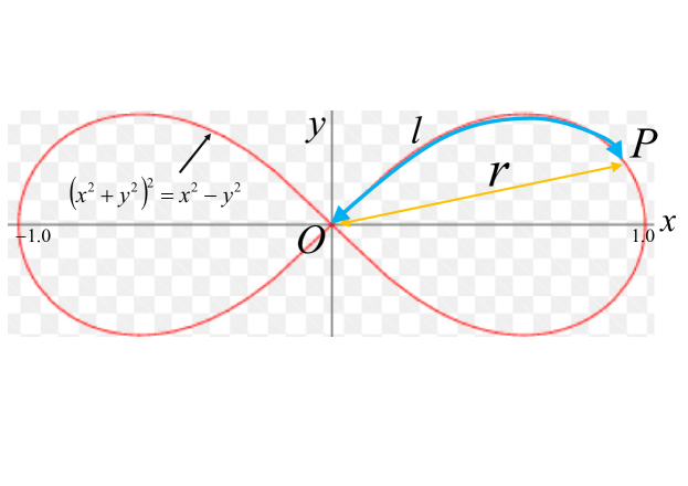
The leaf functions are closely related to the Jacobi elliptic functions. The Jacobi elliptic function originated from the lemniscate function. In 1691, Jacob Bernoulli noticed that the arc length OP of the lemniscate curve was the same as the integral of the equation[7]. As shown in Fig. 1, l𝑙l represents the length of arc OP. The arc OP is represented as:
Refer to caption
Figure 1: Lemniscate of Bernoulli
a​r​c​O​P=∫0rd​t1βˆ’t4(=l)π‘Žπ‘Ÿπ‘π‘‚π‘ƒannotatedsuperscriptsubscript0π‘Ÿd𝑑1superscript𝑑4absent𝑙arcOP=\int_{0}^{r}\frac{\mathrm{d}t}{\sqrt{1-t^{4}}}(=l) (25)

The curve in Fig. 1 can be expressed using variables xπ‘₯x and y𝑦y as:

(x2+y2)2=x2βˆ’y2superscriptsuperscriptπ‘₯2superscript𝑦22superscriptπ‘₯2superscript𝑦2(x^{2}+y^{2})^{2}=x^{2}-y^{2} (26)

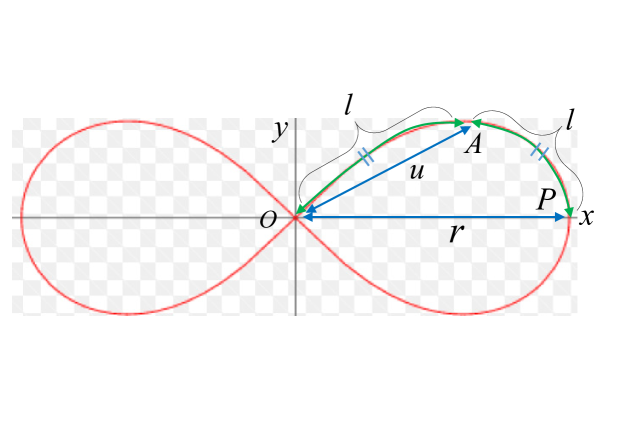
When the basis of the leaf function, n = 2, the curve for the leaf function is the same as the lemniscate curve. In 1718, Giulio Carlo de’ Toschi di Fagnano published a paper explaining how arc OP could be divided into two equal parts using only a straightedge and a compass[8]. He discovered that the length rπ‘Ÿr was twice the length u𝑒u, as shown in Fig. 2. This led to the derivation of the addition theorem for the lemniscate function:
Refer to caption
Figure 2: Fagnano and the Lemniscate
r=2​u​1βˆ’u41+u4​under​the​condition​a​r​c​O​P=2​a​r​c​O​Aπ‘Ÿ2𝑒1superscript𝑒41superscript𝑒4undertheconditionπ‘Žπ‘Ÿπ‘π‘‚π‘ƒ2π‘Žπ‘Ÿπ‘π‘‚π΄r=\frac{2u\sqrt{1-u^{4}}}{1+u^{4}}\>\mathrm{under}\>\mathrm{the}\>\mathrm{condition}\>arcOP=2arcOA (27)
a​r​c​O​A=∫0ud​t1βˆ’t4π‘Žπ‘Ÿπ‘π‘‚π΄superscriptsubscript0𝑒d𝑑1superscript𝑑4arcOA=\int_{0}^{u}\frac{\mathrm{d}t}{\sqrt{1-t^{4}}} (28)

After reading Fagnano’s paper, Leonhard Euler found the addition formula for the lemniscate function in 1752[9]. In the formula, the sum of the integral forms of arbitrary variables u𝑒u and v𝑣v equals the integral form rπ‘Ÿr:

r=u​1βˆ’v4+v​1βˆ’u41+u2​v2π‘Ÿπ‘’1superscript𝑣4𝑣1superscript𝑒41superscript𝑒2superscript𝑣2r=\frac{u\sqrt{1-v^{4}}+v\sqrt{1-u^{4}}}{1+u^{2}v^{2}} (29)

The above-mentioned relation satisfies the integral equation as follows:

∫0rd​t1βˆ’t4=∫0ud​t1βˆ’t4+∫0vd​t1βˆ’t4superscriptsubscript0π‘Ÿd𝑑1superscript𝑑4superscriptsubscript0𝑒d𝑑1superscript𝑑4superscriptsubscript0𝑣d𝑑1superscript𝑑4\int_{0}^{r}\frac{\mathrm{d}t}{\sqrt{1-t^{4}}}=\int_{0}^{u}\frac{\mathrm{d}t}{\sqrt{1-t^{4}}}+\int_{0}^{v}\frac{\mathrm{d}t}{\sqrt{1-t^{4}}} (30)

In 1796, Carl Friedrich Gauss derived the addition formula using the lemniscate function[3]. The inverse lemniscate function is expressed as:

arcsl​(r)=∫0rd​t1βˆ’t4(=l1​o​r​l2)arcslπ‘Ÿannotatedsuperscriptsubscript0π‘Ÿd𝑑1superscript𝑑4absentsubscript𝑙1π‘œπ‘Ÿsubscript𝑙2\mathrm{arcsl}(r)=\int_{0}^{r}\frac{\mathrm{d}t}{\sqrt{1-t^{4}}}(=l_{1}\>or\>l_{2}) (31)

Using this definition of inverse arc sl, the addition formula of lemniscate function sl​(l1+l2)slsubscript𝑙1subscript𝑙2\mathrm{sl}(l_{1}+l_{2}) is derived as:

sl​(l1+l2)=s​l​(l1)​1βˆ’s​l​(l2)4+s​l​(l2)​1βˆ’s​l​(l1)41+s​l​(l1)2​s​l​(l2)2slsubscript𝑙1subscript𝑙2𝑠𝑙subscript𝑙11𝑠𝑙superscriptsubscript𝑙24𝑠𝑙subscript𝑙21𝑠𝑙superscriptsubscript𝑙141𝑠𝑙superscriptsubscript𝑙12𝑠𝑙superscriptsubscript𝑙22\mathrm{sl}(l_{1}+l_{2})=\frac{sl(l_{1})\sqrt{1-sl(l_{2})^{4}}+sl(l_{2})\sqrt{1-sl(l_{1})^{4}}}{1+sl(l_{1})^{2}sl(l_{2})^{2}} (32)

Phases l1subscript𝑙1l_{1} or l2subscript𝑙2l_{2} of lemniscate function sl can be extended to complex variables iβ‹…l1⋅𝑖subscript𝑙1i\cdot l_{1} or iβ‹…l2⋅𝑖subscript𝑙2i\cdot l_{2}, respectively. In 1827, Carl Gustav Jacob Jacobi derived the inverses of the Jacobi elliptic functions[10]. To derive the formula, the term t2superscript𝑑2t^{2} is added to the root of the integrand denominator in Eq. (31):

arcsn​(r,k)=∫0rd​t1βˆ’(1+k2)​t2+k2​t4arcsnπ‘Ÿπ‘˜superscriptsubscript0π‘Ÿd𝑑11superscriptπ‘˜2superscript𝑑2superscriptπ‘˜2superscript𝑑4\mathrm{arcsn}(r,k)=\int_{0}^{r}\frac{\mathrm{d}t}{\sqrt{1-(1+k^{2})t^{2}+k^{2}t^{4}}} (33)

Eq. (33) represents the inverse Jacobi elliptic function sn, where kπ‘˜k is a constant. There exist 12 Jacobi elliptic functions, including cn and dn. In the Eq. (33), the variable t𝑑t is to the fourth power in the denominator. Jacobi did not discuss the variable t𝑑t to higher powers, such as follows:

∫0rd​t1βˆ’t6,∫0rd​t1βˆ’t8,∫0rd​t1βˆ’t10​…superscriptsubscript0π‘Ÿd𝑑1superscript𝑑6superscriptsubscript0π‘Ÿd𝑑1superscript𝑑8superscriptsubscript0π‘Ÿd𝑑1superscript𝑑10…\int_{0}^{r}\frac{\mathrm{d}t}{\sqrt{1-t^{6}}}\>,\>\int_{0}^{r}\frac{\mathrm{d}t}{\sqrt{1-t^{8}}}\>,\>\int_{0}^{r}\frac{\mathrm{d}t}{\sqrt{1-t^{10}}}\ldots\ (34)

In other words, there had been no discussion for n=3𝑛3n=3 in Eqs. (2), (3), (16), and (17). Therefore, the addition formulas for the leaf function were investigated for n=3[11]. In case of n≧3𝑛3n\geqq 3, no clear description for the addition formulas of hyperbolic leaf functions exists. On the contrary, n=1𝑛1n=1 represents hyperbolic functions sinh(l𝑙l) and cosh(l𝑙l). Therefore, the addition formulas of the hyperbolic leaf function and hyperbolic function are the same. The hyperbolic leaf function with n=2𝑛2n=2 represents hyperbolic lemniscate function slh(l𝑙l). No clear description of the addition formulas of function slh(l𝑙l) exists.

1.5 Advantage and Disadvantage

In physics, the nonlinear duffing equation represents a model for the spring pendulum whose spring stiffness does not obey Hooke’s law. This undamped duffing equation is represented as:

Cubicβˆ’Quintic​Duffing​Equation:d2​rd​l2+α​r+β​r3+μ​r5=0:CubicQuinticDuffingEquationsuperscriptd2π‘Ÿdsuperscript𝑙2π›Όπ‘Ÿπ›½superscriptπ‘Ÿ3πœ‡superscriptπ‘Ÿ50\mathrm{Cubic-Quintic\>Duffing\>Equation:}\frac{\mathrm{d}^{2}r}{\mathrm{d}l^{2}}+\alpha r+\beta r^{3}+\mu r^{5}=0 (35)

To solve the above equation, numerical analysis or analytical approximate solutions have been applied[12, 13, 14, 15, 16, 17, 18, 19, 20, 21, 22, 23, 24]. Additionally, literatures describe the application of the cubic duffing equation, using Jacobi elliptic functions[25, 26, 27]. As in the leaf function represented by Eq. (2), the term t2superscript𝑑2t^{2} is added to the root of inverse Jacobian elliptic function sn in Eq. (33). Variables rπ‘Ÿr and kπ‘˜k control Jacobian function sn. The scope of applying the duffing equation to the Jacobian elliptic function is wider compared with the leaf function that has only one parameter l𝑙l. Over time, the nonlinear duffing equation has witnessed improvements and further numerical analysis[28, 29, 30, 31].

Cubicβˆ’Quinticβˆ’Septic​Duffing​Equation:d2​rd​l2+α​r+β​r3+μ​r5+δ​r7=0:CubicQuinticSepticDuffingEquationsuperscriptd2π‘Ÿdsuperscript𝑙2π›Όπ‘Ÿπ›½superscriptπ‘Ÿ3πœ‡superscriptπ‘Ÿ5𝛿superscriptπ‘Ÿ70\mathrm{Cubic-Quintic-Septic\>Duffing\>Equation:}\frac{\mathrm{d}^{2}r}{\mathrm{d}l^{2}}+\alpha r+\beta r^{3}+\mu r^{5}+\delta r^{7}=0 (36)

A high-order exact solution using the Jacobi elliptic function has not been found yet. Furthermore, the high-order addition theorem necessary to derive the exact solution is not defined in the Jacobi elliptic function. To find the exact solution, it is key to determine if the superposition principle can be applied to linear equations. In the equations of various functions, mathematical operations divide one term into two or integrate two terms into one using the addition theorem. In this paper, we derive the addition theorem to further derive an exact solution for a high-order duffing equation, followed by applying the superposition principle.

2 Addition Formulas

2.1 Addition Formulas of Leaf Functions

Let there be two variables, l1subscript𝑙1l_{1} and l2subscript𝑙2l_{2}. The addition formulas of the function sleaf2​(l)subscriptsleaf2𝑙\mathrm{sleaf}_{2}(l) can be stated as follows:

sleaf2​(l1+l2)=sleaf2​(l1)β€‹βˆ‚sleaf2​(l2)βˆ‚l2+sleaf2​(l2)β€‹βˆ‚sleaf2​(l1)βˆ‚l11+(sleaf2​(l1))2​(sleaf2​(l2))2subscriptsleaf2subscript𝑙1subscript𝑙2subscriptsleaf2subscript𝑙1subscriptsleaf2subscript𝑙2subscript𝑙2subscriptsleaf2subscript𝑙2subscriptsleaf2subscript𝑙1subscript𝑙11superscriptsubscriptsleaf2subscript𝑙12superscriptsubscriptsleaf2subscript𝑙22\mathrm{sleaf}_{2}(l_{1}+l_{2})=\frac{\mathrm{sleaf}_{2}(l_{1})\frac{\mathrm{\partial}\mathrm{sleaf}_{2}(l_{2})}{\mathrm{\partial}l_{2}}+\mathrm{sleaf}_{2}(l_{2})\frac{\mathrm{\partial}\mathrm{sleaf}_{2}(l_{1})}{\mathrm{\partial}l_{1}}}{1+(\mathrm{sleaf}_{2}(l_{1}))^{2}(\mathrm{sleaf}_{2}(l_{2}))^{2}} (37)

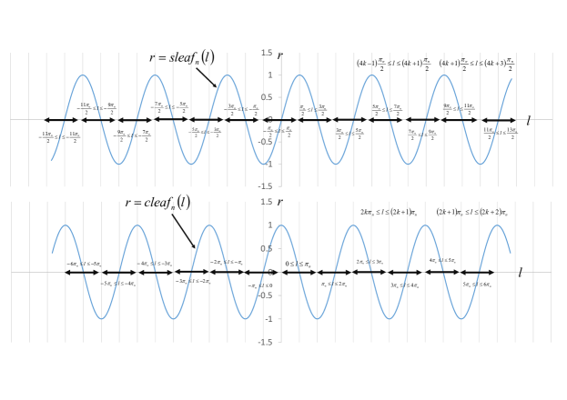
Depending on the domain of the variable l𝑙l of the leaf function, the signs of both βˆ‚sleaf2​(l2)/βˆ‚l2subscriptsleaf2subscript𝑙2subscript𝑙2\mathrm{\partial}\mathrm{sleaf}_{2}(l_{2})/\mathrm{\partial}l_{2} and βˆ‚sleaf2​(l1)/βˆ‚l1subscriptsleaf2subscript𝑙1subscript𝑙1\mathrm{\partial}\mathrm{sleaf}_{2}(l_{1})/\mathrm{\partial}l_{1} change. Eq. (37) can be summarized according a number of cases based on the domains of variables l1subscript𝑙1l_{1} and l2subscript𝑙2l_{2}(See Figure 3). The parameters mπ‘šm and kπ‘˜k represent integers.

(i) In the case where Ο€22​(4​mβˆ’1)≦l1≦π22​(4​m+1)subscriptπœ‹224π‘š1subscript𝑙1subscriptπœ‹224π‘š1\frac{\pi_{2}}{2}(4m-1)\leqq l_{1}\leqq\frac{\pi_{2}}{2}(4m+1), Ο€22​(4​kβˆ’1)≦l2≦π22​(4​k+1)subscriptπœ‹224π‘˜1subscript𝑙2subscriptπœ‹224π‘˜1\frac{\pi_{2}}{2}(4k-1)\leqq l_{2}\leqq\frac{\pi_{2}}{2}(4k+1)(see Appendix E for the constant Ο€2subscriptπœ‹2\pi_{2}), Eq. (37) is transformed into:

sleaf2​(l1+l2)=sleaf2​(l1)​1βˆ’(sleaf2​(l2))4+sleaf2​(l2)​1βˆ’(sleaf2​(l1))41+(sleaf2​(l1))2​(sleaf2​(l2))2subscriptsleaf2subscript𝑙1subscript𝑙2subscriptsleaf2subscript𝑙11superscriptsubscriptsleaf2subscript𝑙24subscriptsleaf2subscript𝑙21superscriptsubscriptsleaf2subscript𝑙141superscriptsubscriptsleaf2subscript𝑙12superscriptsubscriptsleaf2subscript𝑙22\mathrm{sleaf}_{2}(l_{1}+l_{2})=\frac{\mathrm{sleaf}_{2}(l_{1})\sqrt{1-(\mathrm{sleaf}_{2}(l_{2}))^{4}}+\mathrm{sleaf}_{2}(l_{2})\sqrt{1-(\mathrm{sleaf}_{2}(l_{1}))^{4}}}{1+(\mathrm{sleaf}_{2}(l_{1}))^{2}(\mathrm{sleaf}_{2}(l_{2}))^{2}} (38)

(ii) In the case where Ο€22​(4​mβˆ’1)≦l1≦π22​(4​m+1)subscriptπœ‹224π‘š1subscript𝑙1subscriptπœ‹224π‘š1\frac{\pi_{2}}{2}(4m-1)\leqq l_{1}\leqq\frac{\pi_{2}}{2}(4m+1), Ο€22​(4​k+1)≦l2≦π22​(4​k+3)subscriptπœ‹224π‘˜1subscript𝑙2subscriptπœ‹224π‘˜3\frac{\pi_{2}}{2}(4k+1)\leqq l_{2}\leqq\frac{\pi_{2}}{2}(4k+3), Eq. (37) is transformed into:

sleaf2​(l1+l2)=βˆ’sleaf2​(l1)​1βˆ’(sleaf2​(l2))4+sleaf2​(l2)​1βˆ’(sleaf2​(l1))41+(sleaf2​(l1))2​(sleaf2​(l2))2subscriptsleaf2subscript𝑙1subscript𝑙2subscriptsleaf2subscript𝑙11superscriptsubscriptsleaf2subscript𝑙24subscriptsleaf2subscript𝑙21superscriptsubscriptsleaf2subscript𝑙141superscriptsubscriptsleaf2subscript𝑙12superscriptsubscriptsleaf2subscript𝑙22\mathrm{sleaf}_{2}(l_{1}+l_{2})=\frac{-\mathrm{sleaf}_{2}(l_{1})\sqrt{1-(\mathrm{sleaf}_{2}(l_{2}))^{4}}+\mathrm{sleaf}_{2}(l_{2})\sqrt{1-(\mathrm{sleaf}_{2}(l_{1}))^{4}}}{1+(\mathrm{sleaf}_{2}(l_{1}))^{2}(\mathrm{sleaf}_{2}(l_{2}))^{2}} (39)

(iii) In the case where Ο€22​(4​m+1)≦l1≦π22​(4​m+3)subscriptπœ‹224π‘š1subscript𝑙1subscriptπœ‹224π‘š3\frac{\pi_{2}}{2}(4m+1)\leqq l_{1}\leqq\frac{\pi_{2}}{2}(4m+3), Ο€22​(4​kβˆ’1)≦l2≦π22​(4​k+1)subscriptπœ‹224π‘˜1subscript𝑙2subscriptπœ‹224π‘˜1\frac{\pi_{2}}{2}(4k-1)\leqq l_{2}\leqq\frac{\pi_{2}}{2}(4k+1), Eq. (37) is tansformed into:

sleaf2​(l1+l2)=sleaf2​(l1)​1βˆ’(sleaf2​(l2))4βˆ’sleaf2​(l2)​1βˆ’(sleaf2​(l1))41+(sleaf2​(l1))2​(sleaf2​(l2))2subscriptsleaf2subscript𝑙1subscript𝑙2subscriptsleaf2subscript𝑙11superscriptsubscriptsleaf2subscript𝑙24subscriptsleaf2subscript𝑙21superscriptsubscriptsleaf2subscript𝑙141superscriptsubscriptsleaf2subscript𝑙12superscriptsubscriptsleaf2subscript𝑙22\mathrm{sleaf}_{2}(l_{1}+l_{2})=\frac{\mathrm{sleaf}_{2}(l_{1})\sqrt{1-(\mathrm{sleaf}_{2}(l_{2}))^{4}}-\mathrm{sleaf}_{2}(l_{2})\sqrt{1-(\mathrm{sleaf}_{2}(l_{1}))^{4}}}{1+(\mathrm{sleaf}_{2}(l_{1}))^{2}(\mathrm{sleaf}_{2}(l_{2}))^{2}} (40)

(iiii) In the case where Ο€22​(4​m+1)≦l1≦π22​(4​m+3)subscriptπœ‹224π‘š1subscript𝑙1subscriptπœ‹224π‘š3\frac{\pi_{2}}{2}(4m+1)\leqq l_{1}\leqq\frac{\pi_{2}}{2}(4m+3), Ο€22​(4​k+1)≦l2≦π22​(4​k+3)subscriptπœ‹224π‘˜1subscript𝑙2subscriptπœ‹224π‘˜3\frac{\pi_{2}}{2}(4k+1)\leqq l_{2}\leqq\frac{\pi_{2}}{2}(4k+3), Eq. (37) is tansformed into:

sleaf2​(l1+l2)=βˆ’sleaf2​(l1)​1βˆ’(sleaf2​(l2))4βˆ’sleaf2​(l2)​1βˆ’(sleaf2​(l1))41+(sleaf2​(l1))2​(sleaf2​(l2))2subscriptsleaf2subscript𝑙1subscript𝑙2subscriptsleaf2subscript𝑙11superscriptsubscriptsleaf2subscript𝑙24subscriptsleaf2subscript𝑙21superscriptsubscriptsleaf2subscript𝑙141superscriptsubscriptsleaf2subscript𝑙12superscriptsubscriptsleaf2subscript𝑙22\mathrm{sleaf}_{2}(l_{1}+l_{2})=\frac{-\mathrm{sleaf}_{2}(l_{1})\sqrt{1-(\mathrm{sleaf}_{2}(l_{2}))^{4}}-\mathrm{sleaf}_{2}(l_{2})\sqrt{1-(\mathrm{sleaf}_{2}(l_{1}))^{4}}}{1+(\mathrm{sleaf}_{2}(l_{1}))^{2}(\mathrm{sleaf}_{2}(l_{2}))^{2}} (41)

Next, the addition formula of cleaf2​(l)subscriptcleaf2𝑙\mathrm{cleaf}_{2}(l) can be stated as follows:

cleaf2​(l1+l2)=cleaf2​(l1)β€‹βˆ‚sleaf2​(l2)βˆ‚l2+sleaf2​(l2)β€‹βˆ‚cleaf2​(l1)βˆ‚l11+(cleaf2​(l1))2​(sleaf2​(l2))2subscriptcleaf2subscript𝑙1subscript𝑙2subscriptcleaf2subscript𝑙1subscriptsleaf2subscript𝑙2subscript𝑙2subscriptsleaf2subscript𝑙2subscriptcleaf2subscript𝑙1subscript𝑙11superscriptsubscriptcleaf2subscript𝑙12superscriptsubscriptsleaf2subscript𝑙22\mathrm{cleaf}_{2}(l_{1}+l_{2})=\frac{\mathrm{cleaf}_{2}(l_{1})\frac{\mathrm{\partial sleaf}_{2}(l_{2})}{\mathrm{\partial}l_{2}}+\mathrm{sleaf}_{2}(l_{2})\frac{\mathrm{\partial cleaf}_{2}(l_{1})}{\mathrm{\partial}l_{1}}}{1+(\mathrm{cleaf}_{2}(l_{1}))^{2}(\mathrm{sleaf}_{2}(l_{2}))^{2}} (42)

Depending on the domain of the variable l𝑙l of the leaf function, the signs of both βˆ‚sleaf2​(l2)/βˆ‚l2subscriptsleaf2subscript𝑙2subscript𝑙2\mathrm{\partial sleaf}_{2}(l_{2})/\mathrm{\partial}l_{2} and βˆ‚cleaf2​(l1)/βˆ‚l1subscriptcleaf2subscript𝑙1subscript𝑙1\mathrm{\partial cleaf}_{2}(l_{1})/\mathrm{\partial}l_{1} change. Eq. (42) can be summarized according a number of cases based on the domains of variables l1subscript𝑙1l_{1} and l2subscript𝑙2l_{2}.

(i) In the case where 2​m​π2≦l1≦(2​m+1)​π22π‘šsubscriptπœ‹2subscript𝑙12π‘š1subscriptπœ‹22m\pi_{2}\leqq l_{1}\leqq(2m+1)\pi_{2}, Ο€22​(4​kβˆ’1)≦l2≦π22​(4​k+1)subscriptπœ‹224π‘˜1subscript𝑙2subscriptπœ‹224π‘˜1\frac{\pi_{2}}{2}(4k-1)\leqq l_{2}\leqq\frac{\pi_{2}}{2}(4k+1), Eq. (42) is transformed into:

cleaf2​(l1+l2)=cleaf2​(l1)​1βˆ’(sleaf2​(l2))4βˆ’sleaf2​(l2)​1βˆ’(cleaf2​(l1))41+(cleaf2​(l1))2​(sleaf2​(l2))2subscriptcleaf2subscript𝑙1subscript𝑙2subscriptcleaf2subscript𝑙11superscriptsubscriptsleaf2subscript𝑙24subscriptsleaf2subscript𝑙21superscriptsubscriptcleaf2subscript𝑙141superscriptsubscriptcleaf2subscript𝑙12superscriptsubscriptsleaf2subscript𝑙22\mathrm{cleaf}_{2}(l_{1}+l_{2})=\frac{\mathrm{cleaf}_{2}(l_{1})\sqrt{1-(\mathrm{sleaf}_{2}(l_{2}))^{4}}-\mathrm{sleaf}_{2}(l_{2})\sqrt{1-(\mathrm{cleaf}_{2}(l_{1}))^{4}}}{1+(\mathrm{cleaf}_{2}(l_{1}))^{2}(\mathrm{sleaf}_{2}(l_{2}))^{2}} (43)

(ii) In the case where (2​mβˆ’1)​π2≦l1≦2​m​π22π‘š1subscriptπœ‹2subscript𝑙12π‘šsubscriptπœ‹2(2m-1)\pi_{2}\leqq l_{1}\leqq 2m\pi_{2}, Ο€22​(4​kβˆ’1)≦l2≦π22​(4​k+1)subscriptπœ‹224π‘˜1subscript𝑙2subscriptπœ‹224π‘˜1\frac{\pi_{2}}{2}(4k-1)\leqq l_{2}\leqq\frac{\pi_{2}}{2}(4k+1), Eq. (42) is transformed into:

cleaf2​(l1+l2)=cleaf2​(l1)​1βˆ’(sleaf2​(l2))4+sleaf2​(l2)​1βˆ’(cleaf2​(l1))41+(cleaf2​(l1))2​(sleaf2​(l2))2subscriptcleaf2subscript𝑙1subscript𝑙2subscriptcleaf2subscript𝑙11superscriptsubscriptsleaf2subscript𝑙24subscriptsleaf2subscript𝑙21superscriptsubscriptcleaf2subscript𝑙141superscriptsubscriptcleaf2subscript𝑙12superscriptsubscriptsleaf2subscript𝑙22\mathrm{cleaf}_{2}(l_{1}+l_{2})=\frac{\mathrm{cleaf}_{2}(l_{1})\sqrt{1-(\mathrm{sleaf}_{2}(l_{2}))^{4}}+\mathrm{sleaf}_{2}(l_{2})\sqrt{1-(\mathrm{cleaf}_{2}(l_{1}))^{4}}}{1+(\mathrm{cleaf}_{2}(l_{1}))^{2}(\mathrm{sleaf}_{2}(l_{2}))^{2}} (44)

(iii) In the case where (2​mβˆ’1)​π2≦l1≦2​m​π22π‘š1subscriptπœ‹2subscript𝑙12π‘šsubscriptπœ‹2(2m-1)\pi_{2}\leqq l_{1}\leqq 2m\pi_{2}, Ο€22​(4​k+1)≦l2≦π22​(4​k+3)subscriptπœ‹224π‘˜1subscript𝑙2subscriptπœ‹224π‘˜3\frac{\pi_{2}}{2}(4k+1)\leqq l_{2}\leqq\frac{\pi_{2}}{2}(4k+3), Eq. (42) is transformed into:

cleaf2​(l1+l2)=βˆ’cleaf2​(l1)​1βˆ’(sleaf2​(l2))4+sleaf2​(l2)​1βˆ’(cleaf2​(l1))41+(cleaf2​(l1))2​(sleaf2​(l2))2subscriptcleaf2subscript𝑙1subscript𝑙2subscriptcleaf2subscript𝑙11superscriptsubscriptsleaf2subscript𝑙24subscriptsleaf2subscript𝑙21superscriptsubscriptcleaf2subscript𝑙141superscriptsubscriptcleaf2subscript𝑙12superscriptsubscriptsleaf2subscript𝑙22\mathrm{cleaf}_{2}(l_{1}+l_{2})=\frac{-\mathrm{cleaf}_{2}(l_{1})\sqrt{1-(\mathrm{sleaf}_{2}(l_{2}))^{4}}+\mathrm{sleaf}_{2}(l_{2})\sqrt{1-(\mathrm{cleaf}_{2}(l_{1}))^{4}}}{1+(\mathrm{cleaf}_{2}(l_{1}))^{2}(\mathrm{sleaf}_{2}(l_{2}))^{2}} (45)

(iiii) In the case where 2​m​π2≦l1≦(2​m+1)​π22π‘šsubscriptπœ‹2subscript𝑙12π‘š1subscriptπœ‹22m\pi_{2}\leqq l_{1}\leqq(2m+1)\pi_{2}, Ο€22​(4​k+1)≦l2≦π22​(4​k+3)subscriptπœ‹224π‘˜1subscript𝑙2subscriptπœ‹224π‘˜3\frac{\pi_{2}}{2}(4k+1)\leqq l_{2}\leqq\frac{\pi_{2}}{2}(4k+3), Eq. (42) is transformed into:

cleaf2​(l1+l2)=βˆ’cleaf2​(l1)​1βˆ’(sleaf2​(l2))4βˆ’sleaf2​(l2)​1βˆ’(cleaf2​(l1))41+(cleaf2​(l1))2​(sleaf2​(l2))2subscriptcleaf2subscript𝑙1subscript𝑙2subscriptcleaf2subscript𝑙11superscriptsubscriptsleaf2subscript𝑙24subscriptsleaf2subscript𝑙21superscriptsubscriptcleaf2subscript𝑙141superscriptsubscriptcleaf2subscript𝑙12superscriptsubscriptsleaf2subscript𝑙22\mathrm{cleaf}_{2}(l_{1}+l_{2})=\frac{-\mathrm{cleaf}_{2}(l_{1})\sqrt{1-(\mathrm{sleaf}_{2}(l_{2}))^{4}}-\mathrm{sleaf}_{2}(l_{2})\sqrt{1-(\mathrm{cleaf}_{2}(l_{1}))^{4}}}{1+(\mathrm{cleaf}_{2}(l_{1}))^{2}(\mathrm{sleaf}_{2}(l_{2}))^{2}} (46)

Next, the addition formulas of sleaf3​(l)subscriptsleaf3𝑙\mathrm{sleaf}_{3}(l) can be described as follows:

(sleaf3​(l1+l2))2={sleaf3​(l1)β€‹βˆ‚sleaf3​(l2)βˆ‚l2+sleaf3​(l2)β€‹βˆ‚sleaf3​(l1)βˆ‚l1}21+4​(sleaf3​(l1))4​(sleaf3​(l2))2+4​(sleaf3​(l1))2​(sleaf3​(l2))4+{(sleaf3​(l1))3​sleaf3​(l2)βˆ’sleaf3​(l1)​(sleaf3​(l2))3}21+4​(sleaf3​(l1))4​(sleaf3​(l2))2+4​(sleaf3​(l1))2​(sleaf3​(l2))4superscriptsubscriptsleaf3subscript𝑙1subscript𝑙22superscriptsubscriptsleaf3subscript𝑙1subscriptsleaf3subscript𝑙2subscript𝑙2subscriptsleaf3subscript𝑙2subscriptsleaf3subscript𝑙1subscript𝑙1214superscriptsubscriptsleaf3subscript𝑙14superscriptsubscriptsleaf3subscript𝑙224superscriptsubscriptsleaf3subscript𝑙12superscriptsubscriptsleaf3subscript𝑙24superscriptsuperscriptsubscriptsleaf3subscript𝑙13subscriptsleaf3subscript𝑙2subscriptsleaf3subscript𝑙1superscriptsubscriptsleaf3subscript𝑙23214superscriptsubscriptsleaf3subscript𝑙14superscriptsubscriptsleaf3subscript𝑙224superscriptsubscriptsleaf3subscript𝑙12superscriptsubscriptsleaf3subscript𝑙24\begin{split}(\mathrm{sleaf}_{3}(l_{1}+l_{2}))^{2}=\frac{\left\{\mathrm{sleaf}_{3}(l_{1})\frac{\mathrm{\partial sleaf}_{3}(l_{2})}{\mathrm{\partial}l_{2}}+\mathrm{sleaf}_{3}(l_{2})\frac{\mathrm{\partial sleaf}_{3}(l_{1})}{\mathrm{\partial}l_{1}}\right\}^{2}}{1+4(\mathrm{sleaf}_{3}(l_{1}))^{4}(\mathrm{sleaf}_{3}(l_{2}))^{2}+4(\mathrm{sleaf}_{3}(l_{1}))^{2}(\mathrm{sleaf}_{3}(l_{2}))^{4}}\\ +\frac{\left\{(\mathrm{sleaf}_{3}(l_{1}))^{3}\mathrm{sleaf}_{3}(l_{2})-\mathrm{sleaf}_{3}(l_{1})(\mathrm{sleaf}_{3}(l_{2}))^{3}\right\}^{2}}{1+4(\mathrm{sleaf}_{3}(l_{1}))^{4}(\mathrm{sleaf}_{3}(l_{2}))^{2}+4(\mathrm{sleaf}_{3}(l_{1}))^{2}(\mathrm{sleaf}_{3}(l_{2}))^{4}}\end{split} (47)

The preceding equation can be summarized as follows according to a number of cases based on the domains of the variables l1subscript𝑙1l_{1} and l2subscript𝑙2l_{2}.

(i) In the case where both (4​mβˆ’1)​π32≦l1≦(4​m+1)​π324π‘š1subscriptπœ‹32subscript𝑙14π‘š1subscriptπœ‹32(4m-1)\frac{\pi_{3}}{2}\leqq l_{1}\leqq(4m+1)\frac{\pi_{3}}{2} and (4​kβˆ’1)​π32≦l2≦(4​k+1)​π324π‘˜1subscriptπœ‹32subscript𝑙24π‘˜1subscriptπœ‹32(4k-1)\frac{\pi_{3}}{2}\leqq l_{2}\leqq(4k+1)\frac{\pi_{3}}{2} or both (4​m+1)​π32≦l1≦(4​m+3)​π324π‘š1subscriptπœ‹32subscript𝑙14π‘š3subscriptπœ‹32(4m+1)\frac{\pi_{3}}{2}\leqq l_{1}\leqq(4m+3)\frac{\pi_{3}}{2} and (4​k+1)​π32≦l2≦(4​k+3)​π324π‘˜1subscriptπœ‹32subscript𝑙24π‘˜3subscriptπœ‹32(4k+1)\frac{\pi_{3}}{2}\leqq l_{2}\leqq(4k+3)\frac{\pi_{3}}{2}, Eq. (47) is tansformed into:

(sleaf3​(l1+l2))2={sleaf3​(l1)​1βˆ’(sleaf3​(l2))6+sleaf3​(l2)​1βˆ’(sleaf3​(l1))6}21+4​(sleaf3​(l1))4​(sleaf3​(l2))2+4​(sleaf3​(l1))2​(sleaf3​(l2))4+{(sleaf3​(l1))3​sleaf3​(l2)βˆ’sleaf3​(l1)​(sleaf3​(l2))3}21+4​(sleaf3​(l1))4​(sleaf3​(l2))2+4​(sleaf3​(l1))2​(sleaf3​(l2))4superscriptsubscriptsleaf3subscript𝑙1subscript𝑙22superscriptsubscriptsleaf3subscript𝑙11superscriptsubscriptsleaf3subscript𝑙26subscriptsleaf3subscript𝑙21superscriptsubscriptsleaf3subscript𝑙16214superscriptsubscriptsleaf3subscript𝑙14superscriptsubscriptsleaf3subscript𝑙224superscriptsubscriptsleaf3subscript𝑙12superscriptsubscriptsleaf3subscript𝑙24superscriptsuperscriptsubscriptsleaf3subscript𝑙13subscriptsleaf3subscript𝑙2subscriptsleaf3subscript𝑙1superscriptsubscriptsleaf3subscript𝑙23214superscriptsubscriptsleaf3subscript𝑙14superscriptsubscriptsleaf3subscript𝑙224superscriptsubscriptsleaf3subscript𝑙12superscriptsubscriptsleaf3subscript𝑙24\begin{split}(\mathrm{sleaf}_{3}(l_{1}+l_{2}))^{2}=\frac{\left\{\mathrm{sleaf}_{3}(l_{1})\sqrt{1-(\mathrm{sleaf}_{3}(l_{2}))^{6}}+\mathrm{sleaf}_{3}(l_{2})\sqrt{1-(\mathrm{sleaf}_{3}(l_{1}))^{6}}\right\}^{2}}{1+4(\mathrm{sleaf}_{3}(l_{1}))^{4}(\mathrm{sleaf}_{3}(l_{2}))^{2}+4(\mathrm{sleaf}_{3}(l_{1}))^{2}(\mathrm{sleaf}_{3}(l_{2}))^{4}}\\ +\frac{\left\{(\mathrm{sleaf}_{3}(l_{1}))^{3}\mathrm{sleaf}_{3}(l_{2})-\mathrm{sleaf}_{3}(l_{1})(\mathrm{sleaf}_{3}(l_{2}))^{3}\right\}^{2}}{1+4(\mathrm{sleaf}_{3}(l_{1}))^{4}(\mathrm{sleaf}_{3}(l_{2}))^{2}+4(\mathrm{sleaf}_{3}(l_{1}))^{2}(\mathrm{sleaf}_{3}(l_{2}))^{4}}\end{split} (48)

The symbol Ο€3subscriptπœ‹3\pi_{3} represents a constant (see Appendix E).

(ii) In the case where both (4​m+1)​π32≦l1≦(4​m+3)​π324π‘š1subscriptπœ‹32subscript𝑙14π‘š3subscriptπœ‹32(4m+1)\frac{\pi_{3}}{2}\leqq l_{1}\leqq(4m+3)\frac{\pi_{3}}{2} and (4​kβˆ’1)​π32≦l2≦(4​k+1)​π324π‘˜1subscriptπœ‹32subscript𝑙24π‘˜1subscriptπœ‹32(4k-1)\frac{\pi_{3}}{2}\leqq l_{2}\leqq(4k+1)\frac{\pi_{3}}{2} or both (4​mβˆ’1)​π32≦l1≦(4​m+1)​π324π‘š1subscriptπœ‹32subscript𝑙14π‘š1subscriptπœ‹32(4m-1)\frac{\pi_{3}}{2}\leqq l_{1}\leqq(4m+1)\frac{\pi_{3}}{2} and (4​k+1)​π32≦l2≦(4​k+3)​π324π‘˜1subscriptπœ‹32subscript𝑙24π‘˜3subscriptπœ‹32(4k+1)\frac{\pi_{3}}{2}\leqq l_{2}\leqq(4k+3)\frac{\pi_{3}}{2}, Eq. (47) is tansformed into:

(sleaf3​(l1+l2))2={sleaf3​(l1)​1βˆ’(sleaf3​(l2))6βˆ’sleaf3​(l2)​1βˆ’(sleaf3​(l1))6}21+4​(sleaf3​(l1))4​(sleaf3​(l2))2+4​(sleaf3​(l1))2​(sleaf3​(l2))4+{(sleaf3​(l1))3​sleaf3​(l2)βˆ’sleaf3​(l1)​(sleaf3​(l2))3}21+4​(sleaf3​(l1))4​(sleaf3​(l2))2+4​(sleaf3​(l1))2​(sleaf3​(l2))4superscriptsubscriptsleaf3subscript𝑙1subscript𝑙22superscriptsubscriptsleaf3subscript𝑙11superscriptsubscriptsleaf3subscript𝑙26subscriptsleaf3subscript𝑙21superscriptsubscriptsleaf3subscript𝑙16214superscriptsubscriptsleaf3subscript𝑙14superscriptsubscriptsleaf3subscript𝑙224superscriptsubscriptsleaf3subscript𝑙12superscriptsubscriptsleaf3subscript𝑙24superscriptsuperscriptsubscriptsleaf3subscript𝑙13subscriptsleaf3subscript𝑙2subscriptsleaf3subscript𝑙1superscriptsubscriptsleaf3subscript𝑙23214superscriptsubscriptsleaf3subscript𝑙14superscriptsubscriptsleaf3subscript𝑙224superscriptsubscriptsleaf3subscript𝑙12superscriptsubscriptsleaf3subscript𝑙24\begin{split}(\mathrm{sleaf}_{3}(l_{1}+l_{2}))^{2}=\frac{\left\{\mathrm{sleaf}_{3}(l_{1})\sqrt{1-(\mathrm{sleaf}_{3}(l_{2}))^{6}}-\mathrm{sleaf}_{3}(l_{2})\sqrt{1-(\mathrm{sleaf}_{3}(l_{1}))^{6}}\right\}^{2}}{1+4(\mathrm{sleaf}_{3}(l_{1}))^{4}(\mathrm{sleaf}_{3}(l_{2}))^{2}+4(\mathrm{sleaf}_{3}(l_{1}))^{2}(\mathrm{sleaf}_{3}(l_{2}))^{4}}\\ +\frac{\left\{(\mathrm{sleaf}_{3}(l_{1}))^{3}\mathrm{sleaf}_{3}(l_{2})-\mathrm{sleaf}_{3}(l_{1})(\mathrm{sleaf}_{3}(l_{2}))^{3}\right\}^{2}}{1+4(\mathrm{sleaf}_{3}(l_{1}))^{4}(\mathrm{sleaf}_{3}(l_{2}))^{2}+4(\mathrm{sleaf}_{3}(l_{1}))^{2}(\mathrm{sleaf}_{3}(l_{2}))^{4}}\end{split} (49)

Next, the addition formulas of cleaf3​(l)subscriptcleaf3𝑙\mathrm{cleaf}_{3}(l) can be defined as follows:

(cleaf3​(l1+l2))2={cleaf3​(l1)β€‹βˆ‚sleaf3​(l2)βˆ‚l2+sleaf3​(l2)β€‹βˆ‚cleaf3​(l1)βˆ‚l1}21+4​(sleaf3​(l2))4​(cleaf3​(l1))2+4​(sleaf3​(l2))2​(cleaf3​(l1))4+{(sleaf3​(l2))3​cleaf3​(l1)βˆ’sleaf3​(l2)​(cleaf3​(l1))3}21+4​(sleaf3​(l2))4​(cleaf3​(l1))2+4​(sleaf3​(l2))2​(cleaf3​(l1))4superscriptsubscriptcleaf3subscript𝑙1subscript𝑙22superscriptsubscriptcleaf3subscript𝑙1subscriptsleaf3subscript𝑙2subscript𝑙2subscriptsleaf3subscript𝑙2subscriptcleaf3subscript𝑙1subscript𝑙1214superscriptsubscriptsleaf3subscript𝑙24superscriptsubscriptcleaf3subscript𝑙124superscriptsubscriptsleaf3subscript𝑙22superscriptsubscriptcleaf3subscript𝑙14superscriptsuperscriptsubscriptsleaf3subscript𝑙23subscriptcleaf3subscript𝑙1subscriptsleaf3subscript𝑙2superscriptsubscriptcleaf3subscript𝑙13214superscriptsubscriptsleaf3subscript𝑙24superscriptsubscriptcleaf3subscript𝑙124superscriptsubscriptsleaf3subscript𝑙22superscriptsubscriptcleaf3subscript𝑙14\begin{split}(\mathrm{cleaf}_{3}(l_{1}+l_{2}))^{2}=\frac{\left\{\mathrm{cleaf}_{3}(l_{1})\frac{\mathrm{\partial sleaf}_{3}(l_{2})}{\mathrm{\partial}l_{2}}+\mathrm{sleaf}_{3}(l_{2})\frac{\mathrm{\partial cleaf}_{3}(l_{1})}{\mathrm{\partial}l_{1}}\right\}^{2}}{1+4(\mathrm{sleaf}_{3}(l_{2}))^{4}(\mathrm{cleaf}_{3}(l_{1}))^{2}+4(\mathrm{sleaf}_{3}(l_{2}))^{2}(\mathrm{cleaf}_{3}(l_{1}))^{4}}\\ +\frac{\left\{(\mathrm{sleaf}_{3}(l_{2}))^{3}\mathrm{cleaf}_{3}(l_{1})-\mathrm{sleaf}_{3}(l_{2})(\mathrm{cleaf}_{3}(l_{1}))^{3}\right\}^{2}}{1+4(\mathrm{sleaf}_{3}(l_{2}))^{4}(\mathrm{cleaf}_{3}(l_{1}))^{2}+4(\mathrm{sleaf}_{3}(l_{2}))^{2}(\mathrm{cleaf}_{3}(l_{1}))^{4}}\end{split} (50)

The preceding equation can be summarized as follows according to a number of cases based on the domains of the variables l1subscript𝑙1l_{1} and l2subscript𝑙2l_{2}.

(i) In the case where both 2​k​π3≦l1≦(2​k+1)​π32π‘˜subscriptπœ‹3subscript𝑙12π‘˜1subscriptπœ‹32k\pi_{3}\leqq l_{1}\leqq(2k+1)\pi_{3} and (4​mβˆ’1)​π32≦l2≦(4​m+1)​π324π‘š1subscriptπœ‹32subscript𝑙24π‘š1subscriptπœ‹32(4m-1)\frac{\pi_{3}}{2}\leqq l_{2}\leqq(4m+1)\frac{\pi_{3}}{2} or both (2​k+1)​π3≦l1≦(2​k+2)​π32π‘˜1subscriptπœ‹3subscript𝑙12π‘˜2subscriptπœ‹3(2k+1)\pi_{3}\leqq l_{1}\leqq(2k+2)\pi_{3} and (4​m+1)​π32≦l2≦(4​m+3)​π324π‘š1subscriptπœ‹32subscript𝑙24π‘š3subscriptπœ‹32(4m+1)\frac{\pi_{3}}{2}\leqq l_{2}\leqq(4m+3)\frac{\pi_{3}}{2}, Eq. (50) is transformed into:

(cleaf3​(l1+l2))2={cleaf3​(l1)​1βˆ’(sleaf3​(l2))6βˆ’sleaf3​(l2)​1βˆ’(cleaf3​(l1))6}21+4​(sleaf3​(l2))4​(cleaf3​(l1))2+4​(s​l​e​a​f3​(l2))2​(cleaf3​(l1))4+{(sleaf3​(l2))3​cleaf3​(l1)βˆ’sleaf3​(l2)​(cleaf3​(l1))3}21+4​(sleaf3​(l2))4​(cleaf3​(l1))2+4​(sleaf3​(l2))2​(cleaf3​(l1))4superscriptsubscriptcleaf3subscript𝑙1subscript𝑙22superscriptsubscriptcleaf3subscript𝑙11superscriptsubscriptsleaf3subscript𝑙26subscriptsleaf3subscript𝑙21superscriptsubscriptcleaf3subscript𝑙16214superscriptsubscriptsleaf3subscript𝑙24superscriptsubscriptcleaf3subscript𝑙124superscriptπ‘ π‘™π‘’π‘Žsubscript𝑓3subscript𝑙22superscriptsubscriptcleaf3subscript𝑙14superscriptsuperscriptsubscriptsleaf3subscript𝑙23subscriptcleaf3subscript𝑙1subscriptsleaf3subscript𝑙2superscriptsubscriptcleaf3subscript𝑙13214superscriptsubscriptsleaf3subscript𝑙24superscriptsubscriptcleaf3subscript𝑙124superscriptsubscriptsleaf3subscript𝑙22superscriptsubscriptcleaf3subscript𝑙14\begin{split}(\mathrm{cleaf}_{3}(l_{1}+l_{2}))^{2}=\frac{\left\{\mathrm{cleaf}_{3}(l_{1})\sqrt{1-(\mathrm{sleaf}_{3}(l_{2}))^{6}}-\mathrm{sleaf}_{3}(l_{2})\sqrt{1-(\mathrm{cleaf}_{3}(l_{1}))^{6}}\right\}^{2}}{1+4(\mathrm{sleaf}_{3}(l_{2}))^{4}(\mathrm{cleaf}_{3}(l_{1}))^{2}+4(sleaf_{3}(l_{2}))^{2}(\mathrm{cleaf}_{3}(l_{1}))^{4}}\\ +\frac{\left\{(\mathrm{sleaf}_{3}(l_{2}))^{3}\mathrm{cleaf}_{3}(l_{1})-\mathrm{sleaf}_{3}(l_{2})(\mathrm{cleaf}_{3}(l_{1}))^{3}\right\}^{2}}{1+4(\mathrm{sleaf}_{3}(l_{2}))^{4}(\mathrm{cleaf}_{3}(l_{1}))^{2}+4(\mathrm{sleaf}_{3}(l_{2}))^{2}(\mathrm{cleaf}_{3}(l_{1}))^{4}}\end{split} (51)

(ii) In the case where both (2​k+1)​π3≦l1≦(2​k+2)​π32π‘˜1subscriptπœ‹3subscript𝑙12π‘˜2subscriptπœ‹3(2k+1)\pi_{3}\leqq l_{1}\leqq(2k+2)\pi_{3} and (4​mβˆ’1)​π32≦l2≦(4​m+1)​π324π‘š1subscriptπœ‹32subscript𝑙24π‘š1subscriptπœ‹32(4m-1)\frac{\pi_{3}}{2}\leqq l_{2}\leqq(4m+1)\frac{\pi_{3}}{2} or both 2​k​π3≦l1≦(2​k+1)​π32π‘˜subscriptπœ‹3subscript𝑙12π‘˜1subscriptπœ‹32k\pi_{3}\leqq l_{1}\leqq(2k+1)\pi_{3} and (4​m+1)​π32≦l2≦(4​m+3)​π324π‘š1subscriptπœ‹32subscript𝑙24π‘š3subscriptπœ‹32(4m+1)\frac{\pi_{3}}{2}\leqq l_{2}\leqq(4m+3)\frac{\pi_{3}}{2}, Eq. (50) is transformed into:

(cleaf3​(l1+l2))2={cleaf3​(l1)​1βˆ’(sleaf3​(l2))6+sleaf3​(l2)​1βˆ’(cleaf3​(l1))6}21+4​(sleaf3​(l2))4​(cleaf3​(l1))2+4​(sleaf3​(l2))2​(cleaf3​(l1))4+{(sleaf3​(l2))3​cleaf3​(l1)βˆ’sleaf3​(l2)​(cleaf3​(l1))3}21+4(sleaf3(l2))4(cleaf3(l1))2+4(sleaf3(l2))2((cleaf3(l1))4\begin{split}(\mathrm{cleaf}_{3}(l_{1}+l_{2}))^{2}=\frac{\left\{\mathrm{cleaf}_{3}(l_{1})\sqrt{1-(\mathrm{sleaf}_{3}(l_{2}))^{6}}+\mathrm{sleaf}_{3}(l_{2})\sqrt{1-(\mathrm{cleaf}_{3}(l_{1}))^{6}}\right\}^{2}}{1+4(\mathrm{sleaf}_{3}(l_{2}))^{4}(\mathrm{cleaf}_{3}(l_{1}))^{2}+4(\mathrm{sleaf}_{3}(l_{2}))^{2}(\mathrm{cleaf}_{3}(l_{1}))^{4}}\\ +\frac{\left\{(\mathrm{sleaf}_{3}(l_{2}))^{3}\mathrm{cleaf}_{3}(l_{1})-\mathrm{sleaf}_{3}(l_{2})(\mathrm{cleaf}_{3}(l_{1}))^{3}\right\}^{2}}{1+4(\mathrm{sleaf}_{3}(l_{2}))^{4}(\mathrm{cleaf}_{3}(l_{1}))^{2}+4(\mathrm{sleaf}_{3}(l_{2}))^{2}((\mathrm{cleaf}_{3}(l_{1}))^{4}}\end{split} (52)
Refer to caption
Figure 3: Curves of the functions sleafn​(l)subscriptsleaf𝑛𝑙\mathrm{sleaf}_{n}(l) and cleafn​(l)subscriptcleaf𝑛𝑙\mathrm{cleaf}_{n}(l)

2.2 Addition Formulas of Hyperbolic Leaf Function

Let there be two variables, l1subscript𝑙1l_{1} and l2subscript𝑙2l_{2}. Considering the imaginary number i𝑖i, the relation between sleaf2​(l)subscriptsleaf2𝑙\mathrm{sleaf}_{2}(l) and sleafh2​(l)subscriptsleafh2𝑙\mathrm{sleafh}_{2}(l), and the relation between cleaf2​(l)subscriptcleaf2𝑙\mathrm{cleaf}_{2}(l) and cleafh2​(l)subscriptcleafh2𝑙\mathrm{cleafh}_{2}(l) can be obtained as follows(see Appendix D in detail):

sleaf2​(iβ‹…l)=iβ‹…sleaf2​(l)subscriptsleaf2⋅𝑖𝑙⋅𝑖subscriptsleaf2𝑙\mathrm{sleaf}_{2}(i\cdot l)=i\cdot\mathrm{sleaf}_{2}(l) (53)
sleafh2​(iβ‹…l)=iβ‹…sleafh2​(l)subscriptsleafh2⋅𝑖𝑙⋅𝑖subscriptsleafh2𝑙\mathrm{sleafh}_{2}(i\cdot l)=i\cdot\mathrm{sleafh}_{2}(l) (54)
cleaf2​(iβ‹…l)=cleafh2​(l)subscriptcleaf2⋅𝑖𝑙subscriptcleafh2𝑙\mathrm{cleaf}_{2}(i\cdot l)=\mathrm{cleafh}_{2}(l) (55)

As shown in Eq. (53) and Eq. (54), in the case where n=2𝑛2n=2, the functions sleaf2​(iβ‹…l)subscriptsleaf2⋅𝑖𝑙\mathrm{sleaf}_{2}(i\cdot l) and sleafh2​(iβ‹…l)subscriptsleafh2⋅𝑖𝑙\mathrm{sleafh}_{2}(i\cdot l) are equal to the functions iβ‹…sleaf2​(l)⋅𝑖subscriptsleaf2𝑙i\cdot\mathrm{sleaf}_{2}(l) and iβ‹…sleafh2​(l)⋅𝑖subscriptsleafh2𝑙i\cdot\mathrm{sleafh}_{2}(l), respectively. Therefore, we cannot derive the addition formulas of sleafh2​(l)subscriptsleafh2𝑙\mathrm{sleafh}_{2}(l) by replacing iβ‹…l⋅𝑖𝑙i\cdot l with l𝑙l in Eqs. (38) ∼similar-to\sim (41). Using the relation between the function sleaf2​(l)subscriptsleaf2𝑙\mathrm{sleaf}_{2}(l) and the function sleafh2​(l)subscriptsleafh2𝑙\mathrm{sleafh}_{2}(l)(see Appendix B), the addition formulas of sleafh2​(l)subscriptsleafh2𝑙\mathrm{sleafh}_{2}(l) can be obtained. By substituting Eq. (96) into Eqs. (38) ∼similar-to\sim (41), the following equation is obtained:

sleafh2​(l1+l2)=sleafh2​(l1)​1+(sleafh2​(l2))4+sleafh2​(l2)​1+(sleafh2​(l1))41βˆ’(sleafh2​(l1))2​(sleafh2​(l2))2subscriptsleafh2subscript𝑙1subscript𝑙2subscriptsleafh2subscript𝑙11superscriptsubscriptsleafh2subscript𝑙24subscriptsleafh2subscript𝑙21superscriptsubscriptsleafh2subscript𝑙141superscriptsubscriptsleafh2subscript𝑙12superscriptsubscriptsleafh2subscript𝑙22\begin{split}&\mathrm{sleafh}_{2}(l_{1}+l_{2})=\\ &\frac{\mathrm{sleafh}_{2}(l_{1})\sqrt{1+(\mathrm{sleafh}_{2}(l_{2}))^{4}}+\mathrm{sleafh}_{2}(l_{2})\sqrt{1+(\mathrm{sleafh}_{2}(l_{1}))^{4}}}{1-(\mathrm{sleafh}_{2}(l_{1}))^{2}(\mathrm{sleafh}_{2}(l_{2}))^{2}}\end{split} (56)

In the work[32], the addition formulas of cleafh2​(l)subscriptcleafh2𝑙\mathrm{cleafh}_{2}(l) are obtained using Eq. (95):

cleafh2​(l1+l2)=2​c​l​e​a​f​h2​(l1)​cleafh2​(l2)+βˆ‚cleaf2​(l1)βˆ‚l1β€‹βˆ‚cleaf2​(l2)βˆ‚l21+(cleafh2​(l1))2+(cleafh2​(l2))2βˆ’(cleafh2​(l1))2​(cleafh2​(l2))2subscriptcleafh2subscript𝑙1subscript𝑙22cleafsubscripth2subscript𝑙1subscriptcleafh2subscript𝑙2subscriptcleaf2subscript𝑙1subscript𝑙1subscriptcleaf2subscript𝑙2subscript𝑙21superscriptsubscriptcleafh2subscript𝑙12superscriptsubscriptcleafh2subscript𝑙22superscriptsubscriptcleafh2subscript𝑙12superscriptsubscriptcleafh2subscript𝑙22\begin{split}&\mathrm{cleafh}_{2}(l_{1}+l_{2})=\\ &\frac{2\mathrm{cleafh}_{2}(l_{1})\mathrm{cleafh}_{2}(l_{2})+\frac{\mathrm{\partial cleaf}_{2}(l_{1})}{\mathrm{\partial}l_{1}}\frac{\mathrm{\partial cleaf}_{2}(l_{2})}{\mathrm{\partial}l_{2}}}{1+(\mathrm{cleafh}_{2}(l_{1}))^{2}+(\mathrm{cleafh}_{2}(l_{2}))^{2}-(\mathrm{cleafh}_{2}(l_{1}))^{2}(\mathrm{cleafh}_{2}(l_{2}))^{2}}\end{split} (57)

The preceding equation can be summarized as follows according to a number of cases based on the domains of variables l1subscript𝑙1l_{1} and l2subscript𝑙2l_{2}.

(i) In the case where both 0≦l1≦η20subscript𝑙1subscriptπœ‚20\leqq l_{1}\leqq\eta_{2} and 0≦l2≦η20subscript𝑙2subscriptπœ‚20\leqq l_{2}\leqq\eta_{2} or both βˆ’Ξ·2≦l1≦0subscriptπœ‚2subscript𝑙10-\eta_{2}\leqq l_{1}\leqq 0 and βˆ’Ξ·2≦l2≦0subscriptπœ‚2subscript𝑙20-\eta_{2}\leqq l_{2}\leqq 0 (see Appendix G for the constant Ξ·2subscriptπœ‚2\eta_{2}.), Eq. (57) is transformed into:

cleafh2​(l1+l2)=2​c​l​e​a​f​h2​(l1)​cleafh2​(l2)+(cleafh2​(l1))4βˆ’1​(cleafh2​(l2))4βˆ’11+(cleafh2​(l1))2+(cleafh2​(l2))2βˆ’(cleafh2​(l1))2​(cleafh2​(l2))2subscriptcleafh2subscript𝑙1subscript𝑙22cleafsubscripth2subscript𝑙1subscriptcleafh2subscript𝑙2superscriptsubscriptcleafh2subscript𝑙141superscriptsubscriptcleafh2subscript𝑙2411superscriptsubscriptcleafh2subscript𝑙12superscriptsubscriptcleafh2subscript𝑙22superscriptsubscriptcleafh2subscript𝑙12superscriptsubscriptcleafh2subscript𝑙22\begin{split}&\mathrm{cleafh}_{2}(l_{1}+l_{2})=\\ &\frac{2\mathrm{cleafh}_{2}(l_{1})\mathrm{cleafh}_{2}(l_{2})+\sqrt{(\mathrm{cleafh}_{2}(l_{1}))^{4}-1}\sqrt{(\mathrm{cleafh}_{2}(l_{2}))^{4}-1}}{1+(\mathrm{cleafh}_{2}(l_{1}))^{2}+(\mathrm{cleafh}_{2}(l_{2}))^{2}-(\mathrm{cleafh}_{2}(l_{1}))^{2}(\mathrm{cleafh}_{2}(l_{2}))^{2}}\end{split} (58)

(ii) In the case where both 0≦l1≦η20subscript𝑙1subscriptπœ‚20\leqq l_{1}\leqq\eta_{2} and βˆ’Ξ·2≦l2≦0subscriptπœ‚2subscript𝑙20-\eta_{2}\leqq l_{2}\leqq 0 or both βˆ’Ξ·2≦l1≦0subscriptπœ‚2subscript𝑙10-\eta_{2}\leqq l_{1}\leqq 0 and 0≦l2≦η20subscript𝑙2subscriptπœ‚20\leqq l_{2}\leqq\eta_{2}, Eq. (57) is transformed into:

cleafh2​(l1+l2)=2​c​l​e​a​f​h2​(l1)​cleafh2​(l2)βˆ’(cleafh2​(l1))4βˆ’1​(cleafh2​(l2))4βˆ’11+(cleafh2​(l1))2+(cleafh2​(l2))2βˆ’(cleafh2​(l1))2​(cleafh2​(l2))2subscriptcleafh2subscript𝑙1subscript𝑙22cleafsubscripth2subscript𝑙1subscriptcleafh2subscript𝑙2superscriptsubscriptcleafh2subscript𝑙141superscriptsubscriptcleafh2subscript𝑙2411superscriptsubscriptcleafh2subscript𝑙12superscriptsubscriptcleafh2subscript𝑙22superscriptsubscriptcleafh2subscript𝑙12superscriptsubscriptcleafh2subscript𝑙22\begin{split}&\mathrm{cleafh}_{2}(l_{1}+l_{2})=\\ &\frac{2\mathrm{cleafh}_{2}(l_{1})\mathrm{cleafh}_{2}(l_{2})-\sqrt{(\mathrm{cleafh}_{2}(l_{1}))^{4}-1}\sqrt{(\mathrm{cleafh}_{2}(l_{2}))^{4}-1}}{1+(\mathrm{cleafh}_{2}(l_{1}))^{2}+(\mathrm{cleafh}_{2}(l_{2}))^{2}-(\mathrm{cleafh}_{2}(l_{1}))^{2}(\mathrm{cleafh}_{2}(l_{2}))^{2}}\end{split} (59)

Next, let us consider the case of n=3𝑛3n=3. The relation between sleaf3​(l)subscriptsleaf3𝑙\mathrm{sleaf}_{3}(l) and sleafh3​(l)subscriptsleafh3𝑙\mathrm{sleafh}_{3}(l) and the relation between cleaf3​(l)subscriptcleaf3𝑙\mathrm{cleaf}_{3}(l) and cleafh3​(l)subscriptcleafh3𝑙\mathrm{cleafh}_{3}(l) are as follows (see Appendix D):

sleaf3​(l)=βˆ’iβ‹…sleafh3​(iβ‹…l)subscriptsleaf3𝑙⋅𝑖subscriptsleafh3⋅𝑖𝑙\mathrm{sleaf}_{3}(l)=-i\cdot\mathrm{sleafh}_{3}(i\cdot l) (60)
cleaf3​(l)=cleafh3​(iβ‹…l)subscriptcleaf3𝑙subscriptcleafh3⋅𝑖𝑙\mathrm{cleaf}_{3}(l)=\mathrm{cleafh}_{3}(i\cdot l) (61)

In Eq. (47) ∼similar-to\sim Eq. (52), the variables l1subscript𝑙1l_{1} and l2subscript𝑙2l_{2} are replaced with the expressions iβ‹…l1⋅𝑖subscript𝑙1i\cdot l_{1} and iβ‹…l2⋅𝑖subscript𝑙2i\cdot l_{2}, respectively. The addition formulas of sleafh3​(l)subscriptsleafh3𝑙\mathrm{sleafh}_{3}(l) are defined as follows:

(sleafh3​(l1+l2))2={sleafh3​(l1)​1+(sleafh3​(l2))6+sleafh3​(l2)​1+(sleafh3​(l1))6}21βˆ’4​(sleafh3​(l1))4​(sleafh3​(l2))2βˆ’4​(sleafh3​(l1))2​(sleafh3​(l2))4βˆ’{(sleafh3​(l1))3​sleafh3​(l2)βˆ’sleafh3​(l1)​(sleafh3​(l2))3}21βˆ’4​(sleafh3​(l1))4​(sleafh3​(l2))2βˆ’4​(sleafh3​(l1))2​(sleafh3​(l2))4superscriptsubscriptsleafh3subscript𝑙1subscript𝑙22superscriptsubscriptsleafh3subscript𝑙11superscriptsubscriptsleafh3subscript𝑙26subscriptsleafh3subscript𝑙21superscriptsubscriptsleafh3subscript𝑙16214superscriptsubscriptsleafh3subscript𝑙14superscriptsubscriptsleafh3subscript𝑙224superscriptsubscriptsleafh3subscript𝑙12superscriptsubscriptsleafh3subscript𝑙24superscriptsuperscriptsubscriptsleafh3subscript𝑙13subscriptsleafh3subscript𝑙2subscriptsleafh3subscript𝑙1superscriptsubscriptsleafh3subscript𝑙23214superscriptsubscriptsleafh3subscript𝑙14superscriptsubscriptsleafh3subscript𝑙224superscriptsubscriptsleafh3subscript𝑙12superscriptsubscriptsleafh3subscript𝑙24\begin{split}&(\mathrm{sleafh}_{3}(l_{1}+l_{2}))^{2}=\\ &\frac{\left\{\mathrm{sleafh}_{3}(l_{1})\sqrt{1+(\mathrm{sleafh}_{3}(l_{2}))^{6}}+\mathrm{sleafh}_{3}(l_{2})\sqrt{1+(\mathrm{sleafh}_{3}(l_{1}))^{6}}\right\}^{2}}{1-4(\mathrm{sleafh}_{3}(l_{1}))^{4}(\mathrm{sleafh}_{3}(l_{2}))^{2}-4(\mathrm{sleafh}_{3}(l_{1}))^{2}(\mathrm{sleafh}_{3}(l_{2}))^{4}}\\ &-\frac{\left\{(\mathrm{sleafh}_{3}(l_{1}))^{3}\mathrm{sleafh}_{3}(l_{2})-\mathrm{sleafh}_{3}(l_{1})(\mathrm{sleafh}_{3}(l_{2}))^{3}\right\}^{2}}{1-4(\mathrm{sleafh}_{3}(l_{1}))^{4}(\mathrm{sleafh}_{3}(l_{2}))^{2}-4(\mathrm{sleafh}_{3}(l_{1}))^{2}(\mathrm{sleafh}_{3}(l_{2}))^{4}}\end{split} (62)

The addition formulas of cleafh3​(l)subscriptcleafh3𝑙\mathrm{cleafh}_{3}(l) are defined as follows:

(cleafh3​(l1+l2))2={cleafh3​(l1)β€‹βˆ‚sleafh3​(l2)βˆ‚l2+sleafh3​(l2)β€‹βˆ‚cleafh3​(l1)βˆ‚l1}21+4​(sleafh3​(l2))4​(cleafh3​(l1))2βˆ’4​(sleafh3​(l2))2​(cleafh3​(l1))4βˆ’{(sleafh3​(l1))3​cleafh3​(l2)+sleafh3​(l2)​(cleafh3​(l1))3}21+4​(sleafh3​(l2))4​(cleafh3​(l1))2βˆ’4​(sleafh3​(l2))2​(cleafh3​(l1))4superscriptsubscriptcleafh3subscript𝑙1subscript𝑙22superscriptsubscriptcleafh3subscript𝑙1subscriptsleafh3subscript𝑙2subscript𝑙2subscriptsleafh3subscript𝑙2subscriptcleafh3subscript𝑙1subscript𝑙1214superscriptsubscriptsleafh3subscript𝑙24superscriptsubscriptcleafh3subscript𝑙124superscriptsubscriptsleafh3subscript𝑙22superscriptsubscriptcleafh3subscript𝑙14superscriptsuperscriptsubscriptsleafh3subscript𝑙13subscriptcleafh3subscript𝑙2subscriptsleafh3subscript𝑙2superscriptsubscriptcleafh3subscript𝑙13214superscriptsubscriptsleafh3subscript𝑙24superscriptsubscriptcleafh3subscript𝑙124superscriptsubscriptsleafh3subscript𝑙22superscriptsubscriptcleafh3subscript𝑙14\begin{split}&(\mathrm{cleafh}_{3}(l_{1}+l_{2}))^{2}=\\ &\frac{\left\{\mathrm{cleafh}_{3}(l_{1})\frac{\mathrm{\partial sleafh}_{3}(l_{2})}{\mathrm{\partial}l_{2}}+\mathrm{sleafh}_{3}(l_{2})\frac{\mathrm{\partial cleafh}_{3}(l_{1})}{\mathrm{\partial}l_{1}}\right\}^{2}}{1+4(\mathrm{sleafh}_{3}(l_{2}))^{4}(\mathrm{cleafh}_{3}(l_{1}))^{2}-4(\mathrm{sleafh}_{3}(l_{2}))^{2}(\mathrm{cleafh}_{3}(l_{1}))^{4}}\\ &-\frac{\left\{(\mathrm{sleafh}_{3}(l_{1}))^{3}\mathrm{cleafh}_{3}(l_{2})+\mathrm{sleafh}_{3}(l_{2})(\mathrm{cleafh}_{3}(l_{1}))^{3}\right\}^{2}}{1+4(\mathrm{sleafh}_{3}(l_{2}))^{4}(\mathrm{cleafh}_{3}(l_{1}))^{2}-4(\mathrm{sleafh}_{3}(l_{2}))^{2}(\mathrm{cleafh}_{3}(l_{1}))^{4}}\end{split} (63)

The preceding equation can be summarized as follows according to a number of cases based on the domains of the variables l1subscript𝑙1l_{1} and l2subscript𝑙2l_{2}.

(i) In the case where both βˆ’Ξ·3≦l1≦0subscriptπœ‚3subscript𝑙10-\eta_{3}\leqq l_{1}\leqq 0 (see Appendix G for the constant Ξ·3subscriptπœ‚3\eta_{3}), Eq. (63) is transformed into:

(cleafh3​(l1+l2))2={cleafh3​(l1)​1+(sleafh3​(l2))6βˆ’sleafh3​(l2)​(cleafh3​(l1))6βˆ’1}21+4​(sleafh3​(l2))4​(cleafh3​(l1))2βˆ’4​(sleafh3​(l2))2​(cleafh3​(l1))4βˆ’{(sleafh3​(l2))3​cleafh3​(l1)+sleafh3​(l2)​(cleafh3​(l1))3}21+4​(sleafh3​(l2))4​(cleafh3​(l1))2βˆ’4​(sleafh3​(l2))2​(cleafh3​(l1))4superscriptsubscriptcleafh3subscript𝑙1subscript𝑙22superscriptsubscriptcleafh3subscript𝑙11superscriptsubscriptsleafh3subscript𝑙26subscriptsleafh3subscript𝑙2superscriptsubscriptcleafh3subscript𝑙161214superscriptsubscriptsleafh3subscript𝑙24superscriptsubscriptcleafh3subscript𝑙124superscriptsubscriptsleafh3subscript𝑙22superscriptsubscriptcleafh3subscript𝑙14superscriptsuperscriptsubscriptsleafh3subscript𝑙23subscriptcleafh3subscript𝑙1subscriptsleafh3subscript𝑙2superscriptsubscriptcleafh3subscript𝑙13214superscriptsubscriptsleafh3subscript𝑙24superscriptsubscriptcleafh3subscript𝑙124superscriptsubscriptsleafh3subscript𝑙22superscriptsubscriptcleafh3subscript𝑙14\begin{split}&(\mathrm{cleafh}_{3}(l_{1}+l_{2}))^{2}=\\ &\frac{\left\{\mathrm{cleafh}_{3}(l_{1})\sqrt{1+(\mathrm{sleafh}_{3}(l_{2}))^{6}}-\mathrm{sleafh}_{3}(l_{2})\sqrt{(\mathrm{cleafh}_{3}(l_{1}))^{6}-1}\right\}^{2}}{1+4(\mathrm{sleafh}_{3}(l_{2}))^{4}(\mathrm{cleafh}_{3}(l_{1}))^{2}-4(\mathrm{sleafh}_{3}(l_{2}))^{2}(\mathrm{cleafh}_{3}(l_{1}))^{4}}\\ &-\frac{\left\{(\mathrm{sleafh}_{3}(l_{2}))^{3}\mathrm{cleafh}_{3}(l_{1})+\mathrm{sleafh}_{3}(l_{2})(\mathrm{cleafh}_{3}(l_{1}))^{3}\right\}^{2}}{1+4(\mathrm{sleafh}_{3}(l_{2}))^{4}(\mathrm{cleafh}_{3}(l_{1}))^{2}-4(\mathrm{sleafh}_{3}(l_{2}))^{2}(\mathrm{cleafh}_{3}(l_{1}))^{4}}\end{split} (64)

(ii) In the case where 0≦l1≦η30subscript𝑙1subscriptπœ‚30\leqq l_{1}\leqq\eta_{3}, Eq. (63) is transformed into:

(cleafh3​(l1+l2))2={cleafh3​(l1)​1+(sleafh3​(l2))6+sleafh3​(l2)​(cleafh3​(l1))6βˆ’1}21+4​(sleafh3​(l2))4​(cleafh3​(l1))2βˆ’4​(sleafh3​(l2))2​(cleafh3​(l1))4βˆ’{(sleafh3​(l2))3​cleafh3​(l1)+sleafh3​(l2)​(cleafh3​(l1))3}21+4​(sleafh3​(l2))4​(cleafh3​(l1))2βˆ’4​(sleafh3​(l2))2​(cleafh3​(l1))4superscriptsubscriptcleafh3subscript𝑙1subscript𝑙22superscriptsubscriptcleafh3subscript𝑙11superscriptsubscriptsleafh3subscript𝑙26subscriptsleafh3subscript𝑙2superscriptsubscriptcleafh3subscript𝑙161214superscriptsubscriptsleafh3subscript𝑙24superscriptsubscriptcleafh3subscript𝑙124superscriptsubscriptsleafh3subscript𝑙22superscriptsubscriptcleafh3subscript𝑙14superscriptsuperscriptsubscriptsleafh3subscript𝑙23subscriptcleafh3subscript𝑙1subscriptsleafh3subscript𝑙2superscriptsubscriptcleafh3subscript𝑙13214superscriptsubscriptsleafh3subscript𝑙24superscriptsubscriptcleafh3subscript𝑙124superscriptsubscriptsleafh3subscript𝑙22superscriptsubscriptcleafh3subscript𝑙14\begin{split}&(\mathrm{cleafh}_{3}(l_{1}+l_{2}))^{2}=\\ &\frac{\left\{\mathrm{cleafh}_{3}(l_{1})\sqrt{1+(\mathrm{sleafh}_{3}(l_{2}))^{6}}+\mathrm{sleafh}_{3}(l_{2})\sqrt{(\mathrm{cleafh}_{3}(l_{1}))^{6}-1}\right\}^{2}}{1+4(\mathrm{sleafh}_{3}(l_{2}))^{4}(\mathrm{cleafh}_{3}(l_{1}))^{2}-4(\mathrm{sleafh}_{3}(l_{2}))^{2}(\mathrm{cleafh}_{3}(l_{1}))^{4}}\\ &-\frac{\left\{(\mathrm{sleafh}_{3}(l_{2}))^{3}\mathrm{cleafh}_{3}(l_{1})+\mathrm{sleafh}_{3}(l_{2})(\mathrm{cleafh}_{3}(l_{1}))^{3}\right\}^{2}}{1+4(\mathrm{sleafh}_{3}(l_{2}))^{4}(\mathrm{cleafh}_{3}(l_{1}))^{2}-4(\mathrm{sleafh}_{3}(l_{2}))^{2}(\mathrm{cleafh}_{3}(l_{1}))^{4}}\end{split} (65)

3 Double Angle Formulas and Half Angle Formulas

3.1 Double Angle Formulas of Leaf Functions

In the case where the basis n=2𝑛2n=2, the variables l1subscript𝑙1l_{1} and l2subscript𝑙2l_{2} in Eq. (37) are replaced with the variable l𝑙l, and the double-angle formula can be expressed as follows:

sleaf2​(2​l)=2​s​l​e​a​f2​(l)β€‹βˆ‚sleaf2​(l)βˆ‚l1+(sleaf2​(l))4subscriptsleaf22𝑙2sleasubscriptf2𝑙subscriptsleaf2𝑙𝑙1superscriptsubscriptsleaf2𝑙4\mathrm{sleaf}_{2}(2l)=\frac{2\mathrm{sleaf}_{2}(l)\frac{\mathrm{\partial sleaf}_{2}(l)}{\mathrm{\partial}l}}{1+(\mathrm{sleaf}_{2}(l))^{4}} (66)

The preceding equation can be summarized as follows according to a number of cases based on the domain of the variable l𝑙l.

(i) In the case where Ο€22​(4​mβˆ’1)≦l≦π22​(4​m+1)subscriptπœ‹224π‘š1𝑙subscriptπœ‹224π‘š1\frac{\pi_{2}}{2}(4m-1)\leqq l\leqq\frac{\pi_{2}}{2}(4m+1), Eq. (66) is transformed into:

sleaf2​(2​l)=2​s​l​e​a​f2​(l)​1βˆ’(sleaf2​(l))41+(sleaf2​(l))4subscriptsleaf22𝑙2sleasubscriptf2𝑙1superscriptsubscriptsleaf2𝑙41superscriptsubscriptsleaf2𝑙4\mathrm{sleaf}_{2}(2l)=\frac{2\mathrm{sleaf}_{2}(l)\sqrt{1-(\mathrm{sleaf}_{2}(l))^{4}}}{1+(\mathrm{sleaf}_{2}(l))^{4}} (67)

(ii) In the case where Ο€22​(4​m+1)≦l≦π22​(4​m+3)subscriptπœ‹224π‘š1𝑙subscriptπœ‹224π‘š3\frac{\pi_{2}}{2}(4m+1)\leqq l\leqq\frac{\pi_{2}}{2}(4m+3), Eq. (66) is transformed into:

sleaf2​(2​l)=βˆ’2​s​l​e​a​f2​(l)​1βˆ’(sleaf2​(l))41+(sleaf2​(l))4subscriptsleaf22𝑙2sleasubscriptf2𝑙1superscriptsubscriptsleaf2𝑙41superscriptsubscriptsleaf2𝑙4\mathrm{sleaf}_{2}(2l)=-\frac{2\mathrm{sleaf}_{2}(l)\sqrt{1-(\mathrm{sleaf}_{2}(l))^{4}}}{1+(\mathrm{sleaf}_{2}(l))^{4}} (68)

The variables l1subscript𝑙1l_{1} and l2subscript𝑙2l_{2} in Eq. (43) ∼similar-to\sim (46) are replaced with the variable l𝑙l. The double-angle formula can be defined as follows:

cleaf2​(2​l)=1βˆ’2​(cleaf2​(l))2βˆ’(cleaf2​(l))4βˆ’1βˆ’2​(cleaf2​(l))2+(cleaf2​(l))4subscriptcleaf22𝑙12superscriptsubscriptcleaf2𝑙2superscriptsubscriptcleaf2𝑙412superscriptsubscriptcleaf2𝑙2superscriptsubscriptcleaf2𝑙4\mathrm{cleaf}_{2}(2l)=\frac{1-2(\mathrm{cleaf}_{2}(l))^{2}-(\mathrm{cleaf}_{2}(l))^{4}}{-1-2(\mathrm{cleaf}_{2}(l))^{2}+(\mathrm{cleaf}_{2}(l))^{4}} (69)

In the case where the basis n=3𝑛3n=3, the variables l1subscript𝑙1l_{1} and l2subscript𝑙2l_{2} of Eq. (47) are replaced with the variable l𝑙l, and the double-angle formula of the function sleaf3​(2​l)subscriptsleaf32𝑙\mathrm{sleaf}_{3}(2l) can be expressed as follows:

sleaf3​(2​l)=2​s​l​e​a​f3​(l)β€‹βˆ‚sleaf3​(l)βˆ‚l1+8​(sleaf3​(l))6subscriptsleaf32𝑙2sleasubscriptf3𝑙subscriptsleaf3𝑙𝑙18superscriptsubscriptsleaf3𝑙6\mathrm{sleaf}_{3}(2l)=\frac{2\mathrm{sleaf}_{3}(l)\frac{\mathrm{\partial sleaf}_{3}(l)}{\partial l}}{\sqrt{1+8(\mathrm{sleaf}_{3}(l))^{6}}} (70)

(i) In the case where Ο€32​(4​mβˆ’1)≦l≦π32​(4​m+1)subscriptπœ‹324π‘š1𝑙subscriptπœ‹324π‘š1\frac{\pi_{3}}{2}(4m-1)\leqq l\leqq\frac{\pi_{3}}{2}(4m+1) (see Appendix E for the constant Ο€3subscriptπœ‹3\pi_{3}), Eq. (70) is transformed into:

sleaf3​(2​l)=2​s​l​e​a​f3​(l)​1βˆ’(sleaf3​(l))61+8​(sleaf3​(l))6subscriptsleaf32𝑙2sleasubscriptf3𝑙1superscriptsubscriptsleaf3𝑙618superscriptsubscriptsleaf3𝑙6\mathrm{sleaf}_{3}(2l)=\frac{2\mathrm{sleaf}_{3}(l)\sqrt{1-(\mathrm{sleaf}_{3}(l))^{6}}}{\sqrt{1+8(\mathrm{sleaf}_{3}(l))^{6}}} (71)

(ii) In the case where Ο€32​(4​m+1)≦l≦π32​(4​m+3)subscriptπœ‹324π‘š1𝑙subscriptπœ‹324π‘š3\frac{\pi_{3}}{2}(4m+1)\leqq l\leqq\frac{\pi_{3}}{2}(4m+3), Eq. (70) is transformed into:

sleaf3​(2​l)=βˆ’2​s​l​e​a​f3​(l)​1βˆ’(sleaf3​(l))61+8​(sleaf3​(l))6subscriptsleaf32𝑙2sleasubscriptf3𝑙1superscriptsubscriptsleaf3𝑙618superscriptsubscriptsleaf3𝑙6\mathrm{sleaf}_{3}(2l)=-\frac{2\mathrm{sleaf}_{3}(l)\sqrt{1-(\mathrm{sleaf}_{3}(l))^{6}}}{\sqrt{1+8(\mathrm{sleaf}_{3}(l))^{6}}} (72)

In the case where the basis n=3𝑛3n=3, the variable l1subscript𝑙1l_{1} and the variable l2subscript𝑙2l_{2} of Eq. (51) ∼similar-to\sim Eq. (52) are replaced with the variable l𝑙l. The double-angle formula of the function cleaf3​(2​l)subscriptcleaf32𝑙\mathrm{cleaf}_{3}(2l) is then expressed as follows:

cleaf3​(2​l)=2​(cleaf3​(l))2+2​(cleaf3​(l))4βˆ’11+8​(cleaf3​(l))2+8​(cleaf3​(l))6βˆ’8​(cleaf3​(l))8subscriptcleaf32𝑙2superscriptsubscriptcleaf3𝑙22superscriptsubscriptcleaf3𝑙4118superscriptsubscriptcleaf3𝑙28superscriptsubscriptcleaf3𝑙68superscriptsubscriptcleaf3𝑙8\mathrm{cleaf}_{3}(2l)=\frac{2(\mathrm{cleaf}_{3}(l))^{2}+2(\mathrm{cleaf}_{3}(l))^{4}-1}{\sqrt{1+8(\mathrm{cleaf}_{3}(l))^{2}+8(\mathrm{cleaf}_{3}(l))^{6}-8(\mathrm{cleaf}_{3}(l))^{8}}} (73)

3.2 Half Angle Formulas of Leaf Functions

In the case where the basis n=2𝑛2n=2, the variables l1subscript𝑙1l_{1} and l2subscript𝑙2l_{2} in Eqs. (38) ∼similar-to\sim (41) are replaced with the expression l/2𝑙2l/2, and the half-angle formula is defined as follows:

(i) In the case where Ο€22​(4​m+1)≦l≦π22​(4​m+3)subscriptπœ‹224π‘š1𝑙subscriptπœ‹224π‘š3\frac{\pi_{2}}{2}(4m+1)\leqq l\leqq\frac{\pi_{2}}{2}(4m+3) (see Appendix E for the constant Ο€2subscriptπœ‹2\pi_{2}), the half-angle formula is expressed as follows:

(sleaf2​(l2))2=βˆ’1βˆ’1βˆ’(sleaf2​(l))2(sleaf2​(l))2+1+(sleaf2​(l))2(sleaf2​(l))2​2βˆ’(sleaf2​(l))2+2​1βˆ’(sleaf2​(l))2superscriptsubscriptsleaf2𝑙2211superscriptsubscriptsleaf2𝑙2superscriptsubscriptsleaf2𝑙21superscriptsubscriptsleaf2𝑙2superscriptsubscriptsleaf2𝑙22superscriptsubscriptsleaf2𝑙221superscriptsubscriptsleaf2𝑙2\begin{split}&\Bigl{(}\mathrm{sleaf}_{2}\Bigl{(}\frac{l}{2}\Bigr{)}\Bigr{)}^{2}=\frac{-1-\sqrt{1-(\mathrm{sleaf}_{2}(l))^{2}}}{(\mathrm{sleaf}_{2}(l))^{2}}\\ &+\frac{\sqrt{1+(\mathrm{sleaf}_{2}(l))^{2}}}{(\mathrm{sleaf}_{2}(l))^{2}}\sqrt{2-(\mathrm{sleaf}_{2}(l))^{2}+2\sqrt{1-(\mathrm{sleaf}_{2}(l))^{2}}}\end{split} (74)

(ii) In the case where Ο€22​(4​mβˆ’1)≦l≦π22​(4​m+1)subscriptπœ‹224π‘š1𝑙subscriptπœ‹224π‘š1\frac{\pi_{2}}{2}(4m-1)\leqq l\leqq\frac{\pi_{2}}{2}(4m+1), the half-angle formula is defined as follows:

(sleaf2​(l2))2=βˆ’1+1βˆ’(sleaf2​(l))2(sleaf2​(l))2+1+(sleaf2​(l))2(sleaf2​(l))2​2βˆ’(sleaf2​(l))2βˆ’2​1βˆ’(sleaf2​(l))2superscriptsubscriptsleaf2𝑙2211superscriptsubscriptsleaf2𝑙2superscriptsubscriptsleaf2𝑙21superscriptsubscriptsleaf2𝑙2superscriptsubscriptsleaf2𝑙22superscriptsubscriptsleaf2𝑙221superscriptsubscriptsleaf2𝑙2\begin{split}&\Bigl{(}\mathrm{sleaf}_{2}\Bigl{(}\frac{l}{2}\Bigr{)}\Bigr{)}^{2}=\frac{-1+\sqrt{1-(\mathrm{sleaf}_{2}(l))^{2}}}{(\mathrm{sleaf}_{2}(l))^{2}}\\ &+\frac{\sqrt{1+(\mathrm{sleaf}_{2}(l))^{2}}}{(\mathrm{sleaf}_{2}(l))^{2}}\sqrt{2-(\mathrm{sleaf}_{2}(l))^{2}-2\sqrt{1-(\mathrm{sleaf}_{2}(l))^{2}}}\end{split} (75)

In the case where the basis n=2𝑛2n=2, the variables l1subscript𝑙1l_{1} and l2subscript𝑙2l_{2} in Eqs. (43)-(46) are replaced with the expression l/2𝑙2l/2 and the half-angle formula is expressed as follows:

(cleaf2​(l2))2=βˆ’1+cleaf2​(l)+2​1+(cleaf2​(l))21+cleaf2​(l)superscriptsubscriptcleaf2𝑙221subscriptcleaf2𝑙21superscriptsubscriptcleaf2𝑙21subscriptcleaf2𝑙\Bigl{(}\mathrm{cleaf}_{2}\Bigl{(}\frac{l}{2}\Bigr{)}\Bigr{)}^{2}=\frac{-1+\mathrm{cleaf}_{2}(l)+\sqrt{2}\sqrt{1+(\mathrm{cleaf}_{2}(l))^{2}}}{1+\mathrm{cleaf}_{2}(l)} (76)

In the case where the basis n=3𝑛3n=3, the variables l1subscript𝑙1l_{1} and l2subscript𝑙2l_{2} in Eqs. ((47)-((49) are replaced with the expression l/2𝑙2l/2 and the half-angle formula of the function sleaf3​(l)subscriptsleaf3𝑙\mathrm{sleaf}_{3}(l) is defined as follows:

(i) In the case where Ο€32​(4​mβˆ’1)≦l≦π32​(4​m+1)subscriptπœ‹324π‘š1𝑙subscriptπœ‹324π‘š1\frac{\pi_{3}}{2}(4m-1)\leqq l\leqq\frac{\pi_{3}}{2}(4m+1) (see Appendix E for the constant Ο€3subscriptπœ‹3\pi_{3}), the half-angle formula is defined as follows:

(sleaf3​(l2))2=βˆ’12​(sleaf3​(l))2+12​1+(sleaf3​(l))2+(sleaf3​(l))4βˆ’12β€‹βˆ’1βˆ’(sleaf3​(l))2+2​(sleaf3​(l))4+2βˆ’2​(sleaf3​(l))61+(sleaf3​(l))2+(sleaf3​(l))4superscriptsubscriptsleaf3𝑙2212superscriptsubscriptsleaf3𝑙2121superscriptsubscriptsleaf3𝑙2superscriptsubscriptsleaf3𝑙4121superscriptsubscriptsleaf3𝑙22superscriptsubscriptsleaf3𝑙422superscriptsubscriptsleaf3𝑙61superscriptsubscriptsleaf3𝑙2superscriptsubscriptsleaf3𝑙4\begin{split}&\Bigl{(}\mathrm{sleaf}_{3}\Bigl{(}\frac{l}{2}\Bigr{)}\Bigr{)}^{2}=-\frac{1}{2}(\mathrm{sleaf}_{3}(l))^{2}+\frac{1}{2}\sqrt{1+(\mathrm{sleaf}_{3}(l))^{2}+(\mathrm{sleaf}_{3}(l))^{4}}\\ &-\frac{1}{2}\sqrt{-1-(\mathrm{sleaf}_{3}(l))^{2}+2(\mathrm{sleaf}_{3}(l))^{4}+\frac{2-2(\mathrm{sleaf}_{3}(l))^{6}}{\sqrt{1+(\mathrm{sleaf}_{3}(l))^{2}+(\mathrm{sleaf}_{3}(l))^{4}}}}\end{split} (77)

(ii) In the case where Ο€32​(4​m+1)≦l≦π32​(4​m+3)subscriptπœ‹324π‘š1𝑙subscriptπœ‹324π‘š3\frac{\pi_{3}}{2}(4m+1)\leqq l\leqq\frac{\pi_{3}}{2}(4m+3), the half-angle formula is expressed as follows:

(sleaf3​(l2))2=βˆ’12​(sleaf3​(l))2+12​1+(sleaf3​(l))2+(sleaf3​(l))4+12β€‹βˆ’1βˆ’(sleaf3​(l))2+2​(sleaf3​(l))4+2βˆ’2​(sleaf3​(l))61+(sleaf3​(l))2+(sleaf3​(l))4superscriptsubscriptsleaf3𝑙2212superscriptsubscriptsleaf3𝑙2121superscriptsubscriptsleaf3𝑙2superscriptsubscriptsleaf3𝑙4121superscriptsubscriptsleaf3𝑙22superscriptsubscriptsleaf3𝑙422superscriptsubscriptsleaf3𝑙61superscriptsubscriptsleaf3𝑙2superscriptsubscriptsleaf3𝑙4\begin{split}&\Bigl{(}\mathrm{sleaf}_{3}\Bigl{(}\frac{l}{2}\Bigr{)}\Bigr{)}^{2}=-\frac{1}{2}(\mathrm{sleaf}_{3}(l))^{2}+\frac{1}{2}\sqrt{1+(\mathrm{sleaf}_{3}(l))^{2}+(\mathrm{sleaf}_{3}(l))^{4}}\\ &+\frac{1}{2}\sqrt{-1-(\mathrm{sleaf}_{3}(l))^{2}+2(\mathrm{sleaf}_{3}(l))^{4}+\frac{2-2(\mathrm{sleaf}_{3}(l))^{6}}{\sqrt{1+(\mathrm{sleaf}_{3}(l))^{2}+(\mathrm{sleaf}_{3}(l))^{4}}}}\end{split} (78)

In the case where the basis n=3𝑛3n=3, the variables l1subscript𝑙1l_{1} and l2subscript𝑙2l_{2} in Eqs. (51)-(52) are replaced with the expression l/2𝑙2l/2 and the half-angle formula of the function cleaf3​(l2)subscriptcleaf3𝑙2\mathrm{cleaf}_{3}(\frac{l}{2}) is defined as follows:

(cleaf3​(l2))2=(cleaf3​(l))2βˆ’14​(cleaf3​(l))2+2+3​1+(cleaf3​(l))2+(cleaf3​(l))42​1+4​(cleaf3​(l))2+4​(cleaf3​(l))4+3​cleaf3​(l)β€‹βˆ’3βˆ’6​(cleaf3​(l))2+2​3​{1+2​(cleaf3​(l))2}​1+(cleaf3​(l))2+(cleaf3​(l))42​{1+2​(cleaf3​(l))2}32superscriptsubscriptcleaf3𝑙22superscriptsubscriptcleaf3𝑙214superscriptsubscriptcleaf3𝑙2231superscriptsubscriptcleaf3𝑙2superscriptsubscriptcleaf3𝑙4214superscriptsubscriptcleaf3𝑙24superscriptsubscriptcleaf3𝑙43subscriptcleaf3𝑙36superscriptsubscriptcleaf3𝑙22312superscriptsubscriptcleaf3𝑙21superscriptsubscriptcleaf3𝑙2superscriptsubscriptcleaf3𝑙42superscript12superscriptsubscriptcleaf3𝑙232\begin{split}&\Bigl{(}\mathrm{cleaf}_{3}\Bigl{(}\frac{l}{2}\Bigr{)}\Bigr{)}^{2}=\frac{(\mathrm{cleaf}_{3}(l))^{2}-1}{4(\mathrm{cleaf}_{3}(l))^{2}+2}+\frac{\sqrt{3}\sqrt{1+(\mathrm{cleaf}_{3}(l))^{2}+(\mathrm{cleaf}_{3}(l))^{4}}}{2\sqrt{1+4(\mathrm{cleaf}_{3}(l))^{2}+4(\mathrm{cleaf}_{3}(l))^{4}}}\\ &+\frac{\sqrt{3}\mathrm{cleaf}_{3}(l)\sqrt{-3-6(\mathrm{cleaf}_{3}(l))^{2}+2\sqrt{3}\{1+2(\mathrm{cleaf}_{3}(l))^{2}\}\sqrt{1+(\mathrm{cleaf}_{3}(l))^{2}+(\mathrm{cleaf}_{3}(l))^{4}}}}{2\{1+2(\mathrm{cleaf}_{3}(l))^{2}\}^{\frac{3}{2}}}\end{split} (79)

3.3 Double Angle Formulas of Hyperbolic Leaf Functions

In the case where the basis n=2𝑛2n=2, the variables l1subscript𝑙1l_{1} and l2subscript𝑙2l_{2} in Eq. (56) are replaced with the variable l𝑙l, and the double-angle formula is defined as follows:

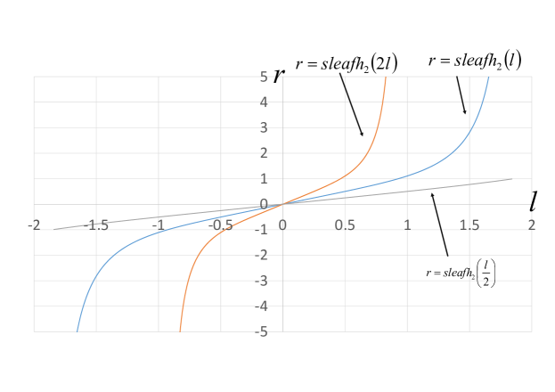
sleafh2​(2​l)=2​s​l​e​a​f​h2​(l)​1+(sleafh2​(l))41βˆ’(sleafh2​(l))4subscriptsleafh22𝑙2sleafsubscripth2𝑙1superscriptsubscriptsleafh2𝑙41superscriptsubscriptsleafh2𝑙4\mathrm{sleafh}_{2}(2l)=\frac{2\mathrm{sleafh}_{2}(l)\sqrt{1+(\mathrm{sleafh}_{2}(l))^{4}}}{1-(\mathrm{sleafh}_{2}(l))^{4}} (80)

The variables l1subscript𝑙1l_{1} and l2subscript𝑙2l_{2} in Eq. (58) and Eq. (59) are replaced with the variable l𝑙l. The double-angle formula is then defined as follows:

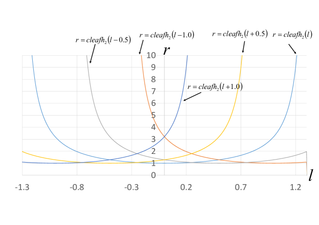
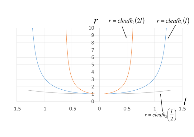
cleafh2​(2​l)=(cleafh2​(l))4+2​(cleafh2​(l))2βˆ’1βˆ’(cleafh2​(l))4+2​(cleafh2​(l))2+1subscriptcleafh22𝑙superscriptsubscriptcleafh2𝑙42superscriptsubscriptcleafh2𝑙21superscriptsubscriptcleafh2𝑙42superscriptsubscriptcleafh2𝑙21\mathrm{cleafh}_{2}(2l)=\frac{(\mathrm{cleafh}_{2}(l))^{4}+2(\mathrm{cleafh}_{2}(l))^{2}-1}{-(\mathrm{cleafh}_{2}(l))^{4}+2(\mathrm{cleafh}_{2}(l))^{2}+1} (81)

In the case where the basis n=3𝑛3n=3, the variables l1subscript𝑙1l_{1} and l2subscript𝑙2l_{2} of Eq. (62) are replaced with the variable l𝑙l, and the double-angle formula of the function sleafh3​(2​l)subscriptsleafh32𝑙\mathrm{sleafh}_{3}(2l) is defined as follows:

sleafh3​(2​l)=2​s​l​e​a​f​h3​(l)​1+(sleafh3​(l))61βˆ’8​(sleafh3​(l))6subscriptsleafh32𝑙2sleafsubscripth3𝑙1superscriptsubscriptsleafh3𝑙618superscriptsubscriptsleafh3𝑙6\mathrm{sleafh}_{3}(2l)=\frac{2\mathrm{sleafh}_{3}(l)\sqrt{1+(\mathrm{sleafh}_{3}(l))^{6}}}{\sqrt{1-8(\mathrm{sleafh}_{3}(l))^{6}}} (82)

In the case where the basis n=3𝑛3n=3, the variables l1subscript𝑙1l_{1} and l2subscript𝑙2l_{2} of Eq. (64) and Eq. (65) are replaced with the variable l𝑙l, and the double-angle formula of the function cleafh3​(2​l)subscriptcleafh32𝑙\mathrm{cleafh}_{3}(2l) is defined as follows:

cleafh3​(2​l)=2​(cleafh3​(l))2+2​(cleafh3​(l))4βˆ’11+8​(cleafh3​(l))2+8​(cleafh3​(l))6βˆ’8​(cleafh3​(l))8subscriptcleafh32𝑙2superscriptsubscriptcleafh3𝑙22superscriptsubscriptcleafh3𝑙4118superscriptsubscriptcleafh3𝑙28superscriptsubscriptcleafh3𝑙68superscriptsubscriptcleafh3𝑙8\mathrm{cleafh}_{3}(2l)=\frac{2(\mathrm{cleafh}_{3}(l))^{2}+2(\mathrm{cleafh}_{3}(l))^{4}-1}{\sqrt{1+8(\mathrm{cleafh}_{3}(l))^{2}+8(\mathrm{cleafh}_{3}(l))^{6}-8(\mathrm{cleafh}_{3}(l))^{8}}} (83)

3.4 Half Angle Formulas of Hyperbolic Leaf Functions

In the case where the basis n=2𝑛2n=2, the variables l1subscript𝑙1l_{1} and l2subscript𝑙2l_{2} in Eq. (56) are replaced with the expression l/2𝑙2l/2, and the half-angle formula is defined as follows:

(i) In the case where |l|≦΢2𝑙subscript𝜁2|l|\leqq\zeta_{2} (see Appendix F for the constant ΞΆ2subscript𝜁2\zeta_{2} and Appendix H for the periodicity n=2𝑛2n=2), the half-angle formula is expressed as follows:

(sleafh2​(l2))2=1+1+(sleafh2​(l))4(sleafh2​(l))2βˆ’2βˆ’1+1+(sleafh2​(l))4superscriptsubscriptsleafh2𝑙2211superscriptsubscriptsleafh2𝑙4superscriptsubscriptsleafh2𝑙2211superscriptsubscriptsleafh2𝑙4\Bigl{(}\mathrm{sleafh}_{2}\Bigl{(}\frac{l}{2}\Bigr{)}\Bigr{)}^{2}=\frac{1+\sqrt{1+(\mathrm{sleafh}_{2}(l))^{4}}}{(\mathrm{sleafh}_{2}(l))^{2}}-\frac{\sqrt{2}}{\sqrt{-1+\sqrt{1+(\mathrm{sleafh}_{2}(l))^{4}}}} (84)

(ii) In the case where ΞΆ2≦|l|subscript𝜁2𝑙\zeta_{2}\leqq|l|, the half-angle formula is defined as follows:

(sleafh2​(l2))2=1+1+(sleafh2​(l))4(sleafh2​(l))2+2βˆ’1+1+(sleafh2​(l))4superscriptsubscriptsleafh2𝑙2211superscriptsubscriptsleafh2𝑙4superscriptsubscriptsleafh2𝑙2211superscriptsubscriptsleafh2𝑙4\Bigl{(}\mathrm{sleafh}_{2}\Bigl{(}\frac{l}{2}\Bigr{)}\Bigr{)}^{2}=\frac{1+\sqrt{1+(\mathrm{sleafh}_{2}(l))^{4}}}{(\mathrm{sleafh}_{2}(l))^{2}}+\frac{\sqrt{2}}{\sqrt{-1+\sqrt{1+(\mathrm{sleafh}_{2}(l))^{4}}}} (85)

In the case where the basis n=2𝑛2n=2, the variables l1subscript𝑙1l_{1} and l2subscript𝑙2l_{2} in Eq. (58) and Eq. (59) are replaced with the expression l/2𝑙2l/2, and the half-angle formula can be expressed as follows (see Appendix G for the constant Ξ·2subscriptπœ‚2\eta_{2} and Appendix H for the periodicity n=2𝑛2n=2):

(i) In the case where |l|≦η2𝑙subscriptπœ‚2|l|\leqq\eta_{2}, the half-angle formula is defined as follows:

(cleafh2​(l2))2=βˆ’1+cleafh2​(l)+2​1+(cleafh2​(l))21+cleafh2​(l)superscriptsubscriptcleafh2𝑙221subscriptcleafh2𝑙21superscriptsubscriptcleafh2𝑙21subscriptcleafh2𝑙\Bigl{(}\mathrm{cleafh}_{2}\Bigl{(}\frac{l}{2}\Bigr{)}\Bigr{)}^{2}=\frac{-1+\mathrm{cleafh}_{2}(l)+\sqrt{2}\sqrt{1+(\mathrm{cleafh}_{2}(l))^{2}}}{1+\mathrm{cleafh}_{2}(l)} (86)

(ii) In the case where Ξ·2≦|l|subscriptπœ‚2𝑙\eta_{2}\leqq|l|, the half-angle formula is defined as follows:

(cleafh2​(l2))2=βˆ’1+cleafh2​(l)βˆ’2​1+(cleafh2​(l))21+cleafh2​(l)superscriptsubscriptcleafh2𝑙221subscriptcleafh2𝑙21superscriptsubscriptcleafh2𝑙21subscriptcleafh2𝑙\Bigl{(}\mathrm{cleafh}_{2}\Bigl{(}\frac{l}{2}\Bigr{)}\Bigr{)}^{2}=\frac{-1+\mathrm{cleafh}_{2}(l)-\sqrt{2}\sqrt{1+(\mathrm{cleafh}_{2}(l))^{2}}}{1+\mathrm{cleafh}_{2}(l)} (87)

In the case where the basis n=3𝑛3n=3, the variables l1subscript𝑙1l_{1} and l2subscript𝑙2l_{2} in Eq. (62) are replaced with the expression l/2𝑙2l/2, and the half-angle formula of the function sleafh3​(l)subscriptsleafh3𝑙\mathrm{sleafh}_{3}(l) is defined as follows:

(sleafh3​(l2))2=βˆ’12​(sleafh3​(l))2βˆ’12​1βˆ’(sleafh3​(l))2+(sleafh3​(l))4+12β€‹βˆ’1+(sleafh3​(l))2+2​(sleafh3​(l))4+2+2​(sleafh3​(l))61βˆ’(sleafh3​(l))2+(sleafh3​(l))4superscriptsubscriptsleafh3𝑙2212superscriptsubscriptsleafh3𝑙2121superscriptsubscriptsleafh3𝑙2superscriptsubscriptsleafh3𝑙4121superscriptsubscriptsleafh3𝑙22superscriptsubscriptsleafh3𝑙422superscriptsubscriptsleafh3𝑙61superscriptsubscriptsleafh3𝑙2superscriptsubscriptsleafh3𝑙4\begin{split}&\Bigl{(}\mathrm{sleafh}_{3}\Bigl{(}\frac{l}{2}\Bigr{)}\Bigr{)}^{2}=-\frac{1}{2}(\mathrm{sleafh}_{3}(l))^{2}-\frac{1}{2}\sqrt{1-(\mathrm{sleafh}_{3}(l))^{2}+(\mathrm{sleafh}_{3}(l))^{4}}\\ &+\frac{1}{2}\sqrt{-1+(\mathrm{sleafh}_{3}(l))^{2}+2(\mathrm{sleafh}_{3}(l))^{4}+\frac{2+2(\mathrm{sleafh}_{3}(l))^{6}}{\sqrt{1-(\mathrm{sleafh}_{3}(l))^{2}+(\mathrm{sleafh}_{3}(l))^{4}}}}\end{split} (88)

In the case where the basis n=3𝑛3n=3, the variables l1subscript𝑙1l_{1} and l2subscript𝑙2l_{2} in Eq. (64) and Eq. (65) are replaced with the expression l/2𝑙2l/2 and the half-angle formula of the function cleafh3​(l)subscriptcleafh3𝑙\mathrm{cleafh}_{3}(l) is defined as follows:

(cleafh3​(l2))2=βˆ’1+cleafh3(l))2+31+cleafh3(l))2+(cleafh3(l))44​(cleafh3​(l))2+2+3​cleafh3​(l)β€‹βˆ’3βˆ’6​(cleafh3​(l))2+2​3​{1+2​(cleafh3​(l))2}​1+(cleafh3​(l))2+(cleafh3​(l))42{1+2cleafh3(l))2}3/2\begin{split}&\Bigl{(}\mathrm{cleafh}_{3}\Bigl{(}\frac{l}{2}\Bigr{)}\Bigr{)}^{2}=\frac{-1+\mathrm{cleafh}_{3}(l))^{2}+\sqrt{3}\sqrt{1+\mathrm{cleafh}_{3}(l))^{2}+(\mathrm{cleafh}_{3}(l))^{4}}}{4(\mathrm{cleafh}_{3}(l))^{2}+2}\\ &+\frac{\sqrt{3}\mathrm{cleafh}_{3}(l)\sqrt{-3-6(\mathrm{cleafh}_{3}(l))^{2}+2\sqrt{3}\{1+2(\mathrm{cleafh}_{3}(l))^{2}\}\sqrt{1+(\mathrm{cleafh}_{3}(l))^{2}+(\mathrm{cleafh}_{3}(l))^{4}}}}{2\{1+2\mathrm{cleafh}_{3}(l))^{2}\}^{3/2}}\end{split} (89)

4 Numerical Analysis

4.1 Numerical Analysis of Leaf Functions

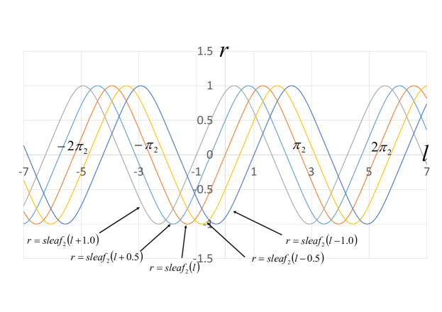
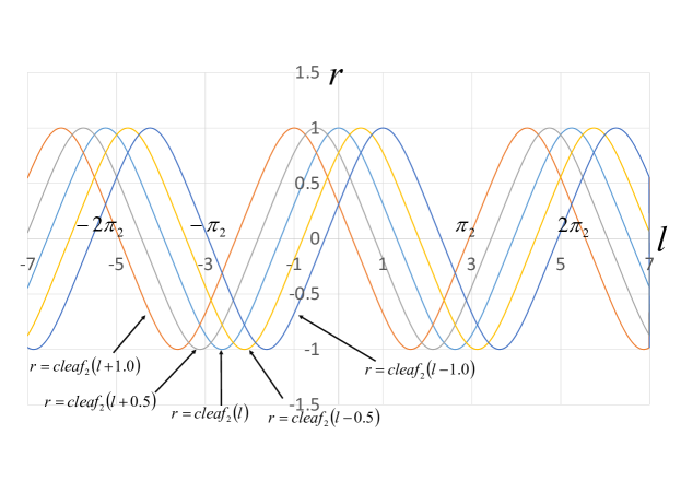
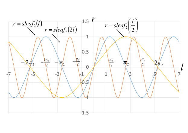
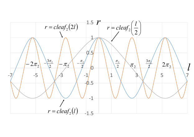
The curves of the leaf functions sleaf2​(l)subscriptsleaf2𝑙\mathrm{sleaf}_{2}(l) and cleaf2​(l)subscriptcleaf2𝑙\mathrm{cleaf}_{2}(l) are shown in Figs. 4 and 5. Numerical data for these two leaf functions are summarized in Table 1. These curves are the same curves as those of the lemniscate elliptic functions r=sl​(l)π‘Ÿsl𝑙r=\mathrm{sl}(l) and r=cl​(l)π‘Ÿcl𝑙r=\mathrm{cl}(l). Using the addition formulas of Eq. (38) ∼similar-to\sim Eq. (46), the curves of the leaf functions sleaf2​(l)subscriptsleaf2𝑙\mathrm{sleaf}_{2}(l) and cleaf2​(l)subscriptcleaf2𝑙\mathrm{cleaf}_{2}(l) are translated in the direction of the axis l𝑙l. Fig. 6 shows graphs of the double-angle sleaf2​(2​l)subscriptsleaf22𝑙\mathrm{sleaf}_{2}(2l) and the half-angle sleaf2​(l/2)subscriptsleaf2𝑙2\mathrm{sleaf}_{2}(l/2) obtained using Eqs. (67) ∼similar-to\sim (68) and Eqs. (74) ∼similar-to\sim (75) . Fig. 7 shows graphs of the double-angle cleaf2​(2​l)subscriptcleaf22𝑙\mathrm{cleaf}_{2}(2l) and the half-angle cleaf2​(l/2)subscriptcleaf2𝑙2\mathrm{cleaf}_{2}(l/2) obtained using Eqs. (69) and (76). The amplitude of the wave is 1 and one period of the function cleaf2​(l)subscriptcleaf2𝑙\mathrm{cleaf}_{2}(l) is 2​π2(=2Γ—2.622​⋯)annotated2subscriptπœ‹2absent22.622β‹―2\pi_{2}(=2\times 2.622\cdots).

As shown in Fig. 4, curves sleaf2​(l)subscriptsleaf2𝑙\mathrm{sleaf}_{2}(l) are translated using only the addition theorem, so that the period remains constant at 2​π22subscriptπœ‹22\pi_{2}. On the contrary, as shown in Fig. 6, the period changes to Ο€2subscriptπœ‹2\pi_{2} and 4​π24subscriptπœ‹24\pi_{2}, when the phase becomes 2​l2𝑙2l and l/2𝑙2l/2, respectively. Similarly, as shown in Fig. 5, curves cleaf2​(l)subscriptcleaf2𝑙\mathrm{cleaf}_{2}(l) are translated using only the addition theorem, so that the period remains constant at 2​π22subscriptπœ‹22\pi_{2}. On the contrary, as shown in Fig. 7, the period changes to Ο€2subscriptπœ‹2\pi_{2} and 4​π24subscriptπœ‹24\pi_{2}, when the phase becomes 2​l2𝑙2l and l/2𝑙2l/2, respectively. Additionally, the leaf function can be expressed as the following trigonometric function:

sleafn​(l+Ο€n2)=cleafn​(l)​(n=1,2,3,β‹―)subscriptsleaf𝑛𝑙subscriptπœ‹π‘›2subscriptcleaf𝑛𝑙𝑛123β‹―\mathrm{sleaf}_{n}\Bigl{(}l+\frac{\pi_{n}}{2}\Bigr{)}=\mathrm{cleaf}_{n}(l)\>(n=1,2,3,\cdots) (90)

Using the Eq. (90) and with constant Ο€22subscriptπœ‹22\frac{\pi_{2}}{2}, the waves are translated in the direction l𝑙l. The curve shown in the Fig. 6 represents the wave translated in the positive direction l𝑙l, as shown in the Fig. 7. Similarly, the curve shown in the Fig. 4 represents the wave translated in the positive direction l𝑙l, as shown in the Fig. 5.

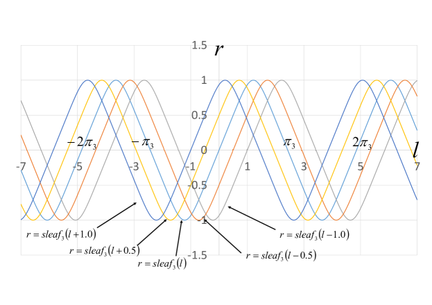
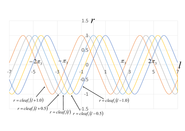
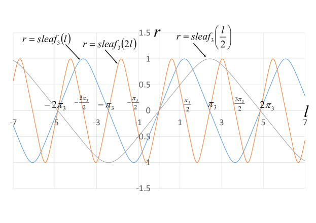
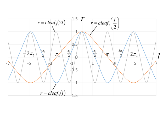
Next, the graph of the leaf function with the basis n=3𝑛3n=3 is shown. The curves of the leaf functions sleaf3​(l)subscriptsleaf3𝑙\mathrm{sleaf}_{3}(l) and cleaf3​(l)subscriptcleaf3𝑙\mathrm{cleaf}_{3}(l) are shown in Figs. 8 and 9. The horizontal and vertical axes represent the variables l𝑙l and rπ‘Ÿr, respectively. The numerical data of the leaf functions sleaf3​(l)subscriptsleaf3𝑙\mathrm{sleaf}_{3}(l) and cleaf3​(l)subscriptcleaf3𝑙\mathrm{cleaf}_{3}(l) are summarized in Table 1. The curves of the leaf functions sleaf3​(l)subscriptsleaf3𝑙\mathrm{sleaf}_{3}(l) and cleaf3​(l)subscriptcleaf3𝑙\mathrm{cleaf}_{3}(l) are translated in the direction of the axis l𝑙l. These curves of the leaf functions were obtained using the addition formulas of Eqs. (48) - (49) and Eqs. (51) - (52). Fig. 10 shows graphs of the double-angle sleaf3​(2​l)subscriptsleaf32𝑙\mathrm{sleaf}_{3}(2l) and the half-angle sleaf3​(l/2)subscriptsleaf3𝑙2\mathrm{sleaf}_{3}(l/2) obtained using Eqs. (71) ∼similar-to\sim (72) and Eqs. (77) ∼similar-to\sim (78). Fig. 11 shows graphs of the double-angle cleaf3​(2​l)subscriptcleaf32𝑙\mathrm{cleaf}_{3}(2l) and the half-angle cleaf3​(l/2)subscriptcleaf3𝑙2\mathrm{cleaf}_{3}(l/2) obtained using Eq. (73) and (79). The amplitude of the wave is 1 and one period of the function cleaf3​(l)subscriptcleaf3𝑙\mathrm{cleaf}_{3}(l) is 2​π3(=2Γ—2.429​⋯)annotated2subscriptπœ‹3absent22.429β‹―2\pi_{3}(=2\times 2.429\cdots).

When the phase is doubled, the period is halved, and vice-versa. Even with a change in the phase, the amplitude remains constant at 111, and initial condition cleaf3​(0)=1subscriptcleaf301\mathrm{cleaf}_{3}(0)=1 is maintained at l=0𝑙0l=0, as confirmed from the graph.

Refer to caption
Figure 4: Translation of the curves of the function sleaf2​(l)subscriptsleaf2𝑙\mathrm{sleaf}_{2}(l) obtained using the addition formulas with the basis n=2𝑛2n=2
Refer to caption
Figure 5: Translation of the curves of the function cleaf2​(l)subscriptcleaf2𝑙\mathrm{cleaf}_{2}(l) obtained using the addition formulas with the basis n=2𝑛2n=2
Refer to caption
Figure 6: Translation of the curves of the functions sleaf2​(l)subscriptsleaf2𝑙\mathrm{sleaf}_{2}(l), sleaf2​(2​l)subscriptsleaf22𝑙\mathrm{sleaf}_{2}(2l), and sleaf2​(l/2)subscriptsleaf2𝑙2\mathrm{sleaf}_{2}(l/2) obtained using the addition formulas based on the basis n=2𝑛2n=2
Refer to caption
Figure 7: Translation of the curves of the functions cleaf2​(l)subscriptcleaf2𝑙\mathrm{cleaf}_{2}(l), cleaf2​(2​l)subscriptcleaf22𝑙\mathrm{cleaf}_{2}(2l), and cleaf2​(l/2)subscriptcleaf2𝑙2\mathrm{cleaf}_{2}(l/2) obtained using the addition formulas based on the basis n=2𝑛2n=2
Refer to caption
Figure 8: Translation of the curves of the function sleaf3​(l)subscriptsleaf3𝑙\mathrm{sleaf}_{3}(l) obtained using the addition formulas with the basis n=3𝑛3n=3
Refer to caption
Figure 9: Translation of the curves of the function cleaf3​(l)subscriptcleaf3𝑙\mathrm{cleaf}_{3}(l) obtained using the addition formulas with the basis n=3𝑛3n=3
Refer to caption
Figure 10: Translation of the curves of the functions sleaf3​(l)subscriptsleaf3𝑙\mathrm{sleaf}_{3}(l), sleaf3​(2​l)subscriptsleaf32𝑙\mathrm{sleaf}_{3}(2l), and sleaf3​(l/2)subscriptsleaf3𝑙2\mathrm{sleaf}_{3}(l/2) obtained using the addition formulas based on the basis n=3𝑛3n=3
Refer to caption
Figure 11: Translation of the curves of the functions cleaf3​(l)subscriptcleaf3𝑙\mathrm{cleaf}_{3}(l), cleaf3​(2​l)subscriptcleaf32𝑙\mathrm{cleaf}_{3}(2l), and cleaf3​(l/2)subscriptcleaf3𝑙2\mathrm{cleaf}_{3}(l/2) obtained using the addition formulas with the basis n=3𝑛3n=3

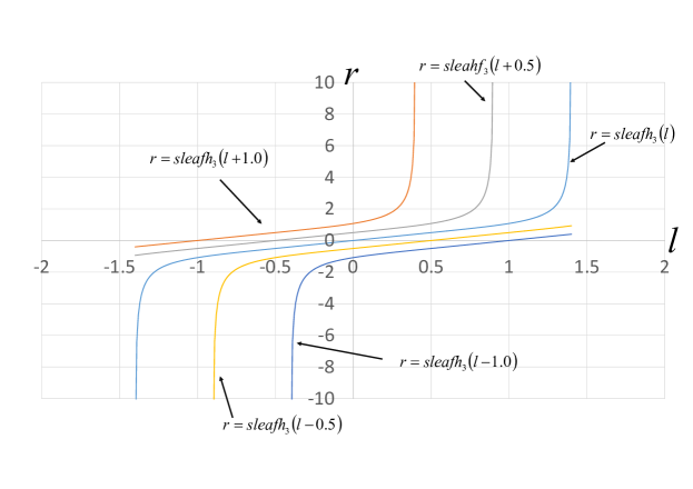
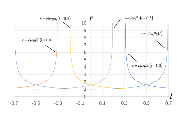
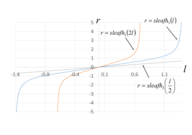
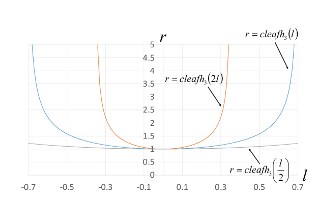
4.2 Numerical Analysis of Hyperbolic Leaf Functions

The curves of the leaf functions sleafh2​(l)subscriptsleafh2𝑙\mathrm{sleafh}_{2}(l) and cleafh2​(l)subscriptcleafh2𝑙\mathrm{cleafh}_{2}(l) are shown in Figs. 12 and 13. The horizontal and vertical axes represent the variables l𝑙l and rπ‘Ÿr. The numerical data for the leaf functions sleafh2​(l)subscriptsleafh2𝑙\mathrm{sleafh}_{2}(l) and cleafh2​(l)subscriptcleafh2𝑙\mathrm{cleafh}_{2}(l) are summarized in Table 2. Using the addition formulas of Eq. (56) and the Eqs. (58) ∼similar-to\sim (59), the curves of the leaf functions sleafh2​(l)subscriptsleafh2𝑙\mathrm{sleafh}_{2}(l) and cleafh2​(l)subscriptcleafh2𝑙\mathrm{cleafh}_{2}(l) are translated in the direction l𝑙l. Fig. 14 shows graphs of the double-angle sleafh2​(2​l)subscriptsleafh22𝑙\mathrm{sleafh}_{2}(2l) and the half-angle sleafh2​(l/2)subscriptsleafh2𝑙2\mathrm{sleafh}_{2}(l/2) obtained using Eq. (80) and Eqs. (84) ∼similar-to\sim (85) . Fig. 15 shows graphs of the double-angle cleafh2​(2​l)subscriptcleafh22𝑙\mathrm{cleafh}_{2}(2l) and the half-angle cleafh2​(l/2)subscriptcleafh2𝑙2\mathrm{cleafh}_{2}(l/2) obtained using Eq. (81) and Eqs. (86) ∼similar-to\sim (87). Limits exist for the functions sleafh2​(l)subscriptsleafh2𝑙\mathrm{sleafh}_{2}(l) and cleafh2​(l)subscriptcleafh2𝑙\mathrm{cleafh}_{2}(l), respectively (see Appendix F and Appendix G). Next, curves of the leaf functions sleafh3​(l)subscriptsleafh3𝑙\mathrm{sleafh}_{3}(l) and cleafh3​(l)subscriptcleafh3𝑙\mathrm{cleafh}_{3}(l) are shown in Figs. 16 and 17. The horizontal and vertical axes represent the variables l𝑙l and rπ‘Ÿr, respectively. The numerical data of the leaf functions sleafh3​(l)subscriptsleafh3𝑙\mathrm{sleafh}_{3}(l) and cleafh3​(l)subscriptcleafh3𝑙\mathrm{cleafh}_{3}(l) are summarized in Table 2. Using the addition formulas of Eq. (62) and Eqs. (64) ∼similar-to\sim (65), the curves of the leaf functions sleafh3​(l)subscriptsleafh3𝑙\mathrm{sleafh}_{3}(l) and cleafh3​(l)subscriptcleafh3𝑙\mathrm{cleafh}_{3}(l) are translated in the direction l𝑙l. Fig. 18 shows graphs of the double-angle sleafh3​(2​l)subscriptsleafh32𝑙\mathrm{sleafh}_{3}(2l) and the half-angle sleafh3​(l/2)subscriptsleafh3𝑙2\mathrm{sleafh}_{3}(l/2) obtained using Eq. (82) and Eq. (88).

Fig. 19 shows graphs of the double-angle cleafh3​(2​l)subscriptcleafh32𝑙\mathrm{cleafh}_{3}(2l) and the half-angle cleafh3​(l/2)subscriptcleafh3𝑙2\mathrm{cleafh}_{3}(l/2) obtained using Eqs (83) and (89). Limits exist in the functions sleafh3​(l)subscriptsleafh3𝑙\mathrm{sleafh}_{3}(l) and cleafh3​(l)subscriptcleafh3𝑙\mathrm{cleafh}_{3}(l), respectively. For the function sleafh3​(l)subscriptsleafh3𝑙\mathrm{sleafh}_{3}(l), the limit exists at Β±ΞΆ3plus-or-minussubscript𝜁3\pm\zeta_{3} (see Appendix F for the constant ΞΆ3subscript𝜁3\zeta_{3}). The curve of the function sleafh3​(l)subscriptsleafh3𝑙\mathrm{sleafh}_{3}(l) monotonically increases in the domain βˆ’ΞΆ3<l<ΞΆ3subscript𝜁3𝑙subscript𝜁3-\zeta_{3}<l<\zeta_{3}. In the case of the function cleafh3​(l)subscriptcleafh3𝑙\mathrm{cleafh}_{3}(l), the limit exists at Β±Ξ·3plus-or-minussubscriptπœ‚3\pm\eta_{3} (see Appendix G for the constant Ξ·3subscriptπœ‚3\eta_{3}). The domain of the function cleafh3​(l)subscriptcleafh3𝑙\mathrm{cleafh}_{3}(l) is βˆ’Ξ·3<l<Ξ·3subscriptπœ‚3𝑙subscriptπœ‚3-\eta_{3}<l<\eta_{3}.

Refer to caption
Figure 12: Translation of the curves of the function sleafh2​(l)subscriptsleafh2𝑙\mathrm{sleafh}_{2}(l) obtained using the addition formulas with the basis n=2𝑛2n=2
Refer to caption
Figure 13: Translation of the curves of the function cleafh2​(l)subscriptcleafh2𝑙\mathrm{cleafh}_{2}(l) obtained using the addition formulas with the basis n=2𝑛2n=2
Refer to caption
Figure 14: Translation of the curves of the functions sleafh2​(l)subscriptsleafh2𝑙\mathrm{sleafh}_{2}(l), sleafh2​(2​l)subscriptsleafh22𝑙\mathrm{sleafh}_{2}(2l) and sleafh2​(l/2)subscriptsleafh2𝑙2\mathrm{sleafh}_{2}(l/2) obtained using the addition formulas with the basis n=2𝑛2n=2
Refer to caption
Figure 15: Translation of the curves of the functions cleafh2​(l)subscriptcleafh2𝑙\mathrm{cleafh}_{2}(l), cleafh2​(2​l)subscriptcleafh22𝑙\mathrm{cleafh}_{2}(2l), and cleafh2​(l/2)subscriptcleafh2𝑙2\mathrm{cleafh}_{2}(l/2) obtained using the addition formulas with the basis n=2𝑛2n=2
Refer to caption
Figure 16: Translation of the curves of the function sleafh3​(l)subscriptsleafh3𝑙\mathrm{sleafh}_{3}(l) obtained using the addition formulas with the basis n=3𝑛3n=3
Refer to caption
Figure 17: Translation of the curves of the functions cleafh3​(l)subscriptcleafh3𝑙\mathrm{cleafh}_{3}(l) obtained using the addition formulas with the basis n=3𝑛3n=3
Refer to caption
Figure 18: Translation of the curves of the functions sleafh3​(l)subscriptsleafh3𝑙\mathrm{sleafh}_{3}(l), sleafh3​(2​l)subscriptsleafh32𝑙\mathrm{sleafh}_{3}(2l), and sleafh3​(l/2)subscriptsleafh3𝑙2\mathrm{sleafh}_{3}(l/2) obtained using the addition formulas with the basis n=3𝑛3n=3
Refer to caption
Figure 19: Translation of the curves of the functions cleafh3​(l)subscriptcleafh3𝑙\mathrm{cleafh}_{3}(l), cleafh3​(2​l)subscriptcleafh32𝑙\mathrm{cleafh}_{3}(2l), and cleafh3​(l/2)subscriptcleafh3𝑙2\mathrm{cleafh}_{3}(l/2) obtained using the addition formulas with the basis n=3𝑛3n=3

5 Conclusion

Based on the analogy between the trigonometric and hyperbolic function, the hyperbolic leaf function paired with the leaf function was defined. The main conclusions can be summarized as follows:

β‹…β‹…\cdot The relation equations between the leaf function and the hyperbolic leaf function were derived using imaginary numbers.

β‹…β‹…\cdot The addition formulas of the hyperbolic leaf function were derived by using addition formulas of the leaf function with the basis n=1,2,3𝑛123n=1,2,3.

β‹…β‹…\cdot For both the leaf function and hyperbolic leaf function for the basis n=1,2,3𝑛123n=1,2,3, half-angle and double-angle formulas were derived using addition formulas

As a future research topic, we will investigate whether the periodicity of the hyperbolic leaf function exists. In the case where the basis n=2𝑛2n=2, a limit exists in the hyperbolic function. By appropriately setting the initial conditions, the addition formulas for n=2𝑛2n=2 can be applied in all domains over the limit. Although the periodicity of the hyperbolic leaf function n=2𝑛2n=2 is evident, questions remain concerning the periodicity of the hyperbolic leaf function with n=3𝑛3n=3. In the case where the basis is n=3𝑛3n=3, a limit also exists for the hyperbolic leaf function. However, the addition formulas of the hyperbolic leaf function cannot be applied outside of its domain. At basis n=3𝑛3n=3, the periodicity of the hyperbolic leaf function is not observed. Another unaddressed issue is that the addition formulas of the leaf function with the basis n=4𝑛4n=4 or more are not known.

Table 1: Numerical data of the leaf functions
l𝑙l sleaf1​(l)subscriptsleaf1𝑙\mathrm{sleaf}_{1}(l) cleaf1​(l)subscriptcleaf1𝑙\mathrm{cleaf}_{1}(l) sleaf2​(l)subscriptsleaf2𝑙\mathrm{sleaf}_{2}(l) cleaf2​(l)subscriptcleaf2𝑙\mathrm{cleaf}_{2}(l) sleaf3​(l)subscriptsleaf3𝑙\mathrm{sleaf}_{3}(l) cleaf3​(l)subscriptcleaf3𝑙\mathrm{cleaf}_{3}(l)
0.0 0.000000000 1.000000000 0.000000000 1.000000000 0.000000000 1.000000000
0.1 0.099833417 0.995004165 0.099998987 0.990049602 0.099999991 0.98518434
0.2 0.198669331 0.980066578 0.199967976 0.960781145 0.199999064 0.942809514
0.3 0.295520207 0.955336489 0.299757126 0.913842132 0.299984331 0.878183695
0.4 0.389418342 0.921060994 0.398978135 0.851676083 0.39988294 0.797825011
0.5 0.479425539 0.877582562 0.496891146 0.777159391 0.499442694 0.70763201
0.6 0.564642473 0.825335615 0.592307034 0.693234267 0.598009242 0.611978813
0.7 0.644217687 0.764842187 0.683522566 0.602609146 0.694183101 0.513646507
0.8 0.717356091 0.696706709 0.768312999 0.507563306 0.785387303 0.414175714
0.9 0.78332691 0.621609968 0.844009686 0.409858439 0.867486256 0.314303714
1.0 0.841470985 0.540302306 0.90768321 0.310738001 0.934767593 0.214323891
1.1 0.89120736 0.453596121 0.956432623 0.210987025 0.980707849 0.114325366
1.2 0.932039086 0.362357754 0.987748032 0.111027204 0.999692203 0.014325392
1.3 0.963558185 0.267498829 0.999878378 0.011028912 0.989089542 -0.085674597
1.4 0.98544973 0.169967143 0.99211532 -0.088970511 0.950392842 -0.185674048
1.5 0.997494987 0.070737202 0.96491412 -0.188946955 0.888559535 -0.285663493
1.6 0.999573603 -0.029199522 0.919815574 -0.288769649 0.810063642 -0.385583945
1.7 0.99166481 -0.128844494 0.859192306 -0.388082304 0.720971617 -0.485219858
1.8 0.973847631 -0.227202095 0.785891649 -0.486189025 0.6258955 -0.583992736
1.9 0.946300088 -0.323289567 0.702864932 -0.581954203 0.527828311 -0.680635105
2.0 0.909297427 -0.416146837 0.612857981 -0.673732946 0.428461029 -0.772765772
2.1 0.863209367 -0.504846105 0.518203565 -0.759356014 0.328621294 -0.856486525
2.2 0.808496404 -0.588501117 0.420721859 -0.836196738 0.228648563 -0.92628646
2.3 0.745705212 -0.666276021 0.3217114 -0.90134206 0.128650882 -0.975673073
2.4 0.675463181 -0.737393716 0.222003575 -0.951870972 0.028650956 -0.998769949
2.5 0.598472144 -0.801143616 0.122054841 -0.985211764 -0.071349009 -0.992412076
2.6 0.515501372 -0.856888753 0.022057545 -0.999513456 -0.171348665 -0.95749878
2.7 0.42737988 -0.904072142 -0.077942171 -0.993943297 -0.2713412 -0.898594215
2.8 0.33498815 -0.942222341 -0.177924624 -0.968828424 -0.371279371 -0.822087294
2.9 0.239249329 -0.970958165 -0.277776677 -0.925599649 -0.470980082 -0.734191026
3.0 0.141120008 -0.989992497 -0.37717265 -0.866554268 -0.569933963 -0.639752776
Table 2: Numerical data of the hyperbolic leaf functions
l𝑙l sleafh1​(l)subscriptsleafh1𝑙\mathrm{sleafh}_{1}(l) cleafh1​(l)subscriptcleafh1𝑙\mathrm{cleafh}_{1}(l) sleafh2​(l)subscriptsleafh2𝑙\mathrm{sleafh}_{2}(l) cleafh2​(l)subscriptcleafh2𝑙\mathrm{cleafh}_{2}(l) sleafh3​(l)subscriptsleafh3𝑙\mathrm{sleafh}_{3}(l) cleafh3​(l)subscriptcleafh3𝑙\mathrm{cleafh}_{3}(l)
0.0 0.000000000 1.000000000 0.000000000 1.000000000 0.000000000 1.000000000
0.1 0.10016675 1.005004168 0.100001013 1.010050409 0.100000009 1.015190873
0.2 0.201336003 1.020066756 0.200032033 1.040819784 0.200000936 1.063219846
0.3 0.304520293 1.045338514 0.300243205 1.094280966 0.300015671 1.152957367
0.4 0.410752326 1.081072372 0.401026247 1.174155432 0.400117152 1.306327433
0.5 0.521095305 1.127625965 0.503141445 1.286737533 0.500558986 1.583264962
0.6 0.636653582 1.185465218 0.607861028 1.442514133 0.6020087 2.225120045
0.7 0.758583702 1.255169006 0.717150413 1.659450947 0.705950043 21.4096535
0.8 0.888105982 1.337434946 0.833926854 1.97019847 0.815368602 βˆ’-
0.9 1.026516726 1.433086385 0.962467567 2.439868366 0.936017909 βˆ’-
1.0 1.175201194 1.543080635 1.10910404 3.218148246 1.079143503 βˆ’-
1.1 1.33564747 1.668518554 1.283479658 4.739635312 1.26866512 βˆ’-
1.2 1.509461355 1.810655567 1.500980956 9.006830737 1.566095647 βˆ’-
1.3 1.698382437 1.97091423 1.787828613 90.67397241 2.210887381 βˆ’-
1.4 1.904301501 2.150898465 2.192926988 βˆ’- 15.13849028 βˆ’-
Table 3: Values of constants Ο€nsubscriptπœ‹π‘›\pi_{n}
n𝑛n Ο€nsubscriptπœ‹π‘›\pi_{n}
1 3.1415 β‹―β‹―\cdots
2 2.6220 β‹―β‹―\cdots
3 2.4286 β‹―β‹―\cdots
β‹―β‹―\cdots β‹―β‹―\cdots
Table 4: Limits ΞΆnsubscriptπœπ‘›\zeta_{n} of the hyperbolic leaf function sleafhn​(l)subscriptsleafh𝑛𝑙\mathrm{sleafh}_{n}(l)
n𝑛n ΞΆnsubscriptπœπ‘›\zeta_{n}
1 Not applicable β‹―β‹―\cdots
2 1.8540 β‹―β‹―\cdots
3 1.4021 β‹―β‹―\cdots
β‹―β‹―\cdots β‹―β‹―\cdots
Table 5: Limits Ξ·nsubscriptπœ‚π‘›\eta_{n} of the hyperbolic leaf function cleafhn​(l)subscriptcleafh𝑛𝑙\mathrm{cleafh}_{n}(l)
n𝑛n Ξ·nsubscriptπœ‚π‘›\eta_{n}
1 Not applicable β‹―β‹―\cdots
2 1.31102 β‹―β‹―\cdots
3 0.70109 β‹―β‹―\cdots
β‹―β‹―\cdots β‹―β‹―\cdots

Appendix Appendix A

The relation equations with the basis n=1𝑛1n=1 are described. The relation equation between the leaf function sleaf1​(l)subscriptsleaf1𝑙\mathrm{sleaf}_{1}(l) and the leaf function cleaf1​(l)subscriptcleaf1𝑙\mathrm{cleaf}_{1}(l) is as follows:

(sleaf1​(l))2+(cleaf1​(l))2=1superscriptsubscriptsleaf1𝑙2superscriptsubscriptcleaf1𝑙21(\mathrm{sleaf}_{1}(l))^{2}+(\mathrm{cleaf}_{1}(l))^{2}=1 (91)

The relation equation between the hyperbolic leaf function sleafh1​(l)subscriptsleafh1𝑙\mathrm{sleafh}_{1}(l) and the hyperbolic leaf function cleafh1​(l)subscriptcleafh1𝑙\mathrm{cleafh}_{1}(l) is as follows:

(cleafh1​(l))2βˆ’(sleafh1​(l))2=1superscriptsubscriptcleafh1𝑙2superscriptsubscriptsleafh1𝑙21(\mathrm{cleafh}_{1}(l))^{2}-(\mathrm{sleafh}_{1}(l))^{2}=1 (92)

Appendix Appendix B

The relation equations with the basis n=2𝑛2n=2 are described. The relation equation between the leaf function sleaf2​(l)subscriptsleaf2𝑙\mathrm{sleaf}_{2}(l) and the leaf function cleaf2​(l)subscriptcleaf2𝑙\mathrm{cleaf}_{2}(l) is as follows[1]:

(sleaf2​(l))2+(cleaf2​(l))2+(sleaf2​(l))2β‹…(cleaf2​(l))2=1superscriptsubscriptsleaf2𝑙2superscriptsubscriptcleaf2𝑙2β‹…superscriptsubscriptsleaf2𝑙2superscriptsubscriptcleaf2𝑙21(\mathrm{sleaf}_{2}(l))^{2}+(\mathrm{cleaf}_{2}(l))^{2}+(\mathrm{sleaf}_{2}(l))^{2}\cdot(\mathrm{cleaf}_{2}(l))^{2}=1 (93)

The relation equation between the hyperbolic leaf function sleafh2​(l)subscriptsleafh2𝑙\mathrm{sleafh}_{2}(l) and the hyperbolic leaf function cleafh2​(l)subscriptcleafh2𝑙\mathrm{cleafh}_{2}(l) is as follows[33, 32]:

cleafh2​(2​l)=1+(sleafh2​(l))21βˆ’(sleafh2​(l))2subscriptcleafh22𝑙1superscriptsubscriptsleafh2𝑙21superscriptsubscriptsleafh2𝑙2\mathrm{cleafh}_{2}(\sqrt{2}l)=\frac{1+(\mathrm{sleafh}_{2}(l))^{2}}{1-(\mathrm{sleafh}_{2}(l))^{2}} (94)

The relation equation between the hyperbolic leaf function cleaf2​(l)subscriptcleaf2𝑙\mathrm{cleaf}_{2}(l) and the hyperbolic leaf function cleafh2​(l)subscriptcleafh2𝑙\mathrm{cleafh}_{2}(l) is as follows:

cleaf2​(l)β‹…cleafh2​(l)=1β‹…subscriptcleaf2𝑙subscriptcleafh2𝑙1\mathrm{cleaf}_{2}(l)\cdot\mathrm{cleafh}_{2}(l)=1 (95)

The relation equation between the hyperbolic leaf function sleaf2​(l)subscriptsleaf2𝑙\mathrm{sleaf}_{2}(l) and the hyperbolic leaf function sleafh2​(l)subscriptsleafh2𝑙\mathrm{sleafh}_{2}(l) is as follows:

(sleaf2​(2​l))2=2​(sleafh2​(l))21+(sleafh2​(l))4superscriptsubscriptsleaf22𝑙22superscriptsubscriptsleafh2𝑙21superscriptsubscriptsleafh2𝑙4(\mathrm{sleaf}_{2}(\sqrt{2}l))^{2}=\frac{2(\mathrm{sleafh}_{2}(l))^{2}}{1+(\mathrm{sleafh}_{2}(l))^{4}} (96)

Appendix Appendix C

The relation equations with the basis n=3𝑛3n=3 are described. The relation equation between the leaf functions sleaf3​(l)subscriptsleaf3𝑙\mathrm{sleaf}_{3}(l) and cleaf3​(l)subscriptcleaf3𝑙\mathrm{cleaf}_{3}(l) is as follows [1]:

(sleaf3​(l))2+(cleaf3​(l))2+2​(sleaf3​(l))2β‹…(cleaf3​(l))2=1superscriptsubscriptsleaf3𝑙2superscriptsubscriptcleaf3𝑙2β‹…2superscriptsubscriptsleaf3𝑙2superscriptsubscriptcleaf3𝑙21(\mathrm{sleaf}_{3}(l))^{2}+(\mathrm{cleaf}_{3}(l))^{2}+2(\mathrm{sleaf}_{3}(l))^{2}\cdot(\mathrm{cleaf}_{3}(l))^{2}=1 (97)

The relation equation between the hyperbolic leaf functions sleafh3​(l)subscriptsleafh3𝑙\mathrm{sleafh}_{3}(l) and cleafh3​(l)subscriptcleafh3𝑙\mathrm{cleafh}_{3}(l) is as follows[33, 32]:

(cleafh3​(l))2βˆ’(sleafh3​(l))2βˆ’2​(sleafh3​(l))2β‹…(cleafh3​(l))2=1superscriptsubscriptcleafh3𝑙2superscriptsubscriptsleafh3𝑙2β‹…2superscriptsubscriptsleafh3𝑙2superscriptsubscriptcleafh3𝑙21(\mathrm{cleafh}_{3}(l))^{2}-(\mathrm{sleafh}_{3}(l))^{2}-2(\mathrm{sleafh}_{3}(l))^{2}\cdot(\mathrm{cleafh}_{3}(l))^{2}=1 (98)

Appendix Appendix D

Using the imaginary number, the relations between the leaf function and hyperbolic leaf function are described in the works[33, 32]. To derive the relation between these two functions, the following equation is defined:

r=iβ‹…uπ‘Ÿβ‹…π‘–π‘’r=i\cdot u (99)

The symbol i𝑖i represents the imaginary number. Substituting the preceding equation yields the following:

l=∫0iβ‹…ud​t1βˆ’t2​n(=arcsleafn​(iβ‹…u))𝑙annotatedsuperscriptsubscript0⋅𝑖𝑒d𝑑1superscript𝑑2𝑛absentsubscriptarcsleaf𝑛⋅𝑖𝑒l=\int_{0}^{i\cdot u}\frac{\mathrm{d}t}{\sqrt{1-t^{2n}}}(=\mathrm{arcsleaf}_{n}(i\cdot u)) (100)

Here, the parameter t𝑑t is replaced with iβ‹…ΞΎβ‹…π‘–πœ‰i\cdot\xi (t=iβ‹…ΞΎπ‘‘β‹…π‘–πœ‰t=i\cdot\xi). In the case where t=0𝑑0t=0, ΞΎπœ‰\xi is zero. In the case where t=iβ‹…u𝑑⋅𝑖𝑒t=i\cdot u, ΞΎπœ‰\xi is u𝑒u. Thus, the following equation is obtained:

l=∫0uiβ‹…d​ξ1βˆ’(iβ‹…ΞΎ)2​n=iβ‹…βˆ«0ud​ξ1βˆ’i2​nβ‹…ΞΎ2​n𝑙superscriptsubscript0𝑒⋅𝑖dπœ‰1superscriptβ‹…π‘–πœ‰2𝑛⋅𝑖superscriptsubscript0𝑒dπœ‰1β‹…superscript𝑖2𝑛superscriptπœ‰2𝑛l=\int_{0}^{u}\frac{i\cdot\mathrm{d}\xi}{\sqrt{1-(i\cdot\xi)^{2n}}}=i\cdot\int_{0}^{u}\frac{\mathrm{d}\xi}{\sqrt{1-i^{2n}\cdot\xi^{2n}}} (101)

Let n𝑛n be an odd number, that is, n=2​mβˆ’1​(m=1,2,3,β‹―)𝑛2π‘š1π‘š123β‹―n=2m-1(m=1,2,3,\cdots). The following equation is then obtained:

l=iβ‹…βˆ«0ud​ξ1βˆ’i2​nβ‹…ΞΎ2​n=iβ‹…βˆ«0ud​ξ1+ΞΎ2​n=iβ‹…asleafhn​(u)𝑙⋅𝑖superscriptsubscript0𝑒dπœ‰1β‹…superscript𝑖2𝑛superscriptπœ‰2𝑛⋅𝑖superscriptsubscript0𝑒dπœ‰1superscriptπœ‰2𝑛⋅𝑖subscriptasleafh𝑛𝑒l=i\cdot\int_{0}^{u}\frac{\mathrm{d}\xi}{\sqrt{1-i^{2n}\cdot\xi^{2n}}}=i\cdot\int_{0}^{u}\frac{\mathrm{d}\xi}{\sqrt{1+\xi^{2n}}}=i\cdot\mathrm{asleafh}_{n}(u) (102)

The following equation is obtained based on the preceding equation as follows:

sleafhn​(li)=usubscriptsleafh𝑛𝑙𝑖𝑒\mathrm{sleafh}_{n}\Bigl{(}\frac{l}{i}\Bigr{)}=u (103)
sleafhn​(βˆ’iβ‹…l)=usubscriptsleafh𝑛⋅𝑖𝑙𝑒\mathrm{sleafh}_{n}(-i\cdot l)=u (104)

Here, the leaf function sleafhn​(l)subscriptsleafh𝑛𝑙\mathrm{sleafh}_{n}(l) has the following relation[33]:

sleafhn​(βˆ’l)=βˆ’sleafhn​(l)subscriptsleafh𝑛𝑙subscriptsleafh𝑛𝑙\mathrm{sleafh}_{n}(-l)=-\mathrm{sleafh}_{n}(l) (105)

Eq. (103) can be transformed as follows:

βˆ’sleafhn​(iβ‹…l)=usubscriptsleafh𝑛⋅𝑖𝑙𝑒-\mathrm{sleafh}_{n}(i\cdot l)=u (106)

The following equation is obtained using Eq. (100) and Eq. (106):

sleafn​(l)=βˆ’iβ‹…sleafhn​(iβ‹…l)subscriptsleaf𝑛𝑙⋅𝑖subscriptsleafh𝑛⋅𝑖𝑙\mathrm{sleaf}_{n}(l)=-i\cdot\mathrm{sleafh}_{n}(i\cdot l) (107)

Next, let us consider the case where n𝑛n is an even number. In the case where n=2​m​(m=1,2,3​⋯)𝑛2π‘šπ‘š123β‹―n=2m(m=1,2,3\cdots), the following equation is obtained:

l=iβ‹…βˆ«0ud​ξ1βˆ’i2​nβ‹…ΞΎ2​n=iβ‹…βˆ«0ud​ξ1βˆ’ΞΎ2​n=iβ‹…arcsleafn​(u)𝑙⋅𝑖superscriptsubscript0𝑒dπœ‰1β‹…superscript𝑖2𝑛superscriptπœ‰2𝑛⋅𝑖superscriptsubscript0𝑒dπœ‰1superscriptπœ‰2𝑛⋅𝑖subscriptarcsleaf𝑛𝑒l=i\cdot\int_{0}^{u}\frac{\mathrm{d}\xi}{\sqrt{1-i^{2n}\cdot\xi^{2n}}}=i\cdot\int_{0}^{u}\frac{\mathrm{d}\xi}{\sqrt{1-\xi^{2n}}}=i\cdot\mathrm{arcsleaf}_{n}(u) (108)

The following equation is obtained:

sleafn​(li)=usubscriptsleaf𝑛𝑙𝑖𝑒\mathrm{sleaf}_{n}\Bigl{(}\frac{l}{i}\Bigr{)}=u (109)
sleafn​(βˆ’iβ‹…l)=usubscriptsleaf𝑛⋅𝑖𝑙𝑒\mathrm{sleaf}_{n}(-i\cdot l)=u (110)

Here, the leaf function sleafn​(l)subscriptsleaf𝑛𝑙\mathrm{sleaf}_{n}(l) has the following relation[2]:

sleafn​(βˆ’l)=βˆ’sleafn​(l)subscriptsleaf𝑛𝑙subscriptsleaf𝑛𝑙\mathrm{sleaf}_{n}(-l)=-\mathrm{sleaf}_{n}(l) (111)

Eq. (110) can be expressed as follows:

βˆ’sleafn​(iβ‹…l)=usubscriptsleaf𝑛⋅𝑖𝑙𝑒-\mathrm{sleaf}_{n}(i\cdot l)=u (112)

The following equation is obtained using Eq. (100) and Eq. (112):

sleafn​(l)=βˆ’iβ‹…sleafn​(iβ‹…l)subscriptsleaf𝑛𝑙⋅𝑖subscriptsleaf𝑛⋅𝑖𝑙\mathrm{sleaf}_{n}(l)=-i\cdot\mathrm{sleaf}_{n}(i\cdot l) (113)

In the case where n𝑛n is an even number, the following equation is also derived:

sleafhn​(l)=βˆ’iβ‹…sleafhn​(iβ‹…l)subscriptsleafh𝑛𝑙⋅𝑖subscriptsleafh𝑛⋅𝑖𝑙\mathrm{sleafh}_{n}(l)=-i\cdot\mathrm{sleafh}_{n}(i\cdot l) (114)

Next, the equation can be transformed as follows:

l=∫1rd​tt2​nβˆ’1=∫1rd​ti​1βˆ’t2​n=1iβ‹…βˆ«1rd​t1βˆ’t2​n=1i​arccleafn​(r)𝑙superscriptsubscript1π‘Ÿd𝑑superscript𝑑2𝑛1superscriptsubscript1π‘Ÿd𝑑𝑖1superscript𝑑2𝑛⋅1𝑖superscriptsubscript1π‘Ÿd𝑑1superscript𝑑2𝑛1𝑖subscriptarccleafπ‘›π‘Ÿl=\int_{1}^{r}\frac{\mathrm{d}t}{\sqrt{t^{2n}-1}}=\int_{1}^{r}\frac{\mathrm{d}t}{i\sqrt{1-t^{2n}}}=\frac{1}{i}\cdot\int_{1}^{r}\frac{\mathrm{d}t}{\sqrt{1-t^{2n}}}=\frac{1}{i}\mathrm{arccleaf}_{n}(r) (115)

The following equation is obtained by the Eq. (115):

r=cleafn​(iβ‹…l)π‘Ÿsubscriptcleaf𝑛⋅𝑖𝑙r=\mathrm{cleaf}_{n}(i\cdot l) (116)

The following equation is also obtained by the Eq. (115):

r=cleafhn​(l)π‘Ÿsubscriptcleafh𝑛𝑙r=\mathrm{cleafh}_{n}(l) (117)

The following equation is obtained using Eq. (116) and Eq. (117):

cleafn​(iβ‹…l)=cleafhn​(l)subscriptcleaf𝑛⋅𝑖𝑙subscriptcleafh𝑛𝑙\mathrm{cleaf}_{n}(i\cdot l)=\mathrm{cleafh}_{n}(l) (118)

Alternatively, the following equation is obtained by substituting iβ‹…l⋅𝑖𝑙i\cdot l into l𝑙l:

cleafn​(l)=cleafhn​(iβ‹…l)subscriptcleaf𝑛𝑙subscriptcleafh𝑛⋅𝑖𝑙\mathrm{cleaf}_{n}(l)=\mathrm{cleafh}_{n}(i\cdot l) (119)

In the preceding equation, the following equation is applied:

cleafn​(l)=cleafn​(βˆ’l)subscriptcleaf𝑛𝑙subscriptcleaf𝑛𝑙\mathrm{cleaf}_{n}(l)=\mathrm{cleaf}_{n}(-l) (120)

Appendix Appendix E

The constants Ο€nsubscriptπœ‹π‘›\pi_{n} are defined as follows[2, 1]:

Ο€n=2β€‹βˆ«0111βˆ’t2​n​dt​(n=1,2,3​⋯)subscriptπœ‹π‘›2superscriptsubscript0111superscript𝑑2𝑛differential-d𝑑𝑛123β‹―\pi_{n}=2\int_{0}^{1}\frac{1}{\sqrt{1-t^{2n}}}\mathrm{d}t(n=1,2,3\cdots) (121)

In the case where n=1𝑛1n=1, the constant Ο€1subscriptπœ‹1\pi_{1} represents the circular constant Ο€πœ‹\pi. The constants Ο€n​(n=1,2,3​⋯)subscriptπœ‹π‘›π‘›123β‹―\pi_{n}(n=1,2,3\cdots) are summarized in Table 3.

Appendix Appendix F

Except for the basis n=1𝑛1n=1, the limit of the variable l𝑙l exists in the hyperbolic leaf function sleafhn​(l)subscriptsleafh𝑛𝑙\mathrm{sleafh}_{n}(l)[33]. The limit with the basis n𝑛n is defined as ΞΆnsubscriptπœπ‘›\zeta_{n}. The limit ΞΆnsubscriptπœπ‘›\zeta_{n} is obtained by the following equation:

ΞΆn=∫0∞11+t2​n​dt​(n=2,3​⋯)subscriptπœπ‘›superscriptsubscript011superscript𝑑2𝑛differential-d𝑑𝑛23β‹―\zeta_{n}=\int_{0}^{\infty}\frac{1}{\sqrt{1+t^{2n}}}\mathrm{d}t(n=2,3\cdots) (122)

The constants ΞΆn​(n=2,3​⋯)subscriptπœπ‘›π‘›23β‹―\zeta_{n}(n=2,3\cdots) are summarized in Table 4.

Appendix Appendix G

Except for the basis n=1𝑛1n=1, the limit of the variable l𝑙l exists in the hyperbolic leaf function cleafhn​(l)subscriptcleafh𝑛𝑙\mathrm{cleafh}_{n}(l)[32]. The limit with the basis n𝑛n is defined as Ξ·nsubscriptπœ‚π‘›\eta_{n}. The limit Ξ·nsubscriptπœ‚π‘›\eta_{n} is obtained using the following equation:

Ξ·n=∫1∞1t2​nβˆ’1​dt​(n=2,3​⋯)subscriptπœ‚π‘›superscriptsubscript11superscript𝑑2𝑛1differential-d𝑑𝑛23β‹―\eta_{n}=\int_{1}^{\infty}\frac{1}{\sqrt{t^{2n}-1}}\mathrm{d}t(n=2,3\cdots) (123)

The constants Ξ·n​(n=2,3​⋯)subscriptπœ‚π‘›π‘›23β‹―\eta_{n}(n=2,3\cdots) are summarized in Table 5.

Appendix Appendix H

The function sleafhn​(l)subscriptsleafh𝑛𝑙\mathrm{sleafh}_{n}(l) and cleafhn​(l)subscriptcleafh𝑛𝑙\mathrm{cleafh}_{n}(l) have limits. The domains of the variable l𝑙l are defined as Eq. (8) and Eq. (12), respectively. Therefore, the values of the hyperbolic leaf function cannot be defined under the domain |l|>ΞΆn𝑙subscriptπœπ‘›|l|>\zeta_{n} in the function sleafhn​(l)subscriptsleafh𝑛𝑙\mathrm{sleafh}_{n}(l) or |l|>Ξ·n𝑙subscriptπœ‚π‘›|l|>\eta_{n} in the function cleafhn​(l)subscriptcleafh𝑛𝑙\mathrm{cleafh}_{n}(l). In the case where n=1𝑛1n=1, the limits do not exist in the hyperbolic leaf function as sleafh1​(l)subscriptsleafh1𝑙\mathrm{sleafh}_{1}(l) and cleafh1​(l)subscriptcleafh1𝑙\mathrm{cleafh}_{1}(l) represent sinh​(l)sinh𝑙\mathrm{sinh}(l) and cosh​(l)cosh𝑙\mathrm{cosh}(l), respectively. In the case where n=2𝑛2n=2 (sleafh2​(l)subscriptsleafh2𝑙\mathrm{sleafh}_{2}(l) and cleafh2​(l)subscriptcleafh2𝑙\mathrm{cleafh}_{2}(l)), the initial values of the variables r​(0)π‘Ÿ0r(0) and d​r​(0)/d​tπ‘‘π‘Ÿ0𝑑𝑑dr(0)/dt are defined by Eqs. (9) and (10), or Eq. (13) and (14). The initial values in the function sleafh2​(l)subscriptsleafh2𝑙\mathrm{sleafh}_{2}(l) are redefined as follows:

r​(2​m​΢2)=sleafh2​(2​m​΢2)=0π‘Ÿ2π‘šsubscript𝜁2subscriptsleafh22π‘šsubscript𝜁20r(2m\zeta_{2})=\mathrm{sleafh}_{2}(2m\zeta_{2})=0 (124)
d​r​(2​m​΢2)d​l=dd​l​sleafh2​(2​m​΢2)=1dπ‘Ÿ2π‘šsubscript𝜁2d𝑙dd𝑙subscriptsleafh22π‘šsubscript𝜁21\frac{\mathrm{d}r(2m\zeta_{2})}{\mathrm{d}l}=\frac{\mathrm{d}}{\mathrm{d}l}\mathrm{sleafh}_{2}(2m\zeta_{2})=1 (125)

The initial values of the function cleafh2​(l)subscriptcleafh2𝑙\mathrm{cleafh}_{2}(l) are redefined as follows:

r​(4​m​η2)=cleafh2​(4​m​η2)=1π‘Ÿ4π‘šsubscriptπœ‚2subscriptcleafh24π‘šsubscriptπœ‚21r(4m\eta_{2})=\mathrm{cleafh}_{2}(4m\eta_{2})=1 (126)
r​((4​mβˆ’2)​η2)=cleafh2​((4​mβˆ’2)​η2)=βˆ’1π‘Ÿ4π‘š2subscriptπœ‚2subscriptcleafh24π‘š2subscriptπœ‚21r((4m-2)\eta_{2})=\mathrm{cleafh}_{2}((4m-2)\eta_{2})=-1 (127)
d​r​(2​m​η2)d​l=dd​l​cleafh2​(2​m​η2)=0dπ‘Ÿ2π‘šsubscriptπœ‚2d𝑙dd𝑙subscriptcleafh22π‘šsubscriptπœ‚20\frac{\mathrm{d}r(2m\eta_{2})}{\mathrm{d}l}=\frac{\mathrm{d}}{\mathrm{d}l}\mathrm{cleafh}_{2}(2m\eta_{2})=0 (128)

The variable mπ‘šm represents an integer. The graph based on these definitions is shown in Fig. 20 (sleafh2​(l)subscriptsleafh2𝑙\mathrm{sleafh}_{2}(l) ) and Fig. 21 (cleafh2​(l)subscriptcleafh2𝑙\mathrm{cleafh}_{2}(l) ), respectively. Such definitions are consistent for all the formulas such as the addition, double-angle, and half-angle formulas. These formulas work under all domains. In the case n=2𝑛2n=2, the hyperbolic leaf functions can be extended for all domains. In the case where n=3𝑛3n=3 in the hyperbolic leaf function, the addition, double-angle, and half-angle formulas do not work in the domain |l|>ΞΆ3𝑙subscript𝜁3|l|>\zeta_{3} of |l|>Ξ·3𝑙subscriptπœ‚3|l|>\eta_{3}, even if the initial conditions are defined by equations such as r​(2​m​΢3)=sleafh3​(2​m​΢3)=0π‘Ÿ2π‘šsubscript𝜁3subscriptsleafh32π‘šsubscript𝜁30r(2m\zeta_{3})=\mathrm{sleafh}_{3}(2m\zeta_{3})=0. In the case where n≧3𝑛3n\geqq 3, the values of sleafhn​(l)subscriptsleafh𝑛𝑙\mathrm{sleafh}_{n}(l) and cleafhnsubscriptcleafh𝑛\mathrm{cleafh}_{n} are unknown for the domain |l|>ΞΆn𝑙subscriptπœπ‘›|l|>\zeta_{n} of |l|>Ξ·n𝑙subscriptπœ‚π‘›|l|>\eta_{n}.

Refer to caption
Figure 20: Curves of the extended hyperbolic leaf function sleafh2​(l)subscriptsleafh2𝑙\mathrm{sleafh}_{2}(l) for the initial conditions: Eq. (124) and Eq. (125)
Refer to caption
Figure 21: Curves of the extended hyperbolic leaf function cleafh2​(l)subscriptcleafh2𝑙\mathrm{cleafh}_{2}(l) for the initial conditions: Eq. (126), Eq. (127), and Eq. (128)

Appendix Appendix I

Eq. (47) is set as follows:

{g​(l1,l2)}2={p1​(l1,l2)}2p3​(l1,l2)+{p2​(l1,l2)}2p3​(l1,l2)superscript𝑔subscript𝑙1subscript𝑙22superscriptsubscript𝑝1subscript𝑙1subscript𝑙22subscript𝑝3subscript𝑙1subscript𝑙2superscriptsubscript𝑝2subscript𝑙1subscript𝑙22subscript𝑝3subscript𝑙1subscript𝑙2\{g(l_{1},l_{2})\}^{2}=\frac{\{p_{1}(l_{1},l_{2})\}^{2}}{p_{3}(l_{1},l_{2})}+\frac{\{p_{2}(l_{1},l_{2})\}^{2}}{p_{3}(l_{1},l_{2})} (129)
g​(l1,l2)=sleaf3​(l1+l2)𝑔subscript𝑙1subscript𝑙2subscriptsleaf3subscript𝑙1subscript𝑙2g(l_{1},l_{2})=\mathrm{sleaf}_{3}(l_{1}+l_{2}) (130)
p1​(l1,l2)=sleaf3​(l1)β€‹βˆ‚sleaf3​(l2)βˆ‚l2+sleaf3​(l2)β€‹βˆ‚sleaf3​(l1)βˆ‚l1subscript𝑝1subscript𝑙1subscript𝑙2subscriptsleaf3subscript𝑙1subscriptsleaf3subscript𝑙2subscript𝑙2subscriptsleaf3subscript𝑙2subscriptsleaf3subscript𝑙1subscript𝑙1p_{1}(l_{1},l_{2})=\mathrm{sleaf}_{3}(l_{1})\frac{\partial\mathrm{sleaf}_{3}(l_{2})}{\partial l_{2}}+\mathrm{sleaf}_{3}(l_{2})\frac{\partial\mathrm{sleaf}_{3}(l_{1})}{\partial l_{1}} (131)
p2​(l1,l2)=(sleaf3​(l1))3​sleaf3​(l2)βˆ’sleaf3​(l1)​(sleaf3​(l2))3subscript𝑝2subscript𝑙1subscript𝑙2superscriptsubscriptsleaf3subscript𝑙13subscriptsleaf3subscript𝑙2subscriptsleaf3subscript𝑙1superscriptsubscriptsleaf3subscript𝑙23p_{2}(l_{1},l_{2})=(\mathrm{sleaf}_{3}(l_{1}))^{3}\mathrm{sleaf}_{3}(l_{2})-\mathrm{sleaf}_{3}(l_{1})(\mathrm{sleaf}_{3}(l_{2}))^{3} (132)
p3​(l1,l2)=1+4​(sleaf3​(l1))4​(sleaf3​(l2))2+4​(sleaf3​(l1))2​(sleaf3​(l2))4subscript𝑝3subscript𝑙1subscript𝑙214superscriptsubscriptsleaf3subscript𝑙14superscriptsubscriptsleaf3subscript𝑙224superscriptsubscriptsleaf3subscript𝑙12superscriptsubscriptsleaf3subscript𝑙24p_{3}(l_{1},l_{2})=1+4(\mathrm{sleaf}_{3}(l_{1}))^{4}(\mathrm{sleaf}_{3}(l_{2}))^{2}+4(\mathrm{sleaf}_{3}(l_{1}))^{2}(\mathrm{sleaf}_{3}(l_{2}))^{4} (133)

The following equations are obtained by differentiating with respect to variablel1subscript𝑙1l_{1}:

βˆ‚p1​(l1,l2)βˆ‚l1=βˆ‚sleaf3​(l1)βˆ‚l1β€‹βˆ‚sleaf3​(l2)βˆ‚l2βˆ’3​s​l​e​a​f3​(l2)​(sleaf3​(l1))5subscript𝑝1subscript𝑙1subscript𝑙2subscript𝑙1subscriptsleaf3subscript𝑙1subscript𝑙1subscriptsleaf3subscript𝑙2subscript𝑙23sleasubscriptf3subscript𝑙2superscriptsubscriptsleaf3subscript𝑙15\frac{\partial p_{1}(l_{1},l_{2})}{\partial l_{1}}=\frac{\partial\mathrm{sleaf}_{3}(l_{1})}{\partial l_{1}}\frac{\partial\mathrm{sleaf}_{3}(l_{2})}{\partial l_{2}}-3\mathrm{sleaf}_{3}(l_{2})(\mathrm{sleaf}_{3}(l_{1}))^{5} (134)
βˆ‚p2​(l1,l2)βˆ‚l1=3​(sleaf3​(l1))2​sleaf3​(l2)β€‹βˆ‚sleaf3​(l1)βˆ‚l1βˆ’(sleaf3​(l2))3β€‹βˆ‚sleaf3​(l1)βˆ‚l1subscript𝑝2subscript𝑙1subscript𝑙2subscript𝑙13superscriptsubscriptsleaf3subscript𝑙12subscriptsleaf3subscript𝑙2subscriptsleaf3subscript𝑙1subscript𝑙1superscriptsubscriptsleaf3subscript𝑙23subscriptsleaf3subscript𝑙1subscript𝑙1\frac{\partial p_{2}(l_{1},l_{2})}{\partial l_{1}}=3(\mathrm{sleaf}_{3}(l_{1}))^{2}\mathrm{sleaf}_{3}(l_{2})\frac{\partial\mathrm{sleaf}_{3}(l_{1})}{\partial l_{1}}-(\mathrm{sleaf}_{3}(l_{2}))^{3}\frac{\partial\mathrm{sleaf}_{3}(l_{1})}{\partial l_{1}} (135)
βˆ‚p3​(l1,l2)βˆ‚l1=16​(sleaf3​(l1))3​(sleaf3​(l2))2β€‹βˆ‚sleaf3​(l1)βˆ‚l1+8​s​l​e​a​f3​(l1)​(sleaf3​(l2))4β€‹βˆ‚sleaf3​(l1)βˆ‚l1subscript𝑝3subscript𝑙1subscript𝑙2subscript𝑙116superscriptsubscriptsleaf3subscript𝑙13superscriptsubscriptsleaf3subscript𝑙22subscriptsleaf3subscript𝑙1subscript𝑙18sleasubscriptf3subscript𝑙1superscriptsubscriptsleaf3subscript𝑙24subscriptsleaf3subscript𝑙1subscript𝑙1\frac{\partial p_{3}(l_{1},l_{2})}{\partial l_{1}}=16(\mathrm{sleaf}_{3}(l_{1}))^{3}(\mathrm{sleaf}_{3}(l_{2}))^{2}\frac{\partial\mathrm{sleaf}_{3}(l_{1})}{\partial l_{1}}+8\mathrm{sleaf}_{3}(l_{1})(\mathrm{sleaf}_{3}(l_{2}))^{4}\frac{\partial\mathrm{sleaf}_{3}(l_{1})}{\partial l_{1}} (136)

The following equations are obtained by differentiating with respect to variable l2subscript𝑙2l_{2}:

βˆ‚p1​(l1,l2)βˆ‚l2=βˆ‚sleaf3​(l1)βˆ‚l1β€‹βˆ‚sleaf3​(l2)βˆ‚l2βˆ’3​s​l​e​a​f3​(l1)​(sleaf3​(l2))5subscript𝑝1subscript𝑙1subscript𝑙2subscript𝑙2subscriptsleaf3subscript𝑙1subscript𝑙1subscriptsleaf3subscript𝑙2subscript𝑙23sleasubscriptf3subscript𝑙1superscriptsubscriptsleaf3subscript𝑙25\frac{\partial p_{1}(l_{1},l_{2})}{\partial l_{2}}=\frac{\partial\mathrm{sleaf}_{3}(l_{1})}{\partial l_{1}}\frac{\partial\mathrm{sleaf}_{3}(l_{2})}{\partial l_{2}}-3\mathrm{sleaf}_{3}(l_{1})(\mathrm{sleaf}_{3}(l_{2}))^{5} (137)
βˆ‚p2​(l1,l2)βˆ‚l2=βˆ’3​(sleaf3​(l2))2​sleaf3​(l1)β€‹βˆ‚sleaf3​(l2)βˆ‚l2+(sleaf3​(l1))3β€‹βˆ‚sleaf3​(l2)βˆ‚l2subscript𝑝2subscript𝑙1subscript𝑙2subscript𝑙23superscriptsubscriptsleaf3subscript𝑙22subscriptsleaf3subscript𝑙1subscriptsleaf3subscript𝑙2subscript𝑙2superscriptsubscriptsleaf3subscript𝑙13subscriptsleaf3subscript𝑙2subscript𝑙2\frac{\partial p_{2}(l_{1},l_{2})}{\partial l_{2}}=-3(\mathrm{sleaf}_{3}(l_{2}))^{2}\mathrm{sleaf}_{3}(l_{1})\frac{\partial\mathrm{sleaf}_{3}(l_{2})}{\partial l_{2}}+(\mathrm{sleaf}_{3}(l_{1}))^{3}\frac{\partial\mathrm{sleaf}_{3}(l_{2})}{\partial l_{2}} (138)
βˆ‚p3​(l1,l2)βˆ‚l2=16​(sleaf3​(l2))3​(sleaf3​(l1))2β€‹βˆ‚sleaf3​(l2)βˆ‚l2+8​s​l​e​a​f3​(l2)​(sleaf3​(l1))4β€‹βˆ‚sleaf3​(l2)βˆ‚l2subscript𝑝3subscript𝑙1subscript𝑙2subscript𝑙216superscriptsubscriptsleaf3subscript𝑙23superscriptsubscriptsleaf3subscript𝑙12subscriptsleaf3subscript𝑙2subscript𝑙28sleasubscriptf3subscript𝑙2superscriptsubscriptsleaf3subscript𝑙14subscriptsleaf3subscript𝑙2subscript𝑙2\frac{\partial p_{3}(l_{1},l_{2})}{\partial l_{2}}=16(\mathrm{sleaf}_{3}(l_{2}))^{3}(\mathrm{sleaf}_{3}(l_{1}))^{2}\frac{\partial\mathrm{sleaf}_{3}(l_{2})}{\partial l_{2}}+8\mathrm{sleaf}_{3}(l_{2})(\mathrm{sleaf}_{3}(l_{1}))^{4}\frac{\partial\mathrm{sleaf}_{3}(l_{2})}{\partial l_{2}} (139)

Using Eq. (129), the following equations are obtained by differentiating with respect to variable l1subscript𝑙1l_{1}:

βˆ‚g​(l1,l2)βˆ‚l1=(2​p1​(l1,l2)β€‹βˆ‚p1​(l1,l2)βˆ‚l1+2​p2​(l1,l2)β€‹βˆ‚p2​(l1,l2)βˆ‚l1)​p3​(l1,l2)2​g​(l1,l2)​p3​(l1,l2)2βˆ’(p1​(l1,l2)2+p2​(l1,l2)2)β€‹βˆ‚p3​(l1,l2)βˆ‚l12​g​(l1,l2)​p3​(l1,l2)2𝑔subscript𝑙1subscript𝑙2subscript𝑙12subscript𝑝1subscript𝑙1subscript𝑙2subscript𝑝1subscript𝑙1subscript𝑙2subscript𝑙12subscript𝑝2subscript𝑙1subscript𝑙2subscript𝑝2subscript𝑙1subscript𝑙2subscript𝑙1subscript𝑝3subscript𝑙1subscript𝑙22𝑔subscript𝑙1subscript𝑙2subscript𝑝3superscriptsubscript𝑙1subscript𝑙22subscript𝑝1superscriptsubscript𝑙1subscript𝑙22subscript𝑝2superscriptsubscript𝑙1subscript𝑙22subscript𝑝3subscript𝑙1subscript𝑙2subscript𝑙12𝑔subscript𝑙1subscript𝑙2subscript𝑝3superscriptsubscript𝑙1subscript𝑙22\begin{split}&\frac{\partial g(l_{1},l_{2})}{\partial l_{1}}=\frac{\Big{(}2p_{1}(l_{1},l_{2})\frac{\partial p_{1}(l_{1},l_{2})}{\partial l_{1}}+2p_{2}(l_{1},l_{2})\frac{\partial p_{2}(l_{1},l_{2})}{\partial l_{1}}\Big{)}p_{3}(l_{1},l_{2})}{2g(l_{1},l_{2})p_{3}(l_{1},l_{2})^{2}}\\ &-\frac{\Big{(}p_{1}(l_{1},l_{2})^{2}+p_{2}(l_{1},l_{2})^{2}\Big{)}\frac{\partial p_{3}(l_{1},l_{2})}{\partial l_{1}}}{2g(l_{1},l_{2})p_{3}(l_{1},l_{2})^{2}}\end{split} (140)

Using Eqs. (134) ∼similar-to\sim (136), the numerator in the Eq. (140) is expanded as:

(2​p1​(l1,l2)β€‹βˆ‚p1​(l1,l2)βˆ‚l1+2​p2​(l1,l2)β€‹βˆ‚p2​(l1,l2)βˆ‚l1)​p3​(l1,l2)βˆ’(p1​(l1,l2)2+p2​(l1,l2)2)β€‹βˆ‚p3​(l1,l2)βˆ‚l1=(2sleaf3(l1)βˆ’8(sleaf3(l1))5(sleaf3(l2))2βˆ’24(sleaf3(l1))3(sleaf3(l2))4βˆ’8sleaf3(l1)(sleaf3(l2))6βˆ’16(sleaf3(l1))5(sleaf3(l2))8)βˆ‚sleaf3​(l1)βˆ‚l1+(2sleaf3(l2)βˆ’8(sleaf3(l1))5(sleaf3(l2))2βˆ’24(sleaf3(l1))4(sleaf3(l2))3βˆ’8(sleaf3(l1))6sleaf3(l2)βˆ’16(sleaf3(l1))8(sleaf3(l2))5)βˆ‚sleaf3​(l2)βˆ‚l22subscript𝑝1subscript𝑙1subscript𝑙2subscript𝑝1subscript𝑙1subscript𝑙2subscript𝑙12subscript𝑝2subscript𝑙1subscript𝑙2subscript𝑝2subscript𝑙1subscript𝑙2subscript𝑙1subscript𝑝3subscript𝑙1subscript𝑙2subscript𝑝1superscriptsubscript𝑙1subscript𝑙22subscript𝑝2superscriptsubscript𝑙1subscript𝑙22subscript𝑝3subscript𝑙1subscript𝑙2subscript𝑙12sleasubscriptf3subscript𝑙18superscriptsubscriptsleaf3subscript𝑙15superscriptsubscriptsleaf3subscript𝑙2224superscriptsubscriptsleaf3subscript𝑙13superscriptsubscriptsleaf3subscript𝑙248sleasubscriptf3subscript𝑙1superscriptsubscriptsleaf3subscript𝑙2616superscriptsubscriptsleaf3subscript𝑙15superscriptsubscriptsleaf3subscript𝑙28subscriptsleaf3subscript𝑙1subscript𝑙12sleasubscriptf3subscript𝑙28superscriptsubscriptsleaf3subscript𝑙15superscriptsubscriptsleaf3subscript𝑙2224superscriptsubscriptsleaf3subscript𝑙14superscriptsubscriptsleaf3subscript𝑙238superscriptsubscriptsleaf3subscript𝑙16subscriptsleaf3subscript𝑙216superscriptsubscriptsleaf3subscript𝑙18superscriptsubscriptsleaf3subscript𝑙25subscriptsleaf3subscript𝑙2subscript𝑙2\begin{split}&\Big{(}2p_{1}(l_{1},l_{2})\frac{\partial p_{1}(l_{1},l_{2})}{\partial l_{1}}+2p_{2}(l_{1},l_{2})\frac{\partial p_{2}(l_{1},l_{2})}{\partial l_{1}}\Big{)}p_{3}(l_{1},l_{2})\\ &-\Big{(}p_{1}(l_{1},l_{2})^{2}+p_{2}(l_{1},l_{2})^{2}\Big{)}\frac{\partial p_{3}(l_{1},l_{2})}{\partial l_{1}}\\ &=\Big{(}2\mathrm{sleaf}_{3}(l_{1})-8(\mathrm{sleaf}_{3}(l_{1}))^{5}(\mathrm{sleaf}_{3}(l_{2}))^{2}-24(\mathrm{sleaf}_{3}(l_{1}))^{3}(\mathrm{sleaf}_{3}(l_{2}))^{4}\\ &-8\mathrm{sleaf}_{3}(l_{1})(\mathrm{sleaf}_{3}(l_{2}))^{6}-16(\mathrm{sleaf}_{3}(l_{1}))^{5}(\mathrm{sleaf}_{3}(l_{2}))^{8}\Big{)}\frac{\partial\mathrm{sleaf}_{3}(l_{1})}{\partial l_{1}}\\ &+\Big{(}2\mathrm{sleaf}_{3}(l_{2})-8(\mathrm{sleaf}_{3}(l_{1}))^{5}(\mathrm{sleaf}_{3}(l_{2}))^{2}-24(\mathrm{sleaf}_{3}(l_{1}))^{4}(\mathrm{sleaf}_{3}(l_{2}))^{3}\\ &-8(\mathrm{sleaf}_{3}(l_{1}))^{6}\mathrm{sleaf}_{3}(l_{2})-16(\mathrm{sleaf}_{3}(l_{1}))^{8}(\mathrm{sleaf}_{3}(l_{2}))^{5}\Big{)}\frac{\partial\mathrm{sleaf}_{3}(l_{2})}{\partial l_{2}}\\ \end{split} (141)

Usingthe Eq. (129), the following equation is obtained by differentiating with respect to the variable l2subscript𝑙2l_{2}:

βˆ‚g​(l1,l2)βˆ‚l2=(2​p1​(l1,l2)β€‹βˆ‚p1​(l1,l2)βˆ‚l2+2​p2​(l1,l2)β€‹βˆ‚p2​(l1,l2)βˆ‚l2)​p3​(l1,l2)2​g​(l1,l2)​p3​(l1,l2)2βˆ’(p1​(l1,l2)2+p2​(l1,l2)2)β€‹βˆ‚p3​(l1,l2)βˆ‚l22​g​(l1,l2)​p3​(l1,l2)2𝑔subscript𝑙1subscript𝑙2subscript𝑙22subscript𝑝1subscript𝑙1subscript𝑙2subscript𝑝1subscript𝑙1subscript𝑙2subscript𝑙22subscript𝑝2subscript𝑙1subscript𝑙2subscript𝑝2subscript𝑙1subscript𝑙2subscript𝑙2subscript𝑝3subscript𝑙1subscript𝑙22𝑔subscript𝑙1subscript𝑙2subscript𝑝3superscriptsubscript𝑙1subscript𝑙22subscript𝑝1superscriptsubscript𝑙1subscript𝑙22subscript𝑝2superscriptsubscript𝑙1subscript𝑙22subscript𝑝3subscript𝑙1subscript𝑙2subscript𝑙22𝑔subscript𝑙1subscript𝑙2subscript𝑝3superscriptsubscript𝑙1subscript𝑙22\begin{split}&\frac{\partial g(l_{1},l_{2})}{\partial l_{2}}=\frac{\Big{(}2p_{1}(l_{1},l_{2})\frac{\partial p_{1}(l_{1},l_{2})}{\partial l_{2}}+2p_{2}(l_{1},l_{2})\frac{\partial p_{2}(l_{1},l_{2})}{\partial l_{2}}\Big{)}p_{3}(l_{1},l_{2})}{2g(l_{1},l_{2})p_{3}(l_{1},l_{2})^{2}}\\ &-\frac{\Big{(}p_{1}(l_{1},l_{2})^{2}+p_{2}(l_{1},l_{2})^{2}\Big{)}\frac{\partial p_{3}(l_{1},l_{2})}{\partial l_{2}}}{2g(l_{1},l_{2})p_{3}(l_{1},l_{2})^{2}}\end{split} (142)

Using Eqs. (137) ∼similar-to\sim (139), the numerator in the Eq. (142) is expanded to obtain the following relation:

βˆ‚g​(l1,l2)βˆ‚l1=βˆ‚g​(l1,l2)βˆ‚l2𝑔subscript𝑙1subscript𝑙2subscript𝑙1𝑔subscript𝑙1subscript𝑙2subscript𝑙2\frac{\partial g(l_{1},l_{2})}{\partial l_{1}}=\frac{\partial g(l_{1},l_{2})}{\partial l_{2}} (143)

The following equation is derived from the Eq. (143) (see Appendix J).

g​(l1,l2)=g​(l1+l2,0)𝑔subscript𝑙1subscript𝑙2𝑔subscript𝑙1subscript𝑙20g(l_{1},l_{2})=g(l_{1}+l_{2},0) (144)

Using the initial condition sleaf3​(0)=0subscriptsleaf300\mathrm{sleaf}_{3}(0)=0 and βˆ‚sleaf3​(0)βˆ‚l=1subscriptsleaf30𝑙1\frac{\partial\mathrm{sleaf}_{3}(0)}{\partial l}=1, the function g​(l1+l2,0)𝑔subscript𝑙1subscript𝑙20g(l_{1}+l_{2},0) is obtained as follows:

{g​(l1+l2,0)}2={p1​(l1+l2,0)}2p3​(l1+l2,0)+{p2​(l1+l2,0)}2p3​(l1+l2,0)=(sleaf3​(l1+l2))2superscript𝑔subscript𝑙1subscript𝑙202superscriptsubscript𝑝1subscript𝑙1subscript𝑙202subscript𝑝3subscript𝑙1subscript𝑙20superscriptsubscript𝑝2subscript𝑙1subscript𝑙202subscript𝑝3subscript𝑙1subscript𝑙20superscriptsubscriptsleaf3subscript𝑙1subscript𝑙22\{g(l_{1}+l_{2},0)\}^{2}=\frac{\{p_{1}(l_{1}+l_{2},0)\}^{2}}{p_{3}(l_{1}+l_{2},0)}+\frac{\{p_{2}(l_{1}+l_{2},0)\}^{2}}{p_{3}(l_{1}+l_{2},0)}=(\mathrm{sleaf}_{3}(l_{1}+l_{2}))^{2} (145)

Using Eqs. (129), (144) and (145), the following equation is obtained.

(sleaf3​(l1+l2))2={g​(l1+l2,0)}2={g​(l1,l2)}2={sleaf3​(l1)β€‹βˆ‚sleaf3​(l2)βˆ‚l2+sleaf3​(l2)β€‹βˆ‚sleaf3​(l1)βˆ‚l1}21+4​(sleaf3​(l1))4​(sleaf3​(l2))2+4​(sleaf3​(l1))2​(sleaf3​(l2))4+{(sleaf3​(l1))3​sleaf3​(l2)βˆ’sleaf3​(l1)​(sleaf3​(l2))3}21+4​(sleaf3​(l1))4​(sleaf3​(l2))2+4​(sleaf3​(l1))2​(sleaf3​(l2))4superscriptsubscriptsleaf3subscript𝑙1subscript𝑙22superscript𝑔subscript𝑙1subscript𝑙202superscript𝑔subscript𝑙1subscript𝑙22superscriptsubscriptsleaf3subscript𝑙1subscriptsleaf3subscript𝑙2subscript𝑙2subscriptsleaf3subscript𝑙2subscriptsleaf3subscript𝑙1subscript𝑙1214superscriptsubscriptsleaf3subscript𝑙14superscriptsubscriptsleaf3subscript𝑙224superscriptsubscriptsleaf3subscript𝑙12superscriptsubscriptsleaf3subscript𝑙24superscriptsuperscriptsubscriptsleaf3subscript𝑙13subscriptsleaf3subscript𝑙2subscriptsleaf3subscript𝑙1superscriptsubscriptsleaf3subscript𝑙23214superscriptsubscriptsleaf3subscript𝑙14superscriptsubscriptsleaf3subscript𝑙224superscriptsubscriptsleaf3subscript𝑙12superscriptsubscriptsleaf3subscript𝑙24\begin{split}&(\mathrm{sleaf}_{3}(l_{1}+l_{2}))^{2}=\{g(l_{1}+l_{2},0)\}^{2}=\{g(l_{1},l_{2})\}^{2}\\ &=\frac{\left\{\mathrm{sleaf}_{3}(l_{1})\frac{\mathrm{\partial sleaf}_{3}(l_{2})}{\mathrm{\partial}l_{2}}+\mathrm{sleaf}_{3}(l_{2})\frac{\mathrm{\partial sleaf}_{3}(l_{1})}{\mathrm{\partial}l_{1}}\right\}^{2}}{1+4(\mathrm{sleaf}_{3}(l_{1}))^{4}(\mathrm{sleaf}_{3}(l_{2}))^{2}+4(\mathrm{sleaf}_{3}(l_{1}))^{2}(\mathrm{sleaf}_{3}(l_{2}))^{4}}\\ &+\frac{\left\{(\mathrm{sleaf}_{3}(l_{1}))^{3}\mathrm{sleaf}_{3}(l_{2})-\mathrm{sleaf}_{3}(l_{1})(\mathrm{sleaf}_{3}(l_{2}))^{3}\right\}^{2}}{1+4(\mathrm{sleaf}_{3}(l_{1}))^{4}(\mathrm{sleaf}_{3}(l_{2}))^{2}+4(\mathrm{sleaf}_{3}(l_{1}))^{2}(\mathrm{sleaf}_{3}(l_{2}))^{4}}\end{split} (146)

Appendix Appendix J

The necessary and sufficient condition to satisfy g​(l1,l2)=g​(l1+l2,0)𝑔subscript𝑙1subscript𝑙2𝑔subscript𝑙1subscript𝑙20g(l_{1},l_{2})=g(l_{1}+l_{2},0) is that βˆ‚g​(l1,l2)βˆ‚l1=βˆ‚g​(l1,l2)βˆ‚l2𝑔subscript𝑙1subscript𝑙2subscript𝑙1𝑔subscript𝑙1subscript𝑙2subscript𝑙2\frac{\partial g(l_{1},l_{2})}{\partial l_{1}}=\frac{\partial g(l_{1},l_{2})}{\partial l_{2}} holds. Function h​(x,y)β„Žπ‘₯𝑦h(x,y) is defined as follows.

h​(x,y)=g​(x+y,xβˆ’y)β„Žπ‘₯𝑦𝑔π‘₯𝑦π‘₯𝑦h(x,y)=g(x+y,x-y) (147)
l1=x+ysubscript𝑙1π‘₯𝑦l_{1}=x+y (148)
l2=xβˆ’ysubscript𝑙2π‘₯𝑦l_{2}=x-y (149)

By differentiating the Eq. (147) equation with respect to y𝑦y, the following equation is obtained.

βˆ‚h​(x,y)βˆ‚y=βˆ‚g​(x+y,xβˆ’y)βˆ‚l1β€‹βˆ‚l1βˆ‚y+βˆ‚g​(x+y,xβˆ’y)βˆ‚l2β€‹βˆ‚l2βˆ‚y=βˆ‚g​(x+y,xβˆ’y)βˆ‚l1βˆ’βˆ‚g​(x+y,xβˆ’y)βˆ‚l2β„Žπ‘₯𝑦𝑦𝑔π‘₯𝑦π‘₯𝑦subscript𝑙1subscript𝑙1𝑦𝑔π‘₯𝑦π‘₯𝑦subscript𝑙2subscript𝑙2𝑦𝑔π‘₯𝑦π‘₯𝑦subscript𝑙1𝑔π‘₯𝑦π‘₯𝑦subscript𝑙2\begin{split}&\frac{\partial h(x,y)}{\partial y}=\frac{\partial g(x+y,x-y)}{\partial l_{1}}\frac{\partial l_{1}}{\partial y}+\frac{\partial g(x+y,x-y)}{\partial l_{2}}\frac{\partial l_{2}}{\partial y}\\ &=\frac{\partial g(x+y,x-y)}{\partial l_{1}}-\frac{\partial g(x+y,x-y)}{\partial l_{2}}\end{split} (150)

Therefore, if the equation βˆ‚gβˆ‚l1=βˆ‚gβˆ‚l2𝑔subscript𝑙1𝑔subscript𝑙2\frac{\partial g}{\partial l_{1}}=\frac{\partial g}{\partial l_{2}} holds, the following equation holds.

βˆ‚h​(x,y)βˆ‚y=0β„Žπ‘₯𝑦𝑦0\frac{\partial h(x,y)}{\partial y}=0 (151)

Using the Eq. (151), we find that h​(x,y)β„Žπ‘₯𝑦h(x,y) is a function of xπ‘₯x and not of y𝑦y. Therefore, the following equation holds for any constant aπ‘Ža and b𝑏b:

h​(x,a)=h​(x,b)β„Žπ‘₯π‘Žβ„Žπ‘₯𝑏h(x,a)=h(x,b) (152)

Here, we set the following equation:

x=b=l1+l22=0π‘₯𝑏subscript𝑙1subscript𝑙220x=b=\frac{l_{1}+l_{2}}{2}=0 (153)
a=l1βˆ’l22=0π‘Žsubscript𝑙1subscript𝑙220a=\frac{l_{1}-l_{2}}{2}=0 (154)

The following equation is obtained by using the Eqs. (150), (153), and (154):

h​(x,a)=h​(l1+l22,l1βˆ’l22)=g​(l1+l22+l1βˆ’l22,l1+l22βˆ’l1βˆ’l22)=g​(l1,l2)β„Žπ‘₯π‘Žβ„Žsubscript𝑙1subscript𝑙22subscript𝑙1subscript𝑙22𝑔subscript𝑙1subscript𝑙22subscript𝑙1subscript𝑙22subscript𝑙1subscript𝑙22subscript𝑙1subscript𝑙22𝑔subscript𝑙1subscript𝑙2h(x,a)=h\Big{(}\frac{l_{1}+l_{2}}{2},\frac{l_{1}-l_{2}}{2}\Big{)}=g\Big{(}\frac{l_{1}+l_{2}}{2}+\frac{l_{1}-l_{2}}{2},\frac{l_{1}+l_{2}}{2}-\frac{l_{1}-l_{2}}{2}\Big{)}=g(l_{1},l_{2}) (155)
h​(x,b)=h​(l1+l22,l1+l22)=g​(l1+l22+l1+l22,l1+l22βˆ’l1+l22)=g​(l1+l2,0)β„Žπ‘₯π‘β„Žsubscript𝑙1subscript𝑙22subscript𝑙1subscript𝑙22𝑔subscript𝑙1subscript𝑙22subscript𝑙1subscript𝑙22subscript𝑙1subscript𝑙22subscript𝑙1subscript𝑙22𝑔subscript𝑙1subscript𝑙20h(x,b)=h\Big{(}\frac{l_{1}+l_{2}}{2},\frac{l_{1}+l_{2}}{2}\Big{)}=g\Big{(}\frac{l_{1}+l_{2}}{2}+\frac{l_{1}+l_{2}}{2},\frac{l_{1}+l_{2}}{2}-\frac{l_{1}+l_{2}}{2}\Big{)}=g(l_{1}+l_{2},0) (156)

The following equation is obtained by using the Eqs. (152), (155) and (156).

g​(l1,l2)=g​(l1+l2,0)𝑔subscript𝑙1subscript𝑙2𝑔subscript𝑙1subscript𝑙20g(l_{1},l_{2})=g(l_{1}+l_{2},0) (157)

Conversely, if the Eq. (157) holds, the following relational expression can be obtained by using Eqs. (147) and (157).

h​(x,y)=g​(x+y,xβˆ’y)=g​(2​x,0)β„Žπ‘₯𝑦𝑔π‘₯𝑦π‘₯𝑦𝑔2π‘₯0h(x,y)=g(x+y,x-y)=g(2x,0) (158)

Eq. (158) is differentiated with respect to variable y𝑦y to obtain the following equation:

βˆ‚h​(x,y)βˆ‚y=βˆ‚g​(2​x,0)βˆ‚y=0β„Žπ‘₯𝑦𝑦𝑔2π‘₯0𝑦0\frac{\partial h(x,y)}{\partial y}=\frac{\partial g(2x,0)}{\partial y}=0 (159)

Further, the following equation is obtained by using the Eq. (150).

βˆ‚g​(x+y,xβˆ’y)βˆ‚l1=βˆ‚g​(x+y,xβˆ’y)βˆ‚l2𝑔π‘₯𝑦π‘₯𝑦subscript𝑙1𝑔π‘₯𝑦π‘₯𝑦subscript𝑙2\frac{\partial g(x+y,x-y)}{\partial l_{1}}=\frac{\partial g(x+y,x-y)}{\partial l_{2}} (160)

Using the Eqs. (148) and (149), the following equation is obtained.

βˆ‚g​(l1,l2)βˆ‚l1=βˆ‚g​(l1,l2)βˆ‚l2𝑔subscript𝑙1subscript𝑙2subscript𝑙1𝑔subscript𝑙1subscript𝑙2subscript𝑙2\frac{\partial g(l_{1},l_{2})}{\partial l_{1}}=\frac{\partial g(l_{1},l_{2})}{\partial l_{2}} (161)

References

  • [1] Kazunori Shinohara. Special function: Leaf function r=c​l​e​a​fn​(l)π‘Ÿπ‘π‘™π‘’π‘Žsubscript𝑓𝑛𝑙r=cleaf_{n}(l) (second report). Bulletin of Daido University, 51:39–68, 2015.
  • [2] Kazunori Shinohara. Special function: Leaf function r=s​l​e​a​fn​(l)π‘Ÿπ‘ π‘™π‘’π‘Žsubscript𝑓𝑛𝑙r=sleaf_{n}(l) (first report). Bulletin of Daido University, 51:23–38, 2015.
  • [3] C.F. Gauss, W.C. Waterhouse, and A.A. Clarke. Disquisitiones Arithmeticae. Springer-Verlag, 1986.
  • [4] B.Β C. Carlson. Algorithms involving arithmetic and geometric means. The American Mathematical Monthly, 78(5):496–505, 1971.
  • [5] Edward Neuman. On lemniscate functions. Integral Transforms and Special Functions, 24(3):164–171, 2013.
  • [6] E.W. Weisstein. CRC Concise Encyclopedia of Mathematics, Second Edition. CRC Press, 2002.
  • [7] R.Β Roy. Elliptic and Modular Functions from Gauss to Dedekind to Hecke. Cambridge University Press, 2017.
  • [8] Raymond Ayoub. The lemniscate and fagnano’s contributions to elliptic integrals. Archive for History of Exact Sciences, 29(2):131–149, 1984.
  • [9] L.Β Euler. Leonhardi Euleri Opera omnia. Teubner, Leipzig, 1911.
  • [10] C.Β G.Β J. Jacobi. Opuscula Mathematica. Mathematische Werke. Nabu Press, 2010.
  • [11] Kazunori Shinohara. Addition formulas of leaf functions according to integral root of polynomial based on analogies of inverse trigonometric functions and inverse lemniscate functions. Applied Mathematical Sciences, 11:2561–2577, 01 2017.
  • [12] Precious Sibanda and Ahmed Khidir. A new modification of the hpm for the duffing equation with cubic nonlinearity. International Conference on Applied and Computational Mathematics, 2, 01 2011.
  • [13] Honghua Dai. A simple collocation scheme for obtaining the periodic solutions of the duf?ng equation, and its equivalence to the high dimensional harmonic balance method: Subharmonic oscillations. Computer Modeling in Engineering and Sciences, 84:459–497, 09 2012.
  • [14] Berna Bulbul. Numerical solution of duffing equation by using an improved taylor matrix method. Journal of Applied Mathematics, 2013, 06 2013.
  • [15] Alex Elias-Zuniga. Quintication method to obtain approximate analytical solutions of non-linear oscillators. Applied Mathematics and Computation, 243:849 – 855, 2014.
  • [16] Khosro Sayevand, Dumitru Baleanu, and M.Β Fardi. A perturbative analysis of nonlinear cubic-quintic duffing oscillators. Proceedings of the Romanian Academy Series A - Mathematics Physics Technical Sciences Information Science, 15:228–234, 07 2014.
  • [17] Reza Novin and Ziba Dastjerd. Solving duffing equation using an improved semi-analytical method. Communications on Advanced Computational Science with Applications, 2015:54–58, 01 2015.
  • [18] Ying Zhang, Lin Du, Xiaole Yue, Qun Han, and Tong Fang. Analysis of symmetry breaking bifurcation in duffing system with random parameter. CMES - Computer Modeling in Engineering and Sciences, 106:37–51, 05 2015.
  • [19] Svetlin Stoyanov. Analytical and numerical investigation on the duffing oscilator subjected to a polyharmonic force excitation. Journal of Theoretical and Applied Mechanics, 45, 03 2015.
  • [20] A.M. El-Naggar and G.M. Ismail. Analytical solution of strongly nonlinear duffing oscillators. Alexandria Engineering Journal, 55(2):1581 – 1585, 2016.
  • [21] Majeed Weli and Sayl Abd-Al-Razaq. A semi analytical iterative technique for solving duffing equations. International Journal of Pure and Applied Mathematics, 108:871–885, 08 2016.
  • [22] MdΒ Hosen. Solution of cubic-quintic duffing oscillators using harmonic balance method. Malaysian Journal of Mathematical Sciences, 10:181–192, 02 2016.
  • [23] M.S.H. Chowdhury, Md.Β Alal Hosen, Kartini Ahmad, M.Y. Ali, and A.F. Ismail. High-order approximate solutions of strongly nonlinear cubic-quintic duffing oscillator based on the harmonic balance method. Results in Physics, 7:3962 – 3967, 2017.
  • [24] Mustafa Karahan and Mehmet Pakdemirli. Free and forced vibrations of the strongly nonlinear cubic-quintic duffing oscillators. Zeitschrift fur Naturforschung A, 72, 01 2017.
  • [25] Ivana Kovacic, Livija Cveticanin, Miodrag Zukovic, and Zvonko Rakaric. Jacobi elliptic functions: A review of nonlinear oscillatory application problems. Journal of Sound and Vibration, 380:1 – 36, 2016.
  • [26] Alex Elias-Zuniga. Exact solution of the cubic-quintic duffing oscillator. Applied Mathematical Modelling, 37(4):2574 – 2579, 2013.
  • [27] Augusto Belendez, T.Β Belendez, Francisco MartinezΒ Guardiola, Carolina Villalobos, M.Β Alvarez, and Enrique Arribas. Exact solution for the unforced duffing oscillator with cubic and quintic nonlinearities. Nonlinear Dynamics, 86, 08 2016.
  • [28] Joshua Nwamba. Application of iteration perturbation method and variational iteration method to a restrained cargo system modeled by cubic-quintic-septic duffing equation. International Journal of Mechanics and Applications, 2013:63–69, 03 2013.
  • [29] SergeΒ Bruno Yamgoue, OlivierΒ Tiokeng Lekeufack, and TimoleonΒ Crepin Kofane. Harmonic balance for non-periodic hyperbolic solutions of nonlinear ordinary differential equations. Mathematical Modelling and Analysis, 22(2):140–156, 2017.
  • [30] S.K. Remmi and M.M. Latha. Cubic quintic septic duffing oscillator: An analytical study. Chinese Journal of Physics, 56(5):2085 – 2094, 2018.
  • [31] Herve Koudahoun, Y.Β Kpomahou, Judith Akande, and Kolawole KegnideΒ Damien Adjai. Chaotic dynamics of an extended duffing oscillator under periodic excitation. World Journal of Applied Physics, 3:34–50, 08 2018.
  • [32] Kazunori Shinohara. Special function: Hyperbolic leaf function r=c​l​e​a​f​hn​(l)π‘Ÿπ‘π‘™π‘’π‘Žπ‘“subscriptβ„Žπ‘›π‘™r=cleafh_{n}(l) (second report). Bulletin of Daido University, 52:83–105, 2016.
  • [33] Kazunori Shinohara. Special function: Hyperbolic leaf function r=s​l​e​a​f​hn​(l)π‘Ÿπ‘ π‘™π‘’π‘Žπ‘“subscriptβ„Žπ‘›π‘™r=sleafh_{n}(l) (first report). Bulletin of Daido University, 52:65–81, 2016.