ANODE: Unconditionally Accurate Memory-Efficient Gradients for Neural ODEs

Abstract

Residual neural networks can be viewed as the forward Euler discretization of an Ordinary Differential Equation (ODE) with a unit time step. This has recently motivated researchers to explore other discretization approaches and train ODE based networks. However, an important challenge of neural ODEs is their prohibitive memory cost during gradient backpropogation. Recently a method proposed in [8], claimed that this memory overhead can be reduced from $\mathcal{O}(LN_{t})$, where $N_{t}$ is the number of time steps, down to $\mathcal{O}(L)$ by solving forward ODE backwards in time, where $L$ is the depth of the network. However, we will show that this approach may lead to several problems: (i) it may be numerically unstable for ReLU/non-ReLU activations and general convolution operators, and (ii) the proposed optimize-then-discretize approach may lead to divergent training due to inconsistent gradients for small time step sizes. We discuss the underlying problems, and to address them we propose ANODE, an Adjoint based Neural ODE framework which avoids the numerical instability related problems noted above, and provides unconditionally accurate gradients. ANODE has a memory footprint of $\mathcal{O}(L)+\mathcal{O}(N_{t})$, with the same computational cost as reversing ODE solve. We furthermore, discuss a memory efficient algorithm which can further reduce this footprint with a trade-off of additional computational cost. We show results on Cifar-10/100 datasets using ResNet and SqueezeNext neural networks.

I Introduction

The connection between residual networks and ODEs has been discussed in [27, 20, 25, 23, 10]. Following Fig.  2, we define $z_{0}$ to be the input to a residual net block and $z_{1}$ its output activation. Let $\theta$ be the weights and $f(z,\theta)$ be the nonlinear operator defined by this neural network block. In general, $f$ comprises a combination of convolutions, activation functions, and batch normalization operators. For this residual block we have $z_{1}=z_{0}+f(z_{0},\theta)$. Equivalently we can define an autonomous ODE $\frac{dz}{dt}=f(z(t),\theta)$ with $z(t=0)=z_{0}$ and define its output $z_{1}=z(t=1)$, where $t$ denotes time. The relation to a residual network is immediate if we consider a forward Euler discretization using one step, $z_{1}=z_{0}+f(z(0),\theta)$. In summary we have:

$$z_{1} =z_{0}+f(z_{0},\theta)$$ ResNet (1a)

$$z_{1} =z_{0}+\int_{0}^{1}f(z(t),\theta)dt$$ ODE (1b)

$$z_{1} =z_{0}+f(z_{0},\theta)$$ ODE forward Euler (1c)

Figure 1: Demonstration of numerical instability associated with reversing NNs. We consider a single residual block consisting of one convolution layer, with random Gaussian initialization, followed by a ReLU. The first column shows input image that is fed to the residual block, results of which is shown in the second column. The last column shows the result when solving the forward problem backwards as proposed by [8]. One can clearly see that the third column is completely different than the original image shown in the first column. The two rows correspond to ReLU/Leaky ReLU activations, respectively. Please see Fig.  7 for more results with adaptive solvers and with different activation functions. All of the results point to numerical instability associated with backwards ODE solve.

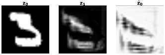
This new ODE-related perspective can lead to new insights regarding stability and trainability of networks, as well as new network architectures inspired by ODE discretization schemes. However, there is a major challenge in implementation of neural ODEs. Computing the gradients of an ODE layer through backpropagation requires storing all intermediate ODE solutions in time (either through auto differentiation or an adjoint method §II-A), which can easily lead to prohibitive memory costs. For example, if we were to use two forward Euler time steps for Eq. 1b, we would have $z_{1/2}=z_{0}+1/2f(z_{0},\theta)$ and $z_{1}=z_{1/2}+1/2f(z_{1/2},\theta)$. We need to store all $z_{0}$, $z_{1/2}$ and $z_{1}$ in order to compute the gradient with respect the model weights $\theta$. Therefore, if we take $N_{t}$ time steps then we require $\mathcal{O}(N_{t})$ storage per ODE block. If we have $L$ residual blocks, each being a separate ODE, the storage requirements can increase from $\mathcal{O}(L)$ to $\mathcal{O}(LN_{t})$.

Figure 2: A residual block of SqueezeNext [15] is shown. The input activation is denoted by $z_{n}$, along with the intermediate values of $z_{n}^{1},\cdots,z_{n}^{5}$. The output activation is denoted by $z_{n+1}=z_{n}^{5}+z_{n}$. In the second row, we show a compact representation, by denoting the convolutional blocks as $f(z)$. This residual block could be thought of solving an ODE Eq. 1b with an Euler scheme.

In the recent work of [8], an adjoint based backpropagation method was proposed to address this challenge; it only requires $\mathcal{O}(L)$ memory to compute the gradient with respect $\theta$, thus significantly outperforming existing backpropagation implementations. The basic idea is that instead of storing $z(t)$, we store only $z(t=1)$ and then we reverse the ODE solver in time by solving $\frac{dz}{dt}=-f(z(t),\theta)$, in order to reconstruct $z(t=0)$ and evaluate the gradient. However, we will show that using this approach does not work for any value $\theta$ for a general NN model. It may lead to significant ($\mathcal{O}(1)$) errors in the gradient because reversing the ODE may not be possible and, even if it is, numerical discretization errors may cause the gradient to diverge.

Here we discuss the underlying issues and then present ANODE, an Adjoint based Neural ODE framework that employs a classic “checkpointing” scheme that addresses the memory problem and results in correct gradient calculation no matter the structure of the underlying network. In particular, we make the following contributions:

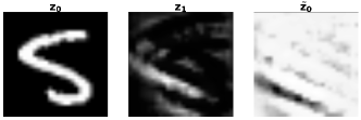
• We show that neural ODEs with ReLU activations may not be reversible (see §III). Attempting to solve such ODEs backwards in time, so as to recover activations $z(t)$ in earlier layers, can lead to mathematically incorrect gradient information. This in turn may lead to divergence of the training. This is illustrated in Figs. 1, 3, 4, and 7.

• We show that even for general convolution/activation operators, the reversibility of neural ODE may be numerically unstable. This is due to possible ill-conditioning of the reverse ODE solver, which can amplify numerical noise over large time horizons (see §III). An example of instability is shown in Fig.  1. Note that this instability cannot be resolved by using adaptive time stepping as shown in Fig.  7.

• We discuss an important consistency problem between discrete gradient and continuous gradient, and show that ignoring this inconsistency can lead to divergent training. We illustrate that this problem stems from well established issue related to the difference between “Optimize-Then-Discretize” differentiation methods versus “Discretize-Then-Optimize” differentiation methods (see §IV).

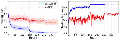
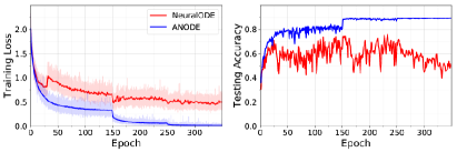
• We present ANODE, which is a neural ODE framework with checkpointing that uses “Discretize-Then-Optimize” differentiation method (see §V). ANODE avoids the above problem, and squeezes the memory footprint to $\mathcal{O}(L)+\mathcal{O}(N_{t})$ from $\mathcal{O}(LN_{t})$, without suffering from the above problems. This footprint can be further reduced with additional computational cost through logarithmic checkpointing methods. Preliminary tests show efficacy of our approach. A comparison between ANODE and neural ODE [8] is shown in Fig.  3, 4.

I-A Related Work

ODEs: In [27], the authors observed that residual networks can be viewed as a forward Euler discretization of an ODE. The stability of the forward ODE problem was discussed in [20, 5], where the authors proposed architectures that are discrete Hamiltonian systems and thus are both stable and reversible in both directions. In an earlier work, a similar reversible architecture was proposed for unsupervised generative models [11, 12]. In [16], a reversible architecture was used to design a residual network to avoid storing intermediate activations.

Adjoint Methods: Adjoint based methods have been widely used to solve problems ranging from classical optimal control problems [22] and large scale inverse problems [2, 3], to climate simulation [6, 21]. Despite their prohibitive memory footprint, adjoint methods were very popular in the nineties, mainly due to the computational efficiency for computing gradients as compared to other methods. However, the limited available memory at the time, prompted researchers to explore alternative approaches to use adjoint without having to store all of the forward problem’s trajectory in time. For certain problems such as climate simulations, this is still a major consideration, even with the larger memory available today. A seminal work that discussed an efficient solution to overcome this memory overhead was first proposed in [17], with a comprehensive analysis in [18]. It was proved that for given a fixed memory budget, one can obtain optimal computational complexity using a binomial checkpointing method.

The checkpointing method was recently re-discovered in machine learning for backpropagation through long recurrent neural networks (NNs) in [24], by checkpointing a square root of the time steps. During backpropagation, the intermediate activations were then computed by an additional forward pass on these checkpoints. Similar approaches to the optimal checkpointing, originally proposed in [17, 18], were recently explored for memory efficient NNs in [9, 19].

II Problem Description

We first start by introducing some notation. Let us denote the input/output training data as $x\in{\mathcal{R}}^{d}_{x}$ and $y\in{\mathcal{R}}^{d}_{y}$, drawn from some unknown probability distribution $P(x,y):{\mathcal{R}}^{d}_{x}\times{\mathcal{R}}^{d}_{y}\rightarrow[0,1]$. The goal is to learn the mapping between $y$ and $x$ via a model $F(\theta)$, with $\theta$ being the unknown parameters. In practice we do not have access to the joint probability of $P(x,y)$, and thus we typically use the empirical loss over a set of $m$ training examples:

$$\min_{\theta}{\mathcal{J}}(\theta,x,y)=\frac{1}{m}\sum_{i=1}^{m}\ell(F(\theta,x_{i}),y_{i})+{\mathcal{R}}(\theta),$$ (2)

where the last term, ${\mathcal{R}}(\theta)$, is some regularization operator such as weight decay. This optimization problem is solved iteratively, starting with some (random) initialization for $\theta$. Using this initialization for the network, we then compute the activation of each layer by solving Eq. 1b forward in time (along with possibly other transition, pooling, or fully connected layers). After the forward solve, we obtain $F(z)$, which is the prediction of the NN (e.g. a vector of probabilities for each class). We can then compute a pre-specified loss (such as cross entropy) between this prediction and the ground truth training data, $y$. To train the network, we need to compute the gradient of the loss with respect to model parameters, $\theta$. This would require backpropogating the gradient through ODE layers.

A popular iterative scheme for finding optimal value for $\theta$ is Stochastic Gradient Descent (SGD), where at each iteration a mini-batch of size $B$ training examples are drawn, and the loss is evaluated over this mini-batch, using a variant of the following update equation:

$$\theta^{\text{new}}=\theta^{\text{old}}-\eta\frac{1}{B}\sum^{B}_{i=1}\nabla_{\theta}\ell(F(\theta,x_{i}),y_{i}).$$ (3)

Typically the gradient is computed using chain rule by constructing a graph of computations during the forward pass. For ODE based models, the forward operator would involve integration of Eq. 1b. To backpropagate through this integration, we need to solve a so called adjoint equation. However, as we will demonstrate, the memory requirement can easily become prohibitive even for shallow NNs.

II-A Adjoint Based Backpropogation

We first demonstrate how backpropogation can be performed for an ODE layer. For clarity let us consider a single ODE in isolation and denote its output activation with $z_{1}$ which is computed by solving Eq. 1b forward in time. During backpropogation phase, we are given the gradient of the loss with respect to output, $\frac{\partial{\mathcal{J}}}{\partial z_{1}}$, and need to compute two gradients: (i) gradient w.r.t. model parameters $\frac{\partial{\mathcal{J}}}{\partial\theta}$ which will be used in Eq. 3 to update $\theta$, and (ii) backpropogate the gradient through the ODE layer and compute $\frac{\partial{\mathcal{J}}}{\partial z_{0}}$. To compute these gradients, we first form the Lagrangian for this problem defined as:

$${\mathcal{L}}={\mathcal{J}}(z_{1},\theta)+\int_{0}^{1}\alpha(t)\cdot\left(\frac{dz}{dt}-f(z,\theta)\right)dt,$$ (4)

where $\alpha$ is the so called “adjoint” variable. Using the Lagrangian removes the ODE constraints and the corresponding first order optimality conditions could be found by taking variations w.r.t. state, adjoint, and NN parameters (the so called Karush-Kuhn-Tucker (KKT) conditions):

$$\left\{\begin{array}[]{@{}lll@{}}\displaystyle{\frac{\partial{\mathcal{L}}}{\partial z}}&=0\quad\Rightarrow\quad\ \textrm{adjoint equations \ }\\ \displaystyle{\frac{\partial{\mathcal{L}}}{\partial\theta}}&=0\quad\Rightarrow\quad\ \textrm{inversion equation}\\ \displaystyle{\frac{\partial{\mathcal{L}}}{\partial\alpha}}&=0\quad\Rightarrow\quad\ \textrm{state equations \ \ \ }\end{array}\right.$$

This results in the following system of ODEs:

$$\frac{\partial z}{\partial t}+f(z,\theta)=0,\quad t\in(0,1]$$ (5a)

$$-\frac{\partial\alpha(t)}{\partial t}-\frac{\partial f}{\partial z}^{T}\alpha=0,\quad t\in[0,1)$$ (5b)

$$\alpha_{1}+\frac{\partial J}{\partial z_{1}}=0,$$ (5c)

$$g_{\theta}=\frac{\partial R}{\partial\theta}-\int_{0}^{1}\frac{\partial f}{\partial\theta}^{T}\alpha$$ (5d)

For detailed derivation of the above equations please see Appendix §A-B. Computation of the gradient follows these steps. We first perform the forward pass by solving Eq. 5a. Then during backpropogation we are given the gradient w.r.t. the output activation, i.e., $\frac{\partial J}{\partial z_{1}}$, which can be used to compute $\alpha_{1}$ from Eq. 5c. Using this terminal value condition, we then need to solve the adjoint ODE Eq. 5b to compute $\alpha_{0}$ which is equivalent to backpropogating gradient w.r.t. input. Finally the gradient w.r.t. model parameters could be computed by plugging in the values for $\alpha(t)$ and $z(t)$ into Eq. 5d.

It can be clearly seen that solving either Eq. 5b, or Eq. 5d requires knowledge of the activation throughout time, $z(t)$. Storage of all activations throughout this trajectory in time leads to a storage complexity that scales as $\mathcal{O}(LN_{t})$, where $L$ is the depth of the network (number of ODE blocks) and $N_{t}$ is the number of time steps (or intermediate discretization values) which was used to solve Eq. 1b. This can quickly become very expensive even for shallow NNs, which has been the main challenge in deployment of neural ODEs.

In the recent work of [8], an idea was presented to reduce this cost down to $\mathcal{O}(L)$ instead of $\mathcal{O}(LN_{t})$. The method is based on the assumption that the activation functions $z(t)$ can be computed by solving the forward ODE backwards (aka reverse) in time. That is given $z(t=1)$, we can solve Eq. 1b backwards, to obtain intermediate values of the activation function. However, as we demonstrate below this method may lead to incorrect/noisy gradient information for general NNs.

III Can we reverse an ODE?

Here we summarize some well-known results for discrete and continuous dynamical systems. Let $\frac{dz(t)}{dt}=f(z(t))$, with $z\in\mathbb{R}^{n}$, be an autonomous ODE where $f(z)$ is locally Lipschitz continuous. The Picard-Linderlöf theorem states that, locally, this ODE has a unique solution which depends continuously on the initial condition [1] (page 214). The flow $\phi(z_{0},s)$ of this ODE is defined as its solution with $z(t=0)=z_{0}$ with time horizon $s$ and is a mapping from $\mathbb{R}^{n}$ to $\mathbb{R}^{n}$ and satisfies $\phi(z_{0},s+t)=\phi(\phi(z_{0},s),t)$.

If $f$ is $C^{1}$ and $z_{0}$ is the initial condition, then there is a time horizon $I_{0}:=[0,\tau]$ ($\tau$, which depends on $z_{0}$) for which $\phi$ is a diffeomorphism, and thus for any $t\in I_{0}$ $\phi(\phi(z_{0},t),-t)=z_{0}$ [1] (page 218). In other words, this result asserts that if $f$ is smooth enough, then, up to certain time horizon, which depends on the initial condition, the ODE is reversible. For example, consider the following ODE with $f\in C^{\infty}$ : $\frac{dz(t)}{dt}=z(t)^{3}$, with $z(0)=z_{0}$. We can verify that the flow of this ODE is given by $\phi(z_{0},t)=\frac{z_{0}}{\sqrt{1-2z_{0}^{2}t}}$, which is only defined for $t<\frac{1}{2z_{0}^{2}}$. This simple example reveals a first possible source of problems since the $\theta$ and time horizon (which defines $f$) will be used for all points $z_{0}$ in the training set and reversibility is not guaranteed for all of them.

It turns that this local reversibility (i.e., the fact that the ODE is reversible only if the time horizon is less or equal to $\tau$) can be extended to Lipschitz functions [4]. (In the Lipschitz case, the flow and its inverse are Lipschitz continuous but not diffeomorphic.) This result is of particular interest since the ReLU activation is Lipschitz continuous. Therefore, an ODE with $f(z)=\max(0,\lambda z)$ (for $\lambda\in\mathbb{R}$) is reversible.

The reverse flow can be computed by solving $\frac{dz}{ds}=-f(z(s))$ with initial condition $z(s=0)=z(\tau)$ (i.e., the solution of the forward ODE at $t=\tau$). Notice the negative sign in the right hand side of the reverse ODE. The reverse ODE is not the same as the forward ODE. The negative sign in the right hand side of the reverse ODE, reverses the sign of the eigenvalues of the derivative of $f$. If the Lipschitz constant is too large, then reversing the time may create numerical instability that will lead to unbounded errors for the reverse ODE, even if the forward ODE is stable and easy to resolve numerically. To illustrate this consider a simple example. The solution of linear ODEs of the form $dz/dt=\lambda z$, is $z(t)=z_{0}\exp(\lambda t)$. If $\lambda<0$, resolving $z(t)$ with a simple solver is easy. But reversing it is numerically unstable (since small errors get amplified exponentially fast). Consider $\lambda=-100$, i.e., $dz/dt=-100z$, with $z(0)=1$ and unit time horizon. A simple way to measure the reversibility of the ODE is the following error metric:

$$\rho(z(0),t)=\frac{\|\phi(\phi(z(0),t),-t)-z(0)\|_{2}}{\|z(0)\|_{2}}.$$ (6)

For $t=1$, Resolving both forward and backward flows up to 1% requires about 200,000 time steps (using either an explicit or an implicit scheme). For $\lambda=-1e4$, the flow is impossible to reverse numerically in double precision. Although these example might seem to be contrived instabilities, they are actually quite common in dynamical systems. For example, the linear heat equation can result in much larger $\lambda$ values and is not reversible [13].

These numerical issues from linear ODEs extend to ReLU ODEs. Computing $\phi(\phi(z_{0},1),-1)$ for $\frac{dz(t)}{dt}=-\max(0,10z(t)),\quad z(0)=1,\quad t\in(0,1],$ with $\mathtt{ode45}$ method leads to 1% error $|\phi(\phi(z(0),1),-1)-z(0)|$ with 11 time steps; and 0.4% error with 18 time steps. Single machine precision requires 211 time steps using MATLAB’s $\mathtt{ode45}$ solver. As a second example, consider

$$\frac{dz(t)}{dt}=\max(0,Wz(t)),$$ (7)

where $z(t)\in\mathbb{R}^{n}$ and $W\in\mathbb{R}^{n\times n}$ is a Gaussian random matrix, which is used sometimes as initialization of weights for both fully connected and convolutional networks. As shown in [26], $\|W\|_{2}$ grows as $\sqrt{n}$ and numerically reversing this ODE is nearly impossible for $n$ as small as 100 (it requires 10,000 time steps to get single precision accuracy in error defined by equation 6). Normalizing $W$ so that $\|W\|_{2}=\mathcal{O}(1)$, makes the reversion numerically possible.

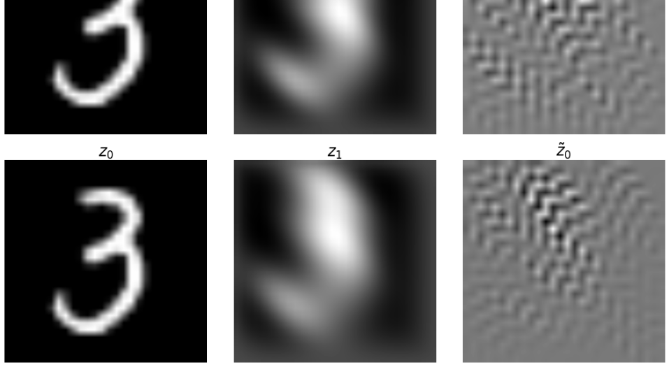
A complementary way to view these problems is by considering the reversibility of discrete dynamical systems. For a repeated map $F^{(n)}=F\circ F\circ F\circ\cdots\circ F$ the reverse map can be defined as $F^{(-n)}=F^{-1}\circ F^{-1}\circ F^{-1}\circ\cdots\circ F^{-1}$, which makes it computationally expensive and possibly unstable if $F$ is nearly singular. For example, consider the map $F(z)=z+a\max(0,z)$ which resembles a single forward Euler time step of a ReLU residual block. Notice that simply reversing the sign is not sufficient to recover the original input. It is easy to verify that if $z_{0}>0$ then $z_{0}\neq z_{1}-a\max(0,z_{1})$ results in error of magnitude $|a^{2}z_{0}|$. If we want to reverse the map, we need to solve $y+a\max(0,y)=x_{1}$ for $y$ given $x_{1}$. Even then this system in general may not have a unique solution (e.g., $-2=y-3\max(0,y)$ is satisfied for both $y=-2$ and $y=1$). Even if it has a unique solution (for example if $F(z)=z+f(z)$ and $f(z)$ is a contraction [1] (page 124)) it requires a nonlinear solve, which again may introduce numerical instabilities. In a practical setting an ODE node may involve several ReLUs, convolutions, and batch normalization, and thus its reversibility is unclear. For example, in NNs some convolution operators resemble differentiation operators, that can lead to very large $\lambda$ values (similar to the heat equation). A relevant example is a $3\times 3$ convolution that is equivalent to the discretization of a Laplace operator. Another example is a non-ReLU activation function such as Leaky ReLU. We illustrate the latter case in Fig.  1 (second row). We consider a residual block with Leaky ReLU using an MNIST image as input. As we can see, solving the forward ODE backwards in time leads to significant errors. In particular note that this instability cannot be resolved through adaptive time stepping. We show this for different activation functions in Fig.  7.

Figure 3: Training loss (left) and Testing accuracy (right) for on Cifar-10. We consider a SqueezeNext network where non-transition blocks are replaced with an ODE block, solved with Euler method (top) and RK-2 (Trapezoidal method). As one can see, the gradient computed using [8] results in sub-optimal performance, compared to ANODE. Furthermore, testing [8] with RK45 lead to divergent training in the first epoch.

Without special formulations/algorithms, ODEs and discrete dynamical systems can be problematic to reverse. Therefore, computing the gradient (see Eq. 5b and Eq. 5d), using reverse flows may lead to $\mathcal{O}(1)$ errors. In [8] it was shown that such approach gives good accuracy on MNIST. However, MNIST is a simple dataset and as we will show, testing a slightly more complex dataset such as Cifar-10 will clearly demonstrates the problem. It should also be noted that it is possible to avoid this stability problem, but it requires either a large number of time steps or specific NN design [11, 16, 5]. In particular, Hamiltonian ODEs and the corresponding discrete systems [20] allow for stable reversibility in both continuous and discrete settings. Hamiltonian ODEs and discrete dynamical systems are reversible to machine precision as long as appropriate time-stepping is used. A shortcoming of Hamiltonian ODEs is that so far their performance has not matched the state of the art in standard benchmarks.

In summary, our main conclusion of this section is that activation functions and ResNet blocks that are Lipschitz continuous could be reversible in theory (under certain constraints for magnitude of the Lipschitz constant), but in practice there are several complications due to instabilities and numerical discretization errors. Next, we discuss another issue with computing derivatives for neural ODEs.

IV Optimize-Then-Discretize versus Discretize-Then-Optimize

An important consideration with adjoint methods is the impact of discretization scheme for solving the ODEs. For a general function, we can neither solve the forward ODE of Eq. 1b nor the adjoint ODE of Eq. 5b analytically. Therefore, we have to solve these ODEs by approximating the derivatives using variants of finite difference schemes such as Euler method. However, a naive use of such methods can lead to subtle inconsistencies which can result in incorrect gradient signal. The problem arises from the fact that we derive the continuous form for the adjoint in terms of an integral equation. This approach is called Optimize-Then-Discretize (OTD). In OTD method, there is no consideration of the discretization scheme, and thus there is no guarantee that the finite difference approximation to the continuous form of the equations would lead to correct gradient information. We show a simple illustration of the problem by considering an explicit Euler scheme with a single time step for solving Eq. 1b:

$$z_{1}=z_{0}+f(z_{0},\theta).$$ (8)

During gradient backpropogation we are given $\frac{\partial L}{\partial z_{1}}$, and need to compute the gradient w.r.t. input (i.e. $z_{0}$). The correct gradient information can be computed through chain rule as follows:

$$\frac{\partial L}{\partial z_{0}}=\frac{\partial L}{\partial z_{1}}(I+\frac{\partial f(z_{0},\theta)}{\partial z_{0}}).$$ (9)

If we instead attempt to compute this gradient with the OTD adjoint method we will have:

$$\alpha_{0}=\alpha_{1}(I+\frac{\partial f(z_{1},\theta)}{\partial z_{1}}),$$ (10)

where $a_{1}=-\frac{\partial L}{\partial z_{1}}$. It can be clearly seen that the results from DTO approach (Eq. 9), and OTD (Eq. 10) can be completely different. This is because in general $\frac{\partial f(z_{1},\theta)}{\partial z_{1}}\neq\frac{\partial f(z_{0},\theta)}{\partial z_{0}}$. In fact using OTD’s gradient is as if we backpropogate the gradient by incorrectly replacing input of the neural network with its output. Except for rare cases [14], the error in OTD and DTO’s gradient scales as $\mathcal{O}(dt)$. Therefore, this error can become quite large for small time step sizes.

This inconsistency can be addressed by deriving discretized optimality conditions, instead of using continuous form. This approach is commonly referred to as Discretize-Then-Optimize (DTO). Another solution is to use self adjoint discretization schemes such as RK2 or Implicit schemes. However, the latter methods can be expensive as they require solving a system of linear equations for each time step of the forward operator. For discretization schemes which are not self adjoint, one needs to solve the adjoint problem derived from DTO approach, instead of the OTD method.

Figure 4: Training loss (left) and Testing accuracy (right) for on Cifar-10. We consider a ResNet-18 network where non-transition blocks are replaced with an ODE block, solved with Euler method. As one can see, the gradient computed using [8] results in sub-optimal performance, compared to ANODE. Furthermore, testing [8] with RK45 leads to divergent training in the first epoch.

Figure 5: Training loss (left) and Testing accuracy (right) for on Cifar-100. We consider a ResNet-18 network where non-transition blocks are replaced with an ODE block, solved with the Euler method. As one can see, the gradient computed using [8] results in sub-optimal performance, compared to ANODE. Furthermore, testing [8] with RK45 leads to divergent training in the first epoch.

Figure 6: Illustration of checkpointing scheme for two ODE blocks with five time steps. Each circle denotes a complete residual block (Fig.  2). Solid circles denote activations for an entire residual block, along with intermediate values based on the discretization scheme, that are stored in memory during forward pass (blue arrows). For backwards pass, denoted by orange arrows, we first recompute the intermediate activations of the second block, and then solve the adjoint equations using $\frac{dL}{dz_{2}}$ as terminal condition and compute $\frac{dL}{dz_{1}}$. Afterwards, the intermediate activations are freed in the memory and the same procedure is repeated for the first ODE block until we compute $\frac{dL}{dz_{0}}$. For cases with scarce memory resources, a logarithmic checkpointing can be used [17, 18].

V ANODE

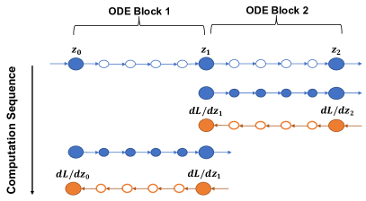
As discussed above, the main challenge with neural ODEs is the prohibitive memory footprint during training, which has limited their deployment for training deep models. For a NN with $L$ ODE layers, the memory requirement is $\mathcal{O}(LN_{t})$, where $N_{t}$ is the total number of time steps used for solving Eq. 1b. We also need to store intermediate values between the layers of a residual block ($z_{n}^{i}$ in Fig.  2), which adds a constant multiplicative factor. Here, we introduce ANODE, a neural ODE with checkpointing that squeezes the memory footprint to $\mathcal{O}(L)+\mathcal{O}(N_{t})$, with the same computational complexity as the method proposed by [8], and utilizes the DTO method to backpropogate gradient information. In ANODE, the input activations of every ODE block are stored in memory, which will be needed for backpropogating the gradient. This amounts to the $\mathcal{O}(L)$ memory cost Fig.  6. The backpropogation is performed in multi-stages. For each ODE block, we first perform a forward solve on the input activation that was stored, and save intermediate results of the forward pass in memory (i.e. trajectory of Eq. 1b along with $z_{n}^{i}$ in Fig.  2). This amounts to $\mathcal{O}(N_{t})$ memory cost. This information is then used to solve the adjoint backwards in time using the DTO method through automatic differentiation. Once we compute the gradients for every ODE block, this memory is released and reused for the next ODE block. Our approach gives the correct values for ReLU activations, does not suffer from possible numerical instability incurred by solving Eq. 1b backwards in time, and gives correct numerical gradient in line with the discretization scheme used to solve Eq. 1b.

For cases where storing $\mathcal{O}(N_{t})$ intermediate activations is prohibitive, we can incorporate the classical checkpointing algorithm algorithms [17, 18]. For the extreme case where we can only checkpoint one time step, we have to recompute $\mathcal{O}(N_{t}^{2})$ forward time stepping for the ODE block. For the general case where we have $1<m<N_{t}$ memory available, a naive approach would be to checkpoint the trajectory using equi-spaced discretization. Afterwards, when the trajectory is needed for a time point that was not checkpointed, we can perform a forward solve using the nearest saved value. However, this naive approach is not optimal in terms of additional re-computations that needs to be done. In the seminal work of [17, 18] an optimal strategy was proposed which carefully chooses checkpoints, such that minimum additional re-computations are needed. This approach can be directly incorporated to neural ODEs for cases with scarce memory resources.

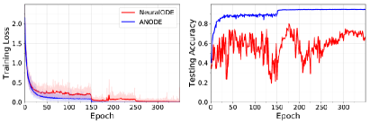
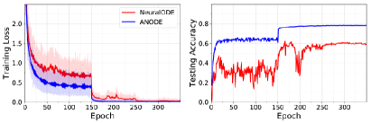
Finally we show results using ANODE, shown in Fig.  3 for a SqueezeNext network on Cifar-10 dataset. Here, every (non-transition) block of SqueezeNext is replaced with an ODE block, and Eq. 1b is solved with Euler discretization, along with an additional experiment where we use RK2 (Trapezoidal rule). As one can see, ANODE results in a stable training algorithm that converges to higher accuracy as compared to the neural ODE method proposed by [8]. Furthermore, Figure 4 shows results using a variant of ResNet-18, where the non-transition blocks are replaced with ODE blocks, on Cifar-10 dataset. Again we see a similar trend, where training neural ODEs results in sub-optimal performance due to the corrupted gradient backpropogation. We also present results on Cifar-100 dataset in Fig.  5 with the same trend. The reason for unconditional stability of ANODE’s gradient computation is that we compute the correct gradient (DTO) to machine precision. However, the neural ODE [7] does not provide any such guarantee, as it changes the calculation of the gradient algorithm which may lead to incorrect descent signal.

VI Conclusions

Neural ODEs have the potential to transform NNs architectures, and impact a wide range of applications. There is also the promise that neural ODEs could result in models that can learn more complex tasks. Even though the link between NNs and ODEs have been known for some time, their prohibitive memory footprint has limited their deployment. Here, we performed a detailed analysis of adjoint based methods, and the subtle issues that may arise with using such methods. In particular, we discussed the recent method proposed by [8], and showed that (i) it may lead to numerical instability for general convolution/activation operators, and (ii) the optimize-then-discretize approach proposed can lead to divergence due to inconsistent gradients. To address these issues, we proposed ANODE, a DTO framework for NNs which circumvents these problems through checkpointing and allows efficient computation of gradients without imposing restrictions on the norm of the weight matrix (which is required for numerical stability as we saw for equation 7). ANODE reduces the memory footprint from $\mathcal{O}(LN_{t})$ to $\mathcal{O}(L)+\mathcal{O}(N_{t})$, and has the same computational cost as the neural ODE proposed by [8]. It is also possible to further reduce the memory footprint at the cost of additional computational overhead using classical checkpointing schemes [17, 18]. We discussed results on Cifar-10/100 dataset using variants of Residual and SqueezeNext networks.

Limitations: A current limitation is the stability of solving Eq. 1b forward in time. ANODE does not guarantee such stability as this needs to be directly enforced either directly in the NN architecture (e.g. by using Hamiltonian systems) or implicitly through regularization. Furthermore, we do not consider NN design itself to propose a new macro architecture. However, ANODE provides the means to efficiently perform Neural Architecture Search for finding an ODE based architecture for a given task. Another important observation, is that we did not observe generalization benefit when using more sophisticated discretization algorithms such as RK2/RK4 as compared to Euler which is the baseline method used in ResNet. We also did not observe benefit in using more time steps as opposed to one time step. We believe this is due to staleness of the NN parameters in time. Our conjecture is that the NN parameters need to dynamically change in time along with the activations. We leave this as part of future work.

Appendix A Appendix

Here, we first present the derivation of the continuous Karush-Kuhn-Tucker (KKT) optimality conditions, and then discuss the corresponding Discretize-Then-Optimize formulation.

A-A Extra Results

Figure 7: Demonstration of numerical instability associated with reversing NNs with adaptive RK45 solver. We consider a single residue block with a single $3\times 3$ convolution layers. Each row corresponds to the following setting for activation after this convolution layer: (1) no activation, (2) with ReLu activation, (3) with Leaky ReLu, and (4) with Softplus activation. The first column shows input image that is fed to the residual block, and the corresponding output activation is shown in the second column. The last column shows the result when solving the forward problem backwards as proposed by [8]. One can clearly see that the third column is completely different than the original image shown in the first column. This is due to the fact that one cannot solve a general ODE backwards in time, due to numerical instabilities.

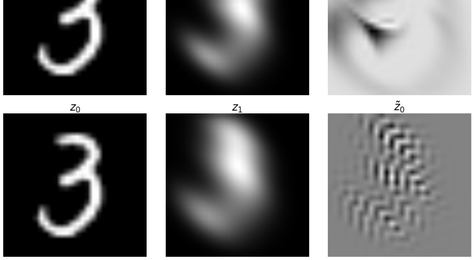
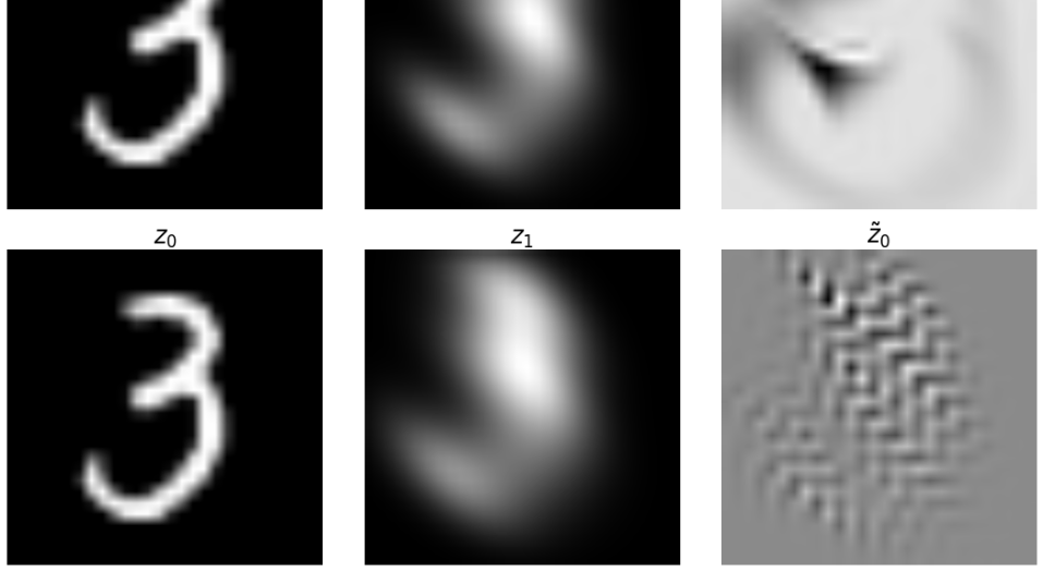
A-B Optimize Then Discretize Approach

In this section, we present a detailed derivation of the optimality conditions corresponding to Eq. 5b. We need to find the so-called KKT conditions, which can be found by finding stationary points of the corresponding Lagrangian, defined as:

$${\mathcal{L}}(z,\alpha,\theta)={\mathcal{J}}(z_{1},\theta)+\int_{0}^{1}\alpha(t)\cdot\left(\frac{dz}{dt}-f(z,\theta)\right)dt.$$ (11)

The optimality conditions correspond to finding the saddle point of the Lagrangian which can be found by taking variations w.r.t. adjoint, state, and NN parameters. Taking variations w.r.t. adjoint is trivial and results in Eq. 5a. By taking variations w.r.t. state variable, z, we will have:

$$\begin{split}\frac{\partial{\mathcal{L}}}{\partial z}\hat{z}=\frac{\partial{\mathcal{J}}}{\partial z_{1}}\hat{z}_{1}+\int_{0}^{1}\alpha(t)\cdot\left(\frac{d\hat{z}}{dt}-f(\hat{z},\theta)\right)dt.\end{split}$$ (12)

Performing integration by parts for $\frac{d\hat{z}}{dt}$ we will obtain:

$$\begin{split}\frac{\partial{\mathcal{L}}}{\partial z}\hat{z}=\frac{\partial{\mathcal{J}}}{\partial z_{1}}\hat{z}_{1}+\int_{0}^{1}\cdot\left(-\frac{d\alpha}{dt}-\frac{\partial f(z,\theta)}{\partial z}^{T}\alpha\right)\hat{z}dt+\alpha_{1}\hat{z}_{1}=0\quad\text{for all}\ \hat{z}\in(0,1].\end{split}$$ (13)

Note that there is no variations for $z_{0}$ as the input is fixed. Now the above equality (aka weak form of optimality) has to hold for all variations of $\hat{z}$ in time. By taking variations for only $\hat{z}_{1}$ and setting $\hat{z}=0$ for $z(t)\in(0,1)$ we will have:

$$\frac{\partial{\mathcal{J}}}{\partial z_{1}}+\alpha_{1}=0.$$ (14)

Note that this is equivalent to Eq. 5c. Furthermore, taking variations by setting $\hat{z}_{1}=0$, we will have:

$$-\frac{d\alpha}{dt}-\frac{\partial f(z,\theta)}{\partial z}^{T}\alpha=0,$$ (15)

which is the same as Eq. 5b. The last optimality condition can be found by imposing stationarity w.r.t. $\theta$:

$$\begin{split}\frac{\partial{\mathcal{L}}}{\partial\theta}\hat{\theta}=\frac{\partial R}{\partial\theta}\hat{\theta}+\int_{0}^{1}\cdot\left(-\frac{\partial f(z,\theta)}{\partial\theta}^{T}\alpha\right)\hat{\theta}dt=0\quad\text{for all}\ \hat{\theta}.\end{split}$$ (16)

Imposing the above for all $\theta$ leads to:

$$g_{\theta}=\frac{\partial R}{\partial\theta}\hat{\theta}-\int_{0}^{1}\frac{\partial f(z,\theta)}{\partial\theta}^{T}\alpha,$$ (17)

which is the same as Eq. 5d. These equation are the so called Optimize-Then-Discretize (OTD) form of the backpropogation. However, using these equations could lead to incorrect gradient, as the choice of discretization creates inconsistencies between continuous form of equations and their corresponding discrete form. This is a known and widely studied issue in scientific computing [14]. The solution to this is to derive the so called Discretize-Then-Optimize (DTO) optimality conditions as opposed to OTD which is discussed next. It must be mentioned that by default, the auto differentiation engines automatically perform DTO. However, deriving the exact equations could provide important insights into the backpropogation for Neural ODEs.

A-C Discretize Then Optimize Approach

Here we show how the correct discrete gradient can be computed via the DTO approach for an Euler time stepping scheme to solve Eq. 1b. Let us assume that the forward pass will take $N_{t}=n+1$ time steps:

$$z_{0}-z_{0}=0$$

$$z_{1}-z_{0}-\Delta tf(z_{0},\theta,t_{0})=0$$

$$\vdots$$

$$z_{n}-z_{n-1}-\Delta tf(z_{n-1},\theta,t_{n-1})=0$$

$$z_{n+1}-z_{n}-\Delta tf(z_{n},\theta,t_{n})=0$$

where $z_{i}$s are the intermediate solutions to Eq. 1b at time points $t=i\Delta t$, and $n$ denotes the $n^{\text{th}}$ time step. Here the dashed line indicate each time step in the forward solve. The corresponding Lagrangian is:

$$\mathcal{L}(z,\theta,\alpha)=\mathcal{J}(z_{n+1})$$

$$+\int_{\Omega}\alpha_{0}(z_{0}-z_{0})d\Omega$$

$$+\int_{\Omega}\alpha_{1}(z_{1}-z_{0}-\Delta tf(z_{0},\theta,t_{0}))d\Omega$$

$$\vdots$$

$$+\int_{\Omega}\alpha_{n}(z_{n}-z_{n-1}-\Delta tf(z_{n-1},\theta,t_{n-1}))d\Omega$$

$$+\int_{\Omega}\alpha_{n+1}(z_{n+1}-z_{n}-\Delta tf(z_{n},\theta,t_{n}))d\Omega,$$

where $d\Omega$ is the spatial domain (for instance the resolution and channels of the activation map in a neural network), $\alpha_{i}$ is the adjoint variable at time points $t=i\Delta t$, and ${\mathcal{J}}$ is the loss which depends directly on the output activation map, $z_{n+1}$.

Now the adjoint equations (first order optimality equation) can be obtained by taking variations w.r.t. adjoint, state and inversion parameters:

$$\left\{\begin{array}[]{@{}lll@{}}\displaystyle{\frac{\partial{\mathcal{L}}}{\partial z_{i}}}&=0\quad\Rightarrow\quad\ \textrm{adjoint equations \ }\\ \displaystyle{\frac{\partial{\mathcal{L}}}{\partial\theta}}&=0\quad\Rightarrow\quad\ \textrm{inversion equation}\\ \displaystyle{\frac{\partial{\mathcal{L}}}{\partial\alpha_{i}}}&=0\quad\Rightarrow\quad\ \textrm{state equations \ \ \ }\end{array}\right.$$

Performing this variations leads to the following ODEs for the adjoint variable:

$$\alpha_{n+1}-\frac{\partial{\mathcal{L}}}{\partial z_{n+1}}=0$$ (19)

$$\alpha_{n}-\alpha_{n+1}(I+\Delta t\frac{\partial f(z_{n},\theta,t_{n})}{\partial z_{n}})=0$$ (20)

$$\vdots$$ (21)

$$\alpha_{1}-\alpha_{2}(I+\Delta t\frac{\partial f(z_{1},\theta,t_{1})}{\partial z_{1}})=0$$ (22)

$$\alpha_{0}-\alpha_{1}(I+\Delta t\frac{\partial f(z_{0},\theta,t_{0})}{\partial z_{0}})=0$$ (23)

To get the DTO gradient, we first need to solve Eq. LABEL:e:forward_dto for every ODE block and store intermediate activation maps of $z_{i}$ for $i=0,\cdots,n+1$. Afterwards we solve Eq. LABEL:e:adjoint_dto starting from the last time step value of $n+1$ and marching backwards in time to compute $\alpha_{0}$, which is basically the gradient w.r.t. the input activation map of $z_{0}$.

References

- [1] Ralph Abraham, Jerrold E Marsden and Tudor Ratiu “Manifolds, tensor analysis, and applications” Springer Science & Business Media, 2007
- [2] George Biros and Omar Ghattas “Parallel Lagrange–Newton–Krylov–Schur Methods for PDE-Constrained Optimization. Part I: The Krylov–Schur Solver” In SIAM Journal on Scientific Computing 27.2 SIAM, 2005, pp. 687–713
- [3] George Biros and Omar Ghattas “Parallel Lagrange–Newton–Krylov–Schur methods for PDE-constrained optimization. Part II: The Lagrange–Newton solver and its application to optimal control of steady viscous flows” In SIAM Journal on Scientific Computing 27.2 SIAM, 2005, pp. 714–739
- [4] Craig Calcaterra and Axel Boldt In Journal of Mathematical Analysis and Applications 338.2, 2008, pp. 1108 –1115
- [5] Bo Chang, Lili Meng, Eldad Haber, Lars Ruthotto, David Begert and Elliot Holtham “Reversible architectures for arbitrarily deep residual neural networks” In Thirty-Second AAAI Conference on Artificial Intelligence, 2018
- [6] Isabelle Charpentier and Mohammed Ghemires “Efficient adjoint derivatives: application to the meteorological model Meso-NH” In Optimization Methods and Software 13.1 Taylor & Francis, 2000, pp. 35–63
- [7] Patrick H Chen and Cho-jui Hsieh “A comparison of second-order methods for deep convolutional neural networks” In openreview under ICLR 2018, 2018
- [8] Tian Qi Chen, Yulia Rubanova, Jesse Bettencourt and David Duvenaud “Neural Ordinary Differential Equations” In arXiv preprint arXiv:1806.07366, 2018
- [9] Tianqi Chen, Bing Xu, Chiyuan Zhang and Carlos Guestrin “Training deep nets with sublinear memory cost” In arXiv preprint arXiv:1604.06174, 2016
- [10] Marco Ciccone, Marco Gallieri, Jonathan Masci, Christian Osendorfer and Faustino Gomez “NAIS-Net: Stable Deep Networks from Non-Autonomous Differential Equations” In arXiv preprint arXiv:1804.07209, 2018
- [11] Laurent Dinh, David Krueger and Yoshua Bengio “NICE: Non-linear independent components estimation” In arXiv preprint arXiv:1410.8516, 2014
- [12] Laurent Dinh, Jascha Sohl-Dickstein and Samy Bengio “Density estimation using Real NVP” In arXiv preprint arXiv:1605.08803, 2016
- [13] Chu-Li Fu, Xiang-Tuan Xiong and Zhi Qian “Fourier regularization for a backward heat equation” In Journal of Mathematical Analysis and Applications 331.1 Elsevier, 2007, pp. 472–480
- [14] A. Gholami “Fast Algorithms for Biophysically-Constrained Inverse Problems in Medical imaging”, 2017
- [15] Amir Gholami, Kiseok Kwon, Bichen Wu, Zizheng Tai, Xiangyu Yue, Peter Jin, Sicheng Zhao and Kurt Keutzer “SqueezeNext: Hardware-Aware Neural Network Design” In arXiv preprint arXiv:1803.10615, 2018
- [16] Aidan N Gomez, Mengye Ren, Raquel Urtasun and Roger B Grosse “The reversible residual network: Backpropagation without storing activations” In Advances in Neural Information Processing Systems, 2017, pp. 2214–2224
- [17] Andreas Griewank “Achieving logarithmic growth of temporal and spatial complexity in reverse automatic differentiation” In Optimization Methods and software 1.1 Taylor & Francis, 1992, pp. 35–54
- [18] Andreas Griewank and Andrea Walther “Algorithm 799: revolve: an implementation of checkpointing for the reverse or adjoint mode of computational differentiation” In ACM Transactions on Mathematical Software (TOMS) 26.1 ACM, 2000, pp. 19–45
- [19] Audrunas Gruslys, Rémi Munos, Ivo Danihelka, Marc Lanctot and Alex Graves “Memory-efficient backpropagation through time” In Advances in Neural Information Processing Systems, 2016, pp. 4125–4133
- [20] Eldad Haber and Lars Ruthotto “Stable architectures for deep neural networks” In Inverse Problems 34.1 IOP Publishing, 2017, pp. 014004
- [21] Jean Philippe Lafore, Joël Stein, Nicole Asencio, Philippe Bougeault, Véronique Ducrocq, Jacqueline Duron, Claude Fischer, Philippe Héreil, Patrick Mascart and Valéry Masson “The Meso-NH atmospheric simulation system. Part I: Adiabatic formulation and control simulations” In Annales Geophysicae 16.1, 1997, pp. 90–109 Springer
- [22] Jacques Louis Lions “Optimal control of systems governed by partial differential equations (Grundlehren der Mathematischen Wissenschaften)” Springer Berlin, 1971
- [23] Yiping Lu, Aoxiao Zhong, Quanzheng Li and Bin Dong “Beyond finite layer neural networks: Bridging deep architectures and numerical differential equations” In arXiv preprint arXiv:1710.10121, 2017
- [24] James Martens and Ilya Sutskever “Training deep and recurrent networks with hessian-free optimization” In Neural networks: Tricks of the trade Springer, 2012, pp. 479–535
- [25] Lars Ruthotto and Eldad Haber “Deep Neural Networks motivated by Partial Differential Equations” In arXiv preprint arXiv:1804.04272, 2018
- [26] Jianhong Shen “On the singular values of Gaussian random matrices” In Linear Algebra and its Applications 326.1-3 Elsevier, 2001, pp. 1–14
- [27] E Weinan “A proposal on machine learning via dynamical systems” In Communications in Mathematics and Statistics 5.1 Springer, 2017, pp. 1–11