Non-Rigid Structure from Motion: Prior-Free Factorization Method Revisited

Suryansh Kumar
Computer Vision Lab, ETH Zürich, Switzerland
sukumar@vision.ee.ethz.ch
Abstract

A simple prior free factorization algorithm [9] is quite often cited work in the field of Non-Rigid Structure from Motion (NRSfM). The benefit of this work lies in its simplicity of implementation, strong theoretical justification to the motion and structure estimation, and its invincible originality. Despite this, the prevailing view is, that it performs exceedingly inferior to other methods on several benchmark datasets [14, 1]. However, our subtle investigation provides some empirical statistics which made us think against such views. The statistical results we obtained supersedes Dai et al.[9] originally reported results on the benchmark datasets by a significant margin under some elementary changes in their core algorithmic idea [9]. Now, these results not only exposes some unrevealed areas for research in NRSfM but also give rise to new mathematical challenges for NRSfM researchers. We argue that by properly utilizing the well-established assumptions about a non-rigidly deforming shape i.e, it deforms smoothly over frames [27] and it spans a low-rank space, the simple prior-free idea can provide results which is comparable to the best available algorithms. In this paper, we explore some of the hidden intricacies missed by Dai et. al. work [9] and how some elementary measures and modifications can enhance its performance, as high as approx. 18% on the benchmark dataset. The improved performance is justified and empirically verified by extensive experiments on several datasets. We believe our work has both practical and theoretical importance for the development of better NRSfM algorithms.

1 Introduction

Notation: The notation used in this paper is similar to Dai et al. work [9] unless otherwise stated.
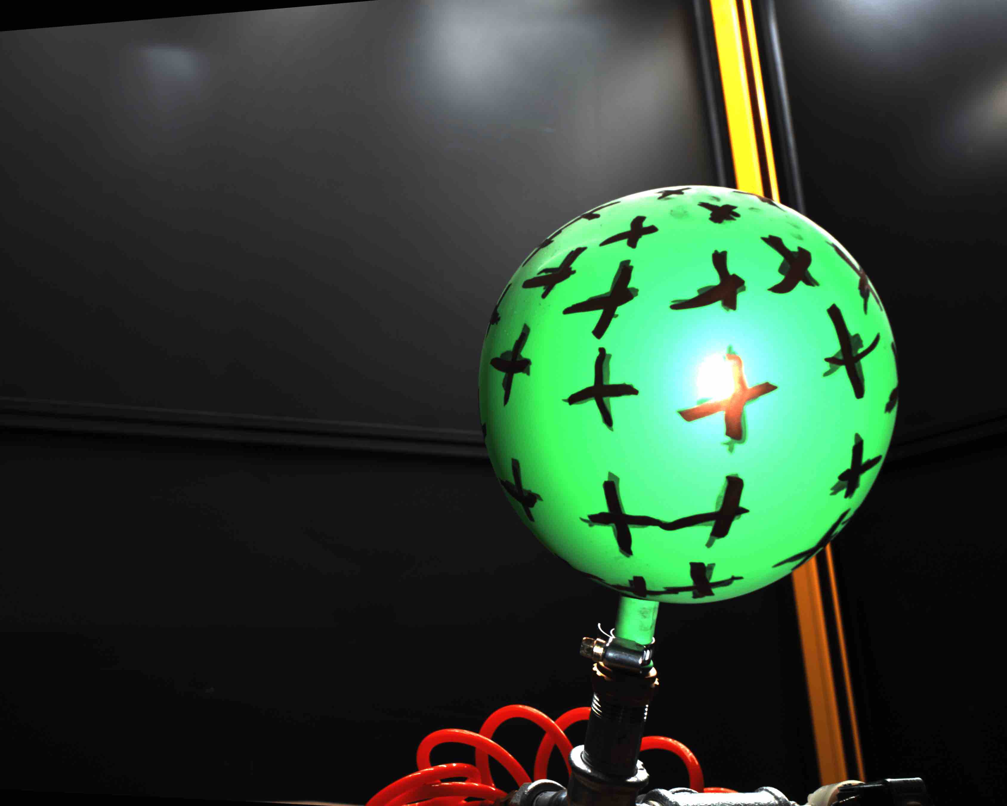
Refer to caption
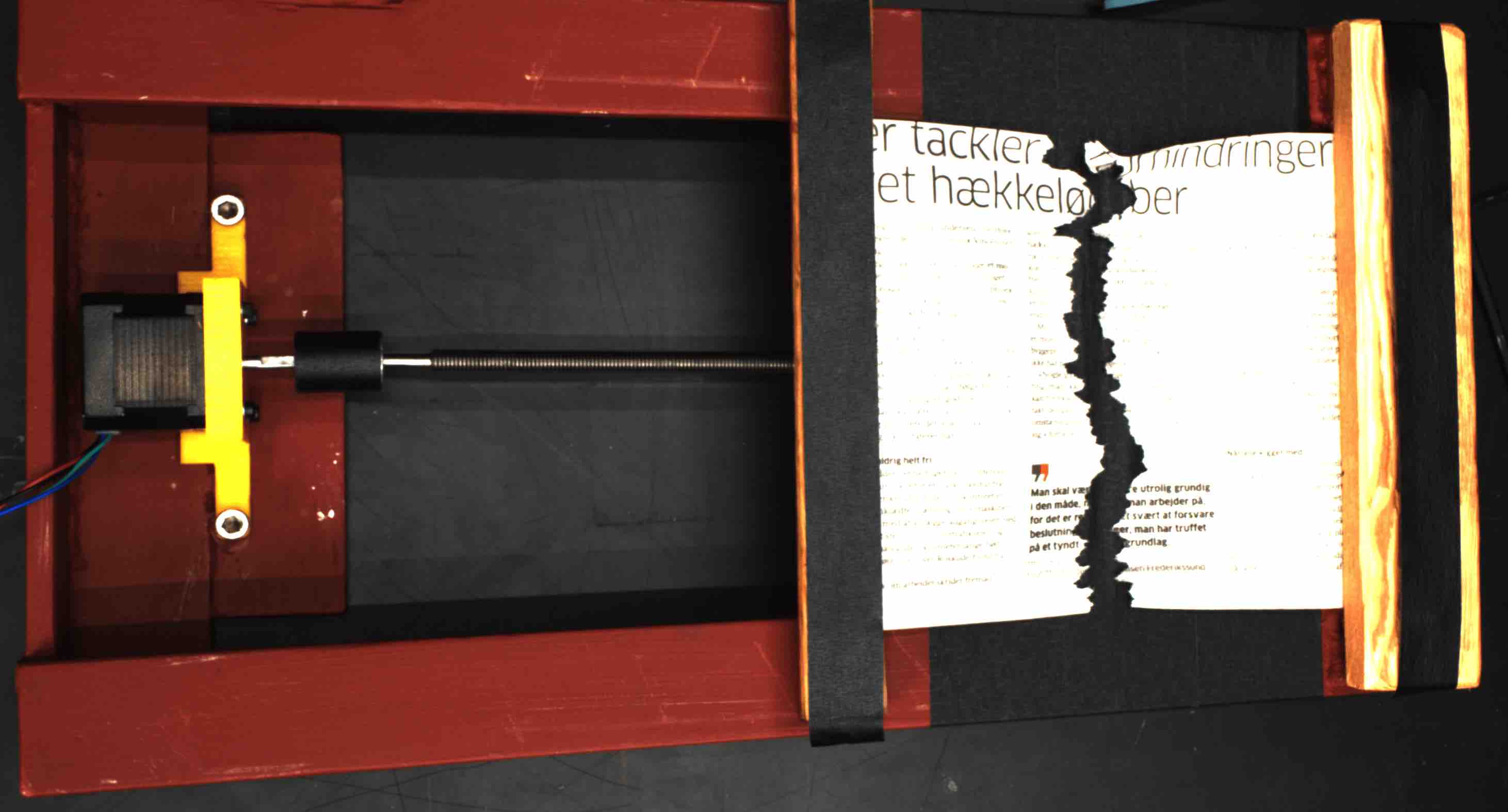
(a) Paper Sequence
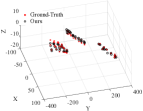
Refer to caption
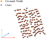
(b) 3D Reconstruction
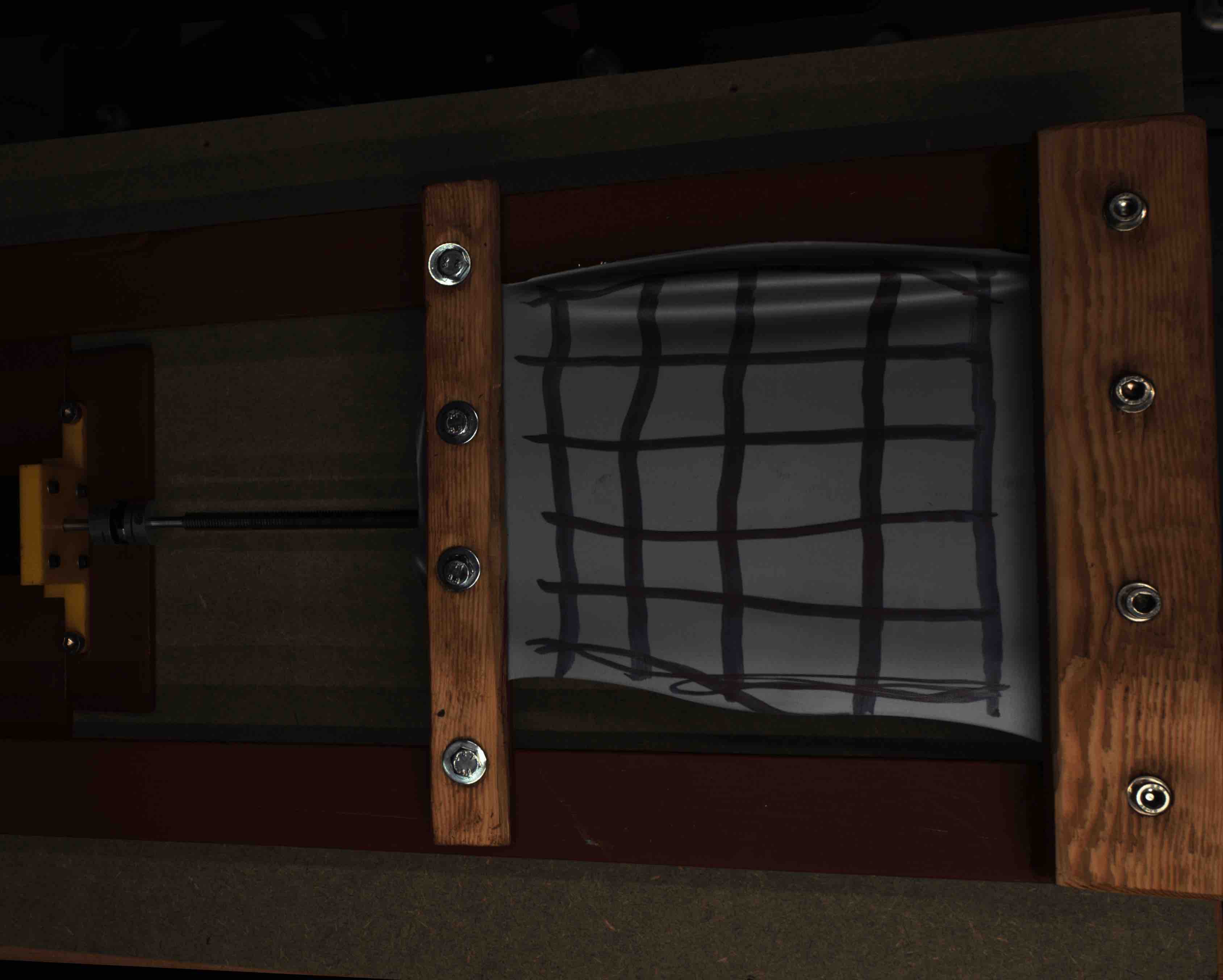
Refer to caption
(c) Tearing Sequence
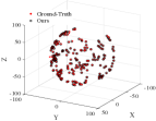
Refer to caption
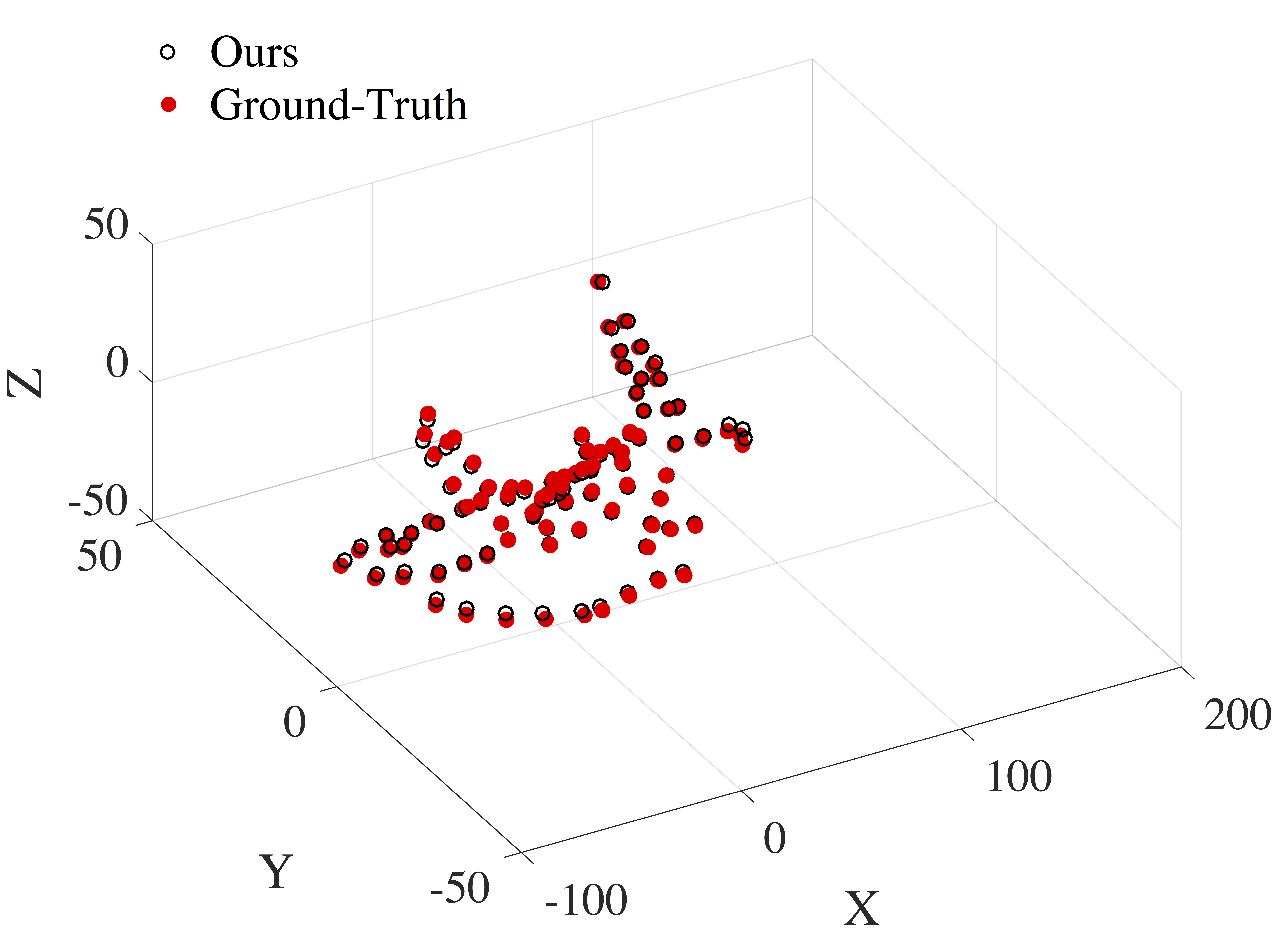
(d) 3D Reconstruction
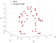
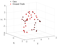
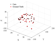
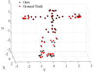
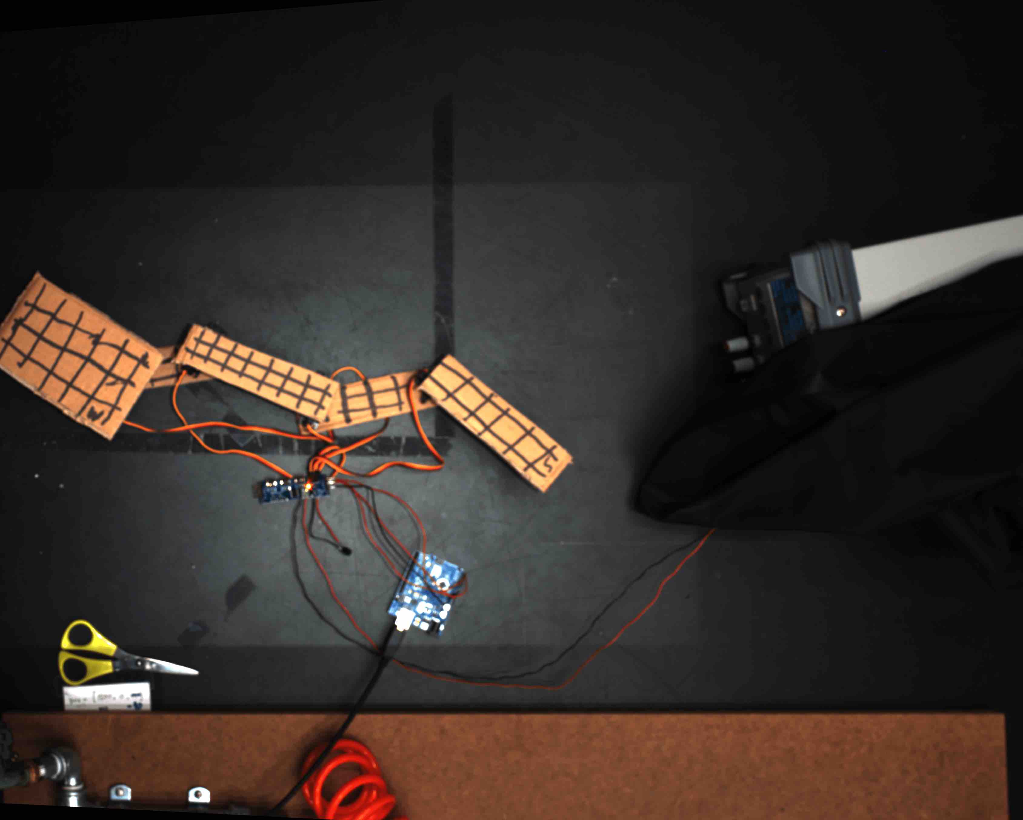
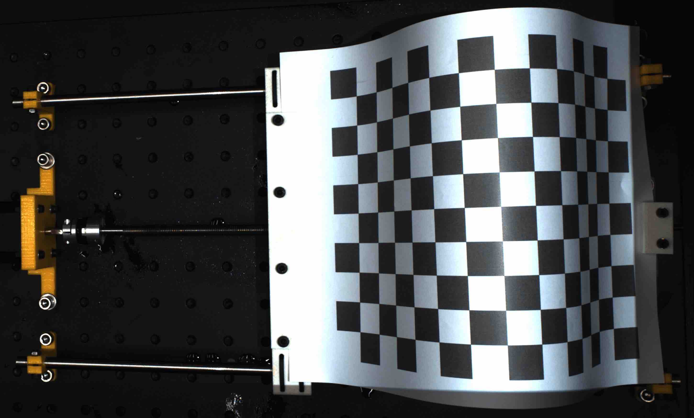
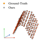
Figure 1: The method recovers 3D dimensional structure of the deforming object over multiple frames. Our elementary but powerful changes provides a substantial improvement in the reconstruction accuracy than the previous results reported for “prior-free" approach. The example images are taken from the recently released NRSfM Challenge Dataset [14]. Our reconstruction results are nearly as good as the best performing algorithm without using very complex and involved mathematical optimization [19].

Non-rigid Structure from Motion (NRSfM) is a well-known problem in geometric computer vision [5, 1, 9, 20, 18]. The goal of this problem is to reconstruct 3D structure of a deforming object using multiple frames. One of the most popular way to solve NRSfM is the matrix factorization approach. The matrix factorization approach to solve this problem dates back to 2000 [5] with no satisfactory solution in place until 2012. In the year 2012, Dai et al. [8] proposed a ground-breaking approach to solve NRSfM. This method for solving NRSfM is now considered as a classical work in NRSfM [9]. In that paper, the camera motion is estimated by imposing the null space constraint and the rank-3 positive semi-definite matrix cone constraint on the Gram matrix (𝚀𝚔subscript𝚀𝚔\mathchoice{\mbox{\bf$\displaystyle\tt Q$}}{\mbox{\bf$\textstyle\tt Q$}}{\mbox{\bf$\scriptstyle\tt Q$}}{\mbox{\bf$\scriptscriptstyle\tt Q$}}_{\mathchoice{\mbox{\bf$\displaystyle\tt k$}}{\mbox{\bf$\textstyle\tt k$}}{\mbox{\bf$\scriptstyle\tt k$}}{\mbox{\bf$\scriptscriptstyle\tt k$}}}). Further, nuclear norm minimization of the reshuffled shape matrix (𝚂superscript𝚂\mathchoice{\mbox{\bf$\displaystyle\tt S$}}{\mbox{\bf$\textstyle\tt S$}}{\mbox{\bf$\scriptstyle\tt S$}}{\mbox{\bf$\scriptscriptstyle\tt S$}}^{\sharp}) was introduced to proffer stronger rank bound on the shape matrix for non-rigid shape estimation. The striking part of their work is that it not only challenged the myth of the inherent basis ambiguity in NRSfM [33] but also supplied a practical “prior-free" algorithm to solve NRSfM. Nonetheless, over years, it was observed that their remarkable theory performs poorly on benchmark datasets [22, 14]. In this paper, our goal is to make “prior-free idea” work well on real world scenarios.

Theoretically, the elementary idea of Dai et al. [9] conveniently encapsulates all the basic intuitions which are required to solve a general NRSfM problem. One may immediately argue on its performance when the deforming shape is composed of a union of low-rank subspace[19, 17, 36, 16, 15]. However, in this paper, we restrict our discussion to the classical representation of a NRSfM problem [5], without paying much attention to, how clustering benefits 3D reconstruction of the non-rigid object and other such notions of compact data representation. The reason for this choice is that the improvement in the performance of a classical baseline shall benefit the methods built on top of it.

The main purpose of this work is to uncover some of the unexplored mathematical intricacies in the prior free factorization approach to NRSfM, and improve on the idea supplied by Dai et al. [9]. Our exposition leads to the possible reasons for its inferior performance on the benchmark datasets [1, 14, 31]. It is shown in this paper that the rotation estimate using Dai et al. work [9] is not unique under the same model complexity prior (𝙺𝙺\textstyle\tt K/rank), and they overlooked to utilize full correction matrix space [4]. Our investigation unveil the possibility of procuring motion that satisfies the well-known assumption of smooth non-rigid deformation of the object [27]. A simple search for the proper column-triplet (triads [4]) for the correction matrix (𝙶𝚔subscript𝙶𝚔\mathchoice{\mbox{\bf$\displaystyle\tt G$}}{\mbox{\bf$\textstyle\tt G$}}{\mbox{\bf$\scriptstyle\tt G$}}{\mbox{\bf$\scriptscriptstyle\tt G$}}_{\mathchoice{\mbox{\bf$\displaystyle\tt k$}}{\mbox{\bf$\textstyle\tt k$}}{\mbox{\bf$\scriptstyle\tt k$}}{\mbox{\bf$\scriptscriptstyle\tt k$}}}) based on the smoothness of camera motion can indeed help improve the accuracy of the algorithm. Further, we argue that the weighted nuclear norm minimization of the shape matrix (𝚂superscript𝚂\mathchoice{\mbox{\bf$\displaystyle\tt S$}}{\mbox{\bf$\textstyle\tt S$}}{\mbox{\bf$\scriptstyle\tt S$}}{\mbox{\bf$\scriptscriptstyle\tt S$}}^{\sharp}) is a far better choice than its global trace norm minimization. Lastly, due to our extensive analysis, we are able to posit some unsolved issues in NRSfM under “prior-free” idea which needs attention for further progress in this field.

In this paper, it is not claimed that we achieve state-of-the-art results on the benchmark datasets using our new approach. However, we empirically show that we can get very close to the best performing approaches and the difference is not very great, without the employment of complex and involved mathematical optimization [19, 22]. In this paper, we also argue that the inferior performance of “prior-free" method may not be due the proposed theoretical idea but because they overlooked some of the mathematical construction in their own formulation, and missed on properly utilizing the well-known assumptions about non-rigidly moving object i.e., smooth deformation [27] and low-rank shape [9]. Hence, the conclusion, understanding, and use of simple “prior-free” algorithm to NRSfM is not complete and precise. Through this work, we try to amend and nullify the prevailing perception about the “prior-free" approach, and how it can be used to its maximum potential. We feel that our paper touches some critical points which are essential to establish a theoretical closure to some of the elementary problems within the factorization approach to NRSfM.

Contribution: Firstly, our work postulates some rectification to the usage of “Intersection Method" [9] to compute camera motion. With the suitable example, we establish that the generalization made on the rotation matrix estimation by Dai et al. work [9] is not convincing and therefore, the knowledge about the strength of “Intersection theorem” is not completely exploited. Secondly, we provide an analytic solution to estimate suitable rotation using Intersection theorem and conjecture some challenges associated with it. Lastly, we propose a weighted nuclear norm minimization problem to estimate non-rigid 3D shape. Our approach shows a substantial improvement in the 3D reconstruction accuracy (nearly 18%). Moreover, we observed performance improvement in the case of noisy and missing trajectories §4.2 (under minor adjustment) using our method.

In this work, our attempt is to make the baseline method111By baseline, we mean the methods that solve NRSfM using its classical representation 𝚆=𝚁𝚂𝚆𝚁𝚂\mathchoice{\mbox{\bf$\displaystyle\tt W$}}{\mbox{\bf$\textstyle\tt W$}}{\mbox{\bf$\scriptstyle\tt W$}}{\mbox{\bf$\scriptscriptstyle\tt W$}}=\mathchoice{\mbox{\bf$\displaystyle\tt R$}}{\mbox{\bf$\textstyle\tt R$}}{\mbox{\bf$\scriptstyle\tt R$}}{\mbox{\bf$\scriptscriptstyle\tt R$}}\mathchoice{\mbox{\bf$\displaystyle\tt S$}}{\mbox{\bf$\textstyle\tt S$}}{\mbox{\bf$\scriptstyle\tt S$}}{\mbox{\bf$\scriptscriptstyle\tt S$}} that have withstood the test of time [30, 5]. more accurate, both in terms of understanding and performance, subject to the mathematical simplicity. To achieve this, we attempt to avoid the usage of complex mathematical notions such as union of independent subspace, dependent subspace representation [36, 19, 21], procrustean normal distribution [22], kernelization [10] etc. Hence, it is simple to understand the theoretical and practical justification of our method. We show that by applying simple but powerful logical and mathematical modifications to the prior free idea [9], we can get close to or even perform better at times than the best available algorithms on the benchmark datasets.

2 Representation and Motion Estimation

1. Classical Representation:

Tomasi and Kanade factorization method to structure-from-motion under orthographic camera projection appropriately summarizes the behavior of the 3D points over frames [30]. The relation between 3D shape, motion and its projection over frames was defined as

𝚆=𝚁𝚂𝚆𝚁𝚂\mathchoice{\mbox{\bf$\displaystyle\tt W$}}{\mbox{\bf$\textstyle\tt W$}}{\mbox{\bf$\scriptstyle\tt W$}}{\mbox{\bf$\scriptscriptstyle\tt W$}}=\mathchoice{\mbox{\bf$\displaystyle\tt R$}}{\mbox{\bf$\textstyle\tt R$}}{\mbox{\bf$\scriptstyle\tt R$}}{\mbox{\bf$\scriptscriptstyle\tt R$}}\mathchoice{\mbox{\bf$\displaystyle\tt S$}}{\mbox{\bf$\textstyle\tt S$}}{\mbox{\bf$\scriptstyle\tt S$}}{\mbox{\bf$\scriptscriptstyle\tt S$}} (1)

where, 𝚆2𝙵×𝙿𝚆superscript2𝙵𝙿\mathchoice{\mbox{\bf$\displaystyle\tt W$}}{\mbox{\bf$\textstyle\tt W$}}{\mbox{\bf$\scriptstyle\tt W$}}{\mbox{\bf$\scriptscriptstyle\tt W$}}\in\mathbb{R}^{2\mathchoice{\mbox{\bf$\displaystyle\tt F$}}{\mbox{\bf$\textstyle\tt F$}}{\mbox{\bf$\scriptstyle\tt F$}}{\mbox{\bf$\scriptscriptstyle\tt F$}}\times\mathchoice{\mbox{\bf$\displaystyle\tt P$}}{\mbox{\bf$\textstyle\tt P$}}{\mbox{\bf$\scriptstyle\tt P$}}{\mbox{\bf$\scriptscriptstyle\tt P$}}} is the measurement matrix formed by stacking all the image coordinates (𝐱=[𝚞,𝚟]𝚃𝐱superscript𝚞𝚟𝚃\mathbf{x}=[\mathchoice{\mbox{\bf$\displaystyle\tt u$}}{\mbox{\bf$\textstyle\tt u$}}{\mbox{\bf$\scriptstyle\tt u$}}{\mbox{\bf$\scriptscriptstyle\tt u$}},\mathchoice{\mbox{\bf$\displaystyle\tt v$}}{\mbox{\bf$\textstyle\tt v$}}{\mbox{\bf$\scriptstyle\tt v$}}{\mbox{\bf$\scriptscriptstyle\tt v$}}]^{\mathchoice{\mbox{\bf$\displaystyle\tt T$}}{\mbox{\bf$\textstyle\tt T$}}{\mbox{\bf$\scriptstyle\tt T$}}{\mbox{\bf$\scriptscriptstyle\tt T$}}}) for ‘𝙿𝙿\textstyle\tt P’ points along ‘𝙵𝙵\textstyle\tt F’ rows i.e., total number of frames. 𝚁=blockdiagonal(𝚁1,𝚁2,..,𝚁𝙵)2𝙵×3𝙵\mathchoice{\mbox{\bf$\displaystyle\tt R$}}{\mbox{\bf$\textstyle\tt R$}}{\mbox{\bf$\scriptstyle\tt R$}}{\mbox{\bf$\scriptscriptstyle\tt R$}}=\textrm{{blockdiagonal}}(\mathchoice{\mbox{\bf$\displaystyle\tt R$}}{\mbox{\bf$\textstyle\tt R$}}{\mbox{\bf$\scriptstyle\tt R$}}{\mbox{\bf$\scriptscriptstyle\tt R$}}_{1},\mathchoice{\mbox{\bf$\displaystyle\tt R$}}{\mbox{\bf$\textstyle\tt R$}}{\mbox{\bf$\scriptstyle\tt R$}}{\mbox{\bf$\scriptscriptstyle\tt R$}}_{2},..,\mathchoice{\mbox{\bf$\displaystyle\tt R$}}{\mbox{\bf$\textstyle\tt R$}}{\mbox{\bf$\scriptstyle\tt R$}}{\mbox{\bf$\scriptscriptstyle\tt R$}}_{\mathchoice{\mbox{\bf$\displaystyle\tt F$}}{\mbox{\bf$\textstyle\tt F$}}{\mbox{\bf$\scriptstyle\tt F$}}{\mbox{\bf$\scriptscriptstyle\tt F$}}})\in\mathbb{R}^{2\mathchoice{\mbox{\bf$\displaystyle\tt F$}}{\mbox{\bf$\textstyle\tt F$}}{\mbox{\bf$\scriptstyle\tt F$}}{\mbox{\bf$\scriptscriptstyle\tt F$}}\times 3\mathchoice{\mbox{\bf$\displaystyle\tt F$}}{\mbox{\bf$\textstyle\tt F$}}{\mbox{\bf$\scriptstyle\tt F$}}{\mbox{\bf$\scriptscriptstyle\tt F$}}} denotes the orthographic camera rotation matrix with each 𝚁𝚒2×3subscript𝚁𝚒superscript23\mathchoice{\mbox{\bf$\displaystyle\tt R$}}{\mbox{\bf$\textstyle\tt R$}}{\mbox{\bf$\scriptstyle\tt R$}}{\mbox{\bf$\scriptscriptstyle\tt R$}}_{\mathchoice{\mbox{\bf$\displaystyle\tt i$}}{\mbox{\bf$\textstyle\tt i$}}{\mbox{\bf$\scriptstyle\tt i$}}{\mbox{\bf$\scriptscriptstyle\tt i$}}}\in\mathbb{R}^{2\times 3} as per frame rotation. 𝚂3𝙵×𝙿𝚂superscript3𝙵𝙿\mathchoice{\mbox{\bf$\displaystyle\tt S$}}{\mbox{\bf$\textstyle\tt S$}}{\mbox{\bf$\scriptstyle\tt S$}}{\mbox{\bf$\scriptscriptstyle\tt S$}}\in\mathbb{R}^{3\mathchoice{\mbox{\bf$\displaystyle\tt F$}}{\mbox{\bf$\textstyle\tt F$}}{\mbox{\bf$\scriptstyle\tt F$}}{\mbox{\bf$\scriptscriptstyle\tt F$}}\times\mathchoice{\mbox{\bf$\displaystyle\tt P$}}{\mbox{\bf$\textstyle\tt P$}}{\mbox{\bf$\scriptstyle\tt P$}}{\mbox{\bf$\scriptscriptstyle\tt P$}}} represent the shape matrix with each row triplet as a 3D shape. This representation was later extended by Bregler et al. [5] to recover non-rigid 3D shapes. More concretely,

𝚆=[𝐱11𝐱1𝙿𝐱𝙵1𝐱𝙵𝙿]=[𝚁1𝚂1..𝚁𝙵𝚂𝙵]=[𝐜11𝚁1𝐜1𝙺𝚁1𝐜𝙵1𝚁𝙵𝐜𝙵𝙺𝚁𝙵][𝙱1..𝙱𝙺]𝚆matrixsubscript𝐱11subscript𝐱1𝙿subscript𝐱𝙵1subscript𝐱𝙵𝙿matrixsubscript𝚁1subscript𝚂1absentsubscript𝚁𝙵subscript𝚂𝙵matrixsubscript𝐜11subscript𝚁1subscript𝐜1𝙺subscript𝚁1subscript𝐜𝙵1subscript𝚁𝙵subscript𝐜𝙵𝙺subscript𝚁𝙵matrixsubscript𝙱1absentsubscript𝙱𝙺\displaystyle\mathchoice{\mbox{\bf$\displaystyle\tt W$}}{\mbox{\bf$\textstyle\tt W$}}{\mbox{\bf$\scriptstyle\tt W$}}{\mbox{\bf$\scriptscriptstyle\tt W$}}=\begin{bmatrix}\mathbf{x}_{11}\dots\mathbf{x}_{1\mathchoice{\mbox{\bf$\displaystyle\tt P$}}{\mbox{\bf$\textstyle\tt P$}}{\mbox{\bf$\scriptstyle\tt P$}}{\mbox{\bf$\scriptscriptstyle\tt P$}}}\\ \dots\\ \mathbf{x}_{\mathchoice{\mbox{\bf$\displaystyle\tt F$}}{\mbox{\bf$\textstyle\tt F$}}{\mbox{\bf$\scriptstyle\tt F$}}{\mbox{\bf$\scriptscriptstyle\tt F$}}1}\dots\mathbf{x}_{\mathchoice{\mbox{\bf$\displaystyle\tt F$}}{\mbox{\bf$\textstyle\tt F$}}{\mbox{\bf$\scriptstyle\tt F$}}{\mbox{\bf$\scriptscriptstyle\tt F$}}\mathchoice{\mbox{\bf$\displaystyle\tt P$}}{\mbox{\bf$\textstyle\tt P$}}{\mbox{\bf$\scriptstyle\tt P$}}{\mbox{\bf$\scriptscriptstyle\tt P$}}}\end{bmatrix}=\begin{bmatrix}\mathchoice{\mbox{\bf$\displaystyle\tt R$}}{\mbox{\bf$\textstyle\tt R$}}{\mbox{\bf$\scriptstyle\tt R$}}{\mbox{\bf$\scriptscriptstyle\tt R$}}_{1}\mathchoice{\mbox{\bf$\displaystyle\tt S$}}{\mbox{\bf$\textstyle\tt S$}}{\mbox{\bf$\scriptstyle\tt S$}}{\mbox{\bf$\scriptscriptstyle\tt S$}}_{1}\\ ..\\ \mathchoice{\mbox{\bf$\displaystyle\tt R$}}{\mbox{\bf$\textstyle\tt R$}}{\mbox{\bf$\scriptstyle\tt R$}}{\mbox{\bf$\scriptscriptstyle\tt R$}}_{\mathchoice{\mbox{\bf$\displaystyle\tt F$}}{\mbox{\bf$\textstyle\tt F$}}{\mbox{\bf$\scriptstyle\tt F$}}{\mbox{\bf$\scriptscriptstyle\tt F$}}}\mathchoice{\mbox{\bf$\displaystyle\tt S$}}{\mbox{\bf$\textstyle\tt S$}}{\mbox{\bf$\scriptstyle\tt S$}}{\mbox{\bf$\scriptscriptstyle\tt S$}}_{\mathchoice{\mbox{\bf$\displaystyle\tt F$}}{\mbox{\bf$\textstyle\tt F$}}{\mbox{\bf$\scriptstyle\tt F$}}{\mbox{\bf$\scriptscriptstyle\tt F$}}}\end{bmatrix}=\begin{bmatrix}\mathbf{c}_{11}\mathchoice{\mbox{\bf$\displaystyle\tt R$}}{\mbox{\bf$\textstyle\tt R$}}{\mbox{\bf$\scriptstyle\tt R$}}{\mbox{\bf$\scriptscriptstyle\tt R$}}_{1}\dots\mathbf{c}_{1\mathchoice{\mbox{\bf$\displaystyle\tt K$}}{\mbox{\bf$\textstyle\tt K$}}{\mbox{\bf$\scriptstyle\tt K$}}{\mbox{\bf$\scriptscriptstyle\tt K$}}}\mathchoice{\mbox{\bf$\displaystyle\tt R$}}{\mbox{\bf$\textstyle\tt R$}}{\mbox{\bf$\scriptstyle\tt R$}}{\mbox{\bf$\scriptscriptstyle\tt R$}}_{1}\\ \dots\\ \mathbf{c}_{\mathchoice{\mbox{\bf$\displaystyle\tt F$}}{\mbox{\bf$\textstyle\tt F$}}{\mbox{\bf$\scriptstyle\tt F$}}{\mbox{\bf$\scriptscriptstyle\tt F$}}1}\mathchoice{\mbox{\bf$\displaystyle\tt R$}}{\mbox{\bf$\textstyle\tt R$}}{\mbox{\bf$\scriptstyle\tt R$}}{\mbox{\bf$\scriptscriptstyle\tt R$}}_{\mathchoice{\mbox{\bf$\displaystyle\tt F$}}{\mbox{\bf$\textstyle\tt F$}}{\mbox{\bf$\scriptstyle\tt F$}}{\mbox{\bf$\scriptscriptstyle\tt F$}}}\dots\mathbf{c}_{\mathchoice{\mbox{\bf$\displaystyle\tt F$}}{\mbox{\bf$\textstyle\tt F$}}{\mbox{\bf$\scriptstyle\tt F$}}{\mbox{\bf$\scriptscriptstyle\tt F$}}\mathchoice{\mbox{\bf$\displaystyle\tt K$}}{\mbox{\bf$\textstyle\tt K$}}{\mbox{\bf$\scriptstyle\tt K$}}{\mbox{\bf$\scriptscriptstyle\tt K$}}}\mathchoice{\mbox{\bf$\displaystyle\tt R$}}{\mbox{\bf$\textstyle\tt R$}}{\mbox{\bf$\scriptstyle\tt R$}}{\mbox{\bf$\scriptscriptstyle\tt R$}}_{\mathchoice{\mbox{\bf$\displaystyle\tt F$}}{\mbox{\bf$\textstyle\tt F$}}{\mbox{\bf$\scriptstyle\tt F$}}{\mbox{\bf$\scriptscriptstyle\tt F$}}}\end{bmatrix}\begin{bmatrix}\mathchoice{\mbox{\bf$\displaystyle\tt B$}}{\mbox{\bf$\textstyle\tt B$}}{\mbox{\bf$\scriptstyle\tt B$}}{\mbox{\bf$\scriptscriptstyle\tt B$}}_{1}\\ ..\\ \mathchoice{\mbox{\bf$\displaystyle\tt B$}}{\mbox{\bf$\textstyle\tt B$}}{\mbox{\bf$\scriptstyle\tt B$}}{\mbox{\bf$\scriptscriptstyle\tt B$}}_{\mathchoice{\mbox{\bf$\displaystyle\tt K$}}{\mbox{\bf$\textstyle\tt K$}}{\mbox{\bf$\scriptstyle\tt K$}}{\mbox{\bf$\scriptscriptstyle\tt K$}}}\end{bmatrix} (2)
𝚆=𝚁(𝙲𝙸3)𝙱=Π𝙱absent𝚆𝚁tensor-product𝙲subscript𝙸3𝙱Π𝙱\displaystyle\Rightarrow\mathchoice{\mbox{\bf$\displaystyle\tt W$}}{\mbox{\bf$\textstyle\tt W$}}{\mbox{\bf$\scriptstyle\tt W$}}{\mbox{\bf$\scriptscriptstyle\tt W$}}=\mathchoice{\mbox{\bf$\displaystyle\tt R$}}{\mbox{\bf$\textstyle\tt R$}}{\mbox{\bf$\scriptstyle\tt R$}}{\mbox{\bf$\scriptscriptstyle\tt R$}}(\mathchoice{\mbox{\bf$\displaystyle\tt C$}}{\mbox{\bf$\textstyle\tt C$}}{\mbox{\bf$\scriptstyle\tt C$}}{\mbox{\bf$\scriptscriptstyle\tt C$}}\otimes\mathchoice{\mbox{\bf$\displaystyle\tt I$}}{\mbox{\bf$\textstyle\tt I$}}{\mbox{\bf$\scriptstyle\tt I$}}{\mbox{\bf$\scriptscriptstyle\tt I$}}_{3})\mathchoice{\mbox{\bf$\displaystyle\tt B$}}{\mbox{\bf$\textstyle\tt B$}}{\mbox{\bf$\scriptstyle\tt B$}}{\mbox{\bf$\scriptscriptstyle\tt B$}}=\Pi\mathchoice{\mbox{\bf$\displaystyle\tt B$}}{\mbox{\bf$\textstyle\tt B$}}{\mbox{\bf$\scriptstyle\tt B$}}{\mbox{\bf$\scriptscriptstyle\tt B$}}

The matrix ‘𝙱𝙱\textstyle\tt B’ and ‘𝙲𝙲\textstyle\tt C’ are composed of shape bases and shape coefficients respectively, with ‘𝙺𝙺\textstyle\tt K’ as the number of shape bases. ‘tensor-product\otimes’ denotes the kronecker product and ‘𝙸3subscript𝙸3\mathchoice{\mbox{\bf$\displaystyle\tt I$}}{\mbox{\bf$\textstyle\tt I$}}{\mbox{\bf$\scriptstyle\tt I$}}{\mbox{\bf$\scriptscriptstyle\tt I$}}_{3}’ is a 3×3333\times 3 identity matrix. It is evident from the above formulation that the rank of 𝚆3𝙺𝚆3𝙺\mathchoice{\mbox{\bf$\displaystyle\tt W$}}{\mbox{\bf$\textstyle\tt W$}}{\mbox{\bf$\scriptstyle\tt W$}}{\mbox{\bf$\scriptscriptstyle\tt W$}}\leq 3\mathchoice{\mbox{\bf$\displaystyle\tt K$}}{\mbox{\bf$\textstyle\tt K$}}{\mbox{\bf$\scriptstyle\tt K$}}{\mbox{\bf$\scriptscriptstyle\tt K$}} and also rank(𝚂)3𝙺rank𝚂3𝙺\textrm{rank}(\mathchoice{\mbox{\bf$\displaystyle\tt S$}}{\mbox{\bf$\textstyle\tt S$}}{\mbox{\bf$\scriptstyle\tt S$}}{\mbox{\bf$\scriptscriptstyle\tt S$}})\leq 3\mathchoice{\mbox{\bf$\displaystyle\tt K$}}{\mbox{\bf$\textstyle\tt K$}}{\mbox{\bf$\scriptstyle\tt K$}}{\mbox{\bf$\scriptscriptstyle\tt K$}}. However, 𝚂𝚂\textstyle\tt S is not a general rank 3𝙺3𝙺3\mathchoice{\mbox{\bf$\displaystyle\tt K$}}{\mbox{\bf$\textstyle\tt K$}}{\mbox{\bf$\scriptstyle\tt K$}}{\mbox{\bf$\scriptscriptstyle\tt K$}} matrix but own a special structure due to 𝙲𝙸3tensor-product𝙲subscript𝙸3\mathchoice{\mbox{\bf$\displaystyle\tt C$}}{\mbox{\bf$\textstyle\tt C$}}{\mbox{\bf$\scriptstyle\tt C$}}{\mbox{\bf$\scriptscriptstyle\tt C$}}\otimes\mathchoice{\mbox{\bf$\displaystyle\tt I$}}{\mbox{\bf$\textstyle\tt I$}}{\mbox{\bf$\scriptstyle\tt I$}}{\mbox{\bf$\scriptscriptstyle\tt I$}}_{3} factor [9].

2. Null Space Representation of the Orthonormality Constraint:

An initial step in the factorization approach to NRSfM is to perform a rank 3𝙺3𝙺3\mathchoice{\mbox{\bf$\displaystyle\tt K$}}{\mbox{\bf$\textstyle\tt K$}}{\mbox{\bf$\scriptstyle\tt K$}}{\mbox{\bf$\scriptscriptstyle\tt K$}} decomposition of the measurement matrix 𝚆𝚆\textstyle\tt W via singular value decomposition (svd) i.e. 𝚆=Π^𝙱^𝚆^Π^𝙱\mathchoice{\mbox{\bf$\displaystyle\tt W$}}{\mbox{\bf$\textstyle\tt W$}}{\mbox{\bf$\scriptstyle\tt W$}}{\mbox{\bf$\scriptscriptstyle\tt W$}}=\hat{\Pi}\hat{\mathchoice{\mbox{\bf$\displaystyle\tt B$}}{\mbox{\bf$\textstyle\tt B$}}{\mbox{\bf$\scriptstyle\tt B$}}{\mbox{\bf$\scriptscriptstyle\tt B$}}}. This is then followed by the estimation of Euclidean corrective matrix ‘𝙶𝙶\textstyle\tt G’ to solve rotation and 3D structure. The main reason for such a procedure is due to the fact that the singular value decomposition of ‘𝚆𝚆\textstyle\tt W’ matrix is not unique as any non-singular matrix 𝙶3𝙺×3𝙺𝙶superscript3𝙺3𝙺\mathchoice{\mbox{\bf$\displaystyle\tt G$}}{\mbox{\bf$\textstyle\tt G$}}{\mbox{\bf$\scriptstyle\tt G$}}{\mbox{\bf$\scriptscriptstyle\tt G$}}\in\mathbb{R}^{3\mathchoice{\mbox{\bf$\displaystyle\tt K$}}{\mbox{\bf$\textstyle\tt K$}}{\mbox{\bf$\scriptstyle\tt K$}}{\mbox{\bf$\scriptscriptstyle\tt K$}}\times 3\mathchoice{\mbox{\bf$\displaystyle\tt K$}}{\mbox{\bf$\textstyle\tt K$}}{\mbox{\bf$\scriptstyle\tt K$}}{\mbox{\bf$\scriptscriptstyle\tt K$}}} in between the two matrices Π^^Π\hat{\Pi} and 𝙱^^𝙱\hat{\mathchoice{\mbox{\bf$\displaystyle\tt B$}}{\mbox{\bf$\textstyle\tt B$}}{\mbox{\bf$\scriptstyle\tt B$}}{\mbox{\bf$\scriptscriptstyle\tt B$}}} can form a valid factorization. Mathematically,

𝚆Π^𝙱^=(Π^𝙶)(𝙶1𝙱^)=Π𝙱𝚆^Π^𝙱^Π𝙶superscript𝙶1^𝙱Π𝙱\mathchoice{\mbox{\bf$\displaystyle\tt W$}}{\mbox{\bf$\textstyle\tt W$}}{\mbox{\bf$\scriptstyle\tt W$}}{\mbox{\bf$\scriptscriptstyle\tt W$}}\equiv\hat{\Pi}\hat{\mathchoice{\mbox{\bf$\displaystyle\tt B$}}{\mbox{\bf$\textstyle\tt B$}}{\mbox{\bf$\scriptstyle\tt B$}}{\mbox{\bf$\scriptscriptstyle\tt B$}}}=(\hat{\Pi}\mathchoice{\mbox{\bf$\displaystyle\tt G$}}{\mbox{\bf$\textstyle\tt G$}}{\mbox{\bf$\scriptstyle\tt G$}}{\mbox{\bf$\scriptscriptstyle\tt G$}})(\mathchoice{\mbox{\bf$\displaystyle\tt G$}}{\mbox{\bf$\textstyle\tt G$}}{\mbox{\bf$\scriptstyle\tt G$}}{\mbox{\bf$\scriptscriptstyle\tt G$}}^{-1}\hat{\mathchoice{\mbox{\bf$\displaystyle\tt B$}}{\mbox{\bf$\textstyle\tt B$}}{\mbox{\bf$\scriptstyle\tt B$}}{\mbox{\bf$\scriptscriptstyle\tt B$}}})={\Pi}{\mathchoice{\mbox{\bf$\displaystyle\tt B$}}{\mbox{\bf$\textstyle\tt B$}}{\mbox{\bf$\scriptstyle\tt B$}}{\mbox{\bf$\scriptscriptstyle\tt B$}}} (3)

Now, once we are able to solve 𝙶𝙶\textstyle\tt G correctly, then rotation and shape can be estimated using the above relations [5]. To solve 𝙶𝙶\textstyle\tt G, orthonormality constraints are imposed i.e. 𝚁𝚒𝚁𝚒𝚃=𝙸2subscript𝚁𝚒superscriptsubscript𝚁𝚒𝚃subscript𝙸2\mathchoice{\mbox{\bf$\displaystyle\tt R$}}{\mbox{\bf$\textstyle\tt R$}}{\mbox{\bf$\scriptstyle\tt R$}}{\mbox{\bf$\scriptscriptstyle\tt R$}}_{\mathchoice{\mbox{\bf$\displaystyle\tt i$}}{\mbox{\bf$\textstyle\tt i$}}{\mbox{\bf$\scriptstyle\tt i$}}{\mbox{\bf$\scriptscriptstyle\tt i$}}}\mathchoice{\mbox{\bf$\displaystyle\tt R$}}{\mbox{\bf$\textstyle\tt R$}}{\mbox{\bf$\scriptstyle\tt R$}}{\mbox{\bf$\scriptscriptstyle\tt R$}}_{\mathchoice{\mbox{\bf$\displaystyle\tt i$}}{\mbox{\bf$\textstyle\tt i$}}{\mbox{\bf$\scriptstyle\tt i$}}{\mbox{\bf$\scriptscriptstyle\tt i$}}}^{\mathchoice{\mbox{\bf$\displaystyle\tt T$}}{\mbox{\bf$\textstyle\tt T$}}{\mbox{\bf$\scriptstyle\tt T$}}{\mbox{\bf$\scriptscriptstyle\tt T$}}}=\mathchoice{\mbox{\bf$\displaystyle\tt I$}}{\mbox{\bf$\textstyle\tt I$}}{\mbox{\bf$\scriptstyle\tt I$}}{\mbox{\bf$\scriptscriptstyle\tt I$}}_{2}. Representing the 𝚒thsuperscript𝚒th\mathchoice{\mbox{\bf$\displaystyle\tt i$}}{\mbox{\bf$\textstyle\tt i$}}{\mbox{\bf$\scriptstyle\tt i$}}{\mbox{\bf$\scriptscriptstyle\tt i$}}^{\textrm{th}} double row of Π^^Π\hat{\Pi} as Π^2𝚒1:2𝚒2×3𝙺subscript^Π:2𝚒12𝚒superscript23𝙺\hat{\Pi}_{2\mathchoice{\mbox{\bf$\displaystyle\tt i$}}{\mbox{\bf$\textstyle\tt i$}}{\mbox{\bf$\scriptstyle\tt i$}}{\mbox{\bf$\scriptscriptstyle\tt i$}}-1:2\mathchoice{\mbox{\bf$\displaystyle\tt i$}}{\mbox{\bf$\textstyle\tt i$}}{\mbox{\bf$\scriptstyle\tt i$}}{\mbox{\bf$\scriptscriptstyle\tt i$}}}\in\mathbb{R}^{2\times 3\mathchoice{\mbox{\bf$\displaystyle\tt K$}}{\mbox{\bf$\textstyle\tt K$}}{\mbox{\bf$\scriptstyle\tt K$}}{\mbox{\bf$\scriptscriptstyle\tt K$}}} and 𝙶𝚔3𝙺×3subscript𝙶𝚔superscript3𝙺3\mathchoice{\mbox{\bf$\displaystyle\tt G$}}{\mbox{\bf$\textstyle\tt G$}}{\mbox{\bf$\scriptstyle\tt G$}}{\mbox{\bf$\scriptscriptstyle\tt G$}}_{\mathchoice{\mbox{\bf$\displaystyle\tt k$}}{\mbox{\bf$\textstyle\tt k$}}{\mbox{\bf$\scriptstyle\tt k$}}{\mbox{\bf$\scriptscriptstyle\tt k$}}}\in\mathbb{R}^{3\mathchoice{\mbox{\bf$\displaystyle\tt K$}}{\mbox{\bf$\textstyle\tt K$}}{\mbox{\bf$\scriptstyle\tt K$}}{\mbox{\bf$\scriptscriptstyle\tt K$}}\times 3} as the 𝚔thsuperscript𝚔th\mathchoice{\mbox{\bf$\displaystyle\tt k$}}{\mbox{\bf$\textstyle\tt k$}}{\mbox{\bf$\scriptstyle\tt k$}}{\mbox{\bf$\scriptscriptstyle\tt k$}}^{\textrm{th}} column triplet of 𝙶𝙶\textstyle\tt G, then using Eq:(2) and Eq:(3) we can write

Π^2𝚒1:2𝚒𝙶𝚔=𝚌ik𝚁𝚒,𝚒={1,2,..,𝙵},𝚔={1,2,..,𝙺}\hat{\Pi}_{2\mathchoice{\mbox{\bf$\displaystyle\tt i$}}{\mbox{\bf$\textstyle\tt i$}}{\mbox{\bf$\scriptstyle\tt i$}}{\mbox{\bf$\scriptscriptstyle\tt i$}}-1:2\mathchoice{\mbox{\bf$\displaystyle\tt i$}}{\mbox{\bf$\textstyle\tt i$}}{\mbox{\bf$\scriptstyle\tt i$}}{\mbox{\bf$\scriptscriptstyle\tt i$}}}\mathchoice{\mbox{\bf$\displaystyle\tt G$}}{\mbox{\bf$\textstyle\tt G$}}{\mbox{\bf$\scriptstyle\tt G$}}{\mbox{\bf$\scriptscriptstyle\tt G$}}_{\mathchoice{\mbox{\bf$\displaystyle\tt k$}}{\mbox{\bf$\textstyle\tt k$}}{\mbox{\bf$\scriptstyle\tt k$}}{\mbox{\bf$\scriptscriptstyle\tt k$}}}=\mathchoice{\mbox{\bf$\displaystyle\tt c$}}{\mbox{\bf$\textstyle\tt c$}}{\mbox{\bf$\scriptstyle\tt c$}}{\mbox{\bf$\scriptscriptstyle\tt c$}}_{\textrm{ik}}\mathchoice{\mbox{\bf$\displaystyle\tt R$}}{\mbox{\bf$\textstyle\tt R$}}{\mbox{\bf$\scriptstyle\tt R$}}{\mbox{\bf$\scriptscriptstyle\tt R$}}_{\mathchoice{\mbox{\bf$\displaystyle\tt i$}}{\mbox{\bf$\textstyle\tt i$}}{\mbox{\bf$\scriptstyle\tt i$}}{\mbox{\bf$\scriptscriptstyle\tt i$}}},\forall~{}\mathchoice{\mbox{\bf$\displaystyle\tt i$}}{\mbox{\bf$\textstyle\tt i$}}{\mbox{\bf$\scriptstyle\tt i$}}{\mbox{\bf$\scriptscriptstyle\tt i$}}=\{1,2,..,\mathchoice{\mbox{\bf$\displaystyle\tt F$}}{\mbox{\bf$\textstyle\tt F$}}{\mbox{\bf$\scriptstyle\tt F$}}{\mbox{\bf$\scriptscriptstyle\tt F$}}\},\mathchoice{\mbox{\bf$\displaystyle\tt k$}}{\mbox{\bf$\textstyle\tt k$}}{\mbox{\bf$\scriptstyle\tt k$}}{\mbox{\bf$\scriptscriptstyle\tt k$}}=\{1,2,..,\mathchoice{\mbox{\bf$\displaystyle\tt K$}}{\mbox{\bf$\textstyle\tt K$}}{\mbox{\bf$\scriptstyle\tt K$}}{\mbox{\bf$\scriptscriptstyle\tt K$}}\} (4)

Multiplying both sides by 𝚁𝚒𝚃superscriptsubscript𝚁𝚒𝚃\mathchoice{\mbox{\bf$\displaystyle\tt R$}}{\mbox{\bf$\textstyle\tt R$}}{\mbox{\bf$\scriptstyle\tt R$}}{\mbox{\bf$\scriptscriptstyle\tt R$}}_{\mathchoice{\mbox{\bf$\displaystyle\tt i$}}{\mbox{\bf$\textstyle\tt i$}}{\mbox{\bf$\scriptstyle\tt i$}}{\mbox{\bf$\scriptscriptstyle\tt i$}}}^{\mathchoice{\mbox{\bf$\displaystyle\tt T$}}{\mbox{\bf$\textstyle\tt T$}}{\mbox{\bf$\scriptstyle\tt T$}}{\mbox{\bf$\scriptscriptstyle\tt T$}}} from right side gives

Π^2𝚒1:2𝚒𝙶𝚔𝙶𝚔𝚃Π^2𝚒1:2𝚒𝚃=𝚌ik2𝙸2subscript^Π:2𝚒12𝚒subscript𝙶𝚔superscriptsubscript𝙶𝚔𝚃superscriptsubscript^Π:2𝚒12𝚒𝚃superscriptsubscript𝚌ik2subscript𝙸2\displaystyle\hat{\Pi}_{2\mathchoice{\mbox{\bf$\displaystyle\tt i$}}{\mbox{\bf$\textstyle\tt i$}}{\mbox{\bf$\scriptstyle\tt i$}}{\mbox{\bf$\scriptscriptstyle\tt i$}}-1:2\mathchoice{\mbox{\bf$\displaystyle\tt i$}}{\mbox{\bf$\textstyle\tt i$}}{\mbox{\bf$\scriptstyle\tt i$}}{\mbox{\bf$\scriptscriptstyle\tt i$}}}\mathchoice{\mbox{\bf$\displaystyle\tt G$}}{\mbox{\bf$\textstyle\tt G$}}{\mbox{\bf$\scriptstyle\tt G$}}{\mbox{\bf$\scriptscriptstyle\tt G$}}_{\mathchoice{\mbox{\bf$\displaystyle\tt k$}}{\mbox{\bf$\textstyle\tt k$}}{\mbox{\bf$\scriptstyle\tt k$}}{\mbox{\bf$\scriptscriptstyle\tt k$}}}\mathchoice{\mbox{\bf$\displaystyle\tt G$}}{\mbox{\bf$\textstyle\tt G$}}{\mbox{\bf$\scriptstyle\tt G$}}{\mbox{\bf$\scriptscriptstyle\tt G$}}_{\mathchoice{\mbox{\bf$\displaystyle\tt k$}}{\mbox{\bf$\textstyle\tt k$}}{\mbox{\bf$\scriptstyle\tt k$}}{\mbox{\bf$\scriptscriptstyle\tt k$}}}^{\mathchoice{\mbox{\bf$\displaystyle\tt T$}}{\mbox{\bf$\textstyle\tt T$}}{\mbox{\bf$\scriptstyle\tt T$}}{\mbox{\bf$\scriptscriptstyle\tt T$}}}\hat{\Pi}_{2\mathchoice{\mbox{\bf$\displaystyle\tt i$}}{\mbox{\bf$\textstyle\tt i$}}{\mbox{\bf$\scriptstyle\tt i$}}{\mbox{\bf$\scriptscriptstyle\tt i$}}-1:2\mathchoice{\mbox{\bf$\displaystyle\tt i$}}{\mbox{\bf$\textstyle\tt i$}}{\mbox{\bf$\scriptstyle\tt i$}}{\mbox{\bf$\scriptscriptstyle\tt i$}}}^{\mathchoice{\mbox{\bf$\displaystyle\tt T$}}{\mbox{\bf$\textstyle\tt T$}}{\mbox{\bf$\scriptstyle\tt T$}}{\mbox{\bf$\scriptscriptstyle\tt T$}}}=\mathchoice{\mbox{\bf$\displaystyle\tt c$}}{\mbox{\bf$\textstyle\tt c$}}{\mbox{\bf$\scriptstyle\tt c$}}{\mbox{\bf$\scriptscriptstyle\tt c$}}_{\textrm{ik}}^{2}\mathchoice{\mbox{\bf$\displaystyle\tt I$}}{\mbox{\bf$\textstyle\tt I$}}{\mbox{\bf$\scriptstyle\tt I$}}{\mbox{\bf$\scriptscriptstyle\tt I$}}_{2} (5)
This leads to two linear equation constraint
Π^2𝚒1𝚀𝚔Π^2𝚒1𝚃=Π^2𝚒𝚀𝚔Π^2𝚒𝚃,Π^2𝚒1𝚀𝚔Π^2𝚒𝚃=0formulae-sequencesubscript^Π2𝚒1subscript𝚀𝚔superscriptsubscript^Π2𝚒1𝚃subscript^Π2𝚒subscript𝚀𝚔superscriptsubscript^Π2𝚒𝚃subscript^Π2𝚒1subscript𝚀𝚔superscriptsubscript^Π2𝚒𝚃0\displaystyle\hat{\Pi}_{2\mathchoice{\mbox{\bf$\displaystyle\tt i$}}{\mbox{\bf$\textstyle\tt i$}}{\mbox{\bf$\scriptstyle\tt i$}}{\mbox{\bf$\scriptscriptstyle\tt i$}}-1}\mathchoice{\mbox{\bf$\displaystyle\tt Q$}}{\mbox{\bf$\textstyle\tt Q$}}{\mbox{\bf$\scriptstyle\tt Q$}}{\mbox{\bf$\scriptscriptstyle\tt Q$}}_{\mathchoice{\mbox{\bf$\displaystyle\tt k$}}{\mbox{\bf$\textstyle\tt k$}}{\mbox{\bf$\scriptstyle\tt k$}}{\mbox{\bf$\scriptscriptstyle\tt k$}}}\hat{\Pi}_{2\mathchoice{\mbox{\bf$\displaystyle\tt i$}}{\mbox{\bf$\textstyle\tt i$}}{\mbox{\bf$\scriptstyle\tt i$}}{\mbox{\bf$\scriptscriptstyle\tt i$}}-1}^{\mathchoice{\mbox{\bf$\displaystyle\tt T$}}{\mbox{\bf$\textstyle\tt T$}}{\mbox{\bf$\scriptstyle\tt T$}}{\mbox{\bf$\scriptscriptstyle\tt T$}}}=\hat{\Pi}_{2\mathchoice{\mbox{\bf$\displaystyle\tt i$}}{\mbox{\bf$\textstyle\tt i$}}{\mbox{\bf$\scriptstyle\tt i$}}{\mbox{\bf$\scriptscriptstyle\tt i$}}}\mathchoice{\mbox{\bf$\displaystyle\tt Q$}}{\mbox{\bf$\textstyle\tt Q$}}{\mbox{\bf$\scriptstyle\tt Q$}}{\mbox{\bf$\scriptscriptstyle\tt Q$}}_{\mathchoice{\mbox{\bf$\displaystyle\tt k$}}{\mbox{\bf$\textstyle\tt k$}}{\mbox{\bf$\scriptstyle\tt k$}}{\mbox{\bf$\scriptscriptstyle\tt k$}}}\hat{\Pi}_{2\mathchoice{\mbox{\bf$\displaystyle\tt i$}}{\mbox{\bf$\textstyle\tt i$}}{\mbox{\bf$\scriptstyle\tt i$}}{\mbox{\bf$\scriptscriptstyle\tt i$}}}^{\mathchoice{\mbox{\bf$\displaystyle\tt T$}}{\mbox{\bf$\textstyle\tt T$}}{\mbox{\bf$\scriptstyle\tt T$}}{\mbox{\bf$\scriptscriptstyle\tt T$}}},~{}~{}\hat{\Pi}_{2\mathchoice{\mbox{\bf$\displaystyle\tt i$}}{\mbox{\bf$\textstyle\tt i$}}{\mbox{\bf$\scriptstyle\tt i$}}{\mbox{\bf$\scriptscriptstyle\tt i$}}-1}\mathchoice{\mbox{\bf$\displaystyle\tt Q$}}{\mbox{\bf$\textstyle\tt Q$}}{\mbox{\bf$\scriptstyle\tt Q$}}{\mbox{\bf$\scriptscriptstyle\tt Q$}}_{\mathchoice{\mbox{\bf$\displaystyle\tt k$}}{\mbox{\bf$\textstyle\tt k$}}{\mbox{\bf$\scriptstyle\tt k$}}{\mbox{\bf$\scriptscriptstyle\tt k$}}}\hat{\Pi}_{2\mathchoice{\mbox{\bf$\displaystyle\tt i$}}{\mbox{\bf$\textstyle\tt i$}}{\mbox{\bf$\scriptstyle\tt i$}}{\mbox{\bf$\scriptscriptstyle\tt i$}}}^{\mathchoice{\mbox{\bf$\displaystyle\tt T$}}{\mbox{\bf$\textstyle\tt T$}}{\mbox{\bf$\scriptstyle\tt T$}}{\mbox{\bf$\scriptscriptstyle\tt T$}}}=0

where, 𝚀𝚔3𝙺×3𝙺=𝙶𝚔𝙶𝚔𝚃subscript𝚀𝚔superscript3𝙺3𝙺subscript𝙶𝚔superscriptsubscript𝙶𝚔𝚃\mathchoice{\mbox{\bf$\displaystyle\tt Q$}}{\mbox{\bf$\textstyle\tt Q$}}{\mbox{\bf$\scriptstyle\tt Q$}}{\mbox{\bf$\scriptscriptstyle\tt Q$}}_{\mathchoice{\mbox{\bf$\displaystyle\tt k$}}{\mbox{\bf$\textstyle\tt k$}}{\mbox{\bf$\scriptstyle\tt k$}}{\mbox{\bf$\scriptscriptstyle\tt k$}}}\in\mathbb{R}^{3\mathchoice{\mbox{\bf$\displaystyle\tt K$}}{\mbox{\bf$\textstyle\tt K$}}{\mbox{\bf$\scriptstyle\tt K$}}{\mbox{\bf$\scriptscriptstyle\tt K$}}\times 3\mathchoice{\mbox{\bf$\displaystyle\tt K$}}{\mbox{\bf$\textstyle\tt K$}}{\mbox{\bf$\scriptstyle\tt K$}}{\mbox{\bf$\scriptscriptstyle\tt K$}}}=\mathchoice{\mbox{\bf$\displaystyle\tt G$}}{\mbox{\bf$\textstyle\tt G$}}{\mbox{\bf$\scriptstyle\tt G$}}{\mbox{\bf$\scriptscriptstyle\tt G$}}_{\mathchoice{\mbox{\bf$\displaystyle\tt k$}}{\mbox{\bf$\textstyle\tt k$}}{\mbox{\bf$\scriptstyle\tt k$}}{\mbox{\bf$\scriptscriptstyle\tt k$}}}\mathchoice{\mbox{\bf$\displaystyle\tt G$}}{\mbox{\bf$\textstyle\tt G$}}{\mbox{\bf$\scriptstyle\tt G$}}{\mbox{\bf$\scriptscriptstyle\tt G$}}_{\mathchoice{\mbox{\bf$\displaystyle\tt k$}}{\mbox{\bf$\textstyle\tt k$}}{\mbox{\bf$\scriptstyle\tt k$}}{\mbox{\bf$\scriptscriptstyle\tt k$}}}^{\mathchoice{\mbox{\bf$\displaystyle\tt T$}}{\mbox{\bf$\textstyle\tt T$}}{\mbox{\bf$\scriptstyle\tt T$}}{\mbox{\bf$\scriptscriptstyle\tt T$}}}. Using the algebraic relation vec(𝙰𝚇𝙱𝚃)vecsuperscript𝙰𝚇𝙱𝚃\textrm{vec}(\mathchoice{\mbox{\bf$\displaystyle\tt A$}}{\mbox{\bf$\textstyle\tt A$}}{\mbox{\bf$\scriptstyle\tt A$}}{\mbox{\bf$\scriptscriptstyle\tt A$}}\mathchoice{\mbox{\bf$\displaystyle\tt X$}}{\mbox{\bf$\textstyle\tt X$}}{\mbox{\bf$\scriptstyle\tt X$}}{\mbox{\bf$\scriptscriptstyle\tt X$}}\mathchoice{\mbox{\bf$\displaystyle\tt B$}}{\mbox{\bf$\textstyle\tt B$}}{\mbox{\bf$\scriptstyle\tt B$}}{\mbox{\bf$\scriptscriptstyle\tt B$}}^{\mathchoice{\mbox{\bf$\displaystyle\tt T$}}{\mbox{\bf$\textstyle\tt T$}}{\mbox{\bf$\scriptstyle\tt T$}}{\mbox{\bf$\scriptscriptstyle\tt T$}}}) = (𝙱𝙰)vec(𝚇)tensor-product𝙱𝙰vec𝚇(\mathchoice{\mbox{\bf$\displaystyle\tt B$}}{\mbox{\bf$\textstyle\tt B$}}{\mbox{\bf$\scriptstyle\tt B$}}{\mbox{\bf$\scriptscriptstyle\tt B$}}\otimes\mathchoice{\mbox{\bf$\displaystyle\tt A$}}{\mbox{\bf$\textstyle\tt A$}}{\mbox{\bf$\scriptstyle\tt A$}}{\mbox{\bf$\scriptscriptstyle\tt A$}})\textrm{vec}(\mathchoice{\mbox{\bf$\displaystyle\tt X$}}{\mbox{\bf$\textstyle\tt X$}}{\mbox{\bf$\scriptstyle\tt X$}}{\mbox{\bf$\scriptscriptstyle\tt X$}}), Dai et al. transformed these constraints (Eq:5) to a null space representation as follows:

[Π^2𝚒1Π^2𝚒1Π^2𝚒Π^2𝚒Π^2𝚒1Π^2𝚒]vec(𝚀𝚔)=𝙰vec(𝚀𝚔)=0matrixtensor-productsubscript^Π2𝚒1subscript^Π2𝚒1tensor-productsubscript^Π2𝚒subscript^Π2𝚒tensor-productsubscript^Π2𝚒1subscript^Π2𝚒vecsubscript𝚀𝚔𝙰vecsubscript𝚀𝚔0\displaystyle\begin{bmatrix}\hat{\Pi}_{2\mathchoice{\mbox{\bf$\displaystyle\tt i$}}{\mbox{\bf$\textstyle\tt i$}}{\mbox{\bf$\scriptstyle\tt i$}}{\mbox{\bf$\scriptscriptstyle\tt i$}}-1}\otimes\hat{\Pi}_{2\mathchoice{\mbox{\bf$\displaystyle\tt i$}}{\mbox{\bf$\textstyle\tt i$}}{\mbox{\bf$\scriptstyle\tt i$}}{\mbox{\bf$\scriptscriptstyle\tt i$}}-1}-\hat{\Pi}_{2\mathchoice{\mbox{\bf$\displaystyle\tt i$}}{\mbox{\bf$\textstyle\tt i$}}{\mbox{\bf$\scriptstyle\tt i$}}{\mbox{\bf$\scriptscriptstyle\tt i$}}}\otimes\hat{\Pi}_{2\mathchoice{\mbox{\bf$\displaystyle\tt i$}}{\mbox{\bf$\textstyle\tt i$}}{\mbox{\bf$\scriptstyle\tt i$}}{\mbox{\bf$\scriptscriptstyle\tt i$}}}\\ \hat{\Pi}_{2\mathchoice{\mbox{\bf$\displaystyle\tt i$}}{\mbox{\bf$\textstyle\tt i$}}{\mbox{\bf$\scriptstyle\tt i$}}{\mbox{\bf$\scriptscriptstyle\tt i$}}-1}\otimes\hat{\Pi}_{2\mathchoice{\mbox{\bf$\displaystyle\tt i$}}{\mbox{\bf$\textstyle\tt i$}}{\mbox{\bf$\scriptstyle\tt i$}}{\mbox{\bf$\scriptscriptstyle\tt i$}}}\end{bmatrix}\textrm{vec}(\mathchoice{\mbox{\bf$\displaystyle\tt Q$}}{\mbox{\bf$\textstyle\tt Q$}}{\mbox{\bf$\scriptstyle\tt Q$}}{\mbox{\bf$\scriptscriptstyle\tt Q$}}_{\mathchoice{\mbox{\bf$\displaystyle\tt k$}}{\mbox{\bf$\textstyle\tt k$}}{\mbox{\bf$\scriptstyle\tt k$}}{\mbox{\bf$\scriptscriptstyle\tt k$}}})=\mathchoice{\mbox{\bf$\displaystyle\tt A$}}{\mbox{\bf$\textstyle\tt A$}}{\mbox{\bf$\scriptstyle\tt A$}}{\mbox{\bf$\scriptscriptstyle\tt A$}}\textrm{vec}(\mathchoice{\mbox{\bf$\displaystyle\tt Q$}}{\mbox{\bf$\textstyle\tt Q$}}{\mbox{\bf$\scriptstyle\tt Q$}}{\mbox{\bf$\scriptscriptstyle\tt Q$}}_{\mathchoice{\mbox{\bf$\displaystyle\tt k$}}{\mbox{\bf$\textstyle\tt k$}}{\mbox{\bf$\scriptstyle\tt k$}}{\mbox{\bf$\scriptscriptstyle\tt k$}}})=0 (6)

Using the above form and previous work in NRSfM [33], Dai et al. proposed the intersection theorem and supplied a SDP solution to estimate the 𝚀𝚔subscript𝚀𝚔\mathchoice{\mbox{\bf$\displaystyle\tt Q$}}{\mbox{\bf$\textstyle\tt Q$}}{\mbox{\bf$\scriptstyle\tt Q$}}{\mbox{\bf$\scriptscriptstyle\tt Q$}}_{\mathchoice{\mbox{\bf$\displaystyle\tt k$}}{\mbox{\bf$\textstyle\tt k$}}{\mbox{\bf$\scriptstyle\tt k$}}{\mbox{\bf$\scriptscriptstyle\tt k$}}} matrix and the Euclidean corrective matrix 𝙶𝚔subscript𝙶𝚔\mathchoice{\mbox{\bf$\displaystyle\tt G$}}{\mbox{\bf$\textstyle\tt G$}}{\mbox{\bf$\scriptstyle\tt G$}}{\mbox{\bf$\scriptscriptstyle\tt G$}}_{\mathchoice{\mbox{\bf$\displaystyle\tt k$}}{\mbox{\bf$\textstyle\tt k$}}{\mbox{\bf$\scriptstyle\tt k$}}{\mbox{\bf$\scriptscriptstyle\tt k$}}} using svd().

Theorem 1

Intersection Theorem: Under non-generate and noise-free conditions, any correct solution of 𝚀𝚔subscript𝚀𝚔\mathchoice{\mbox{\bf$\displaystyle\tt Q$}}{\mbox{\bf$\textstyle\tt Q$}}{\mbox{\bf$\scriptstyle\tt Q$}}{\mbox{\bf$\scriptscriptstyle\tt Q$}}_{\mathchoice{\mbox{\bf$\displaystyle\tt k$}}{\mbox{\bf$\textstyle\tt k$}}{\mbox{\bf$\scriptstyle\tt k$}}{\mbox{\bf$\scriptscriptstyle\tt k$}}} must lie in the intersection of the (2𝙺2𝙺)2superscript𝙺2𝙺(2\mathchoice{\mbox{\bf$\displaystyle\tt K$}}{\mbox{\bf$\textstyle\tt K$}}{\mbox{\bf$\scriptstyle\tt K$}}{\mbox{\bf$\scriptscriptstyle\tt K$}}^{2}-\mathchoice{\mbox{\bf$\displaystyle\tt K$}}{\mbox{\bf$\textstyle\tt K$}}{\mbox{\bf$\scriptstyle\tt K$}}{\mbox{\bf$\scriptscriptstyle\tt K$}}) dimensional null-space of 𝙰𝙰\textstyle\tt A and a rank 3 positive semi-definite matrix cone i.e. 𝚀𝚔subscript𝚀𝚔\mathchoice{\mbox{\bf$\displaystyle\tt Q$}}{\mbox{\bf$\textstyle\tt Q$}}{\mbox{\bf$\scriptstyle\tt Q$}}{\mbox{\bf$\scriptscriptstyle\tt Q$}}_{\mathchoice{\mbox{\bf$\displaystyle\tt k$}}{\mbox{\bf$\textstyle\tt k$}}{\mbox{\bf$\scriptstyle\tt k$}}{\mbox{\bf$\scriptscriptstyle\tt k$}}} must belong to

{𝙰vec(𝚀𝚔)}{𝚀𝚔0}{rank(𝚀𝚔)=3}𝙰vecsubscript𝚀𝚔succeeds-or-equalssubscript𝚀𝚔0ranksubscript𝚀𝚔3\{\mathchoice{\mbox{\bf$\displaystyle\tt A$}}{\mbox{\bf$\textstyle\tt A$}}{\mbox{\bf$\scriptstyle\tt A$}}{\mbox{\bf$\scriptscriptstyle\tt A$}}\textrm{vec}(\mathchoice{\mbox{\bf$\displaystyle\tt Q$}}{\mbox{\bf$\textstyle\tt Q$}}{\mbox{\bf$\scriptstyle\tt Q$}}{\mbox{\bf$\scriptscriptstyle\tt Q$}}_{\mathchoice{\mbox{\bf$\displaystyle\tt k$}}{\mbox{\bf$\textstyle\tt k$}}{\mbox{\bf$\scriptstyle\tt k$}}{\mbox{\bf$\scriptscriptstyle\tt k$}}})\}\cap\{\mathchoice{\mbox{\bf$\displaystyle\tt Q$}}{\mbox{\bf$\textstyle\tt Q$}}{\mbox{\bf$\scriptstyle\tt Q$}}{\mbox{\bf$\scriptscriptstyle\tt Q$}}_{\mathchoice{\mbox{\bf$\displaystyle\tt k$}}{\mbox{\bf$\textstyle\tt k$}}{\mbox{\bf$\scriptstyle\tt k$}}{\mbox{\bf$\scriptscriptstyle\tt k$}}}\succeq 0\}\cap\{\textrm{rank}(\mathchoice{\mbox{\bf$\displaystyle\tt Q$}}{\mbox{\bf$\textstyle\tt Q$}}{\mbox{\bf$\scriptstyle\tt Q$}}{\mbox{\bf$\scriptscriptstyle\tt Q$}}_{\mathchoice{\mbox{\bf$\displaystyle\tt k$}}{\mbox{\bf$\textstyle\tt k$}}{\mbox{\bf$\scriptstyle\tt k$}}{\mbox{\bf$\scriptscriptstyle\tt k$}}})=3\} (7)
Refer to caption
(a)
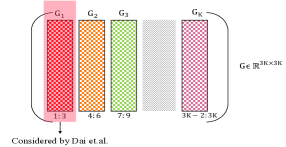
Figure 2: (a) The column triplet (1:3) of euclidean corrective matrix (𝙶𝚔subscript𝙶𝚔\mathchoice{\mbox{\bf$\displaystyle\tt G$}}{\mbox{\bf$\textstyle\tt G$}}{\mbox{\bf$\scriptstyle\tt G$}}{\mbox{\bf$\scriptscriptstyle\tt G$}}_{\mathchoice{\mbox{\bf$\displaystyle\tt k$}}{\mbox{\bf$\textstyle\tt k$}}{\mbox{\bf$\scriptstyle\tt k$}}{\mbox{\bf$\scriptscriptstyle\tt k$}}}) used by Dai et al. work [9] shown in red shade. It is stated with the notion that there is no loss of generality to choose 𝙶1subscript𝙶1\mathchoice{\mbox{\bf$\displaystyle\tt G$}}{\mbox{\bf$\textstyle\tt G$}}{\mbox{\bf$\scriptstyle\tt G$}}{\mbox{\bf$\scriptscriptstyle\tt G$}}_{1}. However, choosing other column triplet may result in better rotation and shape estimate as shown in Figure 4(a) and 4(b)

Dai et al. solution to rotation: They proposed that once the 𝚀𝚔subscript𝚀𝚔\mathchoice{\mbox{\bf$\displaystyle\tt Q$}}{\mbox{\bf$\textstyle\tt Q$}}{\mbox{\bf$\scriptstyle\tt Q$}}{\mbox{\bf$\scriptscriptstyle\tt Q$}}_{\mathchoice{\mbox{\bf$\displaystyle\tt k$}}{\mbox{\bf$\textstyle\tt k$}}{\mbox{\bf$\scriptstyle\tt k$}}{\mbox{\bf$\scriptscriptstyle\tt k$}}} is solved, rather than solving for full Euclidean corrective matrix 𝙶3𝙺×3𝙺𝙶superscript3𝙺3𝙺\mathchoice{\mbox{\bf$\displaystyle\tt G$}}{\mbox{\bf$\textstyle\tt G$}}{\mbox{\bf$\scriptstyle\tt G$}}{\mbox{\bf$\scriptscriptstyle\tt G$}}\in\mathbb{R}^{3\mathchoice{\mbox{\bf$\displaystyle\tt K$}}{\mbox{\bf$\textstyle\tt K$}}{\mbox{\bf$\scriptstyle\tt K$}}{\mbox{\bf$\scriptscriptstyle\tt K$}}\times 3\mathchoice{\mbox{\bf$\displaystyle\tt K$}}{\mbox{\bf$\textstyle\tt K$}}{\mbox{\bf$\scriptstyle\tt K$}}{\mbox{\bf$\scriptscriptstyle\tt K$}}}, use svd() to extract rank 3 𝙶𝚔subscript𝙶𝚔\mathchoice{\mbox{\bf$\displaystyle\tt G$}}{\mbox{\bf$\textstyle\tt G$}}{\mbox{\bf$\scriptstyle\tt G$}}{\mbox{\bf$\scriptscriptstyle\tt G$}}_{\mathchoice{\mbox{\bf$\displaystyle\tt k$}}{\mbox{\bf$\textstyle\tt k$}}{\mbox{\bf$\scriptstyle\tt k$}}{\mbox{\bf$\scriptscriptstyle\tt k$}}}. The solved 𝙶𝚔3𝙺×3subscript𝙶𝚔superscript3𝙺3\mathchoice{\mbox{\bf$\displaystyle\tt G$}}{\mbox{\bf$\textstyle\tt G$}}{\mbox{\bf$\scriptstyle\tt G$}}{\mbox{\bf$\scriptscriptstyle\tt G$}}_{\mathchoice{\mbox{\bf$\displaystyle\tt k$}}{\mbox{\bf$\textstyle\tt k$}}{\mbox{\bf$\scriptstyle\tt k$}}{\mbox{\bf$\scriptscriptstyle\tt k$}}}\in\mathbb{R}^{3\mathchoice{\mbox{\bf$\displaystyle\tt K$}}{\mbox{\bf$\textstyle\tt K$}}{\mbox{\bf$\scriptstyle\tt K$}}{\mbox{\bf$\scriptscriptstyle\tt K$}}\times 3} can then be use to find 𝚁𝚁\textstyle\tt R (Eq:4) up to sign (𝚌iksubscript𝚌ik\mathchoice{\mbox{\bf$\displaystyle\tt c$}}{\mbox{\bf$\textstyle\tt c$}}{\mbox{\bf$\scriptstyle\tt c$}}{\mbox{\bf$\scriptscriptstyle\tt c$}}_{\textrm{ik}}). The method quote “we adopt a simpler approach that directly computes the camera motion 𝚁𝚁\textstyle\tt R from single column-triplet 𝙶𝚔subscript𝙶𝚔\mathchoice{\mbox{\bf$\displaystyle\tt G$}}{\mbox{\bf$\textstyle\tt G$}}{\mbox{\bf$\scriptstyle\tt G$}}{\mbox{\bf$\scriptscriptstyle\tt G$}}_{\mathchoice{\mbox{\bf$\displaystyle\tt k$}}{\mbox{\bf$\textstyle\tt k$}}{\mbox{\bf$\scriptstyle\tt k$}}{\mbox{\bf$\scriptscriptstyle\tt k$}}} without need to fill in a big and full 𝙶𝙶\textstyle\tt G matrix”. Naturally, this single column-triplet is chosen to be the first column-triplet (𝙶1)subscript𝙶1(\mathchoice{\mbox{\bf$\displaystyle\tt G$}}{\mbox{\bf$\textstyle\tt G$}}{\mbox{\bf$\scriptstyle\tt G$}}{\mbox{\bf$\scriptscriptstyle\tt G$}}_{1}) of the 𝙶𝙶\textstyle\tt G matrix (see Fig:2(a)). Now, such strategy give rise to few legitimate concerns

  1. (a)

    When each column triplet {𝙶𝚒}𝚒=1𝙺superscriptsubscriptsubscript𝙶𝚒𝚒1𝙺\{\mathchoice{\mbox{\bf$\displaystyle\tt G$}}{\mbox{\bf$\textstyle\tt G$}}{\mbox{\bf$\scriptstyle\tt G$}}{\mbox{\bf$\scriptscriptstyle\tt G$}}_{\mathchoice{\mbox{\bf$\displaystyle\tt i$}}{\mbox{\bf$\textstyle\tt i$}}{\mbox{\bf$\scriptstyle\tt i$}}{\mbox{\bf$\scriptscriptstyle\tt i$}}}\}_{\mathchoice{\mbox{\bf$\displaystyle\tt i$}}{\mbox{\bf$\textstyle\tt i$}}{\mbox{\bf$\scriptstyle\tt i$}}{\mbox{\bf$\scriptscriptstyle\tt i$}}=1}^{\mathchoice{\mbox{\bf$\displaystyle\tt K$}}{\mbox{\bf$\textstyle\tt K$}}{\mbox{\bf$\scriptstyle\tt K$}}{\mbox{\bf$\scriptscriptstyle\tt K$}}} qualifies for a suitable correction matrix, then why 𝙶1subscript𝙶1\mathchoice{\mbox{\bf$\displaystyle\tt G$}}{\mbox{\bf$\textstyle\tt G$}}{\mbox{\bf$\scriptstyle\tt G$}}{\mbox{\bf$\scriptscriptstyle\tt G$}}_{1} has a high preference? Are we loosing useful information by such unwarranted preference?

  2. (b)

    Will each {𝙶𝚒}𝚒=1𝙺superscriptsubscriptsubscript𝙶𝚒𝚒1𝙺\{\mathchoice{\mbox{\bf$\displaystyle\tt G$}}{\mbox{\bf$\textstyle\tt G$}}{\mbox{\bf$\scriptstyle\tt G$}}{\mbox{\bf$\scriptscriptstyle\tt G$}}_{\mathchoice{\mbox{\bf$\displaystyle\tt i$}}{\mbox{\bf$\textstyle\tt i$}}{\mbox{\bf$\scriptstyle\tt i$}}{\mbox{\bf$\scriptscriptstyle\tt i$}}}\}_{\mathchoice{\mbox{\bf$\displaystyle\tt i$}}{\mbox{\bf$\textstyle\tt i$}}{\mbox{\bf$\scriptstyle\tt i$}}{\mbox{\bf$\scriptscriptstyle\tt i$}}=1}^{\mathchoice{\mbox{\bf$\displaystyle\tt K$}}{\mbox{\bf$\textstyle\tt K$}}{\mbox{\bf$\scriptstyle\tt K$}}{\mbox{\bf$\scriptscriptstyle\tt K$}}} provide the same solution to the rotation matrix?

  3. (c)

    Generally, most real world deformations are smooth in nature [27]. Whether such solution to rotation is good enough for the smooth deformation assumption?

Dai et al. overlooked all these intrinsic issues to solve rotation using their proposed intersection theorem.

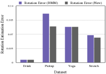
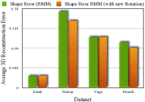
Plausible Rectification: Our experiments show that Dai et al. [9] solution to rotation estimation actually aborted the useful information present in the 𝙶3𝙺×3𝙺𝙶superscript3𝙺3𝙺\mathchoice{\mbox{\bf$\displaystyle\tt G$}}{\mbox{\bf$\textstyle\tt G$}}{\mbox{\bf$\scriptstyle\tt G$}}{\mbox{\bf$\scriptscriptstyle\tt G$}}\in\mathbb{R}^{3\mathchoice{\mbox{\bf$\displaystyle\tt K$}}{\mbox{\bf$\textstyle\tt K$}}{\mbox{\bf$\scriptstyle\tt K$}}{\mbox{\bf$\scriptscriptstyle\tt K$}}\times 3\mathchoice{\mbox{\bf$\displaystyle\tt K$}}{\mbox{\bf$\textstyle\tt K$}}{\mbox{\bf$\scriptstyle\tt K$}}{\mbox{\bf$\scriptscriptstyle\tt K$}}}. Each of the ‘𝙺𝙺\textstyle\tt K’ column triplets in 𝙶𝙶\textstyle\tt G (i.e. 𝙶𝚔subscript𝙶𝚔\mathchoice{\mbox{\bf$\displaystyle\tt G$}}{\mbox{\bf$\textstyle\tt G$}}{\mbox{\bf$\scriptstyle\tt G$}}{\mbox{\bf$\scriptscriptstyle\tt G$}}_{\mathchoice{\mbox{\bf$\displaystyle\tt k$}}{\mbox{\bf$\textstyle\tt k$}}{\mbox{\bf$\scriptstyle\tt k$}}{\mbox{\bf$\scriptscriptstyle\tt k$}}}) gives a possible rotation matrix which is different from each other (see Fig:(3)). Our empirical evaluations on several datasets show that the first column triplet is not always the best choice to estimate rotation. Hence, the details provided by Dai et al. work [9] is incomplete and there is a loss of generality with such procedure to estimate rotation under the well-known assumption of smooth deformation [27]. Fig:(4(a)) and Fig:(4(b)) provides few statistical results with comparison for both rotation and shape error estimate respectively. For clarity, we also provide the column triplet index that gives the better results for the corresponding data sequence and therefore, provides few counter-examples to such generalization.

Refer to caption
(a) 𝚁𝙶1𝚁subscript𝙶1\mathchoice{\mbox{\bf$\displaystyle\tt R$}}{\mbox{\bf$\textstyle\tt R$}}{\mbox{\bf$\scriptstyle\tt R$}}{\mbox{\bf$\scriptscriptstyle\tt R$}}\leftarrow\mathchoice{\mbox{\bf$\displaystyle\tt G$}}{\mbox{\bf$\textstyle\tt G$}}{\mbox{\bf$\scriptstyle\tt G$}}{\mbox{\bf$\scriptscriptstyle\tt G$}}_{1}
Refer to caption
(b) 𝚁𝙶2𝚁subscript𝙶2\mathchoice{\mbox{\bf$\displaystyle\tt R$}}{\mbox{\bf$\textstyle\tt R$}}{\mbox{\bf$\scriptstyle\tt R$}}{\mbox{\bf$\scriptscriptstyle\tt R$}}\leftarrow\mathchoice{\mbox{\bf$\displaystyle\tt G$}}{\mbox{\bf$\textstyle\tt G$}}{\mbox{\bf$\scriptstyle\tt G$}}{\mbox{\bf$\scriptscriptstyle\tt G$}}_{2}
Refer to caption
(c) 𝚁𝙶3𝚁subscript𝙶3\mathchoice{\mbox{\bf$\displaystyle\tt R$}}{\mbox{\bf$\textstyle\tt R$}}{\mbox{\bf$\scriptstyle\tt R$}}{\mbox{\bf$\scriptscriptstyle\tt R$}}\leftarrow\mathchoice{\mbox{\bf$\displaystyle\tt G$}}{\mbox{\bf$\textstyle\tt G$}}{\mbox{\bf$\scriptstyle\tt G$}}{\mbox{\bf$\scriptscriptstyle\tt G$}}_{3}
Refer to caption
(d) 𝚁𝙶4𝚁subscript𝙶4\mathchoice{\mbox{\bf$\displaystyle\tt R$}}{\mbox{\bf$\textstyle\tt R$}}{\mbox{\bf$\scriptstyle\tt R$}}{\mbox{\bf$\scriptscriptstyle\tt R$}}\leftarrow\mathchoice{\mbox{\bf$\displaystyle\tt G$}}{\mbox{\bf$\textstyle\tt G$}}{\mbox{\bf$\scriptstyle\tt G$}}{\mbox{\bf$\scriptscriptstyle\tt G$}}_{4}
Refer to caption
(e) 𝚁𝙶5𝚁subscript𝙶5\mathchoice{\mbox{\bf$\displaystyle\tt R$}}{\mbox{\bf$\textstyle\tt R$}}{\mbox{\bf$\scriptstyle\tt R$}}{\mbox{\bf$\scriptscriptstyle\tt R$}}\leftarrow\mathchoice{\mbox{\bf$\displaystyle\tt G$}}{\mbox{\bf$\textstyle\tt G$}}{\mbox{\bf$\scriptstyle\tt G$}}{\mbox{\bf$\scriptscriptstyle\tt G$}}_{5}
Refer to caption
(f) 𝚁𝙶6𝚁subscript𝙶6\mathchoice{\mbox{\bf$\displaystyle\tt R$}}{\mbox{\bf$\textstyle\tt R$}}{\mbox{\bf$\scriptstyle\tt R$}}{\mbox{\bf$\scriptscriptstyle\tt R$}}\leftarrow\mathchoice{\mbox{\bf$\displaystyle\tt G$}}{\mbox{\bf$\textstyle\tt G$}}{\mbox{\bf$\scriptstyle\tt G$}}{\mbox{\bf$\scriptscriptstyle\tt G$}}_{6}
Refer to caption
(g) 𝚁𝙶7𝚁subscript𝙶7\mathchoice{\mbox{\bf$\displaystyle\tt R$}}{\mbox{\bf$\textstyle\tt R$}}{\mbox{\bf$\scriptstyle\tt R$}}{\mbox{\bf$\scriptscriptstyle\tt R$}}\leftarrow\mathchoice{\mbox{\bf$\displaystyle\tt G$}}{\mbox{\bf$\textstyle\tt G$}}{\mbox{\bf$\scriptstyle\tt G$}}{\mbox{\bf$\scriptscriptstyle\tt G$}}_{7}
Refer to caption
(h) 𝚁𝙶8𝚁subscript𝙶8\mathchoice{\mbox{\bf$\displaystyle\tt R$}}{\mbox{\bf$\textstyle\tt R$}}{\mbox{\bf$\scriptstyle\tt R$}}{\mbox{\bf$\scriptscriptstyle\tt R$}}\leftarrow\mathchoice{\mbox{\bf$\displaystyle\tt G$}}{\mbox{\bf$\textstyle\tt G$}}{\mbox{\bf$\scriptstyle\tt G$}}{\mbox{\bf$\scriptscriptstyle\tt G$}}_{8}
Refer to caption
(i) 𝚁𝙶9𝚁subscript𝙶9\mathchoice{\mbox{\bf$\displaystyle\tt R$}}{\mbox{\bf$\textstyle\tt R$}}{\mbox{\bf$\scriptstyle\tt R$}}{\mbox{\bf$\scriptscriptstyle\tt R$}}\leftarrow\mathchoice{\mbox{\bf$\displaystyle\tt G$}}{\mbox{\bf$\textstyle\tt G$}}{\mbox{\bf$\scriptstyle\tt G$}}{\mbox{\bf$\scriptscriptstyle\tt G$}}_{9}
Refer to caption
(j) 𝚁𝙶10𝚁subscript𝙶10\mathchoice{\mbox{\bf$\displaystyle\tt R$}}{\mbox{\bf$\textstyle\tt R$}}{\mbox{\bf$\scriptstyle\tt R$}}{\mbox{\bf$\scriptscriptstyle\tt R$}}\leftarrow\mathchoice{\mbox{\bf$\displaystyle\tt G$}}{\mbox{\bf$\textstyle\tt G$}}{\mbox{\bf$\scriptstyle\tt G$}}{\mbox{\bf$\scriptscriptstyle\tt G$}}_{10}
Refer to caption
(k) 𝚁𝙶11𝚁subscript𝙶11\mathchoice{\mbox{\bf$\displaystyle\tt R$}}{\mbox{\bf$\textstyle\tt R$}}{\mbox{\bf$\scriptstyle\tt R$}}{\mbox{\bf$\scriptscriptstyle\tt R$}}\leftarrow\mathchoice{\mbox{\bf$\displaystyle\tt G$}}{\mbox{\bf$\textstyle\tt G$}}{\mbox{\bf$\scriptstyle\tt G$}}{\mbox{\bf$\scriptscriptstyle\tt G$}}_{11}
Refer to caption
(l) 𝚁𝙶12𝚁subscript𝙶12\mathchoice{\mbox{\bf$\displaystyle\tt R$}}{\mbox{\bf$\textstyle\tt R$}}{\mbox{\bf$\scriptstyle\tt R$}}{\mbox{\bf$\scriptscriptstyle\tt R$}}\leftarrow\mathchoice{\mbox{\bf$\displaystyle\tt G$}}{\mbox{\bf$\textstyle\tt G$}}{\mbox{\bf$\scriptstyle\tt G$}}{\mbox{\bf$\scriptscriptstyle\tt G$}}_{12}
Figure 3: The rotation samples on 𝕊𝕆(3)𝕊𝕆3\mathbb{SO}(3) using {𝙶𝚔}𝚔=112superscriptsubscriptsubscript𝙶𝚔𝚔112\{\mathchoice{\mbox{\bf$\displaystyle\tt G$}}{\mbox{\bf$\textstyle\tt G$}}{\mbox{\bf$\scriptstyle\tt G$}}{\mbox{\bf$\scriptscriptstyle\tt G$}}_{\mathchoice{\mbox{\bf$\displaystyle\tt k$}}{\mbox{\bf$\textstyle\tt k$}}{\mbox{\bf$\scriptstyle\tt k$}}{\mbox{\bf$\scriptscriptstyle\tt k$}}}\}_{\mathchoice{\mbox{\bf$\displaystyle\tt k$}}{\mbox{\bf$\textstyle\tt k$}}{\mbox{\bf$\scriptstyle\tt k$}}{\mbox{\bf$\scriptscriptstyle\tt k$}}=1}^{12} for Pick-up sequence. Below each 𝕊𝕆(3)𝕊𝕆3\mathbb{SO}(3) manifold is the graph showing the per frame change in the camera motion using Eq:(8) ‘δ𝚏subscript𝛿𝚏\delta_{\mathchoice{\mbox{\bf$\displaystyle\tt f$}}{\mbox{\bf$\textstyle\tt f$}}{\mbox{\bf$\scriptstyle\tt f$}}{\mbox{\bf$\scriptscriptstyle\tt f$}}}’. A simple observation establishes that all rotation matrix (𝚁𝚁\textstyle\tt R) are not the same. ‘δ𝚏subscript𝛿𝚏\delta_{\mathchoice{\mbox{\bf$\displaystyle\tt f$}}{\mbox{\bf$\textstyle\tt f$}}{\mbox{\bf$\scriptstyle\tt f$}}{\mbox{\bf$\scriptscriptstyle\tt f$}}}’ graph analysis on this dataset show that the rotation estimate provided by 𝙶7,𝙶8subscript𝙶7subscript𝙶8\mathchoice{\mbox{\bf$\displaystyle\tt G$}}{\mbox{\bf$\textstyle\tt G$}}{\mbox{\bf$\scriptstyle\tt G$}}{\mbox{\bf$\scriptscriptstyle\tt G$}}_{7},\mathchoice{\mbox{\bf$\displaystyle\tt G$}}{\mbox{\bf$\textstyle\tt G$}}{\mbox{\bf$\scriptstyle\tt G$}}{\mbox{\bf$\scriptscriptstyle\tt G$}}_{8}, 𝙶9subscript𝙶9\mathchoice{\mbox{\bf$\displaystyle\tt G$}}{\mbox{\bf$\textstyle\tt G$}}{\mbox{\bf$\scriptstyle\tt G$}}{\mbox{\bf$\scriptscriptstyle\tt G$}}_{9} has a smoother camera motion than other 𝙶𝚔subscript𝙶𝚔\mathchoice{\mbox{\bf$\displaystyle\tt G$}}{\mbox{\bf$\textstyle\tt G$}}{\mbox{\bf$\scriptstyle\tt G$}}{\mbox{\bf$\scriptscriptstyle\tt G$}}_{\mathchoice{\mbox{\bf$\displaystyle\tt k$}}{\mbox{\bf$\textstyle\tt k$}}{\mbox{\bf$\scriptstyle\tt k$}}{\mbox{\bf$\scriptscriptstyle\tt k$}}}’s, with 𝙶9subscript𝙶9\mathchoice{\mbox{\bf$\displaystyle\tt G$}}{\mbox{\bf$\textstyle\tt G$}}{\mbox{\bf$\scriptstyle\tt G$}}{\mbox{\bf$\scriptscriptstyle\tt G$}}_{9} being the smoothest. Any one out of these 3 𝙶𝚔subscript𝙶𝚔\mathchoice{\mbox{\bf$\displaystyle\tt G$}}{\mbox{\bf$\textstyle\tt G$}}{\mbox{\bf$\scriptstyle\tt G$}}{\mbox{\bf$\scriptscriptstyle\tt G$}}_{\mathchoice{\mbox{\bf$\displaystyle\tt k$}}{\mbox{\bf$\textstyle\tt k$}}{\mbox{\bf$\scriptstyle\tt k$}}{\mbox{\bf$\scriptscriptstyle\tt k$}}}’s supply better performance than 𝙶1subscript𝙶1\mathchoice{\mbox{\bf$\displaystyle\tt G$}}{\mbox{\bf$\textstyle\tt G$}}{\mbox{\bf$\scriptstyle\tt G$}}{\mbox{\bf$\scriptscriptstyle\tt G$}}_{1}. Note: Each 𝚁𝚒2×3𝚁𝚒3×3subscript𝚁𝚒superscript23maps-tosubscript𝚁𝚒superscript33\mathchoice{\mbox{\bf$\displaystyle\tt R$}}{\mbox{\bf$\textstyle\tt R$}}{\mbox{\bf$\scriptstyle\tt R$}}{\mbox{\bf$\scriptscriptstyle\tt R$}}_{\mathchoice{\mbox{\bf$\displaystyle\tt i$}}{\mbox{\bf$\textstyle\tt i$}}{\mbox{\bf$\scriptstyle\tt i$}}{\mbox{\bf$\scriptscriptstyle\tt i$}}}\in\mathbb{R}^{2\times 3}\mapsto\mathchoice{\mbox{\bf$\displaystyle\tt R$}}{\mbox{\bf$\textstyle\tt R$}}{\mbox{\bf$\scriptstyle\tt R$}}{\mbox{\bf$\scriptscriptstyle\tt R$}}_{\mathchoice{\mbox{\bf$\displaystyle\tt i$}}{\mbox{\bf$\textstyle\tt i$}}{\mbox{\bf$\scriptstyle\tt i$}}{\mbox{\bf$\scriptscriptstyle\tt i$}}}\in\mathbb{R}^{3\times 3} via cross product. (Best viewed on screen)

Theoretically and practically, this result is of significant importance as it helps in inferring that the solution provided by “Intersection Theorem" has a lot of useful information left to be exploited completely and Dai et al. work ignored this. Also, it gives rise to some challenges that finding the best column triplet for 𝙶𝚔subscript𝙶𝚔\mathchoice{\mbox{\bf$\displaystyle\tt G$}}{\mbox{\bf$\textstyle\tt G$}}{\mbox{\bf$\scriptstyle\tt G$}}{\mbox{\bf$\scriptscriptstyle\tt G$}}_{\mathchoice{\mbox{\bf$\displaystyle\tt k$}}{\mbox{\bf$\textstyle\tt k$}}{\mbox{\bf$\scriptstyle\tt k$}}{\mbox{\bf$\scriptscriptstyle\tt k$}}} is not an easy task. With these results, we conjecture few problems for further research in NRSfM that are: (a) Can we find a best possible column triplet for the corrective matrix with a given rank prior ‘(𝙺)𝙺(\mathchoice{\mbox{\bf$\displaystyle\tt K$}}{\mbox{\bf$\textstyle\tt K$}}{\mbox{\bf$\scriptstyle\tt K$}}{\mbox{\bf$\scriptscriptstyle\tt K$}})’, or (b) At least can we put an upper bound on the value 𝚔𝙺𝚔𝙺\mathchoice{\mbox{\bf$\displaystyle\tt k$}}{\mbox{\bf$\textstyle\tt k$}}{\mbox{\bf$\scriptstyle\tt k$}}{\mbox{\bf$\scriptscriptstyle\tt k$}}\subset\mathchoice{\mbox{\bf$\displaystyle\tt K$}}{\mbox{\bf$\textstyle\tt K$}}{\mbox{\bf$\scriptstyle\tt K$}}{\mbox{\bf$\scriptscriptstyle\tt K$}} such that there exists no such ‘𝚔𝚔\textstyle\tt k’ for 𝙶𝚔subscript𝙶𝚔\mathchoice{\mbox{\bf$\displaystyle\tt G$}}{\mbox{\bf$\textstyle\tt G$}}{\mbox{\bf$\scriptstyle\tt G$}}{\mbox{\bf$\scriptscriptstyle\tt G$}}_{\mathchoice{\mbox{\bf$\displaystyle\tt k$}}{\mbox{\bf$\textstyle\tt k$}}{\mbox{\bf$\scriptstyle\tt k$}}{\mbox{\bf$\scriptscriptstyle\tt k$}}} which will provide better rotation and structure estimate. The problem seems hard keeping in view that the prior rank (𝙺)𝙺(\mathchoice{\mbox{\bf$\displaystyle\tt K$}}{\mbox{\bf$\textstyle\tt K$}}{\mbox{\bf$\scriptstyle\tt K$}}{\mbox{\bf$\scriptscriptstyle\tt K$}}) in NRSfM factorization methods is an assumed approximation and it changes for different datasets to achieve better results.
A solution: In 2005, Brand. M [4] argued to use full correction matrix to estimate motion which in a way utilizes all the multiple estimates of column-triads of 𝙶𝙶\textstyle\tt G. Recently, Lee et al. [23] briefly mentions on the problems with motion estimates using [9]. In contrast, we use an analytical observation based on the smoothness and regularity222The term <<regularity>> is used in a loose sense (Mathematically). of the camera motion trajectory to filter 𝙶𝚔3𝙺×3subscript𝙶𝚔superscript3𝙺3\mathchoice{\mbox{\bf$\displaystyle\tt G$}}{\mbox{\bf$\textstyle\tt G$}}{\mbox{\bf$\scriptstyle\tt G$}}{\mbox{\bf$\scriptscriptstyle\tt G$}}_{\mathchoice{\mbox{\bf$\displaystyle\tt k$}}{\mbox{\bf$\textstyle\tt k$}}{\mbox{\bf$\scriptstyle\tt k$}}{\mbox{\bf$\scriptscriptstyle\tt k$}}}\in\mathbb{R}^{3\mathchoice{\mbox{\bf$\displaystyle\tt K$}}{\mbox{\bf$\textstyle\tt K$}}{\mbox{\bf$\scriptstyle\tt K$}}{\mbox{\bf$\scriptscriptstyle\tt K$}}\times 3} to infer better ‘𝚁𝚁\textstyle\tt R’. Let ψ(.)\psi(.) be a function that takes 𝙶𝚔subscript𝙶𝚔\mathchoice{\mbox{\bf$\displaystyle\tt G$}}{\mbox{\bf$\textstyle\tt G$}}{\mbox{\bf$\scriptstyle\tt G$}}{\mbox{\bf$\scriptscriptstyle\tt G$}}_{\mathchoice{\mbox{\bf$\displaystyle\tt k$}}{\mbox{\bf$\textstyle\tt k$}}{\mbox{\bf$\scriptstyle\tt k$}}{\mbox{\bf$\scriptscriptstyle\tt k$}}} as input and gives ‘𝚁𝚁\textstyle\tt R’ as output using Intersection theorem. We estimate different 𝚁2𝙵×3𝙵𝚁superscript2𝙵3𝙵\mathchoice{\mbox{\bf$\displaystyle\tt R$}}{\mbox{\bf$\textstyle\tt R$}}{\mbox{\bf$\scriptstyle\tt R$}}{\mbox{\bf$\scriptscriptstyle\tt R$}}\in\mathbb{R}^{2\mathchoice{\mbox{\bf$\displaystyle\tt F$}}{\mbox{\bf$\textstyle\tt F$}}{\mbox{\bf$\scriptstyle\tt F$}}{\mbox{\bf$\scriptscriptstyle\tt F$}}\times 3\mathchoice{\mbox{\bf$\displaystyle\tt F$}}{\mbox{\bf$\textstyle\tt F$}}{\mbox{\bf$\scriptstyle\tt F$}}{\mbox{\bf$\scriptscriptstyle\tt F$}}} for all the column triplets {𝙶𝚔}𝚔=1𝙺superscriptsubscriptsubscript𝙶𝚔𝚔1𝙺\{\mathchoice{\mbox{\bf$\displaystyle\tt G$}}{\mbox{\bf$\textstyle\tt G$}}{\mbox{\bf$\scriptstyle\tt G$}}{\mbox{\bf$\scriptscriptstyle\tt G$}}_{\mathchoice{\mbox{\bf$\displaystyle\tt k$}}{\mbox{\bf$\textstyle\tt k$}}{\mbox{\bf$\scriptstyle\tt k$}}{\mbox{\bf$\scriptscriptstyle\tt k$}}}\}_{\mathchoice{\mbox{\bf$\displaystyle\tt k$}}{\mbox{\bf$\textstyle\tt k$}}{\mbox{\bf$\scriptstyle\tt k$}}{\mbox{\bf$\scriptscriptstyle\tt k$}}=1}^{\mathchoice{\mbox{\bf$\displaystyle\tt K$}}{\mbox{\bf$\textstyle\tt K$}}{\mbox{\bf$\scriptstyle\tt K$}}{\mbox{\bf$\scriptscriptstyle\tt K$}}}, then compute smoothness of the camera motion for each 𝙶𝚔subscript𝙶𝚔\mathchoice{\mbox{\bf$\displaystyle\tt G$}}{\mbox{\bf$\textstyle\tt G$}}{\mbox{\bf$\scriptstyle\tt G$}}{\mbox{\bf$\scriptscriptstyle\tt G$}}_{\mathchoice{\mbox{\bf$\displaystyle\tt k$}}{\mbox{\bf$\textstyle\tt k$}}{\mbox{\bf$\scriptstyle\tt k$}}{\mbox{\bf$\scriptscriptstyle\tt k$}}} as:

Suppose,𝚁=ψ(𝙶𝚔),via Intersection method, then,Suppose,𝚁𝜓subscript𝙶𝚔via Intersection method, then,\displaystyle\textrm{Suppose,}~{}\mathchoice{\mbox{\bf$\displaystyle\tt R$}}{\mbox{\bf$\textstyle\tt R$}}{\mbox{\bf$\scriptstyle\tt R$}}{\mbox{\bf$\scriptscriptstyle\tt R$}}=\psi(\mathchoice{\mbox{\bf$\displaystyle\tt G$}}{\mbox{\bf$\textstyle\tt G$}}{\mbox{\bf$\scriptstyle\tt G$}}{\mbox{\bf$\scriptscriptstyle\tt G$}}_{\mathchoice{\mbox{\bf$\displaystyle\tt k$}}{\mbox{\bf$\textstyle\tt k$}}{\mbox{\bf$\scriptstyle\tt k$}}{\mbox{\bf$\scriptscriptstyle\tt k$}}}),~{}\textrm{via Intersection method, then, } (8)
δ𝚏=𝚁𝚏𝚁𝚏+1𝙵2𝚏=1,2,,𝙵1.[13]Sec.4.formulae-sequencesubscript𝛿𝚏superscriptsubscriptnormsubscript𝚁𝚏subscript𝚁𝚏1𝙵2for-all𝚏12𝙵1[13]Sec.4\displaystyle\delta_{\mathchoice{\mbox{\bf$\displaystyle\tt f$}}{\mbox{\bf$\textstyle\tt f$}}{\mbox{\bf$\scriptstyle\tt f$}}{\mbox{\bf$\scriptscriptstyle\tt f$}}}=\|\mathchoice{\mbox{\bf$\displaystyle\tt R$}}{\mbox{\bf$\textstyle\tt R$}}{\mbox{\bf$\scriptstyle\tt R$}}{\mbox{\bf$\scriptscriptstyle\tt R$}}_{\mathchoice{\mbox{\bf$\displaystyle\tt f$}}{\mbox{\bf$\textstyle\tt f$}}{\mbox{\bf$\scriptstyle\tt f$}}{\mbox{\bf$\scriptscriptstyle\tt f$}}}-\mathchoice{\mbox{\bf$\displaystyle\tt R$}}{\mbox{\bf$\textstyle\tt R$}}{\mbox{\bf$\scriptstyle\tt R$}}{\mbox{\bf$\scriptscriptstyle\tt R$}}_{\mathchoice{\mbox{\bf$\displaystyle\tt f$}}{\mbox{\bf$\textstyle\tt f$}}{\mbox{\bf$\scriptstyle\tt f$}}{\mbox{\bf$\scriptscriptstyle\tt f$}}+1}\|_{\mathchoice{\mbox{\bf$\displaystyle\tt F$}}{\mbox{\bf$\textstyle\tt F$}}{\mbox{\bf$\scriptstyle\tt F$}}{\mbox{\bf$\scriptscriptstyle\tt F$}}}^{2}~{}~{}\forall~{}\mathchoice{\mbox{\bf$\displaystyle\tt f$}}{\mbox{\bf$\textstyle\tt f$}}{\mbox{\bf$\scriptstyle\tt f$}}{\mbox{\bf$\scriptscriptstyle\tt f$}}=1,2,...,\mathchoice{\mbox{\bf$\displaystyle\tt F$}}{\mbox{\bf$\textstyle\tt F$}}{\mbox{\bf$\scriptstyle\tt F$}}{\mbox{\bf$\scriptscriptstyle\tt F$}}-1.~{}\cite[cite]{[\@@bibref{}{hartley2013rotation}{}{}]}~{}\textrm{Sec.{\bf{4}}}.

By examining the smoothness of the camera motion for each 𝙶𝚔subscript𝙶𝚔\mathchoice{\mbox{\bf$\displaystyle\tt G$}}{\mbox{\bf$\textstyle\tt G$}}{\mbox{\bf$\scriptstyle\tt G$}}{\mbox{\bf$\scriptscriptstyle\tt G$}}_{\mathchoice{\mbox{\bf$\displaystyle\tt k$}}{\mbox{\bf$\textstyle\tt k$}}{\mbox{\bf$\scriptstyle\tt k$}}{\mbox{\bf$\scriptscriptstyle\tt k$}}}, we select the suitable rotation matrix for structure estimation (see Fig. 3). Our strategy to select smooth camera motion over frames based on Eq:(8) consistently supplied us with better performance than the previously proposed approach. We acknowledge that this is not a profound way to infer the best rotation, however, it does provide a possibility to deduce better rotation using “prior-free" approach which respects the well-known assumption of smooth deformation in NRSfM. Further, it helps endorse our claim on the generalization of rotation estimate by [9]. You may use the variable ‘δ𝚏subscript𝛿𝚏\delta_{\mathchoice{\mbox{\bf$\displaystyle\tt f$}}{\mbox{\bf$\textstyle\tt f$}}{\mbox{\bf$\scriptstyle\tt f$}}{\mbox{\bf$\scriptscriptstyle\tt f$}}}’ Eq:(8) as a smoothness term in the final optimization (Eq:(11)) to further improve rotation, however, to show the competence within the “prior-free” idea [9], we stick to the classical two staged approach.
Refer to caption
(a)
Refer to caption
(b)
Figure 4: Counter examples on benchmark dataset [2]. (a) Rotation error in comparison to BMM [9] on synthetic data. (b) 3D reconstruction error using global trace norm minimization of shape matrix as used in BMM with rotation matrix estimate using other column triplet in comparison to 𝙶𝙶\textstyle\tt G(1:3). The column triplets of (𝙶𝙶\textstyle\tt G) for which the method perform better on Drink, Pickup, Yoga and Stretch are (1:3), (19:21), (1:3) and (19:21) respectively. Note that we used the same rank prior value ‘𝙺𝙺\textstyle\tt K’ used in Dai et al. work [9].

3 Structure Estimation

Once the rotation is estimated based on the smoothness of the camera motion [27], the next step is to solve for 3D structure. The block matrix method (BMM) by Dai et al. [9] proposed the following optimization problem to estimate the non-rigid low-rank shape.

minimize𝚂𝚂subject to:𝚆=𝚁𝚂,𝚂=g(𝚂)formulae-sequencesuperscript𝚂minimizesubscriptnormsuperscript𝚂subject to:𝚆𝚁𝚂superscript𝚂𝑔𝚂\displaystyle\underset{\mathchoice{\mbox{\bf$\displaystyle\tt S$}}{\mbox{\bf$\textstyle\tt S$}}{\mbox{\bf$\scriptstyle\tt S$}}{\mbox{\bf$\scriptscriptstyle\tt S$}}^{\sharp}}{{\text{minimize}}}~{}\|\mathchoice{\mbox{\bf$\displaystyle\tt S$}}{\mbox{\bf$\textstyle\tt S$}}{\mbox{\bf$\scriptstyle\tt S$}}{\mbox{\bf$\scriptscriptstyle\tt S$}}^{\sharp}\|_{*}{~{}\text{subject to:}}~{}\mathchoice{\mbox{\bf$\displaystyle\tt W$}}{\mbox{\bf$\textstyle\tt W$}}{\mbox{\bf$\scriptstyle\tt W$}}{\mbox{\bf$\scriptscriptstyle\tt W$}}=\mathchoice{\mbox{\bf$\displaystyle\tt R$}}{\mbox{\bf$\textstyle\tt R$}}{\mbox{\bf$\scriptstyle\tt R$}}{\mbox{\bf$\scriptscriptstyle\tt R$}}\mathchoice{\mbox{\bf$\displaystyle\tt S$}}{\mbox{\bf$\textstyle\tt S$}}{\mbox{\bf$\scriptstyle\tt S$}}{\mbox{\bf$\scriptscriptstyle\tt S$}},\mathchoice{\mbox{\bf$\displaystyle\tt S$}}{\mbox{\bf$\textstyle\tt S$}}{\mbox{\bf$\scriptstyle\tt S$}}{\mbox{\bf$\scriptscriptstyle\tt S$}}^{\sharp}=g(\mathchoice{\mbox{\bf$\displaystyle\tt S$}}{\mbox{\bf$\textstyle\tt S$}}{\mbox{\bf$\scriptstyle\tt S$}}{\mbox{\bf$\scriptscriptstyle\tt S$}}) (9)

where, 𝚂𝙵×𝟹𝙿superscript𝚂superscript𝙵𝟹𝙿\mathchoice{\mbox{\bf$\displaystyle\tt S$}}{\mbox{\bf$\textstyle\tt S$}}{\mbox{\bf$\scriptstyle\tt S$}}{\mbox{\bf$\scriptscriptstyle\tt S$}}^{\sharp}\in\mathbb{R}^{\mathchoice{\mbox{\bf$\displaystyle\tt F$}}{\mbox{\bf$\textstyle\tt F$}}{\mbox{\bf$\scriptstyle\tt F$}}{\mbox{\bf$\scriptscriptstyle\tt F$}}\times\mathchoice{\mbox{\bf$\displaystyle\tt 3$}}{\mbox{\bf$\textstyle\tt 3$}}{\mbox{\bf$\scriptstyle\tt 3$}}{\mbox{\bf$\scriptscriptstyle\tt 3$}}\mathchoice{\mbox{\bf$\displaystyle\tt P$}}{\mbox{\bf$\textstyle\tt P$}}{\mbox{\bf$\scriptstyle\tt P$}}{\mbox{\bf$\scriptscriptstyle\tt P$}}} is a rearranged shape matrix with each row corresponds to the shape for that frame. The trace norm minimization on ‘𝚂superscript𝚂\mathchoice{\mbox{\bf$\displaystyle\tt S$}}{\mbox{\bf$\textstyle\tt S$}}{\mbox{\bf$\scriptstyle\tt S$}}{\mbox{\bf$\scriptscriptstyle\tt S$}}^{\sharp}’ is enforced instead of ‘𝚂𝚂\textstyle\tt S’ to provide a stronger rank bound on the shape matrix [9]. The second term in Eq:(9) enforces the re-projection error constraint. The function g(.)g(.) maps 𝚂3𝙵×𝙿𝚂superscript3𝙵𝙿\mathchoice{\mbox{\bf$\displaystyle\tt S$}}{\mbox{\bf$\textstyle\tt S$}}{\mbox{\bf$\scriptstyle\tt S$}}{\mbox{\bf$\scriptscriptstyle\tt S$}}\in\mathbb{R}^{3\mathchoice{\mbox{\bf$\displaystyle\tt F$}}{\mbox{\bf$\textstyle\tt F$}}{\mbox{\bf$\scriptstyle\tt F$}}{\mbox{\bf$\scriptscriptstyle\tt F$}}\times\mathchoice{\mbox{\bf$\displaystyle\tt P$}}{\mbox{\bf$\textstyle\tt P$}}{\mbox{\bf$\scriptstyle\tt P$}}{\mbox{\bf$\scriptscriptstyle\tt P$}}} to 𝚂𝙵×3𝙿superscript𝚂superscript𝙵3𝙿\mathchoice{\mbox{\bf$\displaystyle\tt S$}}{\mbox{\bf$\textstyle\tt S$}}{\mbox{\bf$\scriptstyle\tt S$}}{\mbox{\bf$\scriptscriptstyle\tt S$}}^{\sharp}\in\mathbb{R}^{\mathchoice{\mbox{\bf$\displaystyle\tt F$}}{\mbox{\bf$\textstyle\tt F$}}{\mbox{\bf$\scriptstyle\tt F$}}{\mbox{\bf$\scriptscriptstyle\tt F$}}\times 3\mathchoice{\mbox{\bf$\displaystyle\tt P$}}{\mbox{\bf$\textstyle\tt P$}}{\mbox{\bf$\scriptstyle\tt P$}}{\mbox{\bf$\scriptscriptstyle\tt P$}}}.

Dai et al. solution to shape: Following the work of Ma et al. [26] on rank minimization problems, Dai et al. [9] proposed a solution to the optimization in Eq:(9). The method enforces low-rank constraint on ‘𝚂superscript𝚂\mathchoice{\mbox{\bf$\displaystyle\tt S$}}{\mbox{\bf$\textstyle\tt S$}}{\mbox{\bf$\scriptstyle\tt S$}}{\mbox{\bf$\scriptscriptstyle\tt S$}}^{\sharp}’ matrix and provide the solution by solving Eq:(9) via ADMM[3] using matrix shrinkage operator 𝒮λ(𝚇)subscript𝒮𝜆𝚇\mathcal{S}_{\lambda}(\mathchoice{\mbox{\bf$\displaystyle\tt X$}}{\mbox{\bf$\textstyle\tt X$}}{\mbox{\bf$\scriptstyle\tt X$}}{\mbox{\bf$\scriptscriptstyle\tt X$}}) = 𝚄diag(sλ(σ))𝚅𝚃𝚄diagsubscript𝑠𝜆𝜎superscript𝚅𝚃\mathchoice{\mbox{\bf$\displaystyle\tt U$}}{\mbox{\bf$\textstyle\tt U$}}{\mbox{\bf$\scriptstyle\tt U$}}{\mbox{\bf$\scriptscriptstyle\tt U$}}\text{diag}(s_{\lambda}(\sigma))\mathchoice{\mbox{\bf$\displaystyle\tt V$}}{\mbox{\bf$\textstyle\tt V$}}{\mbox{\bf$\scriptstyle\tt V$}}{\mbox{\bf$\scriptscriptstyle\tt V$}}^{\mathchoice{\mbox{\bf$\displaystyle\tt T$}}{\mbox{\bf$\textstyle\tt T$}}{\mbox{\bf$\scriptstyle\tt T$}}{\mbox{\bf$\scriptscriptstyle\tt T$}}}, where sλ(σ)subscript𝑠𝜆𝜎s_{\lambda}(\sigma) = σ¯¯𝜎\bar{\sigma} with σi¯¯subscript𝜎𝑖\bar{\sigma_{i}} = {σiλifσiλ>0\big{\{}\sigma_{i}-\lambda~{}\text{if}~{}\sigma_{i}-\lambda>0 and 0 otherwise }.

Plausible Rectification: Despite the trace norm minimization provides a satisfactory solution to non-rigid structure estimation, it has some serious issues. The proposed solution to nuclear norm minimization problem (Eq:(9)) gives equal priority to each singular values, as a result, the shrinkage operator penalizes each singular value with the same quantity (λ𝜆\lambda). To estimate 3D structure of a non-rigidly deforming object using matrix factorization approach, we use a prior assumption that the shape lies in a low-rank subspace. Therefore, it’s not a better choice to penalize the major component of the shape data and its very minor component equally. Consequently, nuclear norm minimization of the shape matrix struggles to appropriately conserve the useful component of the non-rigidly deforming shape.

Truncated nuclear norm regularization can be a choice to handle such issues, however, it depends on the binary decision, hence not versatile in nature [35]. To really cater the behavior of the deformations based on its low-rank nature, we propose to use weighted nuclear norm minimization approach to solve for non-rigid structure [28, 12]. In contrast to the previous notation to the nuclear norm of the shape matrix i.e. 𝚂subscriptnormsuperscript𝚂\|\mathchoice{\mbox{\bf$\displaystyle\tt S$}}{\mbox{\bf$\textstyle\tt S$}}{\mbox{\bf$\scriptstyle\tt S$}}{\mbox{\bf$\scriptscriptstyle\tt S$}}^{\sharp}\|_{*}, we introduce a different notation for its weighted nuclear norm

𝚂Θ,=𝚓=1𝙺Θ𝚓σ𝚓(𝚂)subscriptnormsuperscript𝚂Θsuperscriptsubscript𝚓1𝙺subscriptΘ𝚓subscript𝜎𝚓superscript𝚂\|\mathchoice{\mbox{\bf$\displaystyle\tt S$}}{\mbox{\bf$\textstyle\tt S$}}{\mbox{\bf$\scriptstyle\tt S$}}{\mbox{\bf$\scriptscriptstyle\tt S$}}^{\sharp}\|_{\Theta,*}=\sum_{\mathchoice{\mbox{\bf$\displaystyle\tt j$}}{\mbox{\bf$\textstyle\tt j$}}{\mbox{\bf$\scriptstyle\tt j$}}{\mbox{\bf$\scriptscriptstyle\tt j$}}=1}^{\mathchoice{\mbox{\bf$\displaystyle\tt K$}}{\mbox{\bf$\textstyle\tt K$}}{\mbox{\bf$\scriptstyle\tt K$}}{\mbox{\bf$\scriptscriptstyle\tt K$}}}\Theta_{\mathchoice{\mbox{\bf$\displaystyle\tt j$}}{\mbox{\bf$\textstyle\tt j$}}{\mbox{\bf$\scriptstyle\tt j$}}{\mbox{\bf$\scriptscriptstyle\tt j$}}}\sigma_{\mathchoice{\mbox{\bf$\displaystyle\tt j$}}{\mbox{\bf$\textstyle\tt j$}}{\mbox{\bf$\scriptstyle\tt j$}}{\mbox{\bf$\scriptscriptstyle\tt j$}}}(\mathchoice{\mbox{\bf$\displaystyle\tt S$}}{\mbox{\bf$\textstyle\tt S$}}{\mbox{\bf$\scriptstyle\tt S$}}{\mbox{\bf$\scriptscriptstyle\tt S$}}^{\sharp}) (10)

where σ𝚓(.)\sigma_{\mathchoice{\mbox{\bf$\displaystyle\tt j$}}{\mbox{\bf$\textstyle\tt j$}}{\mbox{\bf$\scriptstyle\tt j$}}{\mbox{\bf$\scriptscriptstyle\tt j$}}}(.) denotes the 𝚓thsuperscript𝚓th\mathchoice{\mbox{\bf$\displaystyle\tt j$}}{\mbox{\bf$\textstyle\tt j$}}{\mbox{\bf$\scriptstyle\tt j$}}{\mbox{\bf$\scriptscriptstyle\tt j$}}^{\textrm{th}} singular value of 𝚂superscript𝚂\mathchoice{\mbox{\bf$\displaystyle\tt S$}}{\mbox{\bf$\textstyle\tt S$}}{\mbox{\bf$\scriptstyle\tt S$}}{\mbox{\bf$\scriptscriptstyle\tt S$}}^{\sharp}. We assume that the weights Θ𝚓subscriptΘ𝚓\Theta_{\mathchoice{\mbox{\bf$\displaystyle\tt j$}}{\mbox{\bf$\textstyle\tt j$}}{\mbox{\bf$\scriptstyle\tt j$}}{\mbox{\bf$\scriptscriptstyle\tt j$}}}’s are non-negative scalar i.e. Θ𝚓0subscriptΘ𝚓0\Theta_{\mathchoice{\mbox{\bf$\displaystyle\tt j$}}{\mbox{\bf$\textstyle\tt j$}}{\mbox{\bf$\scriptstyle\tt j$}}{\mbox{\bf$\scriptscriptstyle\tt j$}}}\geq 0 . Using this representation, we redefine the optimization proposed in the Eq:(9) as follows:

minimize𝚂,𝚂μ𝚂Θ,+𝟷𝟸𝚆𝚁𝚂𝙵𝟸superscript𝚂𝚂minimize𝜇subscriptnormsuperscript𝚂monospace-Θ12superscriptsubscriptnorm𝚆𝚁𝚂𝙵2\displaystyle\underset{\mathchoice{\mbox{\bf$\displaystyle\tt S$}}{\mbox{\bf$\textstyle\tt S$}}{\mbox{\bf$\scriptstyle\tt S$}}{\mbox{\bf$\scriptscriptstyle\tt S$}}^{\sharp},\mathchoice{\mbox{\bf$\displaystyle\tt S$}}{\mbox{\bf$\textstyle\tt S$}}{\mbox{\bf$\scriptstyle\tt S$}}{\mbox{\bf$\scriptscriptstyle\tt S$}}}{{\text{minimize}}}~{}\mu\|\mathchoice{\mbox{\bf$\displaystyle\tt S$}}{\mbox{\bf$\textstyle\tt S$}}{\mbox{\bf$\scriptstyle\tt S$}}{\mbox{\bf$\scriptscriptstyle\tt S$}}^{\sharp}\|_{\Theta,*}+\frac{1}{2}\|\mathchoice{\mbox{\bf$\displaystyle\tt W$}}{\mbox{\bf$\textstyle\tt W$}}{\mbox{\bf$\scriptstyle\tt W$}}{\mbox{\bf$\scriptscriptstyle\tt W$}}-\mathchoice{\mbox{\bf$\displaystyle\tt R$}}{\mbox{\bf$\textstyle\tt R$}}{\mbox{\bf$\scriptstyle\tt R$}}{\mbox{\bf$\scriptscriptstyle\tt R$}}\mathchoice{\mbox{\bf$\displaystyle\tt S$}}{\mbox{\bf$\textstyle\tt S$}}{\mbox{\bf$\scriptstyle\tt S$}}{\mbox{\bf$\scriptscriptstyle\tt S$}}\|_{\mathchoice{\mbox{\bf$\displaystyle\tt F$}}{\mbox{\bf$\textstyle\tt F$}}{\mbox{\bf$\scriptstyle\tt F$}}{\mbox{\bf$\scriptscriptstyle\tt F$}}}^{2} (11)
subject to:𝚂=g(𝚂)subject to:superscript𝚂𝑔𝚂\displaystyle{\text{subject to:}}~{}\mathchoice{\mbox{\bf$\displaystyle\tt S$}}{\mbox{\bf$\textstyle\tt S$}}{\mbox{\bf$\scriptstyle\tt S$}}{\mbox{\bf$\scriptscriptstyle\tt S$}}^{\sharp}=g(\mathchoice{\mbox{\bf$\displaystyle\tt S$}}{\mbox{\bf$\textstyle\tt S$}}{\mbox{\bf$\scriptstyle\tt S$}}{\mbox{\bf$\scriptscriptstyle\tt S$}})

The motivation for such formulation is quite clear, however, the proposed optimization (Eq:11) is generally non-convex, and is more difficult to solve than the nuclear norm minimization. Fortunately, recent results [34, 25, 12] in compressed sensing have shown that we can achieve an effective optimal solution to Eq:(11) in the case when 0Θ1Θ2.Θ𝙺0\leq\Theta_{1}\leq\Theta_{2}\leq....\leq\Theta_{\mathchoice{\mbox{\bf$\displaystyle\tt K$}}{\mbox{\bf$\textstyle\tt K$}}{\mbox{\bf$\scriptstyle\tt K$}}{\mbox{\bf$\scriptscriptstyle\tt K$}}} §3.1.

3.1 Optimization

This section provides the mathematical derivation to the optimization proposed in Eq:(11). Our solution use the following theorems and proofs as stated and used in [34, 12, 7].

Theorem 2

For all 𝚈𝚖×𝚗𝚈superscript𝚖𝚗\mathchoice{\mbox{\bf$\displaystyle\tt Y$}}{\mbox{\bf$\textstyle\tt Y$}}{\mbox{\bf$\scriptstyle\tt Y$}}{\mbox{\bf$\scriptscriptstyle\tt Y$}}\in\mathbb{R}^{\mathchoice{\mbox{\bf$\displaystyle\tt m$}}{\mbox{\bf$\textstyle\tt m$}}{\mbox{\bf$\scriptstyle\tt m$}}{\mbox{\bf$\scriptscriptstyle\tt m$}}\times\mathchoice{\mbox{\bf$\displaystyle\tt n$}}{\mbox{\bf$\textstyle\tt n$}}{\mbox{\bf$\scriptstyle\tt n$}}{\mbox{\bf$\scriptscriptstyle\tt n$}}}, denoted by 𝚈=𝚄Σ𝚅𝚃𝚈𝚄Σsuperscript𝚅𝚃\mathchoice{\mbox{\bf$\displaystyle\tt Y$}}{\mbox{\bf$\textstyle\tt Y$}}{\mbox{\bf$\scriptstyle\tt Y$}}{\mbox{\bf$\scriptscriptstyle\tt Y$}}=\mathchoice{\mbox{\bf$\displaystyle\tt U$}}{\mbox{\bf$\textstyle\tt U$}}{\mbox{\bf$\scriptstyle\tt U$}}{\mbox{\bf$\scriptscriptstyle\tt U$}}\Sigma\mathchoice{\mbox{\bf$\displaystyle\tt V$}}{\mbox{\bf$\textstyle\tt V$}}{\mbox{\bf$\scriptstyle\tt V$}}{\mbox{\bf$\scriptscriptstyle\tt V$}}^{\mathchoice{\mbox{\bf$\displaystyle\tt T$}}{\mbox{\bf$\textstyle\tt T$}}{\mbox{\bf$\scriptstyle\tt T$}}{\mbox{\bf$\scriptscriptstyle\tt T$}}}, the SVD of it. The solution to minimize𝚇𝚈𝚇𝙵2+𝚇Θ,subscriptminimize𝚇superscriptsubscriptnorm𝚈𝚇𝙵2subscriptnorm𝚇Θ\textrm{minimize}_{\mathchoice{\mbox{\bf$\displaystyle\tt X$}}{\mbox{\bf$\textstyle\tt X$}}{\mbox{\bf$\scriptstyle\tt X$}}{\mbox{\bf$\scriptscriptstyle\tt X$}}}\|\mathchoice{\mbox{\bf$\displaystyle\tt Y$}}{\mbox{\bf$\textstyle\tt Y$}}{\mbox{\bf$\scriptstyle\tt Y$}}{\mbox{\bf$\scriptscriptstyle\tt Y$}}-\mathchoice{\mbox{\bf$\displaystyle\tt X$}}{\mbox{\bf$\textstyle\tt X$}}{\mbox{\bf$\scriptstyle\tt X$}}{\mbox{\bf$\scriptscriptstyle\tt X$}}\|_{\mathchoice{\mbox{\bf$\displaystyle\tt F$}}{\mbox{\bf$\textstyle\tt F$}}{\mbox{\bf$\scriptstyle\tt F$}}{\mbox{\bf$\scriptscriptstyle\tt F$}}}^{2}+\|\mathchoice{\mbox{\bf$\displaystyle\tt X$}}{\mbox{\bf$\textstyle\tt X$}}{\mbox{\bf$\scriptstyle\tt X$}}{\mbox{\bf$\scriptscriptstyle\tt X$}}\|_{\Theta,*}, with non-negative weight vector ΘΘ\Theta, its solution 𝚇^^𝚇\hat{\mathchoice{\mbox{\bf$\displaystyle\tt X$}}{\mbox{\bf$\textstyle\tt X$}}{\mbox{\bf$\scriptstyle\tt X$}}{\mbox{\bf$\scriptscriptstyle\tt X$}}} can be written as 𝚇^=𝚄𝙱^𝚅𝚃^𝚇𝚄^𝙱superscript𝚅𝚃\hat{\mathchoice{\mbox{\bf$\displaystyle\tt X$}}{\mbox{\bf$\textstyle\tt X$}}{\mbox{\bf$\scriptstyle\tt X$}}{\mbox{\bf$\scriptscriptstyle\tt X$}}}=\mathchoice{\mbox{\bf$\displaystyle\tt U$}}{\mbox{\bf$\textstyle\tt U$}}{\mbox{\bf$\scriptstyle\tt U$}}{\mbox{\bf$\scriptscriptstyle\tt U$}}\hat{\mathchoice{\mbox{\bf$\displaystyle\tt B$}}{\mbox{\bf$\textstyle\tt B$}}{\mbox{\bf$\scriptstyle\tt B$}}{\mbox{\bf$\scriptscriptstyle\tt B$}}}\mathchoice{\mbox{\bf$\displaystyle\tt V$}}{\mbox{\bf$\textstyle\tt V$}}{\mbox{\bf$\scriptstyle\tt V$}}{\mbox{\bf$\scriptscriptstyle\tt V$}}^{\mathchoice{\mbox{\bf$\displaystyle\tt T$}}{\mbox{\bf$\textstyle\tt T$}}{\mbox{\bf$\scriptstyle\tt T$}}{\mbox{\bf$\scriptscriptstyle\tt T$}}}, where 𝙱^^𝙱\hat{\mathchoice{\mbox{\bf$\displaystyle\tt B$}}{\mbox{\bf$\textstyle\tt B$}}{\mbox{\bf$\scriptstyle\tt B$}}{\mbox{\bf$\scriptscriptstyle\tt B$}}} is the solution to the following optimization problem

𝙱^=argmin𝙱Σ𝙱𝙵2+𝙱Θ,^𝙱subscriptargmin𝙱superscriptsubscriptnormΣ𝙱𝙵2subscriptnorm𝙱Θ\hat{\mathchoice{\mbox{\bf$\displaystyle\tt B$}}{\mbox{\bf$\textstyle\tt B$}}{\mbox{\bf$\scriptstyle\tt B$}}{\mbox{\bf$\scriptscriptstyle\tt B$}}}=\textrm{argmin}_{\mathchoice{\mbox{\bf$\displaystyle\tt B$}}{\mbox{\bf$\textstyle\tt B$}}{\mbox{\bf$\scriptstyle\tt B$}}{\mbox{\bf$\scriptscriptstyle\tt B$}}}\|\Sigma-\mathchoice{\mbox{\bf$\displaystyle\tt B$}}{\mbox{\bf$\textstyle\tt B$}}{\mbox{\bf$\scriptstyle\tt B$}}{\mbox{\bf$\scriptscriptstyle\tt B$}}\|_{\mathchoice{\mbox{\bf$\displaystyle\tt F$}}{\mbox{\bf$\textstyle\tt F$}}{\mbox{\bf$\scriptstyle\tt F$}}{\mbox{\bf$\scriptscriptstyle\tt F$}}}^{2}+\|\mathchoice{\mbox{\bf$\displaystyle\tt B$}}{\mbox{\bf$\textstyle\tt B$}}{\mbox{\bf$\scriptstyle\tt B$}}{\mbox{\bf$\scriptscriptstyle\tt B$}}\|_{\Theta,*} (12)
Theorem 3

If the singular values σ1.σ𝙺\sigma_{1}\geq....\geq\sigma_{\mathchoice{\mbox{\bf$\displaystyle\tt K$}}{\mbox{\bf$\textstyle\tt K$}}{\mbox{\bf$\scriptstyle\tt K$}}{\mbox{\bf$\scriptscriptstyle\tt K$}}} and the weights satisfy 0Θ1Θ2.Θ𝙺0\leq\Theta_{1}\leq\Theta_{2}\leq....\leq\Theta_{\mathchoice{\mbox{\bf$\displaystyle\tt K$}}{\mbox{\bf$\textstyle\tt K$}}{\mbox{\bf$\scriptstyle\tt K$}}{\mbox{\bf$\scriptscriptstyle\tt K$}}} then the weighted nuclear norm minimization problem minimize𝚇𝚈𝚇𝙵2+𝚇Θ,subscriptminimize𝚇superscriptsubscriptnorm𝚈𝚇𝙵2subscriptnorm𝚇Θ\textrm{minimize}_{\mathchoice{\mbox{\bf$\displaystyle\tt X$}}{\mbox{\bf$\textstyle\tt X$}}{\mbox{\bf$\scriptstyle\tt X$}}{\mbox{\bf$\scriptscriptstyle\tt X$}}}\|\mathchoice{\mbox{\bf$\displaystyle\tt Y$}}{\mbox{\bf$\textstyle\tt Y$}}{\mbox{\bf$\scriptstyle\tt Y$}}{\mbox{\bf$\scriptscriptstyle\tt Y$}}-\mathchoice{\mbox{\bf$\displaystyle\tt X$}}{\mbox{\bf$\textstyle\tt X$}}{\mbox{\bf$\scriptstyle\tt X$}}{\mbox{\bf$\scriptscriptstyle\tt X$}}\|_{\mathchoice{\mbox{\bf$\displaystyle\tt F$}}{\mbox{\bf$\textstyle\tt F$}}{\mbox{\bf$\scriptstyle\tt F$}}{\mbox{\bf$\scriptscriptstyle\tt F$}}}^{2}+\|\mathchoice{\mbox{\bf$\displaystyle\tt X$}}{\mbox{\bf$\textstyle\tt X$}}{\mbox{\bf$\scriptstyle\tt X$}}{\mbox{\bf$\scriptscriptstyle\tt X$}}\|_{\Theta,*} has a globally optimal solution

𝚇^=𝚄𝒮Θ(Σ)𝚅𝚃^𝚇𝚄subscript𝒮ΘΣsuperscript𝚅𝚃\hat{\mathchoice{\mbox{\bf$\displaystyle\tt X$}}{\mbox{\bf$\textstyle\tt X$}}{\mbox{\bf$\scriptstyle\tt X$}}{\mbox{\bf$\scriptscriptstyle\tt X$}}}=\mathchoice{\mbox{\bf$\displaystyle\tt U$}}{\mbox{\bf$\textstyle\tt U$}}{\mbox{\bf$\scriptstyle\tt U$}}{\mbox{\bf$\scriptscriptstyle\tt U$}}\mathcal{S}_{\Theta}(\Sigma)\mathchoice{\mbox{\bf$\displaystyle\tt V$}}{\mbox{\bf$\textstyle\tt V$}}{\mbox{\bf$\scriptstyle\tt V$}}{\mbox{\bf$\scriptscriptstyle\tt V$}}^{\mathchoice{\mbox{\bf$\displaystyle\tt T$}}{\mbox{\bf$\textstyle\tt T$}}{\mbox{\bf$\scriptstyle\tt T$}}{\mbox{\bf$\scriptscriptstyle\tt T$}}} (13)

where 𝚈=𝚄Σ𝚅𝚃𝚈𝚄Σsuperscript𝚅𝚃\mathchoice{\mbox{\bf$\displaystyle\tt Y$}}{\mbox{\bf$\textstyle\tt Y$}}{\mbox{\bf$\scriptstyle\tt Y$}}{\mbox{\bf$\scriptscriptstyle\tt Y$}}=\mathchoice{\mbox{\bf$\displaystyle\tt U$}}{\mbox{\bf$\textstyle\tt U$}}{\mbox{\bf$\scriptstyle\tt U$}}{\mbox{\bf$\scriptscriptstyle\tt U$}}\Sigma\mathchoice{\mbox{\bf$\displaystyle\tt V$}}{\mbox{\bf$\textstyle\tt V$}}{\mbox{\bf$\scriptstyle\tt V$}}{\mbox{\bf$\scriptscriptstyle\tt V$}}^{\mathchoice{\mbox{\bf$\displaystyle\tt T$}}{\mbox{\bf$\textstyle\tt T$}}{\mbox{\bf$\scriptstyle\tt T$}}{\mbox{\bf$\scriptscriptstyle\tt T$}}} is the SVD of 𝚈𝚈\textstyle\tt Y, and 𝒮Θ(Σ)subscript𝒮ΘΣ\mathcal{S}_{\Theta}(\Sigma) is the generalized soft-thresholding operator with weight vector ΘΘ\Theta

𝒮Θ(Σ)=max(Σ𝚒𝚒Θ𝚒,0)subscript𝒮ΘΣmaxsubscriptΣ𝚒𝚒subscriptΘ𝚒0\mathcal{S}_{\Theta}(\Sigma)=\text{max}(\Sigma_{\mathchoice{\mbox{\bf$\displaystyle\tt i$}}{\mbox{\bf$\textstyle\tt i$}}{\mbox{\bf$\scriptstyle\tt i$}}{\mbox{\bf$\scriptscriptstyle\tt i$}}\mathchoice{\mbox{\bf$\displaystyle\tt i$}}{\mbox{\bf$\textstyle\tt i$}}{\mbox{\bf$\scriptstyle\tt i$}}{\mbox{\bf$\scriptscriptstyle\tt i$}}}-\Theta_{\mathchoice{\mbox{\bf$\displaystyle\tt i$}}{\mbox{\bf$\textstyle\tt i$}}{\mbox{\bf$\scriptstyle\tt i$}}{\mbox{\bf$\scriptscriptstyle\tt i$}}},0) (14)

The readers are encouraged to refer to [34, 12] work for detailed derivations to the lemma’s leading to the proof of the theorems. In conclusion, if the weights satisfies non-descending order, not necessarily with the same value, the weighted nuclear norm minimization problem is still convex and optimal solution can be obtained using a soft-thresholding operator with different weights [34, 12].

3.2 Solution

We propose our solution to the optimization problem defined in Eq:(11) using alternating direction method of multipliers [3] (ADMM), a simple, fast but powerful algorithm used to solve many non-convex problems in computer vision and mathematical optimization. The ADMM algorithm decompose the original problem into several sub-problems, where each of them is solved separately by introducing Lagrange multipliers and penalty parameters to estimate convergence. Using the method of multipliers, the Augmented Lagrangian form for Eq:(11) is written as follows:

ρ(𝚂,𝚂)=μ𝚂Θ,+12𝚆𝚁𝚂𝙵2+ρ2𝚂g(𝚂)𝙵2+subscript𝜌superscript𝚂𝚂𝜇subscriptnormsuperscript𝚂Θ12superscriptsubscriptnorm𝚆𝚁𝚂𝙵2limit-from𝜌2superscriptsubscriptnormsuperscript𝚂𝑔𝚂𝙵2\displaystyle\mathcal{L}_{\rho}(\mathchoice{\mbox{\bf$\displaystyle\tt S$}}{\mbox{\bf$\textstyle\tt S$}}{\mbox{\bf$\scriptstyle\tt S$}}{\mbox{\bf$\scriptscriptstyle\tt S$}}^{\sharp},\mathchoice{\mbox{\bf$\displaystyle\tt S$}}{\mbox{\bf$\textstyle\tt S$}}{\mbox{\bf$\scriptstyle\tt S$}}{\mbox{\bf$\scriptscriptstyle\tt S$}})=\mu\|\mathchoice{\mbox{\bf$\displaystyle\tt S$}}{\mbox{\bf$\textstyle\tt S$}}{\mbox{\bf$\scriptstyle\tt S$}}{\mbox{\bf$\scriptscriptstyle\tt S$}}^{\sharp}\|_{\Theta,*}+\frac{1}{2}\|\mathchoice{\mbox{\bf$\displaystyle\tt W$}}{\mbox{\bf$\textstyle\tt W$}}{\mbox{\bf$\scriptstyle\tt W$}}{\mbox{\bf$\scriptscriptstyle\tt W$}}-\mathchoice{\mbox{\bf$\displaystyle\tt R$}}{\mbox{\bf$\textstyle\tt R$}}{\mbox{\bf$\scriptstyle\tt R$}}{\mbox{\bf$\scriptscriptstyle\tt R$}}\mathchoice{\mbox{\bf$\displaystyle\tt S$}}{\mbox{\bf$\textstyle\tt S$}}{\mbox{\bf$\scriptstyle\tt S$}}{\mbox{\bf$\scriptscriptstyle\tt S$}}\|_{\mathchoice{\mbox{\bf$\displaystyle\tt F$}}{\mbox{\bf$\textstyle\tt F$}}{\mbox{\bf$\scriptstyle\tt F$}}{\mbox{\bf$\scriptscriptstyle\tt F$}}}^{2}+\frac{\rho}{2}\|\mathchoice{\mbox{\bf$\displaystyle\tt S$}}{\mbox{\bf$\textstyle\tt S$}}{\mbox{\bf$\scriptstyle\tt S$}}{\mbox{\bf$\scriptscriptstyle\tt S$}}^{\sharp}-g(\mathchoice{\mbox{\bf$\displaystyle\tt S$}}{\mbox{\bf$\textstyle\tt S$}}{\mbox{\bf$\scriptstyle\tt S$}}{\mbox{\bf$\scriptscriptstyle\tt S$}})\|_{\mathchoice{\mbox{\bf$\displaystyle\tt F$}}{\mbox{\bf$\textstyle\tt F$}}{\mbox{\bf$\scriptstyle\tt F$}}{\mbox{\bf$\scriptscriptstyle\tt F$}}}^{2}+ (15)
<𝚈,𝚂g(𝚂)>\displaystyle~{}~{}~{}~{}~{}~{}~{}~{}~{}~{}~{}~{}~{}~{}~{}~{}~{}~{}~{}<\mathchoice{\mbox{\bf$\displaystyle\tt Y$}}{\mbox{\bf$\textstyle\tt Y$}}{\mbox{\bf$\scriptstyle\tt Y$}}{\mbox{\bf$\scriptscriptstyle\tt Y$}},\mathchoice{\mbox{\bf$\displaystyle\tt S$}}{\mbox{\bf$\textstyle\tt S$}}{\mbox{\bf$\scriptstyle\tt S$}}{\mbox{\bf$\scriptscriptstyle\tt S$}}^{\sharp}-g(\mathchoice{\mbox{\bf$\displaystyle\tt S$}}{\mbox{\bf$\textstyle\tt S$}}{\mbox{\bf$\scriptstyle\tt S$}}{\mbox{\bf$\scriptscriptstyle\tt S$}})>

here 𝚈𝙵×3𝙿𝚈superscript𝙵3𝙿\mathchoice{\mbox{\bf$\displaystyle\tt Y$}}{\mbox{\bf$\textstyle\tt Y$}}{\mbox{\bf$\scriptstyle\tt Y$}}{\mbox{\bf$\scriptscriptstyle\tt Y$}}\in\mathbb{R}^{\mathchoice{\mbox{\bf$\displaystyle\tt F$}}{\mbox{\bf$\textstyle\tt F$}}{\mbox{\bf$\scriptstyle\tt F$}}{\mbox{\bf$\scriptscriptstyle\tt F$}}\times 3\mathchoice{\mbox{\bf$\displaystyle\tt P$}}{\mbox{\bf$\textstyle\tt P$}}{\mbox{\bf$\scriptstyle\tt P$}}{\mbox{\bf$\scriptscriptstyle\tt P$}}} is a Lagrange multiplier and ρ>0𝜌0\rho>0 is the penalty parameter. The solution to each variable is obtained by solving the following subproblems over iterations (indexed with the variable 𝚒𝚒\textstyle\tt i):

(𝚂)𝚒+1=argmin𝚂ρ((𝚂)𝚒,𝚂)superscriptsuperscript𝚂𝚒1superscript𝚂argminsubscript𝜌superscriptsuperscript𝚂𝚒𝚂\displaystyle(\mathchoice{\mbox{\bf$\displaystyle\tt S$}}{\mbox{\bf$\textstyle\tt S$}}{\mbox{\bf$\scriptstyle\tt S$}}{\mbox{\bf$\scriptscriptstyle\tt S$}}^{\sharp})^{\mathchoice{\mbox{\bf$\displaystyle\tt i$}}{\mbox{\bf$\textstyle\tt i$}}{\mbox{\bf$\scriptstyle\tt i$}}{\mbox{\bf$\scriptscriptstyle\tt i$}}+1}=\underset{\mathchoice{\mbox{\bf$\displaystyle\tt S$}}{\mbox{\bf$\textstyle\tt S$}}{\mbox{\bf$\scriptstyle\tt S$}}{\mbox{\bf$\scriptscriptstyle\tt S$}}^{\sharp}}{{\text{argmin}}}~{}\mathcal{L}_{\rho}\big{(}(\mathchoice{\mbox{\bf$\displaystyle\tt S$}}{\mbox{\bf$\textstyle\tt S$}}{\mbox{\bf$\scriptstyle\tt S$}}{\mbox{\bf$\scriptscriptstyle\tt S$}}^{\sharp})^{\mathchoice{\mbox{\bf$\displaystyle\tt i$}}{\mbox{\bf$\textstyle\tt i$}}{\mbox{\bf$\scriptstyle\tt i$}}{\mbox{\bf$\scriptscriptstyle\tt i$}}},\mathchoice{\mbox{\bf$\displaystyle\tt S$}}{\mbox{\bf$\textstyle\tt S$}}{\mbox{\bf$\scriptstyle\tt S$}}{\mbox{\bf$\scriptscriptstyle\tt S$}}\big{)} (16)
(𝚂)𝚒+1=argmin𝚂ρ(𝚂,(𝚂)𝚒)superscript𝚂𝚒1𝚂argminsubscript𝜌superscript𝚂superscript𝚂𝚒\displaystyle(\mathchoice{\mbox{\bf$\displaystyle\tt S$}}{\mbox{\bf$\textstyle\tt S$}}{\mbox{\bf$\scriptstyle\tt S$}}{\mbox{\bf$\scriptscriptstyle\tt S$}})^{\mathchoice{\mbox{\bf$\displaystyle\tt i$}}{\mbox{\bf$\textstyle\tt i$}}{\mbox{\bf$\scriptstyle\tt i$}}{\mbox{\bf$\scriptscriptstyle\tt i$}}+1}=\underset{\mathchoice{\mbox{\bf$\displaystyle\tt S$}}{\mbox{\bf$\textstyle\tt S$}}{\mbox{\bf$\scriptstyle\tt S$}}{\mbox{\bf$\scriptscriptstyle\tt S$}}}{{\text{argmin}}}~{}\mathcal{L}_{\rho}\big{(}\mathchoice{\mbox{\bf$\displaystyle\tt S$}}{\mbox{\bf$\textstyle\tt S$}}{\mbox{\bf$\scriptstyle\tt S$}}{\mbox{\bf$\scriptscriptstyle\tt S$}}^{\sharp},(\mathchoice{\mbox{\bf$\displaystyle\tt S$}}{\mbox{\bf$\textstyle\tt S$}}{\mbox{\bf$\scriptstyle\tt S$}}{\mbox{\bf$\scriptscriptstyle\tt S$}})^{\mathchoice{\mbox{\bf$\displaystyle\tt i$}}{\mbox{\bf$\textstyle\tt i$}}{\mbox{\bf$\scriptstyle\tt i$}}{\mbox{\bf$\scriptscriptstyle\tt i$}}}\big{)} (17)

The Lagrange multiplier and the penalty parameter are updated as follows:

𝚈=𝚈+ρ(𝚂g(𝚂))𝚈𝚈𝜌superscript𝚂𝑔𝚂\displaystyle\mathchoice{\mbox{\bf$\displaystyle\tt Y$}}{\mbox{\bf$\textstyle\tt Y$}}{\mbox{\bf$\scriptstyle\tt Y$}}{\mbox{\bf$\scriptscriptstyle\tt Y$}}=\mathchoice{\mbox{\bf$\displaystyle\tt Y$}}{\mbox{\bf$\textstyle\tt Y$}}{\mbox{\bf$\scriptstyle\tt Y$}}{\mbox{\bf$\scriptscriptstyle\tt Y$}}+\rho(\mathchoice{\mbox{\bf$\displaystyle\tt S$}}{\mbox{\bf$\textstyle\tt S$}}{\mbox{\bf$\scriptstyle\tt S$}}{\mbox{\bf$\scriptscriptstyle\tt S$}}^{\sharp}-g(\mathchoice{\mbox{\bf$\displaystyle\tt S$}}{\mbox{\bf$\textstyle\tt S$}}{\mbox{\bf$\scriptstyle\tt S$}}{\mbox{\bf$\scriptscriptstyle\tt S$}})) (18)
ρ=minimum(ρmax,λρ)𝜌minimumsubscript𝜌max𝜆𝜌\displaystyle\rho={\text{minimum}}(\rho_{\textrm{max}},\lambda\rho)

ρmaxsubscript𝜌max\rho_{\textrm{max}} refers to the maximum value of ‘ρ𝜌\rho’ and λ𝜆\lambda is an empirical constant (λ>1𝜆1\lambda>1). The mathematical derivations to each sub-problems are provided in the supplementary material for reference. The closed form solution to the Eq:(17) is obtained by taking the derivative of Eq:(15) w.r.t variable ‘𝚂𝚂\textstyle\tt S’ and equating it to zero i.e.,

𝚂=(ρ𝙸+𝚁𝚃𝚁ρ)1((g1(𝚂)+g1(𝚈)ρ)+𝚁𝚃𝚆ρ)𝚂superscript𝜌𝙸superscript𝚁𝚃𝚁𝜌1superscript𝑔1superscript𝚂superscript𝑔1𝚈𝜌superscript𝚁𝚃𝚆𝜌\displaystyle\mathchoice{\mbox{\bf$\displaystyle\tt S$}}{\mbox{\bf$\textstyle\tt S$}}{\mbox{\bf$\scriptstyle\tt S$}}{\mbox{\bf$\scriptscriptstyle\tt S$}}=\Big{(}\frac{\rho\mathchoice{\mbox{\bf$\displaystyle\tt I$}}{\mbox{\bf$\textstyle\tt I$}}{\mbox{\bf$\scriptstyle\tt I$}}{\mbox{\bf$\scriptscriptstyle\tt I$}}+\mathchoice{\mbox{\bf$\displaystyle\tt R$}}{\mbox{\bf$\textstyle\tt R$}}{\mbox{\bf$\scriptstyle\tt R$}}{\mbox{\bf$\scriptscriptstyle\tt R$}}^{\mathchoice{\mbox{\bf$\displaystyle\tt T$}}{\mbox{\bf$\textstyle\tt T$}}{\mbox{\bf$\scriptstyle\tt T$}}{\mbox{\bf$\scriptscriptstyle\tt T$}}}{\mathchoice{\mbox{\bf$\displaystyle\tt R$}}{\mbox{\bf$\textstyle\tt R$}}{\mbox{\bf$\scriptstyle\tt R$}}{\mbox{\bf$\scriptscriptstyle\tt R$}}}}{\rho}\Big{)}^{-1}\Big{(}\big{(}g^{-1}(\mathchoice{\mbox{\bf$\displaystyle\tt S$}}{\mbox{\bf$\textstyle\tt S$}}{\mbox{\bf$\scriptstyle\tt S$}}{\mbox{\bf$\scriptscriptstyle\tt S$}}^{\sharp})+\frac{g^{-1}(\mathchoice{\mbox{\bf$\displaystyle\tt Y$}}{\mbox{\bf$\textstyle\tt Y$}}{\mbox{\bf$\scriptstyle\tt Y$}}{\mbox{\bf$\scriptscriptstyle\tt Y$}})}{\rho}\big{)}+\frac{\mathchoice{\mbox{\bf$\displaystyle\tt R$}}{\mbox{\bf$\textstyle\tt R$}}{\mbox{\bf$\scriptstyle\tt R$}}{\mbox{\bf$\scriptscriptstyle\tt R$}}^{\mathchoice{\mbox{\bf$\displaystyle\tt T$}}{\mbox{\bf$\textstyle\tt T$}}{\mbox{\bf$\scriptstyle\tt T$}}{\mbox{\bf$\scriptscriptstyle\tt T$}}}\mathchoice{\mbox{\bf$\displaystyle\tt W$}}{\mbox{\bf$\textstyle\tt W$}}{\mbox{\bf$\scriptstyle\tt W$}}{\mbox{\bf$\scriptscriptstyle\tt W$}}}{\rho}\Big{)} (19)

Similarly, rewriting the Eq:(15) treating 𝚂superscript𝚂\mathchoice{\mbox{\bf$\displaystyle\tt S$}}{\mbox{\bf$\textstyle\tt S$}}{\mbox{\bf$\scriptstyle\tt S$}}{\mbox{\bf$\scriptscriptstyle\tt S$}}^{\sharp} as variable.

=argmin𝚂μ𝚂Θ,+ρ2𝚂g(𝚂)𝙵2+<𝚈,𝚂g(𝚂)>formulae-sequenceabsentsuperscript𝚂argmin𝜇subscriptnormsuperscript𝚂Θlimit-from𝜌2superscriptsubscriptnormsuperscript𝚂𝑔𝚂𝙵2𝚈superscript𝚂𝑔𝚂absent\displaystyle=\underset{\mathchoice{\mbox{\bf$\displaystyle\tt S$}}{\mbox{\bf$\textstyle\tt S$}}{\mbox{\bf$\scriptstyle\tt S$}}{\mbox{\bf$\scriptscriptstyle\tt S$}}^{\sharp}}{{\text{argmin}}}~{}\mu\|\mathchoice{\mbox{\bf$\displaystyle\tt S$}}{\mbox{\bf$\textstyle\tt S$}}{\mbox{\bf$\scriptstyle\tt S$}}{\mbox{\bf$\scriptscriptstyle\tt S$}}^{\sharp}\|_{\Theta,*}+\frac{\rho}{2}\|\mathchoice{\mbox{\bf$\displaystyle\tt S$}}{\mbox{\bf$\textstyle\tt S$}}{\mbox{\bf$\scriptstyle\tt S$}}{\mbox{\bf$\scriptscriptstyle\tt S$}}^{\sharp}-g(\mathchoice{\mbox{\bf$\displaystyle\tt S$}}{\mbox{\bf$\textstyle\tt S$}}{\mbox{\bf$\scriptstyle\tt S$}}{\mbox{\bf$\scriptscriptstyle\tt S$}})\|_{\mathchoice{\mbox{\bf$\displaystyle\tt F$}}{\mbox{\bf$\textstyle\tt F$}}{\mbox{\bf$\scriptstyle\tt F$}}{\mbox{\bf$\scriptscriptstyle\tt F$}}}^{2}+<\mathchoice{\mbox{\bf$\displaystyle\tt Y$}}{\mbox{\bf$\textstyle\tt Y$}}{\mbox{\bf$\scriptstyle\tt Y$}}{\mbox{\bf$\scriptscriptstyle\tt Y$}},\mathchoice{\mbox{\bf$\displaystyle\tt S$}}{\mbox{\bf$\textstyle\tt S$}}{\mbox{\bf$\scriptstyle\tt S$}}{\mbox{\bf$\scriptscriptstyle\tt S$}}^{\sharp}-g(\mathchoice{\mbox{\bf$\displaystyle\tt S$}}{\mbox{\bf$\textstyle\tt S$}}{\mbox{\bf$\scriptstyle\tt S$}}{\mbox{\bf$\scriptscriptstyle\tt S$}})> (20)

In contrast to the previous form, the solution to Eq:(20) is not straight forward. To obtain a closed form solution to this problem, lets define a soft-thresholding function 𝒮τ(σ)=sign(σ).max(|σ|τ,0)formulae-sequencesubscript𝒮𝜏𝜎sign𝜎max𝜎𝜏0\mathcal{S}_{\tau}(\mathchoice{\mbox{\bf$\displaystyle\tt\sigma$}}{\mbox{\bf$\textstyle\tt\sigma$}}{\mbox{\bf$\scriptstyle\tt\sigma$}}{\mbox{\bf$\scriptscriptstyle\tt\sigma$}})=\textrm{sign}(\sigma).\textrm{max}(|\sigma|-\tau,0). Also, let [𝚄,Σ,𝚅]𝚄Σ𝚅[\mathchoice{\mbox{\bf$\displaystyle\tt U$}}{\mbox{\bf$\textstyle\tt U$}}{\mbox{\bf$\scriptstyle\tt U$}}{\mbox{\bf$\scriptscriptstyle\tt U$}},\Sigma,\mathchoice{\mbox{\bf$\displaystyle\tt V$}}{\mbox{\bf$\textstyle\tt V$}}{\mbox{\bf$\scriptstyle\tt V$}}{\mbox{\bf$\scriptscriptstyle\tt V$}}] be the singular value decomposition of (g(𝚂)𝚈ρ𝑔𝚂𝚈𝜌g(\mathchoice{\mbox{\bf$\displaystyle\tt S$}}{\mbox{\bf$\textstyle\tt S$}}{\mbox{\bf$\scriptstyle\tt S$}}{\mbox{\bf$\scriptscriptstyle\tt S$}})-\frac{\mathchoice{\mbox{\bf$\displaystyle\tt Y$}}{\mbox{\bf$\textstyle\tt Y$}}{\mbox{\bf$\scriptstyle\tt Y$}}{\mbox{\bf$\scriptscriptstyle\tt Y$}}}{\rho}), then the optimal solution to Eq:(20) is given by:

𝚂=𝚄𝒮Θμρ(Σ)𝚅superscript𝚂𝚄subscript𝒮Θ𝜇𝜌Σ𝚅\mathchoice{\mbox{\bf$\displaystyle\tt S$}}{\mbox{\bf$\textstyle\tt S$}}{\mbox{\bf$\scriptstyle\tt S$}}{\mbox{\bf$\scriptscriptstyle\tt S$}}^{\sharp}=\mathchoice{\mbox{\bf$\displaystyle\tt U$}}{\mbox{\bf$\textstyle\tt U$}}{\mbox{\bf$\scriptstyle\tt U$}}{\mbox{\bf$\scriptscriptstyle\tt U$}}\mathcal{S}_{\frac{\Theta\mu}{\rho}}(\Sigma)\mathchoice{\mbox{\bf$\displaystyle\tt V$}}{\mbox{\bf$\textstyle\tt V$}}{\mbox{\bf$\scriptstyle\tt V$}}{\mbox{\bf$\scriptscriptstyle\tt V$}} (21)

Here, ΘΘ\Theta is the weight assigned to the different singular values in the non-descending order based on its significance to the deformation data. For detail discussion on the initialization of weights kindly refer section §4.1.

4 Experiment and Discussion

To endorse our claim, we performed extensive experiments on both real and synthetic benchmark datasets [1, 14, 31]. We compared the performance of our algorithm against different state-of-the-art methods on these datasets [11, 22, 19]. Additionally, we unveil the substantial percentage boost in the reconstruction accuracy as high as 18% in comparison to the previous results reported for “simple prior-free" approach. For real-world applications to NRSfM, noisy data and missing feature tracks over frames are crucial, therefore, we also performed experiments to tackle such issues. To make the comparisons on noisy and missing data sequence, the experimental settings we used are same and consistent with Lee et al. work [22]. Experimental results on dense datasets and more rigorous cases of missing trajectories are provided in the supplementary material. Before we provide details on our performance analysis, lets discuss the variable initialization.

4.1 Initialization

Our algorithm has few parameters and variables to initialize. For all our experiments on different datasets, we initialize μ=1𝜇1\mu=1, λ=1.1𝜆1.1\lambda=1.1, ρmax=1e10subscript𝜌max1superscript𝑒10\rho_{\textrm{max}}=1e^{10}, ρ=1e4𝜌1superscript𝑒4\rho=1e^{-4}, 𝚈=zeros(𝙵,3𝙿)𝚈zeros𝙵3𝙿\mathchoice{\mbox{\bf$\displaystyle\tt Y$}}{\mbox{\bf$\textstyle\tt Y$}}{\mbox{\bf$\scriptstyle\tt Y$}}{\mbox{\bf$\scriptscriptstyle\tt Y$}}=\textrm{zeros}(\mathchoice{\mbox{\bf$\displaystyle\tt F$}}{\mbox{\bf$\textstyle\tt F$}}{\mbox{\bf$\scriptstyle\tt F$}}{\mbox{\bf$\scriptscriptstyle\tt F$}},3\mathchoice{\mbox{\bf$\displaystyle\tt P$}}{\mbox{\bf$\textstyle\tt P$}}{\mbox{\bf$\scriptstyle\tt P$}}{\mbox{\bf$\scriptscriptstyle\tt P$}}) and the ‘𝙺𝙺\textstyle\tt K’ values are kept same as Dai et al. method [9]. Practically, we considered the convergence of our optimization, if the gap max(𝚂g(𝚂))<1e8maxsubscriptnormsuperscript𝚂𝑔𝚂1superscript𝑒8{\text{max}}\|(\mathchoice{\mbox{\bf$\displaystyle\tt S$}}{\mbox{\bf$\textstyle\tt S$}}{\mbox{\bf$\scriptstyle\tt S$}}{\mbox{\bf$\scriptscriptstyle\tt S$}}^{\sharp}-g(\mathchoice{\mbox{\bf$\displaystyle\tt S$}}{\mbox{\bf$\textstyle\tt S$}}{\mbox{\bf$\scriptstyle\tt S$}}{\mbox{\bf$\scriptscriptstyle\tt S$}}))\|_{\infty}<1e^{-8} or ρ>ρmax𝜌subscript𝜌max\rho>\rho_{\textrm{max}} over iteration.

Refer to caption
(a) Shark
Refer to caption
(b) Pick-up
Refer to caption
(c) Drink
Refer to caption
(d) Face
Refer to caption
(e) Dance
Refer to caption
(f) Yoga
Refer to caption
(g) Walking
Refer to caption
(h) Stretch
Figure 5: Reconstruction results of our method on the NRSfM synthetic benchmark dataset [1, 2]. Ground-truth and reconstructed points are shown in filled(red) and non-filled circles respectively. Note: We used same ‘𝙺𝙺\textstyle\tt K’ value as documented in [9] work for all the experiments.

1. Structure initialization: Using the result of Liu et al. [24] on the uniqueness of minimizer for the rank minimization problem, we initialize the the 3D shape ‘𝚂𝚂\textstyle\tt S’ as ‘𝚂𝚂\textstyle\tt S’ = pinv(𝚁)𝚆pinv𝚁𝚆{\text{pinv}}(\mathchoice{\mbox{\bf$\displaystyle\tt R$}}{\mbox{\bf$\textstyle\tt R$}}{\mbox{\bf$\scriptstyle\tt R$}}{\mbox{\bf$\scriptscriptstyle\tt R$}})\mathchoice{\mbox{\bf$\displaystyle\tt W$}}{\mbox{\bf$\textstyle\tt W$}}{\mbox{\bf$\scriptstyle\tt W$}}{\mbox{\bf$\scriptscriptstyle\tt W$}} and 𝚂=g(𝚂)superscript𝚂𝑔𝚂\mathchoice{\mbox{\bf$\displaystyle\tt S$}}{\mbox{\bf$\textstyle\tt S$}}{\mbox{\bf$\scriptstyle\tt S$}}{\mbox{\bf$\scriptscriptstyle\tt S$}}^{\sharp}=g(\mathchoice{\mbox{\bf$\displaystyle\tt S$}}{\mbox{\bf$\textstyle\tt S$}}{\mbox{\bf$\scriptstyle\tt S$}}{\mbox{\bf$\scriptscriptstyle\tt S$}}). The pseudo-inverse solution to shape matrix provides a good enough initialization to our algorithm. Reader may refer to Dai et al. [9] and Valmadre et al. [32] work for detailed discussion on pseudo inverse solution to ‘𝚂𝚂\textstyle\tt S’ in NRSfM.
2. Weight (ΘΘ\Theta) initialization: It is well-known in NRSfM under factorization approach that the shape matrix lies in a low-rank space. Generally, the largest singular value of the shape matrix contains the most information about the non-rigid shape, therefore, while optimizing for the shape matrix, it’s illogical to treat each singular value equally. The singular values with major component must be penalized less and vice-versa. Using this inverse relation between singular values and its significance to the shape deformation modeling, we assign the weight (ΘΘ\Theta) to be inversely propositional to the singular values of the shape matrix.

Θ𝚓=ξσ𝚓(𝚂)+γ=ξσ𝚓(g(𝚂))+γsubscriptΘ𝚓𝜉subscript𝜎𝚓superscript𝚂𝛾𝜉subscript𝜎𝚓𝑔𝚂𝛾\Theta_{\mathchoice{\mbox{\bf$\displaystyle\tt j$}}{\mbox{\bf$\textstyle\tt j$}}{\mbox{\bf$\scriptstyle\tt j$}}{\mbox{\bf$\scriptscriptstyle\tt j$}}}=\frac{\xi}{\sigma_{\mathchoice{\mbox{\bf$\displaystyle\tt j$}}{\mbox{\bf$\textstyle\tt j$}}{\mbox{\bf$\scriptstyle\tt j$}}{\mbox{\bf$\scriptscriptstyle\tt j$}}}(\mathchoice{\mbox{\bf$\displaystyle\tt S$}}{\mbox{\bf$\textstyle\tt S$}}{\mbox{\bf$\scriptstyle\tt S$}}{\mbox{\bf$\scriptscriptstyle\tt S$}}^{\sharp})+\gamma}=\frac{\xi}{\sigma_{\mathchoice{\mbox{\bf$\displaystyle\tt j$}}{\mbox{\bf$\textstyle\tt j$}}{\mbox{\bf$\scriptstyle\tt j$}}{\mbox{\bf$\scriptscriptstyle\tt j$}}}(g(\mathchoice{\mbox{\bf$\displaystyle\tt S$}}{\mbox{\bf$\textstyle\tt S$}}{\mbox{\bf$\scriptstyle\tt S$}}{\mbox{\bf$\scriptscriptstyle\tt S$}}))+\gamma} (22)

where, ξ𝜉\xi is a positive number and γ=1e6𝛾1superscript𝑒6\gamma=1e^{-6}, a very small positive number to avoid division by zero as some singular values are likely to be zero (low rank). We initialized the weights by substituting the pseudo-inverse initialization of ‘𝚂superscript𝚂\mathchoice{\mbox{\bf$\displaystyle\tt S$}}{\mbox{\bf$\textstyle\tt S$}}{\mbox{\bf$\scriptstyle\tt S$}}{\mbox{\bf$\scriptscriptstyle\tt S$}}^{\sharp}i.e. using the relation 𝚂superscript𝚂\mathchoice{\mbox{\bf$\displaystyle\tt S$}}{\mbox{\bf$\textstyle\tt S$}}{\mbox{\bf$\scriptstyle\tt S$}}{\mbox{\bf$\scriptscriptstyle\tt S$}}^{\sharp} = g(𝚂)𝑔𝚂g(\mathchoice{\mbox{\bf$\displaystyle\tt S$}}{\mbox{\bf$\textstyle\tt S$}}{\mbox{\bf$\scriptstyle\tt S$}}{\mbox{\bf$\scriptscriptstyle\tt S$}}) in the Eq:(22).

4.2 Performance Analysis

After a detailed discussion on the variable initialization and optimization, we present our experimental evaluation. We performed extensive experiments on both new and old benchmark datasets [1, 31, 14]. We report the quantitative result on the previous benchmark dataset using mean normalized 3D reconstruction error formulation i.e.

es=1𝙵𝚒=1𝙵𝚂 est𝚒𝚂𝙶𝚃𝚒𝙵𝚂𝙶𝚃𝚒𝙵subscript𝑒𝑠1𝙵superscriptsubscript𝚒1𝙵subscriptnormsuperscriptsubscript𝚂 est𝚒superscriptsubscript𝚂𝙶𝚃𝚒𝙵subscriptnormsuperscriptsubscript𝚂𝙶𝚃𝚒𝙵e_{s}=\frac{1}{\mathchoice{\mbox{\bf$\displaystyle\tt F$}}{\mbox{\bf$\textstyle\tt F$}}{\mbox{\bf$\scriptstyle\tt F$}}{\mbox{\bf$\scriptscriptstyle\tt F$}}}\sum_{\mathchoice{\mbox{\bf$\displaystyle\tt i$}}{\mbox{\bf$\textstyle\tt i$}}{\mbox{\bf$\scriptstyle\tt i$}}{\mbox{\bf$\scriptscriptstyle\tt i$}}=1}^{\mathchoice{\mbox{\bf$\displaystyle\tt F$}}{\mbox{\bf$\textstyle\tt F$}}{\mbox{\bf$\scriptstyle\tt F$}}{\mbox{\bf$\scriptscriptstyle\tt F$}}}\frac{\|\mathchoice{\mbox{\bf$\displaystyle\tt S$}}{\mbox{\bf$\textstyle\tt S$}}{\mbox{\bf$\scriptstyle\tt S$}}{\mbox{\bf$\scriptscriptstyle\tt S$}}_{\textrm{ est}}^{\mathchoice{\mbox{\bf$\displaystyle\tt i$}}{\mbox{\bf$\textstyle\tt i$}}{\mbox{\bf$\scriptstyle\tt i$}}{\mbox{\bf$\scriptscriptstyle\tt i$}}}-\mathchoice{\mbox{\bf$\displaystyle\tt S$}}{\mbox{\bf$\textstyle\tt S$}}{\mbox{\bf$\scriptstyle\tt S$}}{\mbox{\bf$\scriptscriptstyle\tt S$}}_{\mathchoice{\mbox{\bf$\displaystyle\tt G$}}{\mbox{\bf$\textstyle\tt G$}}{\mbox{\bf$\scriptstyle\tt G$}}{\mbox{\bf$\scriptscriptstyle\tt G$}}\mathchoice{\mbox{\bf$\displaystyle\tt T$}}{\mbox{\bf$\textstyle\tt T$}}{\mbox{\bf$\scriptstyle\tt T$}}{\mbox{\bf$\scriptscriptstyle\tt T$}}}^{\mathchoice{\mbox{\bf$\displaystyle\tt i$}}{\mbox{\bf$\textstyle\tt i$}}{\mbox{\bf$\scriptstyle\tt i$}}{\mbox{\bf$\scriptscriptstyle\tt i$}}}\|_{\mathchoice{\mbox{\bf$\displaystyle\tt F$}}{\mbox{\bf$\textstyle\tt F$}}{\mbox{\bf$\scriptstyle\tt F$}}{\mbox{\bf$\scriptscriptstyle\tt F$}}}}{\|\mathchoice{\mbox{\bf$\displaystyle\tt S$}}{\mbox{\bf$\textstyle\tt S$}}{\mbox{\bf$\scriptstyle\tt S$}}{\mbox{\bf$\scriptscriptstyle\tt S$}}_{\mathchoice{\mbox{\bf$\displaystyle\tt G$}}{\mbox{\bf$\textstyle\tt G$}}{\mbox{\bf$\scriptstyle\tt G$}}{\mbox{\bf$\scriptscriptstyle\tt G$}}\mathchoice{\mbox{\bf$\displaystyle\tt T$}}{\mbox{\bf$\textstyle\tt T$}}{\mbox{\bf$\scriptstyle\tt T$}}{\mbox{\bf$\scriptscriptstyle\tt T$}}}^{\mathchoice{\mbox{\bf$\displaystyle\tt i$}}{\mbox{\bf$\textstyle\tt i$}}{\mbox{\bf$\scriptstyle\tt i$}}{\mbox{\bf$\scriptscriptstyle\tt i$}}}\|_{\mathchoice{\mbox{\bf$\displaystyle\tt F$}}{\mbox{\bf$\textstyle\tt F$}}{\mbox{\bf$\scriptstyle\tt F$}}{\mbox{\bf$\scriptscriptstyle\tt F$}}}} (23)

where, 𝚂 estsubscript𝚂 est\mathchoice{\mbox{\bf$\displaystyle\tt S$}}{\mbox{\bf$\textstyle\tt S$}}{\mbox{\bf$\scriptstyle\tt S$}}{\mbox{\bf$\scriptscriptstyle\tt S$}}_{\textrm{ est}}, 𝚂𝙶𝚃subscript𝚂𝙶𝚃\mathchoice{\mbox{\bf$\displaystyle\tt S$}}{\mbox{\bf$\textstyle\tt S$}}{\mbox{\bf$\scriptstyle\tt S$}}{\mbox{\bf$\scriptscriptstyle\tt S$}}_{\mathchoice{\mbox{\bf$\displaystyle\tt G$}}{\mbox{\bf$\textstyle\tt G$}}{\mbox{\bf$\scriptstyle\tt G$}}{\mbox{\bf$\scriptscriptstyle\tt G$}}\mathchoice{\mbox{\bf$\displaystyle\tt T$}}{\mbox{\bf$\textstyle\tt T$}}{\mbox{\bf$\scriptstyle\tt T$}}{\mbox{\bf$\scriptscriptstyle\tt T$}}} are the estimated 3D shape and ground-truth 3D shape respectively. To keep our statistics consistent with the newly proposed NRSfM dataset, we used their error evaluation code to compute the robust root mean square error (RMSE) metric as proposed in Taylor et al. work [29]. For more details on NRSfM CVPR 2017 challenge dataset evaluation metric, kindly refer to Jensen et al. work [14].

Method PTA[1] CSF2[11] PND[22] BMM Ours
Drink 0.0287 0.0227 0.0037 0.0266 0.0119 (1.47%)
Pickup 0.1939 0.1791 0.0372 0.1731 0.0198 (15.3%)
Yoga 0.1243 0.1179 0.0140 0.1150 0.0129 (10.2%)
Stretch 0.1035 0.1136 0.0156 0.1034 0.0144 (8.90%)
Dance 0.2426 0.1877 0.1454 0.1864 0.1060 (8.04%)
Walking 0.3761 0.1938 0.0465 0.1298 0.0882 (4.16%)
Face 0.0489 0.0319 0.0165 0.0303 0.0179 (1.24%)
Shark 0.2933 0.1117 0.0135 0.2311 0.0551 (17.6%)
Table 1: Performance comparison in the shape recovery using our new approach with some of the state-of-the-art methods in single body NRSfM. The statistics clearly demonstrate our claim that we can achieve a significant improvement in the reconstruction accuracy without using complex mathematical formulation. The percentage value in the last column (red) show the improvements over the result documented by Dai et al. original work (BMM) [9].

1. Benchmark datasets: Most of the methods proposed in non-rigid structure from motion often use it to evaluate the performance of the algorithm. Loosely speaking, this dataset is composed of eight standard sequences namely Drink, Pickup, Yoga, Stretch, Dance, Walking, Face and Shark. The number of frames (𝙵𝙵\textstyle\tt F) to number of points (𝙿𝙿\textstyle\tt P) i.e. (𝙵,𝙿)𝙵𝙿(\mathchoice{\mbox{\bf$\displaystyle\tt F$}}{\mbox{\bf$\textstyle\tt F$}}{\mbox{\bf$\scriptstyle\tt F$}}{\mbox{\bf$\scriptscriptstyle\tt F$}},\mathchoice{\mbox{\bf$\displaystyle\tt P$}}{\mbox{\bf$\textstyle\tt P$}}{\mbox{\bf$\scriptstyle\tt P$}}{\mbox{\bf$\scriptscriptstyle\tt P$}}) set for these datasets are (1102, 41), (357, 41), (307, 41), (370, 41), (264, 75), (316, 40) and (240, 91) respectively. Table (1) show the statistical comparison of our approach in comparison to the other competing approaches for single body NRSfM. Our evaluation results clearly show a significant improvement in the reconstruction accuracy in comparison to the previously reported results for “prior-free” approach. Figure (5) show the qualitative reconstruction results w.r.t ground-truth on all of these sequences.
2. NRSfM challenge datasets: Jensen et al. recently released this dataset as a part of NRSfM competition held at CVPR 2017 [14]. This is a high quality challenging dataset divided into five categories based on the deformation type, namely, Articulated, Balloon, Paper, Stretch and Tearing. Each of these categories is again shot using six different camera paths namely circle, flyby, line, semi-circle, tricky and zig-zag. This dataset is significantly larger and diverse to really test the performance of a NRSfM algorithm’s. However, the dataset provides only a single frame ground-truth 3D for each of the five categories to test the algorithm. To estimate the reliability of our approach, we compared our performance against the best performing algorithm on this dataset. Table (2) show the quantitative results of our method. The performance clearly demonstrates the significant improvement in the accuracy using “prior-free” idea under our modification. It also help infer that without using complex mathematical notions, we can reach performance accuracy close to the state-of-the-art. Figure (6) show some qualitative results using our method.

Method \downarrow / Data Articulated Ballon Paper Stretch Tearing
Multibody [19] 10.15 10.64 15.78 9.96 14.17
BMM [9] 24.54 12.91 22.37 18.71 18.87
Ours 12.02 11.79 16.21 12.05 16.08
Table 2: Performance comparison of our method in comparison to the best performing algorithm (Multi-body) [19] on NRSfM challenge dataset [14]. The above statistics shows the average root-mean-square error in millimeters for the single test image on the orthogonal sequence available with the dataset. Our method shows a clear improvement over the originally proposed BMM approach and it’s accuracy got very close to the multi-body.
Refer to caption
(a) Articulated
Refer to caption
(b) Ballon
Refer to caption
(c) Stretch
Refer to caption
(d) 3D Articulated
Refer to caption
(e) 3D Ballon
Refer to caption
(f) 3D Stretch
Figure 6: Reconstruction results of our method on the NRSfM challenge dataset [14]. The results shown here are for the circular camera path. Ground-truth 3D and reconstructed 3D points are shown with filled and non-filled circles respectively.

3. Noisy data: The feature tracks captured from a real-world motion capture system is noisy most of the time. Therefore, to test the reliability and robustness of our new approach, we performed experiments by re-synthesizing the trajectories added with Gaussian noise. We introduced the Gaussian noise with standard deviation set as σnoise=rmax{|𝚆|}subscript𝜎noise𝑟max𝚆\sigma_{\textrm{noise}}=r*\textrm{max}\{|\mathchoice{\mbox{\bf$\displaystyle\tt W$}}{\mbox{\bf$\textstyle\tt W$}}{\mbox{\bf$\scriptstyle\tt W$}}{\mbox{\bf$\scriptscriptstyle\tt W$}}|\}, where r𝑟r is varied from 0.05-0.25 [22]. Figure (7(a)) shows the variation in the normalized average 3D error for the stretch sequence using the performance of different algorithm recorded over 20 times. The plot clearly shows the robustness of our algorithm in comparison to other methods in the presence of large noise ratio’s.
4. Missing Data: In addition to the noisy data, the other problem with 3D reconstruction from a real video sequence is the missing trajectories over frames. We handle the missing trajectory quite robustly by incorporating a simple modification to the optimization proposed in Eq:(11). Let’s assume 𝚆~2𝙵×𝙿~𝚆superscript2𝙵𝙿\tilde{\mathchoice{\mbox{\bf$\displaystyle\tt W$}}{\mbox{\bf$\textstyle\tt W$}}{\mbox{\bf$\scriptstyle\tt W$}}{\mbox{\bf$\scriptscriptstyle\tt W$}}}\in\mathbb{R}^{2\mathchoice{\mbox{\bf$\displaystyle\tt F$}}{\mbox{\bf$\textstyle\tt F$}}{\mbox{\bf$\scriptstyle\tt F$}}{\mbox{\bf$\scriptscriptstyle\tt F$}}\times\mathchoice{\mbox{\bf$\displaystyle\tt P$}}{\mbox{\bf$\textstyle\tt P$}}{\mbox{\bf$\scriptstyle\tt P$}}{\mbox{\bf$\scriptscriptstyle\tt P$}}} is the incomplete measurement matrix and 𝙼{0,1}𝙼01\mathchoice{\mbox{\bf$\displaystyle\tt M$}}{\mbox{\bf$\textstyle\tt M$}}{\mbox{\bf$\scriptstyle\tt M$}}{\mbox{\bf$\scriptscriptstyle\tt M$}}\in\{0,1\} is the mask matrix which indicates the presence or absence of the tracks over frames. Given 𝚆~~𝚆\tilde{\mathchoice{\mbox{\bf$\displaystyle\tt W$}}{\mbox{\bf$\textstyle\tt W$}}{\mbox{\bf$\scriptstyle\tt W$}}{\mbox{\bf$\scriptscriptstyle\tt W$}}}, 𝙼𝙼\textstyle\tt M, we first find a complete 𝚆𝚆\textstyle\tt W matrix using the following optimization

minimize𝚆𝙼(𝚆~𝚆)𝙵2,subject to:rank(𝚆)3𝙺𝚆minimizesuperscriptsubscriptnormdirect-product𝙼~𝚆𝚆𝙵2subject to:rank𝚆3𝙺\displaystyle\underset{\mathchoice{\mbox{\bf$\displaystyle\tt W$}}{\mbox{\bf$\textstyle\tt W$}}{\mbox{\bf$\scriptstyle\tt W$}}{\mbox{\bf$\scriptscriptstyle\tt W$}}}{{\text{minimize}}}~{}\|\mathchoice{\mbox{\bf$\displaystyle\tt M$}}{\mbox{\bf$\textstyle\tt M$}}{\mbox{\bf$\scriptstyle\tt M$}}{\mbox{\bf$\scriptscriptstyle\tt M$}}\odot(\tilde{\mathchoice{\mbox{\bf$\displaystyle\tt W$}}{\mbox{\bf$\textstyle\tt W$}}{\mbox{\bf$\scriptstyle\tt W$}}{\mbox{\bf$\scriptscriptstyle\tt W$}}}-\mathchoice{\mbox{\bf$\displaystyle\tt W$}}{\mbox{\bf$\textstyle\tt W$}}{\mbox{\bf$\scriptstyle\tt W$}}{\mbox{\bf$\scriptscriptstyle\tt W$}})\|_{\mathchoice{\mbox{\bf$\displaystyle\tt F$}}{\mbox{\bf$\textstyle\tt F$}}{\mbox{\bf$\scriptstyle\tt F$}}{\mbox{\bf$\scriptscriptstyle\tt F$}}}^{2},~{}{\text{subject to:}}~{}{\text{rank}}(\mathchoice{\mbox{\bf$\displaystyle\tt W$}}{\mbox{\bf$\textstyle\tt W$}}{\mbox{\bf$\scriptstyle\tt W$}}{\mbox{\bf$\scriptscriptstyle\tt W$}})\leq 3\mathchoice{\mbox{\bf$\displaystyle\tt K$}}{\mbox{\bf$\textstyle\tt K$}}{\mbox{\bf$\scriptstyle\tt K$}}{\mbox{\bf$\scriptscriptstyle\tt K$}} (24)

The above optimization is a well studied optimization form. To keep things simple, we used Cabral et al. work [6] to estimate 𝚆𝚆\textstyle\tt W. The motive is to first solve for complete ‘𝚆𝚆\textstyle\tt W’ to estimate camera motion using our rectified approach §2, and then solve for shape using the following cost function:

minimize𝚂,𝚂μ𝚂Θ,+12𝙼(𝚆~𝚁𝚂)𝙵2superscript𝚂𝚂minimize𝜇subscriptnormsuperscript𝚂Θ12superscriptsubscriptnormdirect-product𝙼~𝚆𝚁𝚂𝙵2\displaystyle\underset{\mathchoice{\mbox{\bf$\displaystyle\tt S$}}{\mbox{\bf$\textstyle\tt S$}}{\mbox{\bf$\scriptstyle\tt S$}}{\mbox{\bf$\scriptscriptstyle\tt S$}}^{\sharp},\mathchoice{\mbox{\bf$\displaystyle\tt S$}}{\mbox{\bf$\textstyle\tt S$}}{\mbox{\bf$\scriptstyle\tt S$}}{\mbox{\bf$\scriptscriptstyle\tt S$}}}{{\text{minimize}}}~{}\mu\|\mathchoice{\mbox{\bf$\displaystyle\tt S$}}{\mbox{\bf$\textstyle\tt S$}}{\mbox{\bf$\scriptstyle\tt S$}}{\mbox{\bf$\scriptscriptstyle\tt S$}}^{\sharp}\|_{\Theta,*}+\frac{1}{2}\|\mathchoice{\mbox{\bf$\displaystyle\tt M$}}{\mbox{\bf$\textstyle\tt M$}}{\mbox{\bf$\scriptstyle\tt M$}}{\mbox{\bf$\scriptscriptstyle\tt M$}}\odot(\tilde{\mathchoice{\mbox{\bf$\displaystyle\tt W$}}{\mbox{\bf$\textstyle\tt W$}}{\mbox{\bf$\scriptstyle\tt W$}}{\mbox{\bf$\scriptscriptstyle\tt W$}}}-\mathchoice{\mbox{\bf$\displaystyle\tt R$}}{\mbox{\bf$\textstyle\tt R$}}{\mbox{\bf$\scriptstyle\tt R$}}{\mbox{\bf$\scriptscriptstyle\tt R$}}\mathchoice{\mbox{\bf$\displaystyle\tt S$}}{\mbox{\bf$\textstyle\tt S$}}{\mbox{\bf$\scriptstyle\tt S$}}{\mbox{\bf$\scriptscriptstyle\tt S$}})\|_{\mathchoice{\mbox{\bf$\displaystyle\tt F$}}{\mbox{\bf$\textstyle\tt F$}}{\mbox{\bf$\scriptstyle\tt F$}}{\mbox{\bf$\scriptscriptstyle\tt F$}}}^{2} (25)
subject to:𝚂=g(𝚂)subject to:superscript𝚂𝑔𝚂\displaystyle{\text{subject to:}}~{}\mathchoice{\mbox{\bf$\displaystyle\tt S$}}{\mbox{\bf$\textstyle\tt S$}}{\mbox{\bf$\scriptstyle\tt S$}}{\mbox{\bf$\scriptscriptstyle\tt S$}}^{\sharp}=g(\mathchoice{\mbox{\bf$\displaystyle\tt S$}}{\mbox{\bf$\textstyle\tt S$}}{\mbox{\bf$\scriptstyle\tt S$}}{\mbox{\bf$\scriptscriptstyle\tt S$}})

Clearly, it’s just a minor adjustment to the proposed method based on the kind of data available in different situations. To evaluate our performance, we randomly set 30% of the data missing from the sequence same as Lee et al. work [22] for comparison. Figure (7(b)) shows the performance of our algorithm with missing data.

Discussion: Why not add the motion regularization RtRt1Fsubscriptnormsubscript𝑅𝑡subscript𝑅𝑡1𝐹\|R_{t}-R_{t-1}\|_{F} in the final optimization and solve for both motion and shape? It’s definitely a valid argument. Nevertheless, we wanted to show the competence in a “prior free” way [9] which is to “solve for motion first using Intersection theorem and then solve for low-rank shape”, therefore, we avoided to add it in the final optimization. We showed that smooth solution [27] already exist within the solution to intersection theorem. Comprehensive analysis of our algorithm after adding motion regularization to solve the final optimization is left as an extension to the present idea.
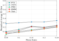
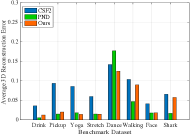
Refer to caption
(a)
Refer to caption
(b)
Figure 7: (a) 3D reconstruction error comparison over noisy trajectories. (b) Comparison of our method performance with other competing methods with missing data in the measurement matrix. Note: BMM was not formulated for missing data case, therefore, its results are not present in the above figures.

5 Conclusion

With weighted nuclear norm minimization of the shape matrix and an analytic solution to the rotation matrix based on the smoothness of the camera motion [27], we witnessed that the prior-free idea performs almost as good as the best available algorithm’s. Without exploiting the “prior-free” idea [9] fully based on the well-known assumptions of smooth deformation of the non-rigid object and its low-rank shape, it may perform badly, which might be the reason that researchers have had poor results using it, even for the non-rigid objects that span a single linear subspace. Our work revealed the possibility of making “prior-free” [9] practically more accurate under the different conditions of measurement matrix with elementary modifications, and also conjecture some open problems. The accuracy of our algorithm on the benchmark datasets empirically validates that the “prior-free” theory is still a very powerful way to solve NRSfM and therefore, the proposition before the NRSfM researchers to consider is, it’s not the failure of the concept behind the prior-free idea for its inferior performance but, it’s possibly due to our inability to correctly cater, and cleverly exploit the arc of information and perspectives provided by it to solve NRSfM.

Acknowlegment: The author research work is supported by Google and ETH Zürich Foundation project number 2019-HE-323 (2).

References

  • [1] I. Akhter, Y. Sheikh, S. Khan, and T. Kanade. Nonrigid structure from motion in trajectory space. In Advances in neural information processing systems, pages 41–48, 2009.
  • [2] I. Akhter, Y. Sheikh, S. Khan, and T. Kanade. Trajectory space: A dual representation for nonrigid structure from motion. IEEE Transactions on Pattern Analysis and Machine Intelligence, 33(7):1442–1456, 2011.
  • [3] S. Boyd, N. Parikh, E. Chu, B. Peleato, and J. Eckstein. Distributed optimization and statistical learning via the alternating direction method of multipliers. Foundations and Trends® in Machine Learning, 3(1):1–122, 2011.
  • [4] M. Brand. A direct method for 3d factorization of nonrigid motion observed in 2d. In 2005 IEEE Computer Society Conference on Computer Vision and Pattern Recognition (CVPR’05), volume 2, pages 122–128. IEEE, 2005.
  • [5] C. Bregler, A. Hertzmann, and H. Biermann. Recovering non-rigid 3d shape from image streams. In IEEE Conference on Computer Vision and Pattern Recognition, volume 2, pages 690–696. IEEE, 2000.
  • [6] R. Cabral, F. De la Torre, J. P. Costeira, and A. Bernardino. Unifying nuclear norm and bilinear factorization approaches for low-rank matrix decomposition. In Proceedings of the IEEE International Conference on Computer Vision, pages 2488–2495, 2013.
  • [7] J.-F. Cai, E. J. Candès, and Z. Shen. A singular value thresholding algorithm for matrix completion. SIAM Journal on Optimization, 20(4):1956–1982, 2010.
  • [8] Y. Dai, H. Li, and M. He. A simple prior-free method for non-rigid structure-from-motion factorization. In Computer Vision and Pattern Recognition (CVPR), 2012 IEEE Conference on, pages 2018–2025. IEEE, 2012.
  • [9] Y. Dai, H. Li, and M. He. A simple prior-free method for non-rigid structure-from-motion factorization. International Journal of Computer Vision, 107(2):101–122, 2014.
  • [10] P. F. Gotardo and A. M. Martinez. Kernel non-rigid structure from motion. In IEEE International Conference on Computer Vision, pages 802–809. IEEE, 2011.
  • [11] P. F. Gotardo and A. M. Martinez. Non-rigid structure from motion with complementary rank-3 spaces. In Computer Vision and Pattern Recognition (CVPR), 2011 IEEE Conference on, pages 3065–3072. IEEE, 2011.
  • [12] S. Gu, L. Zhang, W. Zuo, and X. Feng. Weighted nuclear norm minimization with application to image denoising. In Proceedings of the IEEE Conference on Computer Vision and Pattern Recognition, pages 2862–2869, 2014.
  • [13] R. Hartley, J. Trumpf, Y. Dai, and H. Li. Rotation averaging. International journal of computer vision, 103(3):267–305, 2013.
  • [14] S. H. N. Jensen, A. Del Bue, M. E. B. Doest, and H. Aanæs. A benchmark and evaluation of non-rigid structure from motion. arXiv preprint arXiv:1801.08388, 2018.
  • [15] S. Kumar. Jumping manifolds: Geometry aware dense non-rigid structure from motion. In IEEE, CVPR, pages 5346–5355, 2019.
  • [16] S. Kumar, A. Cherian, Y. Dai, and H. Li. Scalable dense non-rigid structure-from-motion: A grassmannian perspective. In IEEE, CVPR, pages 254–263, 2018.
  • [17] S. Kumar, Y. Dai, and H. Li. Multi-body non-rigid structure-from-motion. In 3D Vision (3DV), 2016 Fourth International Conference on, pages 148–156. IEEE, 2016.
  • [18] S. Kumar, Y. Dai, and H. Li. Monocular dense 3d reconstruction of a complex dynamic scene from two perspective frames. In IEEE, ICCV, pages 4649–4657, Oct 2017.
  • [19] S. Kumar, Y. Dai, and H. Li. Spatio-temporal union of subspaces for multi-body non-rigid structure-from-motion. Pattern Recognition, 71:428–443, May 2017.
  • [20] S. Kumar, Y. Dai, and H. Li. Superpixel soup: Monocular dense 3d reconstruction of a complex dynamic scene. IEEE Transactions on Pattern Analysis and Machine Intelligence (T-PAMI), 2019.
  • [21] V. Larsson and C. Olsson. Compact matrix factorization with dependent subspaces. In Proceedings of the IEEE Conference on Computer Vision and Pattern Recognition, pages 280–289, 2017.
  • [22] M. Lee, J. Cho, C.-H. Choi, and S. Oh. Procrustean normal distribution for non-rigid structure from motion. In IEEE Conference on Computer Vision and Pattern Recognition, pages 1280–1287, 2013.
  • [23] M. Lee, J. Cho, and S. Oh. Consensus of non-rigid reconstructions. In IEEE Conference on Computer Vision and Pattern Recognition, pages 4670–4678, 2016.
  • [24] G. Liu, Z. Lin, S. Yan, J. Sun, Y. Yu, and Y. Ma. Robust recovery of subspace structures by low-rank representation. IEEE Transactions on Pattern Analysis and Machine Intelligence, 35(1):171–184, 2013.
  • [25] C. Lu, J. Tang, S. Yan, and Z. Lin. Nonconvex nonsmooth low-rank minimization via iteratively reweighted nuclear norm. arXiv preprint arXiv:1510.06895, 2015.
  • [26] S. Ma, D. Goldfarb, and L. Chen. Fixed point and bregman iterative methods for matrix rank minimization. Mathematical Programming, 128(1-2):321–353, 2011.
  • [27] V. Rabaud and S. Belongie. Re-thinking non-rigid structure from motion. In IEEE Conference on Computer Vision and Pattern Recognition, pages 1–8. IEEE, 2008.
  • [28] N. Srebro and T. Jaakkola. Weighted low-rank approximations. In Proceedings of the 20th International Conference on Machine Learning (ICML-03), pages 720–727, 2003.
  • [29] J. Taylor, A. D. Jepson, and K. N. Kutulakos. Non-rigid structure from locally-rigid motion. In IEEE Conference on Computer Vision and Pattern Recognition, pages 2761–2768. IEEE, 2010.
  • [30] C. Tomasi and T. Kanade. Shape and motion from image streams under orthography: a factorization method. International Journal of Computer Vision, 9(2):137–154, 1992.
  • [31] L. Torresani, A. Hertzmann, and C. Bregler. Nonrigid structure-from-motion: Estimating shape and motion with hierarchical priors. IEEE transactions on pattern analysis and machine intelligence, 30(5):878–892, 2008.
  • [32] J. Valmadre, S. Sridharan, S. Denman, C. Fookes, and S. Lucey. Closed-form solutions for low-rank non-rigid reconstruction. In Digital Image Computing: Techniques and Applications (DICTA), 2015 International Conference on, pages 1–6. IEEE, 2015.
  • [33] J. Xiao, J.-x. Chai, and T. Kanade. A closed-form solution to non-rigid shape and motion recovery. In European conference on computer vision, pages 573–587. Springer, 2004.
  • [34] Z. Zha, X. Zhang, Y. Wu, Q. Wang, Y. Bai, and L. Tang. Analyzing the weighted nuclear norm minimization and nuclear norm minimization based on group sparse representation. arXiv preprint arXiv:1702.04463, 2017.
  • [35] D. Zhang, Y. Hu, J. Ye, X. Li, and X. He. Matrix completion by truncated nuclear norm regularization. In Computer Vision and Pattern Recognition (CVPR), 2012 IEEE Conference on, pages 2192–2199. IEEE, 2012.
  • [36] Y. Zhu, D. Huang, F. De La Torre, and S. Lucey. Complex non-rigid motion 3d reconstruction by union of subspaces. In IEEE Conference on Computer Vision and Pattern Recognition, pages 1542–1549, 2014.