High Flux Passive Imaging with Single-Photon Sensors

Abstract

Single-photon avalanche diodes (SPADs) are an emerging technology with a unique capability of capturing individual photons with high timing precision. SPADs are being used in several active imaging systems (e.g., fluorescence lifetime microscopy and LiDAR), albeit mostly limited to low photon flux settings. We propose passive free-running SPAD (PF-SPAD) imaging, an imaging modality that uses SPADs for capturing 2D intensity images with unprecedented dynamic range under ambient lighting, without any active light source. Our key observation is that the precise inter-photon timing measured by a SPAD can be used for estimating scene brightness under ambient lighting conditions, even for very bright scenes. We develop a theoretical model for PF-SPAD imaging, and derive a scene brightness estimator based on the average time of darkness between successive photons detected by a PF-SPAD pixel. Our key insight is that due to the stochastic nature of photon arrivals, this estimator does not suffer from a hard saturation limit. Coupled with high sensitivity at low flux, this enables a PF-SPAD pixel to measure a wide range of scene brightnesses, from very low to very high, thereby achieving extreme dynamic range. We demonstrate an improvement of over 2 orders of magnitude over conventional sensors by imaging scenes spanning a dynamic range of $10^{6}:1$.

1 Introduction

Figure 1: Conventional vs. PF-SPAD imaging. The top row shows photon detection timelines at low and high flux levels for the two types of sensor pixels. The middle row shows sensor response curves as a function of incident photon flux for a fixed exposure time. At high flux, a conventional sensor pixel saturates when the full well capacity is reached. A PF-SPAD pixel has a non-linear response curve with an asymptotic saturation limit and can operate even at extremely high flux levels. The bottom row shows simulated single-capture images of an HDR scene with a fixed exposure time of $5\text{\,}\mathrm{ms}$ for both types of sensors. The conventional sensor has a full well capacity of 33,400. The SPAD has a dead time of $149.7\text{\,}\mathrm{ns}$ which corresponds to an asymptotic saturation limit equal to 33,400. The hypothetical PF-SPAD array can simultaneously capture dark and bright regions of the scene in a single exposure time. The PF-SPAD image is for conceptual illustration only; megapixel PF-SPAD arrays are currently not available.

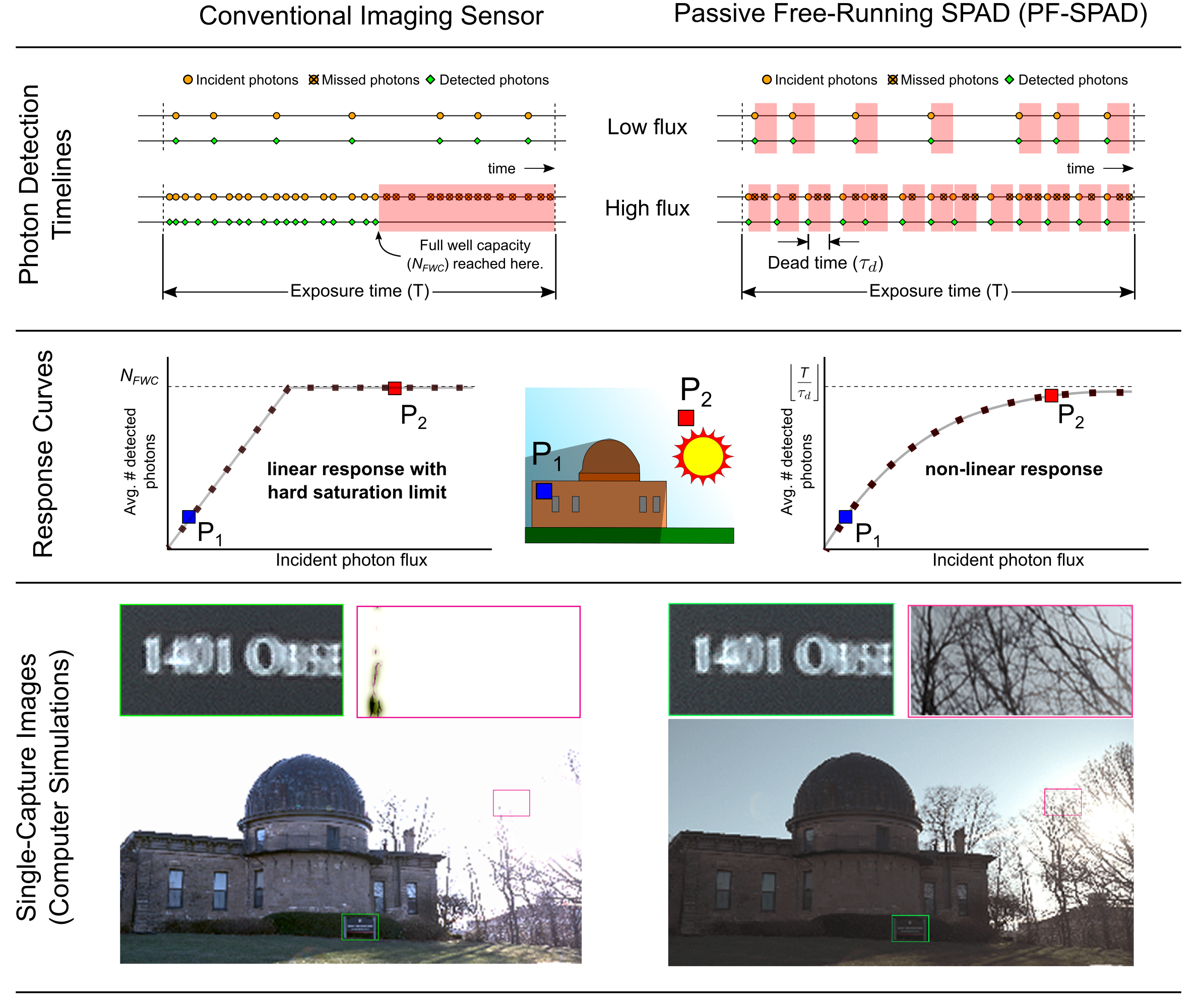
Single-photon avalanche diodes (SPADs) can count individual photons and capture their temporal arrival statistics with very high precision [1]. Due to this capability, SPADs are widely used in low light scenarios [2, 3, 4], LiDAR [5, 6] and non-line of sight imaging [7, 8, 9]. In these applications, SPADs are used in synchronization with an active light source (e.g., a pulsed laser). In this paper, we propose passive free-running SPAD (PF-SPAD) imaging, where SPADs are used in a free-running mode, with the goal of capturing 2D intensity images of scenes under passive lighting, without an actively controlled light source. Although SPADs have so far been limited to low flux settings, using the timing statistics of photon arrivals, PF-SPAD imaging can successfully capture much higher flux levels than previously thought possible.

We build a detailed theoretical model and derive a scene brightness estimator for PF-SPAD imaging that, unlike a conventional sensor pixel, does not suffer from full well capacity limits [10] and can measure high incident flux. Therefore, a PF-SPAD remains sensitive to incident light throughout the exposure time, even under very strong incident flux. This enables imaging scenes with large brightness variations, from extreme dark to very bright. Imagine an autonomous car driving out of a dark tunnel on a bright sunny day, or a robot inspecting critical machine parts made of metal with strong specular reflections. These scenarios require handling large illumination changes, that are often beyond the capabilities of conventional sensors.

Intriguing Characteristics of PF-SPAD Imaging: Unlike conventional sensor pixels that have a linear input-output response (except past saturation), a PF-SPAD pixel has a non-linear response curve with an asymptotic saturation limit as illustrated in Figure 1. After each photon detection event, the SPAD enters a fixed dead time interval where it cannot detect additional photons. The non-linear response is a consequence of the PF-SPAD adaptively missing a fraction of the incident photons as the incident flux increases (see Figure 1 top-right). Theoretically, a PF-SPAD sensor does not saturate even at extremely high brightness values. Instead, it reaches a soft saturation limit beyond which it still stays sensitive, albeit with a lower signal-to-noise ratio (SNR). This soft saturation point is reached considerably past the saturation limits of conventional sensors, thus, enabling PF-SPADs to reliably measure high flux values.

Various noise sources in PF-SPAD imaging also exhibit counter-intuitive behavior. For example, while in conventional imaging, photon noise increases monotonically (as square-root) with the incident flux, in PF-SPAD imaging, the photon noise first increases with incident flux, and then decreases after reaching a maximum value, until eventually, it becomes even lower than the quantization noise. Quantization noise dominates at very high flux levels. In contrast, for conventional sensors, quantization noise affects SNR only at very low flux; and when operating in realistic flux levels, photon noise dominates other sources of noise.

Extreme Dynamic Range Imaging with PF-SPADs: Due to their ability to measure high flux levels, combined with single-photon sensitivity, PF-SPADs can simultaneously capture a large range of brightness values in a single exposure, making them well suited as high dynamic range (HDR) imaging sensors. We provide theoretical justification for the HDR capability of PF-SPAD imaging by modeling its photon detection statistics. We build a hardware prototype and demonstrate single-exposure imaging of scenes with an extreme dynamic range of $10^{6}\!\!:\!\!1$, over 2 orders of magnitude higher than conventional sensors. We envision that the proposed approach and analysis will expand the applicability of SPADs as general-purpose, all-lighting-condition, passive imaging sensors, not limited to specialized applications involving low flux conditions or active illumination, and play a key role in applications that witness extreme variations in flux levels, including astronomy, microscopy, photography, and computer vision systems.

Scope and Limitations: The goal of this paper is to present the concept of adaptive temporal binning for passive flux sensing and related theoretical analysis using a single-pixel PF-SPAD implementation. Current SPAD technology is still in a nascent stage, not mature enough to replace conventional CCD and CMOS image sensors. Megapixel PF-SPAD arrays have not been realized yet. Various technical design challenges that must be resolved to enable high resolution PF-SPAD arrays are beyond the scope of this paper.

2 Related Work

HDR Imaging using Conventional Sensors: The key idea behind HDR imaging with digital CMOS or CCD sensors is similar to combination printing [11] — capture more light from darker parts of the scene to mitigate sensor noise and less light from brighter parts of the scene to avoid saturation. A widely used computational method called exposure bracketing [12, 13] captures multiple images of the scene using different exposure times and blends the pixel values to generate an HDR image.Exposure bracketing algorithms can be adapted to the PF-SPAD image formation model to further increase their dynamic range.

Hardware Modifications to Conventional Sensors: Spatially varying exposure technique modulates the amount of light reaching the sensor pixels using fixed [14] or adaptive [15] light absorbing neutral density filters. Another method [16] involves the use of beam-splitters to relay the scene onto multiple imaging sensors with different exposure settings. In contrast, our method can provide improved dynamic range without having to trade off spatial resolution.

Sensors with Non-Linear Response: Logarithmic image sensors [17] use additional hardware in each pixel that applies logarithmic non-linearity to obtain dynamic range compression. Quanta image sensors (QIS) obtain logarithmic dynamic range compression by exploiting fine-grained (sub-diffraction-limit) spatial statistics, through spatial oversampling [18, 19, 20]. We take a different approach of treating a SPAD as an adaptive temporal binary sensor which subdivides the total exposure time into random non-equispaced time bins at least as long as the dead time of the SPAD. Experimental results in recent work [21] have shown the potential of this method for improved dynamic range over the QIS approach. Here we provide a comprehensive theoretical justification by deriving the SNR from first principles and also show simulated and experimental imaging results demonstrating dynamic range improvements of over two orders of magnitude.

3 Passive Imaging with a Free-Running SPAD

In this section we present an image formation model for a PF-SPAD and derive a photon flux estimator that relies on inter-photon detection times and photon counts. This provides formal justification for the notion of adaptive photon rejection and the asymptotic response curve of a PF-SPAD.

Each PF-SPAD pixel passively measures the photon flux from a scene point by detecting incident photons over a fixed exposure time. The time intervals between consecutive incident photons vary randomly according to a Poisson process [22]. If the difference in the arrival times of two consecutive photons is less than the SPAD dead time, the later photon is not detected. The free-running operating mode means that the PF-SPAD pixel is ready to capture the next available photon as soon as the dead time interval from the previous photon detection event elapses. In this free-running, passive-capture mode the PF-SPAD pixel acts as a temporal binary sensor that divides the total exposure time into random, non-uniformly spaced time intervals, each at least as long as the dead time. As shown in Figure 1, the PF-SPAD pixel detects at most one photon within each interval; additional incident photons during the dead time interval are not detected. The same figure also shows that as the average number of photons incident on a SPAD increases, the fraction of the number of detected photons decreases.

PF-SPAD Image Formation Model: Suppose the PF-SPAD pixel is exposed to a constant photon flux of $\Phi$ photons per unit time over a fixed exposure time $T$. Let $N_{T}$ denote the total number of photons detected in time $T$, and $\{X_{1},X_{2},\ldots,X_{N_{T}-1}\}$ denote the inter-detection time intervals. We define the average time of darkness as $\bar{X}=\frac{1}{N_{T}-1}\sum_{i=1}^{N_{T}-1}{X_{i}}$. Intuitively, a larger incident flux should correspond to a lower average time of darkness, and vice versa. Based on this intuition, we derive the following estimator of the incident flux as a function of $\bar{X}$ (see Supplementary Note 1 for derivation):

$$\hat{\Phi}=\frac{1}{q\left(\bar{X}-\tau_{d}\right)},$$ (1)

where $\hat{\Phi}$ denotes the estimated photon flux, $0<q<1$ is the photon detection probability of the SPAD pixel, and $\tau_{d}$ is the dead time. Note that since $X_{i}\geq\tau_{d}\,\,\forall\,i$, the estimator in Equation (1) is positive and finite. In a practical implementation, it is often more efficient to use fast counting circuits that only provide a count of the total number of SPAD detection events in the exposure time interval, instead of storing timestamps for individual detection events. In this case, the average time of darkness can be approximated as $\bar{X}\approx T/N_{T}$. The flux estimator that uses only photon counts is given by:

$$\underbrace{\boxed{\hat{\Phi}=\,\frac{N_{T}}{q\left(T-N_{T}\,\tau_{d}\right)}}}_{\text{{PF-SPAD Flux Estimator}}}.$$ (2)

Interpreting the PF-SPAD Flux Estimator: The photon flux estimator in Equation (2) is a function of the number of photons detected by a dead time-limited SPAD pixel and is valid at all incident flux levels. The image formation procedure applies this inverse non-linear mapping to the photon counts from each PF-SPAD pixel to recover flux values, even for bright parts of the scene. The relationship between the estimated flux, $\hat{\Phi}$, and the number of photons detected, $N_{T}$, is non-linear, and is similar to the well-known non-paralyzable detector model used to describe certain radioactive particle detectors [23, 24].

To obtain further insight into the non-linear behaviour of a SPAD pixel in the free-running mode, it is instructive to analyze the average number of detected photons as a function of $\Phi$ for a fixed $T$. Using the theory of renewal processes [24] we can show that:

$$\mathbf{E}[N_{T}]=\frac{q\Phi T}{1+q\Phi\tau_{d}}\,.$$ (3)

This non-linear SPAD response curve is shown in Figure 1. The non-linear behavior is a consequence of the ability of a SPAD to perform adaptive photon rejection during the exposure time. The shape of the response curve is similar to a gamma-correction or tone-mapping curve used for displaying an HDR image. As a result, the SPAD response curve provides dynamic range compression, gratis, with no additional hardware modifications. The key observation about Equation (3) is that it has an asymptotic saturation limit given by $\lim_{\Phi\rightarrow\infty}\mathbf{E}[N_{T}]=T/\tau_{d}$. Therefore, in theory, the photon counts never saturate because this asymptotic limit can only be achieved with an infinitely bright light source. In practice, as we discuss in the following sections, due to the inherent quantized nature of photon counts, the estimator in Equation (2) suffers from a soft saturation phenomenon at high flux levels and limits the SNR.

4 Peculiar Noise Characteristics of PF-SPADs

In this section, we list various noise sources that affect a PF-SPAD pixel, derive mathematical expressions for the bias and variance they introduce in the total photon counts, and provide intuition on their surprising, counter-intuitive characteristics as compared to a conventional pixel. Ultimately, the flux estimation performance limits will be determined by the cumulative effect of these sources of noise as a function of the incident photon flux.

Figure 2: Effect of various sources of noise on variance of PF-SPAD photon counts. For a PF-SPAD pixel, the variance in photon counts due to quantization remains constant at all flux levels. The variance due to shot noise first increases and then decreases with increasing incident flux. At the soft saturation point, quantization exceeds shot noise variance. For a conventional pixel, quantization noise remains small and constant until the full well capacity is reached, where it jumps to infinity. Shot noise variance increases monotonically with incident flux.

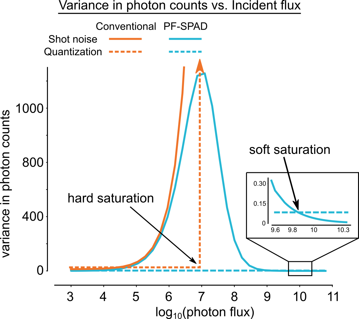
Shot Noise: For a conventional image sensor, due to Poisson distribution of photon arrivals, the variance of shot noise is proportional to the incident photon flux [22], as shown in Figure 2. A PF-SPAD, however, adaptively rejects a fraction of the incident photons during the dead time. Therefore, although the incident photons follow Poisson statistics, the photon counts (number of detected photons) do not. We define shot noise for PF-SPADs as the variance in the detected number of photon counts. This is approximately given by (see Supplementary Note 2):

$$\mathrm{Var}[N_{T}]=\frac{q\,\Phi\,T}{(1+q\,\Phi\,\tau_{d})^{3}}.$$ (4)

As shown in Figure 2, the variance first increases as a function of incident flux, reaches a maximum and then decreases at very high flux levels. This peculiar behavior can be understood intuitively from the PF-SPAD photon detection timelines in Figure 1 and observing how the dead time intervals are spread within the exposure time. At low flux, when $\Phi\ll 1/\tau_{d}$, the dead time windows, on average, have large intervening time gaps. So the detected photon count statistics behave approximately like a conventional image sensor with Poisson statistics: $\mathrm{Var}[N_{T}]\approx q\Phi T$. This explains the monotonically increasing trend in variance at low flux. However, for large incident flux $\Phi\gg 1/\tau_{d}$ the time of darkness between consecutive dead time windows becomes sufficiently small that the PF-SPAD detects a photon soon after the preceding dead time interval expires. This causes a decrease in randomness which manifests as a monotonically decreasing photon count variance. In theory, as $\Phi\rightarrow\infty$ the process becomes deterministic with zero variance: the PF-SPAD detects exactly one photon per dead time window.

Quantization Noise and Saturation: For a PF-SPAD, since the photon counts are always integer valued, the source of quantization noise is inherent in the measurement process. As a first order approximation, this can be modeled as being uniformly distributed in the interval $[0,1]$ which has a variance of $\nicefrac{{1}}{{12}}$ for all incident flux levels. A surprising consequence of the monotonically decreasing behavior of PF-SPAD shot noise is that at sufficiently high photon flux, quantization noise exceeds shot noise and becomes the dominant source of noise. This shown in Figure 2 (zoomed inset). We refer to this phenomenon as soft saturation, and discuss this in more detail in the next section.

In contrast, for a conventional imaging sensor, quantization noise is often ignored at high incident flux levels because state of the art CMOS and CCD sensors have analog-to-digital conversion (ADC) with sufficient bit depths. However, these sensors suffer from full well capacity limits beyond which they can no longer detect incident photons. As shown in Figure 2, we incorporate this hard saturation limit into quantization noise by allowing the quantization variance to jump to infinity when the full well capacity is reached.

Dark Count and Afterpulsing Noise: Dark counts are spurious counts caused by thermally generated electrons and can be modeled as a Poisson process with rate $\Phi_{\mathrm{dark}}$, independent of the true photon arrivals. Afterpulsing noise refers to spurious counts caused due to charged carriers that remain trapped in the SPAD from preceding photon detections. In most modern SPAD detectors dark counts and afterpulsing effects are usually negligible and can be ignored.

Effect of Noise on Scene Brightness Estimation: Since the output of a conventional sensor pixel is linear in the incident brightness, the variance in estimated brightness is simply equal (up to a constant scaling factor) to the noise variance. This is not the case for a PF-SPAD pixel due to its non-linear response curve — the variance in photon counts due to different sources of noise must be converted to a variance in brightness estimates, by accounting for the non-linear dependence of $\hat{\Phi}$ on $N_{T}$ in Equation (2). This raises a natural question: Given the various noise sources that affect the photon counts obtained from a PF-SPAD pixel, how reliable is the estimated scene brightness?

5 Extreme Dynamic Range of PF-SPADs

The various sources of noise in a PF-SPAD pixel described in the previous section cause the estimated photon flux $\hat{\Phi}$ to deviate from the true value $\Phi$. In this section we derive mathematical expressions for the bias and variance introduced by these different sources of noise in the PF-SPAD flux estimate. The cumulative effect of these errors is captured in the root-mean-squared error (RMSE) metric:

$$\mathsf{RMSE}(\hat{\Phi})=\sqrt{\mathbf{E}[(\hat{\Phi}-\Phi)^{2}]},$$

where the expectation operation averages over all the sources of noise in the SPAD pixel. Using the bias-variance decomposition, the RMSE of the PF-SPAD flux estimator can be decomposed as a sum of flux estimation errors from the different sources of noise:

Figure 3: Signal-to-noise ratio of a PF-SPAD pixel. (a) A PF-SPAD pixel suffers from quantization noise, which results in flux estimation error that increases as a function of incident flux. Beyond a flux level denoted as “soft saturation,” quantization becomes the dominant noise source overtaking shot noise. In contrast, for conventional sensors, quantization and read noise remain constant while shot noise increases with incident flux. (b) Unlike a conventional sensor, a PF-SPAD sensor does not suffer from a hard saturation limit. A soft saturation response leads to a graceful drop in SNR at high photon flux, leading to a high dynamic range. (c) An experimental SNR plot obtained from a hardware prototype consisting of a $25\text{\,}\mathrm{\SIUnitSymbolMicro m}$ PF-SPAD pixel with a $149.7\pm$6\text{\,}\mathrm{ns}$$ dead time and $5\text{\,}\mathrm{ms}$ exposure time.

$$\mathsf{RMSE}(\hat{\Phi})\!=\!\sqrt{(\Phi_{\mathrm{dark}}\!+\!B_{\mathrm{ap}})^{2}+\!V_{\text{shot}}\!+\!V_{\mathrm{quantization}}}\,.$$ (5)

The variance in the estimated flux due to shot noise (Equation (4)) is given by:

$$V_{\mathrm{shot}}=\frac{\Phi(1+q\Phi\tau_{d})}{qT}.$$ (6)

The variance in estimated flux due to quantization is:

$$V_{\mathrm{quantization}}=\frac{(1+q\Phi\tau_{d})^{4}}{12q^{2}T^{2}}.$$ (7)

The dark count bias $\Phi_{\mathrm{dark}}$ depends on the operating temperature. Finally, the afterpulsing bias $B_{\mathrm{ap}}$ can be expressed in terms of the afterpulsing probability $p_{\mathrm{ap}}$:

$$B_{\mathrm{ap}}=p_{\mathrm{ap}}\,q\Phi\,(1+\Phi\tau_{d})e^{-q\Phi\tau_{d}}.$$ (8)

See Supplementary Note 2 and Supplementary Note 3 for detailed derivations of Equations (6–8).

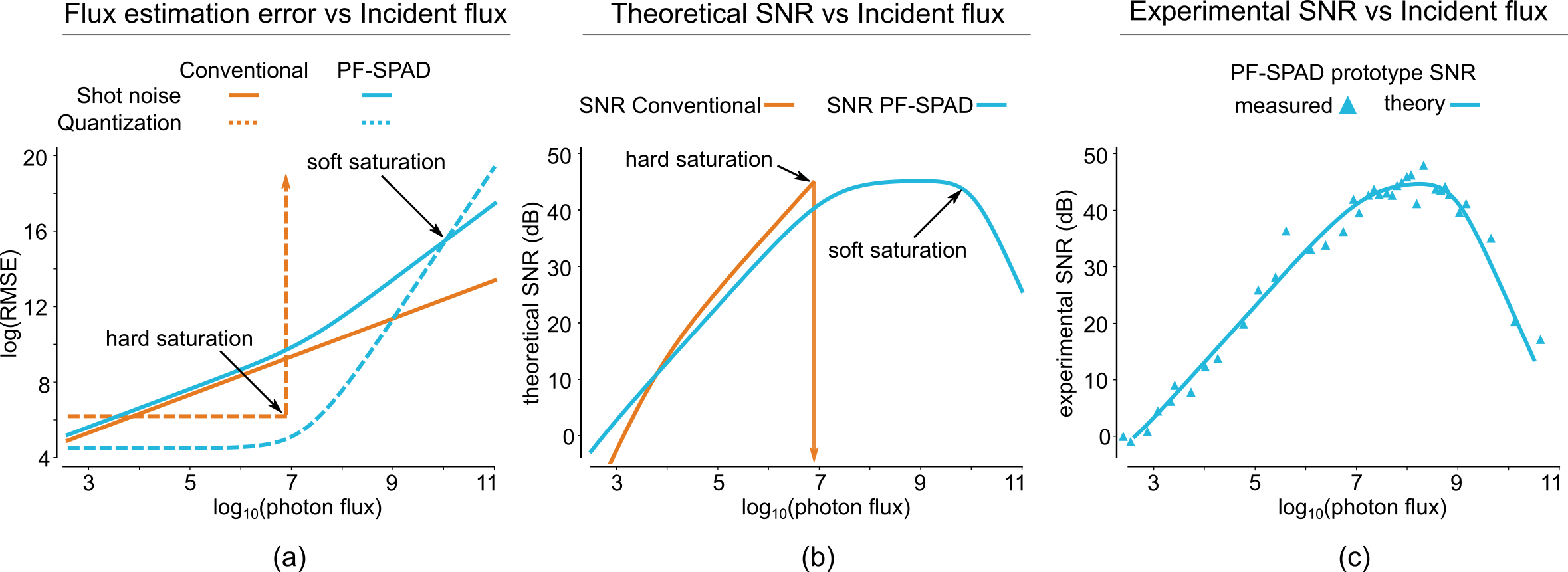
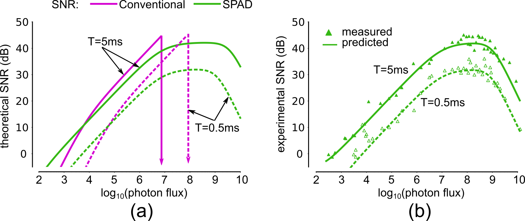
Figure 3(a) shows the flux estimation errors introduced by the various noise sources as a function of the incident flux levels for a conventional and a PF-SPAD pixel. The performance of the PF-SPAD flux estimator can be expressed in terms of its SNR, formally defined as the ratio of the true photon flux to the RMSE of the estimated flux [18]:

$$\mathsf{SNR}(\Phi)=20\log_{10}\left(\frac{\Phi}{\mathsf{RMSE}(\hat{\Phi})}\right).$$ (9)

By substituting the expressions for various noise sources from Equations (5-7) into Equation (9), we get an expression for the SNR of the SPAD-based flux estimator shown in Equation (10). Figure 3(b) shows the theoretical SNR as a function of incident flux for the PF-SPAD flux estimator, and a conventional sensor. A conventional sensor suffers from an abrupt drop in SNR due to hard saturation (see Supplementary Note 5). In contrast, the SNR achieved by a SPAD sensor degrades gracefully, even beyond the soft saturation point.

The Soft Saturation Phenomenon: It is particularly instructive to observe the behavior of quantization noise for the SPAD pixel. Although the quantization noise in the detected photon counts remains small and constant at all flux levels, the variance in the estimated flux due to quantization increases monotonically with incident flux. This is due to the non-linear nature of the estimator in Equation (2). At high incident flux levels, a single additional detected photon maps to a large range of estimated flux values, resulting in large errors in estimated flux. We call this phenomenon soft saturation. Beyond the soft saturation flux level, quantization dominates all other noise sources, including shot noise. The soft saturation limit, however, is reached at considerably higher flux levels as compared to the hard saturation limit of conventional sensors, thus, enabling PF-SPADs to reliably estimate very high flux levels.

$$\boxed{\mathsf{SNR}(\Phi)\!=\!-10\log_{10}\left[\left(\frac{\Phi_{\mathrm{dark}}}{\Phi}\!+\!q(1\!+\!\Phi\tau_{d})p_{\mathrm{ap}}e^{-q\Phi\tau_{d}}\right)^{2}\!+\!\frac{(1+q\Phi\tau_{d})}{q\Phi T}\!+\!\frac{(1+q\Phi\tau_{d})^{4}}{12q^{2}\Phi^{2}T^{2}}\right]}\,.$$ (10)

Effect of Varying Exposure Time: For conventional imaging sensors, increasing the exposure time causes the sensor pixel to saturate at a lower value of the incident flux level. This is equivalent to a horizontal translation of the conventional sensor’s SNR curve in Figure 3(b). This does not affect its dynamic range. However, for a PF-SPAD pixel, the asymptotic saturation limit increases linearly with the exposure time, hence increasing the SNR at all flux levels. This leads to a remarkable behavior of increasing the dynamic range of a PF-SPAD pixel with increasing exposure time. See Supplementary Note 6 and Supplementary Figure 2.

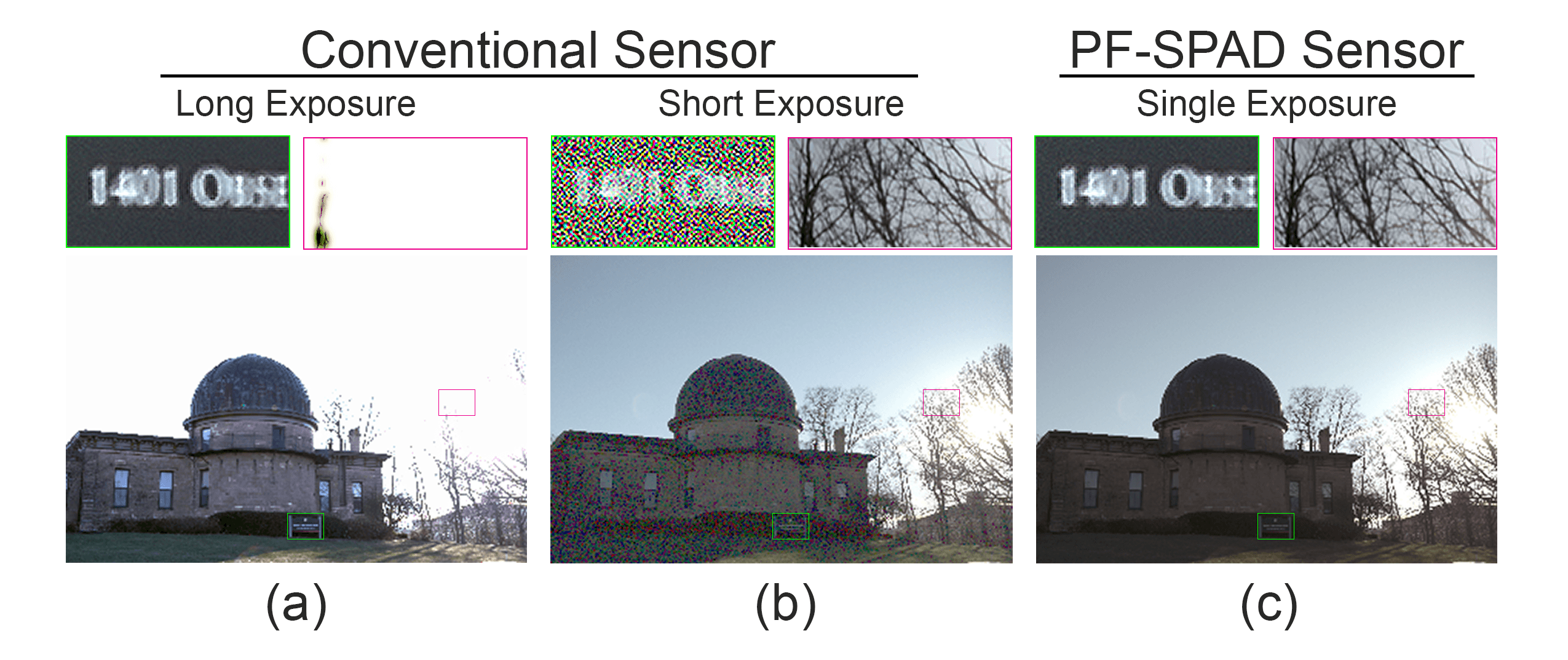
Simulated Megapixel PF-SPAD Imaging System: Figure 1 (bottom row) shows simulated images for a conventional megapixel image sensor array and a hypothetical megapixel PF-SPAD array. The ground truth photon flux image was obtained from an exposure bracketed HDR image captured using a Canon EOS Rebel T5 DSLR camera with 10 stops rescaled to cover a dynamic range of $10^{6}:1.$ An exposure time of $T=$5\text{\,}\mathrm{ms}$$ was used to simulate both images. For fair comparison, the SPAD dead time was set to $149.7\text{\,}\mathrm{ns}$, which corresponds to an asymptotic saturation limit of $\nicefrac{{T}}{{\tau_{d}}}=$34\,000$$, equal to the conventional sensor full well capacity. The quantum efficiencies of the conventional sensor and PF-SPAD were set to 90% and 40%. Observe that the PF-SPAD can simultaneously capture details in the dark regions of the scene (e.g. the text in the shadow) and bright regions in the sun-lit sky. The conventional sensor array exhibits saturation artifacts in the bright regions of the scene. (See Supplementary Note 7).

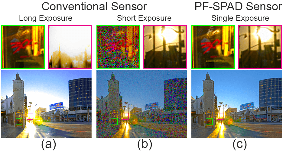
The human eye has a unique ability to adapt to a wide range of brightness levels ranging from a bright sunny day down to single photon levels [25, 26]. Conventional sensors cannot simultaneously reliably capture very dark and very bright regions in many natural scenes. In contrast, a PF-SPAD can simultaneously image dark and bright regions of the scene in a single exposure. Additional simulation results are shown in Supplementary Figures 7–9.

6 Experimental Results

SNR and Dynamic Range of a Single-Pixel PF-SPAD:

Figure 3(c) shows experimental SNR measurements using our prototype single-pixel SPAD sensor together with the SNR predicted by our theoretical model. Our hardware prototype has an additional $6\text{\,}\mathrm{ns}$ jitter introduced by the digital electronics that control the dead time window duration. This is not included in the SNR curve of Figure 3(b) but is accounted for in the theoretical SNR curve shown in Figure 3(c). See Supplementary Note 8 for details. We define dynamic range as the ratio of largest to smallest photon flux values that can be measured above a specified minimum SNR. Assuming a minimum acceptable SNR of 30 dB, the SPAD pixel achieves a dynamic range improvement of over 2 orders of magnitude compared to a conventional sensor.

Figure 4: Experimental single-pixel PF-SPAD imaging system. A free-running SPAD is mounted on two translation stages to raster-scan the image plane. There is no active light source—the PF-SPAD passively measures ambient light in the scene. Photon counts are captured using a single-photon counting module (not shown) operated without a synchronization signal.

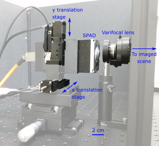
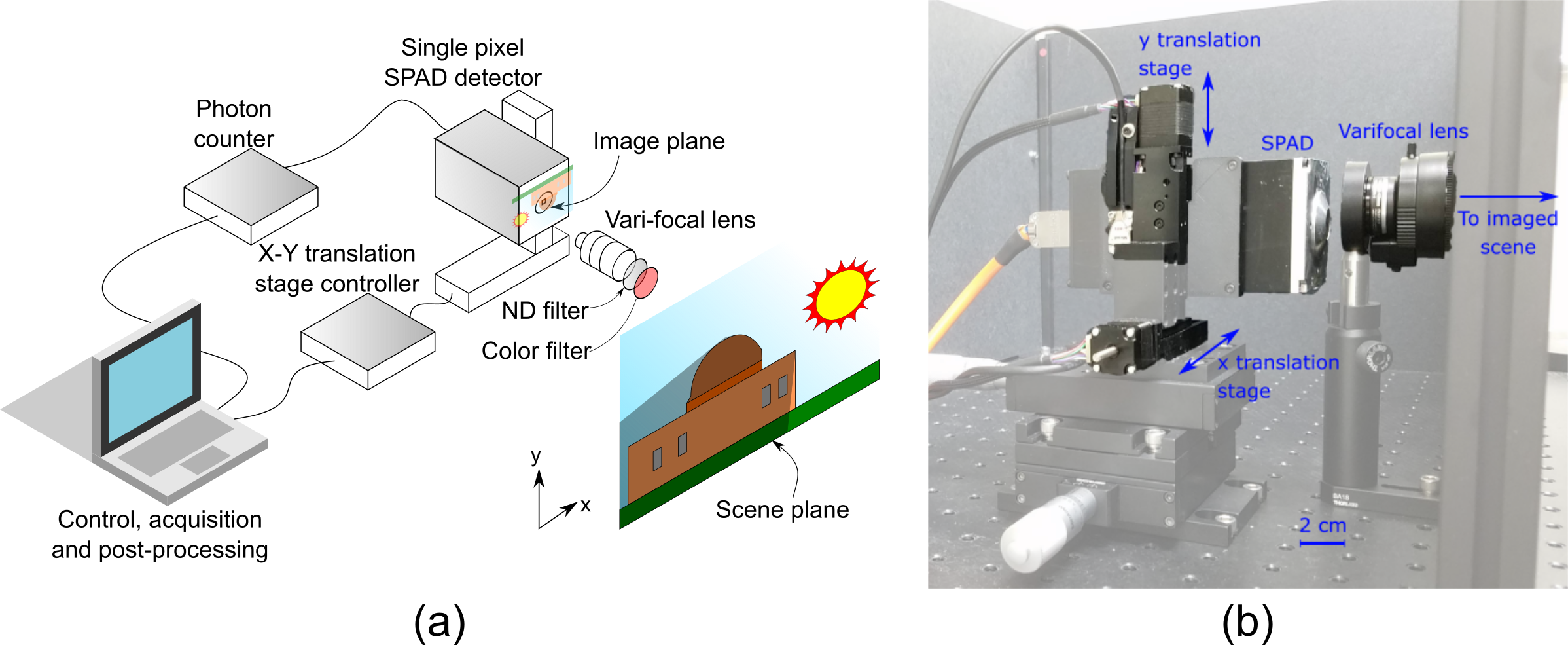
Point-Scanning Setup: The imaging setup shown in Figure 4 consists of a SPAD module mounted on a pair of micro-translation stages (VT-21L Micronix USA) to raster-scan the image plane of a variable focal length lens (Fujifilm DV3.4x3.8SA-1). Photon counts were recorded using a single-photon counting module (PicoQuant HydraHarp 400), with the SPAD in the free-running mode. A monochrome machine vision camera (FLIR GS3-U3-23S6M-C) was used for qualitative comparisons with the images acquired using the SPAD setup. The machine vision camera uses the same variable focal length lens with identical field of view as the scene imaged by the SPAD point-scanning setup. This ensures a comparable effective incident flux on a per-pixel basis for both the SPAD and the machine vision camera. The sensor pixel parameters are identical to those used in simulations. Images captured with the machine vision camera were downsampled to match the resolution of the raster-scanned PF-SPAD images.

Figure 5: Experimental comparison of the dynamic range of a CMOS camera and PF-SPAD imaging. The two imaged scenes have a wide range of brightness values (1,000,000:1), considerably beyond the dynamic range of conventional sensors. (a, d) Images captured using a 12-bit CMOS machine vision camera with a long exposure time of $5\text{\,}\mathrm{ms}$. Bright regions appear saturated. (b, e) Images of the same scenes with a short exposure time of $0.5\text{\,}\mathrm{ms}$. Darker regions appear grainy and severely underexposed, making it challenging to read the text on the signs and the numbers on the alarm clock. (c, f) PF-SPAD images of the same scenes captured using a single $5\text{\,}\mathrm{ms}$ exposure per pixel. Our hardware prototype captures the full range of brightness levels in the scenes in a single shot. The text is visible in both bright and dark regions of the scene, and details in regions of high flux, such as the filament of the bulb, can be recovered. For fair comparison, the main images were tone-mapped using the same tone-mapping algorithm.

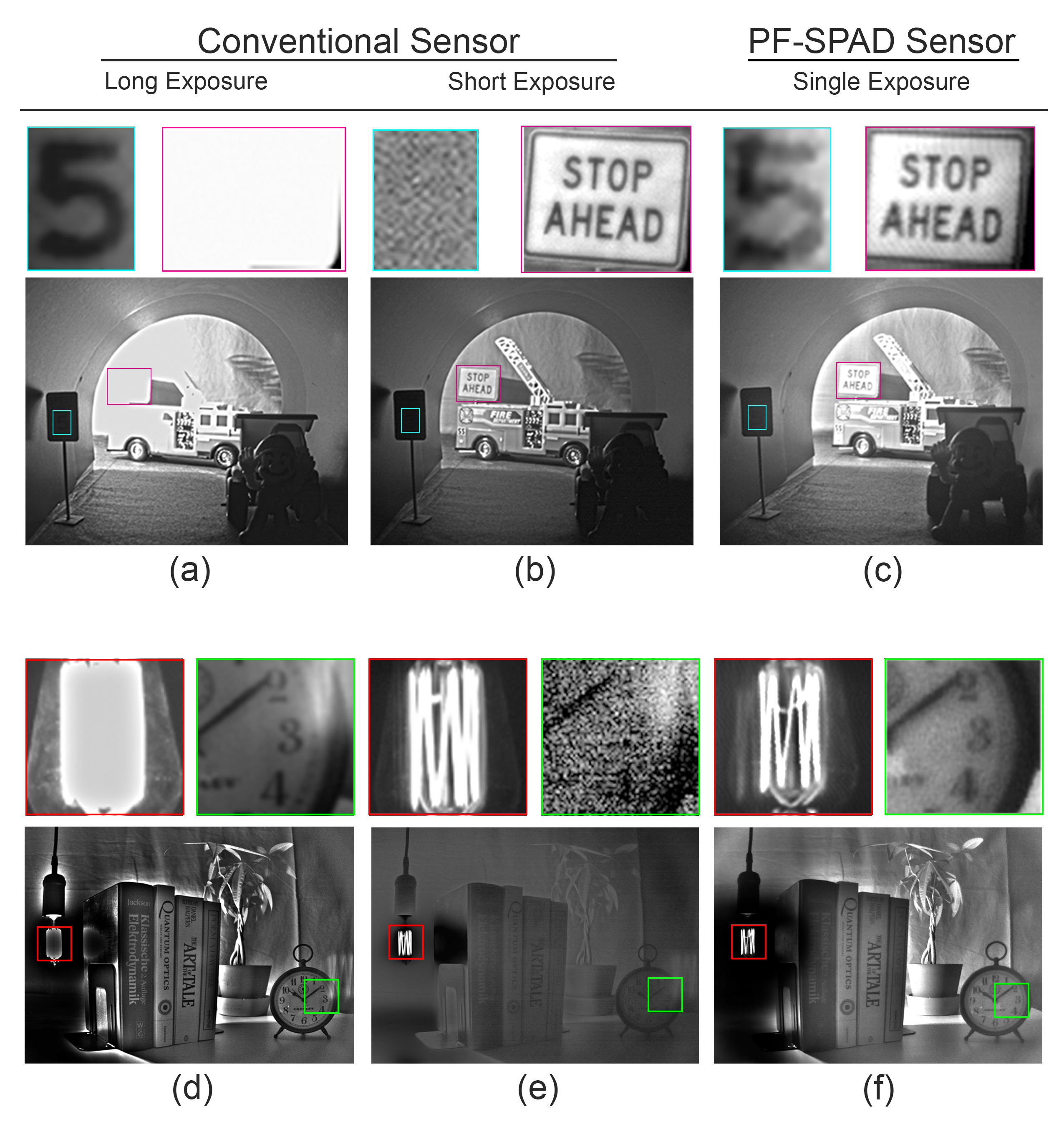
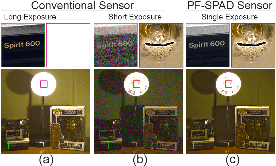
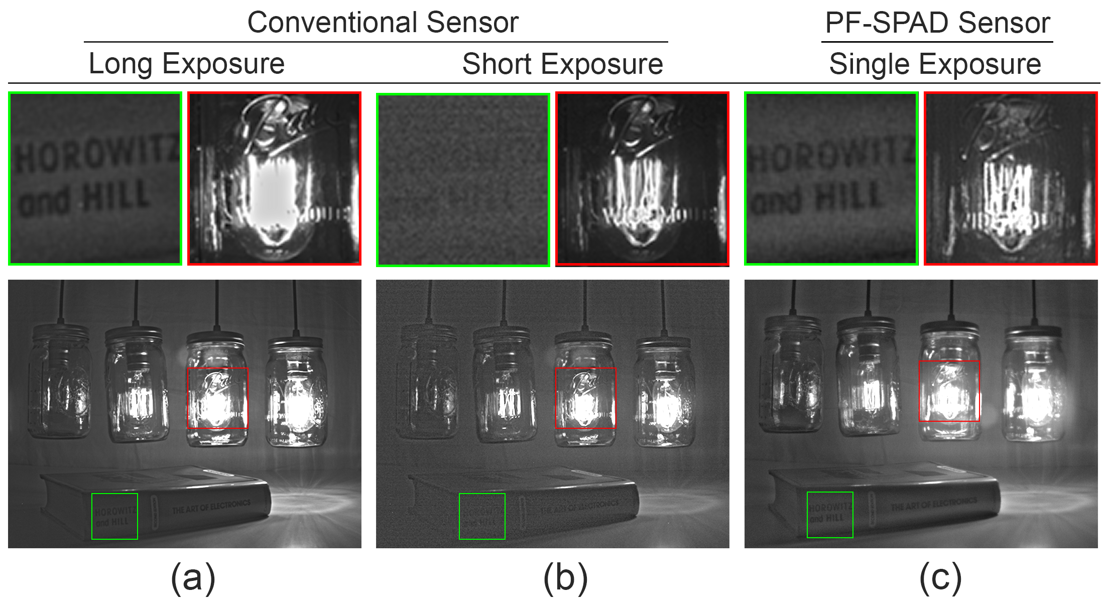
Extreme HDR: Results of single-shot HDR images from our raster-scanning PF-SPAD prototype are shown in Figure 5 and Supplementary Figure 10, for different scenes spanning a wide dynamic range ($\geq 10^{6}:1$) of brightness values. To reliably visualize the wide range of brightnesses in these scenes, three different tone-mapping algorithms were used to tone-map the main figures, the dark zoomed insets and the bright zoomed insets, respectively. The machine vision camera fails to capture bright text outside the tunnel (Fig. 5(a)) and dark text in the tunnel (Fig. 5(b)) in a single exposure interval. The PF-SPAD successfully captures the entire dynamic range (Fig. 5(c)). In Fig. 5(f), the PF-SPAD even captures the bright filament of an incandescent bulb simultaneously with dark text in the shadow. The halo artifacts in Figure 5(d–f) are due to a local adaptation-based non-invertible tone-map that was used to simultaneously visualize the bright filament and the dark text. This ability of the PF-SPAD flux estimator to capture a wide range of flux from very low to high in a single capture can have implications in many applications [27, 28, 29, 30]. that require extreme dynamic range.

7 Discussion

Quanta Image Sensor: An alternative realization [31] of a SPAD-based imaging sensor divides the total exposure time $T$ into uniformly spaced intervals of duration $\tau_{b}\geq\tau_{d}$. This “uniform-binning” method leads to a different image formation model which is known in literature as the oversampled binary image sensor [18] or quanta image sensor (QIS) [19, 20]. In Supplementary Note 9, we show that in theory, this uniform-binning implementation has a smaller dynamic range as compared to a PF-SPAD that allows the dead time windows to shift adaptively [21]. Note, however, that state of the art QIS technology provides much higher resolution and fill factor with high quantum efficiencies, and lower read noise than current SPAD arrays.

Limitations and Future Outlook: Our proof-of-concept imaging system uses a SPAD that is not optimized for operating in the free-running mode. The duration of the dead time window, which is a crucial parameter in our flux estimator, is not stable in current SPAD implementations (such as silicon photo-multipliers) as it is not crucial for active time-of-flight applications. Various research and engineering challenges must be met to realize a high resolution SPAD-based passive image sensor. State of the art SPAD pixel arrays that are commercially available today consist of thousands of pixels with row or column multiplexed readout capabilities and do not support fully parallel readout. Current SPAD arrays also have very low fill factors due to the need of integrating counting and storage electronics within each pixel [32, 33]. Our method and results make a case for developing high resolution fabrication and 3D stacking techniques that will enable high fill-factor SPAD arrays, which can be used as general purpose, passive sensors for applications requiring extreme dynamic range imaging.

Supplementary Note 1 Image Formation Model and Flux Estimator for a PF-SPAD Pixel

A PF-SPAD sensor pixel and a time-correlated photon counting module are used to obtain total photon counts over a fixed exposure time together with picosecond resolution measurements of the time elapsed between successive photon detection events. We will assume that the PF-SPAD pixel is exposed to a true photon flux of $\Phi$ photons/second for an exposure time of $T$ seconds and it records $N_{T}$ photons in exposure time interval $(0,T]$. For mathematical convenience, we assume that the exposure interval starts with a photon detection event at time $t=0$.

Photons arrive at the SPAD according to a Poisson process. Accounting for an imperfect photon detection efficiency of $0<q<1$, the time between consecutive incident photons follows an exponential distribution with rate $q\Phi.$ After each detection event, the SPAD enters a dead time window of duration $\tau_{d}$. Due to the memoryless property of Poisson processes [6], the time interval between the end of a dead time window and the next photon arrival is also exponentially distributed and has the same rate $q\Phi$ as the incident Poisson process. Let $X_{1}$ be the time of the first photon detection after $t=0$ and $X_{n}$ be the time between the $n-1^{st}$ and $n^{th}$ detection event for $n\geq 2$. Then the inter-detection time duration $X_{n}$ follows a shifted exponential distribution given by:

$$X_{n}\stackrel{{\scriptstyle iid}}{{\sim}}f_{X_{n}}(t)=\begin{cases}q\Phi e^{-q\Phi(t-\tau_{d})}&\mbox{for }t\geq\tau_{d}\\ 0&\mbox{otherwise.}\end{cases}$$ (S1)

This provides a probabilistic model of the photon inter-detection times. We now derive a flux estimator from a sequence of observed inter-detection times captured by a PF-SPAD pixel.

Estimating Flux from Inter-Detection Time Intervals

The log-likelihood function for the observed inter-detection times is given by

$$\log l(q\Phi;X_{1},\ldots,X_{N_{T}}) =\log\left(\prod_{n=1}^{N_{T}}q\Phi\,e^{-q\Phi(X_{n}-\tau_{d})}\right)$$

$$=-q\Phi\left(\sum_{n=1}^{N_{T}}X_{n}-\tau_{d}N_{T}\right)+N_{T}\log q\Phi$$

$$=-q\Phi\,N_{T}\,\left(\bar{X}-\tau_{d}\right)+N_{T}\log q\Phi$$ (S2)

where $\bar{X}:=\frac{1}{N_{T}}\sum_{n=1}^{N_{T}}X_{n}$ is the mean time between photon detection events. The maximum likelihood estimate $\hat{\Phi}$ of the true photon flux is computed by setting the derivative of Equation (S2) to zero:

$$\frac{N_{T}}{q\hat{\Phi}}-N_{T}(\bar{X}-\tau_{d})=0$$

which implies

$$\hat{\Phi}=\frac{1}{q}\frac{1}{\bar{X}-\tau_{d}}.$$ (S3)

Supplementary Note 2 Approximate Closed Form Formula for SNR of a PF-SPAD pixel

We first derive an approximate formula for the SNR of a PF-SPAD pixel using a continuous Gaussian distribution approximation for the number of counts $N_{T}$. The effective incident photon flux for a quantum efficiency of $0<q<1$ is equal to $q\Phi$ photons/second.

The random process describing the detections of this PF-SPAD pixel is not a Poisson process, but can be modeled as a renewal process [6] with a shifted exponential inter-arrival distribution which has a mean $\tau_{d}+\frac{1}{q\Phi}$ and variance $\frac{1}{q^{2}\Phi^{2}}$. Using the central limit theorem for renewal processes, $N_{T}$ is approximately Gaussian distributed with mean:

$$\mathbf{E}[N_{T}]=\frac{q\Phi T}{1+q\Phi\tau_{d}}$$

and variance:

$$\mathrm{Var}[N_{T}]=\frac{q\Phi T}{(1+q\Phi\tau_{d})^{3}}.$$

Quantization Noise: An additional source of variance arises due to quantization noise which we can treat as uniformly distributed between $0$ and $1$ with variance $1/12$. The c.d.f. of the estimated photon flux $\hat{\Phi}$ can be computed using the delta method [3]:

$$F_{\hat{\Phi}}(x) =\mathsf{Pr}(\hat{\Phi}\leq x)$$ (S4)

$$=\mathsf{Pr}\left(\frac{1}{q}\frac{N_{T}}{T-\tau_{d}N_{T}}\leq x\right)$$ (S5)

$$\approx\mathsf{Pr}\left(N_{T}\leq\frac{qxT}{1+qx\tau_{d}}\right)$$ (S6)

$$=\frac{1}{2}\left(1+\mathrm{erf}\left(\frac{\frac{qxT}{1+qx\tau_{d}}-\frac{q\Phi T}{1+q\Phi\tau_{d}}}{\sqrt{2}\sqrt{\frac{q\Phi T}{(1+q\Phi\tau_{d})^{3}}+\frac{1}{12}}}\right)\right)$$ (S7)

$$\approx\frac{1}{2}\left(1+\mathrm{erf}\left(\frac{x-\Phi}{\sqrt{2}\sqrt{\frac{\Phi(1+q\Phi\tau_{d})}{qT}+\frac{(1+q\Phi\tau_{d})^{4}}{12q^{2}T^{2}}}}\right)\right)$$ (S8)

where Equation (S6) follows from the fact that in practice the denominator is always non-negative since $N_{T}\leq\lfloor T/\tau_{d}\rfloor$, Equation (S7) follows from the formula for the Gaussian c.d.f. of $N_{T}$ with $\mathrm{erf}$ denoting the error function [1], and Equation (S8) is follows from a first order Taylor series approximation. This result shows that $\hat{\Phi}$ is approximately normally distributed with mean equal to the true photon flux and variance given by the denominator in Equation (S8).

Dark Count and Afterpulsing Bias: In addition to quantization and shot noise that introduce variance in the estimated photon flux, PF-SPADs also suffer from dark counts and afterpulsing noise that introduce a bias in the estimated flux. The dark count rate $\Phi_{\mathrm{dark}}$ is often given in published datasheets and can be used as the bias term. Afterpulsing noise is quoted in datasheets as afterpulsing probability which denotes the probability of observing a spurious afterpulse after the dead time $\tau_{d}$ has elapsed. Due to an exponentially distributed waiting time, the probability of observing a gap between true photon-induced avalanches is equal to $e^{-q\Phi\tau_{d}}$. A fraction $p_{\mathrm{ap}}e^{-q\Phi\tau_{d}}$ of these gaps will contain afterpluses, on average. The bias $\Delta\hat{\Phi}$ in the estimated flux is given by:

$$\Delta\hat{\Phi}=\hat{\Phi}\frac{T}{T-N_{T}\tau_{d}}\frac{\Delta N_{T}}{N_{T}}=\frac{T}{T-N_{T}\tau_{d}}p_{\mathrm{ap}}e^{-q\Phi\tau_{d}}=q\Phi(1+\Phi\tau_{d})p_{\mathrm{ap}}e^{-q\Phi\tau_{d}}.$$ (S9)

Using the bias-variance decomposition of mean-squared error, we have

$$\mathsf{RMSE}(\hat{\Phi})=\sqrt{(\Phi_{\mathrm{dark}}+q\Phi(1+\Phi\tau_{d})p_{\mathrm{ap}}e^{-q\Phi\tau_{d}})^{2}+\frac{\Phi(1+q\Phi\tau_{d})}{qT}+\frac{(1+q\Phi\tau_{d})^{4}}{12q^{2}T^{2}}}$$ (S10)

and the approximate closed from SNR is obtained by plugging Equation (S10) into Equation (9) in the main text.

Supplementary Note 3 Exact Formula for Numerical Computation of SNR of a SPAD Pixel

It is possible to model the exact discrete distribution of the number of counts $N_{T}$ for a PF-SPAD pixel using non-asymptotic renewal theory. The times between consecutive counts for a PF-SPAD pixel can be modeled as a shifted exponential distribution as before. Let $X_{n}$ be the time between when the SPAD detects the $(n-1)^{st}$ and $n^{th}$ photons ($n\geq 1$). For mathematical convenience, we assume $X_{0}=0.$ Let $F_{S_{n}}$ be the c.d.f. of the sum $S_{n}:=\sum_{i=1}^{n}X_{n}.$ Then, by definition, $F_{S_{n}}(T)=\mathsf{Pr}(N_{T}\geq n).$ Therefore we can write

$$p_{n}:=\mathsf{Pr}(N_{T}=n)=F_{S_{n}}(T)-F_{S_{n+1}}(T)$$

where

$$F_{S_{n}}(T)=1-\sum_{k=0}^{n-1}\frac{(T-n\tau_{d})^{k}(q\Phi)^{k}}{k!}\,e^{-(T-n\tau_{d})q\Phi}=1-Q(n-1,(T-n\tau_{d})q\Phi)$$

and $Q(\cdot,\mu)$ is the c.d.f. of a Poisson random variable with rate $\mu,$ also known as the regularized gamma function [1]. For convenience, define:

$$Q_{q,\Phi,T,\tau_{d}}(k):=Q(k,(T-k\tau_{d})q\Phi).$$

The following formula can now be used to numerically compute the probability mass function of $N_{T}$:

$$p_{n}=\begin{cases}Q_{q,\Phi,T,\tau_{d}}(n)-Q_{q,\Phi,T,\tau_{d}}(n-1)&\mbox{for }1\leq n\leq\lfloor\frac{T}{\tau_{d}}\rfloor\\ 0&\mbox{otherwise.}\end{cases}$$ (S11)

Using the bias-variance decomposition, the RMSE can be written as:

$$\mathsf{RMSE}(\hat{\Phi})=\sqrt{(\Phi_{\mathrm{dark}}+q\Phi(1+\Phi\tau_{d})p_{\mathrm{ap}}e^{-q\Phi\tau_{d}})^{2}+\sum_{n=1}^{\lfloor\frac{T}{\tau_{d}}\rfloor}p_{n}\;\left(\frac{1}{q}\frac{n}{T-n\tau_{d}}-\Phi\right)^{2}}$$ (S12)

and SNR can be computed by plugging Equation (S11) and Equation (S12) in Equation (9) in the main text. Note that although this formula is exact, it does not lend itself to an intuitive interpretation as the approximate formula in Equation (S10) which decomposes the sources of variance into shot noise and quantization noise.

Supplementary Note 4 Various Sources of Noise Affecting the PF-SPAD Flux Estimate

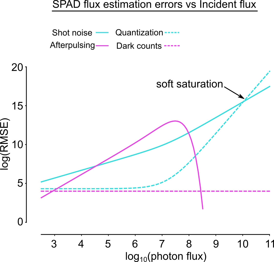
Various unique properties of the shot noise and quantization noise were discussed in the main text. Another surprising result is that the effect of afterpulsing bias first increases and then decreases with incident photon flux. Recall that afterpulses are correlated with past avalanche events. At very low incident photon flux there are very few photon-induced avalanches which implies that there are even fewer afterpulsing avalanches. At very high photon flux values, the afterpulsing noise is overwhelmed by the large number of true photon-induced avalanches that leave negligible temporal gaps between consecutive dead time windows. However, for most modern SPAD pixels, afterpulsing noise is so small that it can often be ignored. The plot in Supplementary Figure 1 shows an afterpulsing error curve using an unrealistically high afterpulsing rate to accentuate the trend as a function of incident flux.

Supplementary Figure 1: Effect of various sources of noise on the estimated photon flux for a conventional and a SPAD pixel. This figure shows the contributions to the flux estimation error from various sources of noise in a SPAD pixel. Quantization noise and shot noise were discussed in the main text and in Figure 3. Bias due to afterpulsing noise increases with incident flux and then decreases. Dark count noise remains small and constant at all flux levels. In order to accentuate the trend of afterpulsing error with incident flux, this plot uses an unrealistically high afterpulsing probability of 30%, which is much higher than the 1% probability for our hardware prototype.

Supplementary Note 5 SNR of a Conventional Sensor Pixel

A conventional CCD or CMOS pixel suffers from a hard saturation limit due to its full well capacity, $N_{\mathrm{FWC}}$. Assuming a quantum efficiency of $0<q<1$, an incident photon flux of $\Phi$ photons/second and an exposure time $T$ seconds, the photon counts $N_{T}$ follow a Gaussian distribution with mean $q\Phi T$ and variance $q\Phi T+\sigma_{r}^{2}$ where $\sigma_{r}$ is the read noise of the pixel. The estimated flux is given by [7]:

$$\hat{\Phi}_{\text{CCD}}=\begin{cases}\frac{N_{T}}{qT},&N_{T}<N_{\mathrm{FWC}}\\ \infty,&N_{T}=N_{\mathrm{FWC}}.\end{cases}$$

The RMSE of the estimated flux is given by:

$$\mathsf{RMSE}(\hat{\Phi}_{\text{CCD}})=\sqrt{\mathbf{E}[(\hat{\Phi}_{\text{CCD}}-\Phi)^{2}]}=\begin{cases}\frac{\sqrt{q\Phi T+\sigma_{r}^{2}}}{qT},&\Phi<\frac{N_{\mathrm{FWC}}}{qT}\\ \infty,&\Phi\geq\frac{N_{\mathrm{FWC}}}{qT}.\end{cases}$$

which leads to the following formula for SNR of conventional pixel:

$$\mathsf{SNR}_{\textrm{CCD}}(\Phi)=\begin{cases}10\log_{10}\left(\frac{q^{2}\Phi^{2}T^{2}}{q\Phi T+\sigma_{r}^{2}}\right),&\Phi<\frac{N_{\mathrm{FWC}}}{qT}\\ -\infty,&\Phi\geq\frac{N_{\mathrm{FWC}}}{qT}.\end{cases}$$ (S13)

This formula does not account for dark current noise because it is only relevent at extremely low incident photon flux values with very long exposure times of many minutes or longer.

Supplementary Note 6 Effect of Varying Exposure Time

The notions of quantum efficiency and exposure time are interchangeable in case of conventional image sensors; Equation (S13) remains unchanged if the symbols $q$ and $T$ were to be swapped. This is not true for a PF-SPAD sensor where changing $q$ and changing $T$ has different effects on the overall SNR. This is because the SPAD pixel has an asymptotic saturation limit of $T/\tau_{d}$ counts which is a function of exposure time, unlike a conventional sensor whose full well capacity is a fixed constant independent of exposure time. As shown in Supplementary Figure 2, decreasing exposure time decreases the maximum achievable SNR value of a SPAD sensor. Experimental results were obtained from our hardware prototype using a dead time of $300\text{\,}\mathrm{ns}$ and capturing photon counts with two different exposure times of $0.5\text{\,}\mathrm{ms}$ and $$5\text{\,}\mathrm{ms}$.$

Supplementary Figure 2: Effect of varying exposure time on SNR (a) For a conventional sensor, decreasing exposure time translates the SNR curve towards higher photon flux values while keeping the overall shape of the curve same. However, for a PF-SPAD pixel, decreasing exposure time decreases the maximum achievable SNR. (b) Experimental SNR data obtained with two exposure times. The SNR curves decay more rapidly than (a) due to additional dead time uncertainty effects in our hardware prototype, but the decrease in maximum achievable SNR is still clearly seen.

Supplementary Note 7 Details of SPAD Simulation Model and Experimental Setup

We implemented a time-domain simulation model for a PF-SPAD pixel to validate our theoretical formulas for the PF-SPAD response curve and SNR. Photons impinge the simulated PF-SPAD pixel according to a Poisson process; a fraction of these photons are missed due to limited quantum efficiency. The PF-SPAD pixel counts an incident photon when it arrives outside a dead time window. The simulation model also accounts for spurious detection events to dark counts and afterpulsing. The pseudo-code is shown in Supplementary Figure 3.

PF-SPAD and Conventional Sensor Specifications

Each pixel in the simulated PF-SPAD array mimics the specifications of the single-pixel hardware prototype. Each pixel in our simulated conventional sensor array uses slightly higher specifications than the one we used in our experiments. It has a full well capacity of 33,400 electrons, quantum efficiency of 90% and read noise of 5 electrons.

The single-pixel SPAD simulator was used for generating synthetic color images from a hypothetical megapixel SPAD array camera. The ground truth photon flux values were obtained from an exposure bracketed HDR image that covered over 10 orders of magnitude in dynamic range. Unlike regular digital images that use 8 bit integers for each pixel value, an HDR image is represented using floating point values that represent the true scene radiance at each pixel. These floating point values were appropriately scaled and used as the ground-truth photon flux to generate a sequence of photon arrival times following Poisson process statistics. Red, green and blue color channels were simulated independently. Results of simulated HDR images are shown in Supplementary Figures 7, 8 and 9.

1:$\;\,\Phi$: true incident photon flux $T$: exposure time $q$: SPAD pixel photon detection probability (quantum efficiency) $\Phi_{\mathrm{dark}}$: SPAD dark count rate $\tau_{d}$: dead time $p_{\mathrm{ap}}$: afterpulsing probability

2:$N_{T}$: number of photon detections

3:procedure PFSPADSimulator($\Phi,T,q,\tau_{d},p_{\mathrm{ap}}$)

4:     Reset number of photon detections $N_{T}\leftarrow 0$

5:     Reset last detection time $t_{\mathrm{last}}\leftarrow-\infty$

6:     Reset simulation time $t\leftarrow 0$

7:     Initialize afterpulse time-stamp array $\mathbf{t}_{\mathrm{ap}}=[\,]$

8:     while $t\leq T$ do

9:         Process timestamps in the after-pulsing time vector $\mathbf{t}_{\mathrm{ap}}$

10:         Generate next photon time-stamp $t\leftarrow t+\mathrm{Exp}(q\Phi+\Phi_{\mathrm{dark}})$

11:         if $t\geq t_{\mathrm{last}}+\tau_{d}$ then

12:              Append next afterpulse time-stamp to $\mathbf{t}_{\mathrm{ap}}$

13:              $N_{T}\leftarrow N_{T}+1$

14:              $t_{\mathrm{last}}\leftarrow t$

15:         end if

16:     end while

17:end procedure

Supplementary Figure 3: Computational model of a PF-SPAD pixel.

Supplementary Figure 4: Experimental setup for raster scanning with a single-pixel PF-SPAD sensor. (a) The setup consists of a SPAD module mounted on two translation stages, and a variable focal length lens that relays the imaged scene onto the image plane. Photon counts are captured using a free-running time-correlated single-photon counting module operated without a synchronization signal. (b) A picture of our SPAD sensor mounted on the translatation stages.

Experimental Setup Details

The single-pixel SPAD from our hardware prototype has a pitch of $25\text{\,}\mathrm{\SIUnitSymbolMicro m}$, quantum efficiency of 40%, dark count rate of 100 photons/second and 1% afterpulsing probability. The dead time is programmable and was set to $149.7\text{\,}\mathrm{ns}$ and exposure time to $5\text{\,}\mathrm{ms}$. This corresponds to an asymptotic saturation limit of 33,400 photons.

Each pixel in our machine vision camera (Point Grey GS3-U3-23S6M-C) has a full well capacity of 32,513 electrons, a peak quantum efficiency of 80% and a Gaussian-distributed read noise with a standard deviation of 6.83 electrons. Note that the asymptotic saturation limit of the PF-SPAD pixel is similar to the full well capacity of this machine vision camera to enable fair comparison.

Supplementary Note 8 Effect of Dead Time Jitter

In practice the dead time window is controlled using digital timer circuits that have a limited precision dictated by the clock speed. The hardware used in our experiments has a clock speed of 167 MHz which introduces a variance of $6\text{\,}\mathrm{ns}$ in the duration of the dead time window. As a result the dead time $\tau_{d}$ can no longer be treated as a constant but must be treated as a random variable $T_{d}$ with mean $\mu_{d}$ and variance $\sigma_{d}.$ The inter-arrival distribution in Equation (S1) must be understood as a conditional distribution, conditioned on $T_{d}=\tau_{d}$. The mean and variance of the time between photon detections can be computed using the law of iterated expectation [6]:

$$\mathbf{E}[X_{n}]=\mathbf{E}[\mathbf{E}[X_{n}|T_{d}]]=\mu_{d}+\frac{1}{q\Phi}$$

and

$$\mathrm{Var}[X_{n}]=\mathbf{E}[(X_{n}-\mathbf{E}[X_{n}])^{2}]=\mathbf{E}[\mathbf{E}[(X_{n}-\mathbf{E}[\mathbf{E}[X_{n}|\mathrm{T}_{d}]])^{2}|\mathrm{T}_{d}]]=1/q^{2}\Phi^{2}+\sigma_{d}^{2}.$$

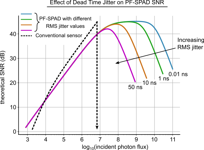
Using similar computations as those leading to Equation (S8), we can derive a modified shot noise variance term equal to $\frac{\Phi(1+q^{2}\Phi^{2}\sigma_{d}^{2})(1+q\Phi\mu_{d})}{qT}$ that must be used in Equation (S10) to account for dead time variance. All instances of $\tau_{d}$ in Equation (S10) must be replaced by its mean value $\mu_{d}$. Supplementary Figure 5 shows theoretical SNR curves for a PF-SPAD pixel with a nominal dead time duration of $149.7\text{\,}\mathrm{ns}$. Observe that the 30 dB dynamic range degrades by almost 3 orders of magnitude when the dead time jitter increases from $0.01\text{\,}\mathrm{ns}$ to $50\text{\,}\mathrm{ns}$. For reference, our hardware prototype has a dead time jitter of $6\text{\,}\mathrm{ns}$ RMS.

Supplementary Figure 5: Effect of dead time jitter on PF-SPAD SNR This figure shows theoretical effect of different values of dead time jitter on the PF-SPAD’s SNR is shown. (5 ms exposure time, 149.7 ns dead time, 40% quantum efficiency and 100 Hz dark count rate.)

Supplementary Note 9 Comparison with Quanta Image Sensors

A quanta image sensor (QIS) [4,5,8] improves dynamic range by spatially oversampling the 2D scene intensities using sub-diffraction limit sized pixels called jots. Each jot has a limited full well capacity, usually just one photo-electron. The PF-SPAD imaging modality presented in this paper is different from these methods. Instead of using a SPAD as a binary pixel [4] and relying on spatial oversampling, the PF-SPAD achieves dynamic range compression by allowing the dead time windows to shift randomly based on the most recent photon detection time and performing adaptive photon rejection. This is equivalent to the “event-driven recharge” method described in [2].

We now derive the image formation model and an expression for SNR for a QIS and other related methods that use equi-spaced time bins [8], and show that their dynamic range is lower than what can be achieved using a PF-SPAD.

QIS Image Formation and Flux Estimator

The output response of a QIS is logarithmic and mimics silver halide photographic film [5]. Each jot has a binary output, and the final image is formed by spatio-temporally combining groups of jots called a “jot-cube”. Let $\tau_{b}$ be the temporal bin width and for mathematical convenience, assume that the exposure time $T$ is an integer multiple of $\tau_{b}$, so that there are $N=T/\tau_{b}$ uniformly spaced time bins that split the total exposure duration. Suppose the jot-cube is exposed to a constant photon flux of $\Phi$ photons/second, and each jot has a quantum efficiency $0<q<1$. The number of photons received by each jot in a time interval $\tau_{b}$ follows a Poisson distribution with mean $q\Phi\tau_{b}$. Therefore the probability that the binary output of a jot is $0$ is given by:

$$\mathsf{Pr}(\mathrm{jot=0})=e^{-q\Phi\tau_{b}}$$

and the probability that the binary output of a jot is $1$ is given by the probability of observing $1$ or more photons:

$$\mathsf{Pr}(\mathrm{jot=1})=1-e^{-q\Phi\tau_{b}}.$$

Let $N_{T}$ denote the total photon counts output from a jot-cube with $N$ jots. Then $N_{T}$ follows a binomial distribution given by:

$$\mathsf{Pr}(N_{T}=k)=\binom{N}{k}(1-e^{-q\Phi\tau_{b}})^{k}(e^{-q\Phi\tau_{b}})^{N-k},$$

for $0\leq k\leq N$. The maximum-likelihood estimate of the photon flux is given by:

$$\hat{\Phi}_{\textrm{QIS}}=\frac{1}{q\tau_{b}}\log\left(\frac{T}{T-N_{T}\tau_{b}}\right).$$ (S14)

Our PF-SPAD flux extimator has a higher dynamic range than this uniform binning method. This can be intuitively understood by noting that in the limiting case of $\tau_{b}=\tau_{d}$ both schemes have an upper limit on photon counts given by $N_{T}\leq T/\tau_{d},$ but the QIS estimator in Equation (S14) saturates and flattens out more rapidly than the PF-SPAD estimator in Equation (2) from the main text:

$$\frac{d\hat{\Phi}_{\textrm{QIS}}}{dN_{T}}=\frac{1}{q}\frac{1}{T-N_{T}\tau_{b}}<\frac{1}{q}\frac{T}{(T-N_{T}\tau_{d})^{2}}=\frac{d\hat{\Phi}}{dN_{T}}.$$

SNR of a QIS

The variance of the QIS flux estimator can be computed numerically using the binomial probability mass function of $N_{T}$. For convenience, a closed form expression can be derived using a Gaussian approximation, similar to the approximation techniques used for deriving the SNR of a PF-SPAD pixel in Equation (S8). The Gaussian approximation to a binomial distribution suggests $N_{T}$ has a normal distribution with mean $N\,(1-e^{-q\Phi\tau_{b}})$ and variance $N\,e^{-q\Phi\tau_{b}}(1-e^{-q\Phi\tau_{b}})$. Next, the c.d.f. of the estimated flux is given by:

$$F_{\hat{\Phi}_{\textrm{QIS}}}(x) =\mathsf{Pr}(\hat{\Phi}_{\textrm{QIS}}\leq x)$$

$$=\mathsf{Pr}\left(-\frac{1}{q\tau_{b}}\log\left(1-\frac{N_{T}}{N}\right)\leq x\right)$$

$$=\mathsf{Pr}(N_{T}\leq(1-e^{-xq\tau_{b}})N)$$

$$=\frac{1}{2}\left(1+\mathrm{erf}\left(\frac{N(1-e^{-xq\tau_{b}})-N(1-e^{-\Phi q\tau_{b}})}{\sqrt{2}\sqrt{N(1-e^{-\Phi q\tau_{b}})e^{-\Phi q\tau_{b}}}}\right)\right)$$ (S15)

$$\approx\frac{1}{2}\left(1+\mathrm{erf}\left(\sqrt{N}\frac{(x-\Phi)e^{-\Phi q\tau_{b}}q\tau_{b}}{\sqrt{2(1-e^{-\Phi q\tau_{b}})e^{-\Phi q\tau_{b}}}}\right)\right)$$ (S16)

$$=\frac{1}{2}\left(\mathrm{1+erf}\left(\frac{x-\Phi}{\sqrt{2}\sqrt{\frac{(1-e^{-\Phi q\tau_{b}})}{q^{2}T\tau_{b}e^{-\Phi q\tau_{b}}}}}\right)\right)$$ (S17)

where Equation (S15) follows from the formula for the c.d.f. of a Gaussian distribution and Equation (S16) is obtained after making a Taylor series approximation. The final form of Equation (S17) suggests that the estimated photon flux follows a normal distribution with variance $\frac{(1-e^{-\Phi q\tau_{b}})}{q^{2}T\tau_{b}e^{-\Phi q\tau_{b}}}.$

The read noise of each jot affects the RMSE of the QIS sensor at low incident flux. We note that at low flux values there are, on average, $q\Phi T$ bins already filled by true photon counts leaving $N-q\Phi T$ bins empty. Read noise will cause some of these empty bins to contain false positives and introduce additional noisy counts equal to $\frac{1}{2}(N-q\Phi T)\left(1+\mathrm{erf}\left(\frac{1}{2\sqrt{2}\sigma_{r}}\right)\right)$, where $\sigma_{r}$ is the read noise standard deviation. This corresponds to a bias of $\frac{1}{2}(\frac{1}{q\tau_{b}}-\Phi)\left(1-\mathrm{erf}\left(\frac{1}{2\sqrt{2}\sigma_{r}}\right)\right)$ in the estimated photon flux. Incorporating this bias term together with the variance associated with the Gaussian distribution of the estimated photon flux, the RMSE is given by

$$\mathsf{RMSE}(\hat{\Phi}_{\textrm{QIS}})=\sqrt{\max\left\{0,\frac{1}{2}\left(\frac{1}{q\tau_{b}}-\Phi\right)\left(1-\mathrm{erf}\left(\frac{1}{2\sqrt{2}\sigma_{r}}\right)\right)\right\}^{2}+\frac{1-e^{-q\Phi\tau_{b}}}{q^{2}T\tau_{b}e^{-q\Phi\tau_{b}}}}.$$

Supplementary Figure 6: Theoretical SNR curves for a SPAD pixel compared to the effective SNR of a QIS jot block occupying the same area as the SPAD pixel. Each QIS jot has a read noise standard deviation of 0.13 electrons and quantum efficiency of 80%. The SPAD pixel has a dead time of $150\text{\,}\mathrm{ns}$, dark count rate of 100 photons/s, 40% quantum efficiency and 1% afterpulsing rate. A fixed exposure time of $5\text{\,}\mathrm{ms}$ is assumed for both types of pixels. Sub-diffraction limit jot sizes of under $150\text{\,}\mathrm{nm}$ will be required to obtain similar dynamic range as a single $25\text{\,}\mathrm{\SIUnitSymbolMicro m}$ SPAD pixel.

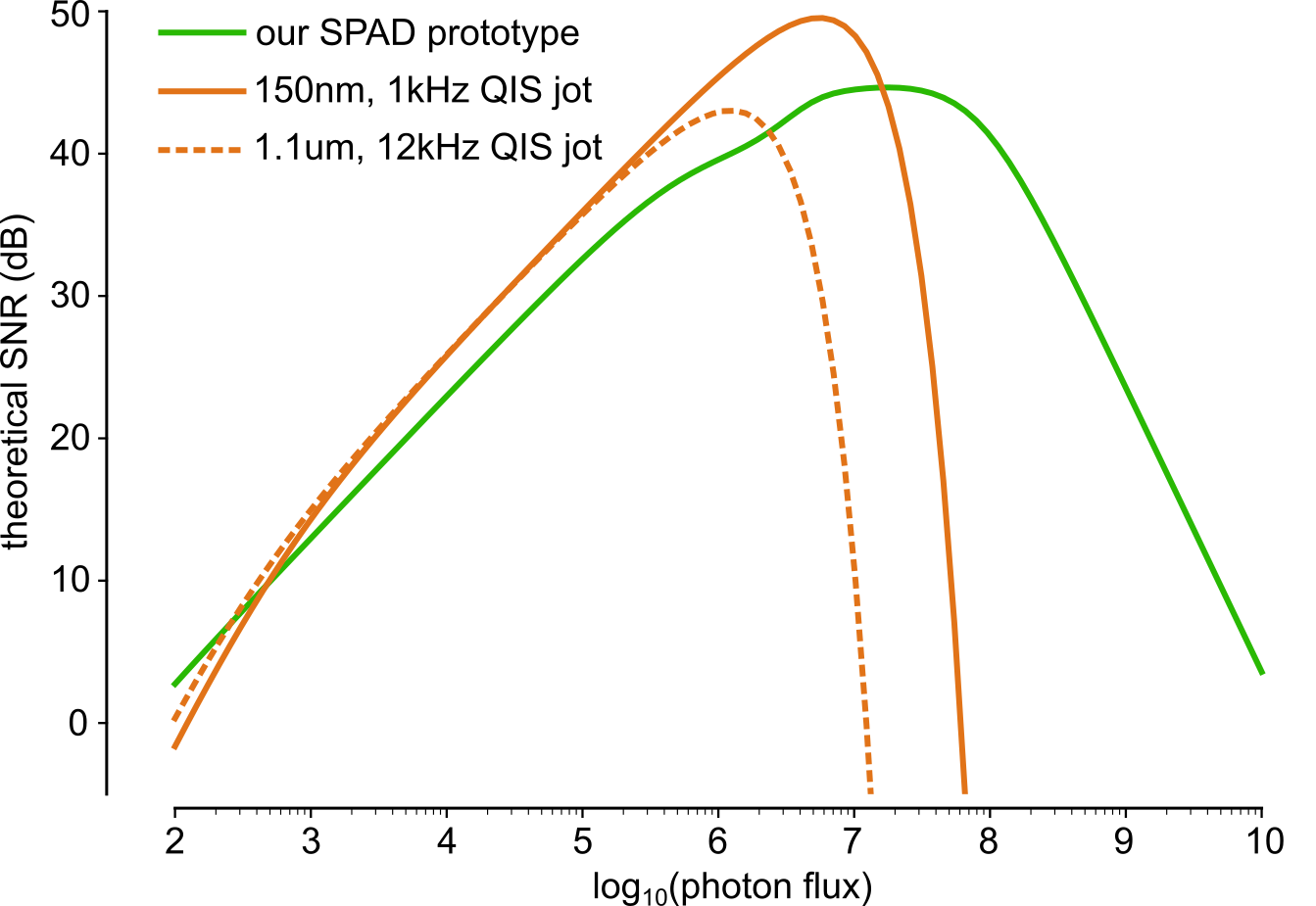
A single jot only generates a binary output and must be combined into a jot-cube to generate the final image. One way to obtain a fair comparison between a PF-SPAD pixel and a jot-cube is computing the SNR for a fixed image pixel size and fixed exposure time. We use a square grid of jots that spatially occupy the same area as our single PF-SPAD pixel that has a pitch of $25\text{\,}\mathrm{\SIUnitSymbolMicro m}$. Supplementary Figure 6 shows the SNR curves obtained using our theoretical derivations for a QIS jot-cube and a single PF-SPAD pixel. State of the art jot arrays are limited to a pixel size of around $1\text{\,}\mathrm{\SIUnitSymbolMicro m}$ and frame rates of a few kHz. These SNR curves show that we will require large spatio-temporal oversampling factors and extremely small jots to obtain similar dynamic range as a single PF-SPAD pixel. For example, a $150\text{\,}\mathrm{nm}$ jot size can accommodate almost 30,000 jots in a $25\times$$25\text{\,}\mathrm{\SIUnitSymbolMicro m}$² area occupied by the PF-SPAD pixel and can provide similar dynamic range and higher SNR than our PF-SPAD pixel when operated at a frame rate of 1 kHz. QIS technology will require an order of magnitude increase in frame readout rate or an order of magnitude reduction in jot size to bring it closer to the dynamic range achievable with our PF-SPAD prototype.

Supplementary Note 10 Additional Simulated and Experimental Results

Supplementary Figure 7: Simulation-based comparison of a conventional image sensor and a PF-SPAD on a high dynamic range scene. The ground truth high dynamic range image was obtained using a DSLR camera with exposure bracketing over 10 stops. (a) Simulated $5\text{\,}\mathrm{ms}$ exposure image of the scene obtained using a conventional camera sensor. (b) Simulated $50\text{\,}\mathrm{\SIUnitSymbolMicro s}$ exposure time image using a conventional camera. (c) Simulated SPAD image of the same scene acquired with a single $5\text{\,}\mathrm{ms}$ exposure captures the full dynamic range in a single shot. Identical tone-mapping was applied to all images and zoomed insets for a fair comparison and reliable visualization of the entire dynamic range.

Supplementary Figure 8: Simulated outdoor HDR scene. (a) Long exposure capture using a conventional camera captures darker regions of the scene but the regions around the sun are saturated. (b) Short exposure time capture using a conventional sensor prevents the sun-lit region from appearing saturated but results in lost information in the shadows. (c) A single capture using a simulated PF-SPAD array circumvents the problem of low dynamic range by simultaneously capturing both highlights and shadows. Original HDR image was obtained from the sIBL datasets website www.hdrlabs.com/sibl/archive.html.

Supplementary Figure 9: Simulated indoor HDR scene. (a) Long exposure capture using a conventional camera captures darker regions of the scene but the regions around the bulb are completely saturated. (b) Short exposure time capture using a conventional sensor shows details of bulb filament but darker regions of the scene appear grainy due to underexposure. (c) A single capture using a PF-SPAD captures both bright and dark regions simultaneously. The original HDR image was captured using a Canon EOS Rebel T5 DSLR camera with 10 stops and rescaled to cover $10^{6}:1$ dynamic range.

Supplementary Figure 10: Comparison of the dynamic range of images captured using a conventional camera and our PF-SPAD hardware prototype. (a) Long exposure ($5\text{\,}\mathrm{ms}$) shot using a conventional camera captures darker regions of the scene such as the text but the regions around the bulb filaments appear saturated. (b) Short exposure time ($0.5\text{\,}\mathrm{ms}$) capture using a shows filaments of all bulbs but leaves the darker part of the scene such as the book underexposed. (c) A single $5\text{\,}\mathrm{ms}$ exposure shot using the SPAD prototype captures the entire dynamic range. The bright bulb filament and dark text on the book are simultaneously visible.

Supplementary References

1. Abramowitz, M. & Stegun, I. A. Handbook of Mathematical Functions: With Formulas, Graphs, and Mathematical Tables, vol. 55 (Dover American Nurses Association Publications, 1964), 9 edn.

2. Antolovic, I. M., Bruschini, C. & Charbon, E. Dynamic range extension for photon counting arrays. Optics Express 26, 22234–22248 (2018).

3. Casella, G. & Berger, R. L. Statistical Inference (Pacific Grove, CA: Duxbury/Thomson Learning, 2002), 2nd edn. Sec. 5.5.4.

4. Dutton, N. A. W. et al. A SPAD-based QVGA image sensor for single-photon counting and quanta imaging. IEEE Transactions on Electron Devices 63, 189–196 (2016).

5. Fossum, E., Ma, J., Masoodian, S., Anzagira, L. & Zizza, R. The quanta image sensor: Every photon counts. Sensors 16, 1260 (2016).

6. Grimmett, G. R. & Stirzaker, D. R. Probability and Random Processes (Oxford University Press, 2001), 3rd edn.

7. Hasinoff, S. W. et al. Noise-Optimal Capture for High Dynamic Range Photography. Proc. 23rd IEEE Conference on Computer Vision and Pattern Recognition (CVPR), pp. 553–560 (2010).

8. Itzler, M. A. Apparatus comprising a high dynamic range single-photon passive 2D imager and methods therefor (2017).

References

- [1] S. Cova, M. Ghioni, A. Lacaita, C. Samori, and F. Zappa, “Avalanche photodiodes and quenching circuits for single-photon detection,” Appl. Opt., vol. 35, pp. 1956–1976, Apr 1996.
- [2] T. Niehörster, A. Löschberger, I. Gregor, B. Krämer, H.-J. Rahn, M. Patting, F. Koberling, J. Enderlein, and M. Sauer, “Multi-target spectrally resolved fluorescence lifetime imaging microscopy,” Nature methods, vol. 13, no. 3, p. 257, 2016.
- [3] I. M. Antolovic, S. Burri, C. Bruschini, R. A. Hoebe, and E. Charbon, “SPAD imagers for super resolution localization microscopy enable analysis of fast fluorophore blinking,” Scientific Reports, vol. 7, p. 44108, Mar 2017.
- [4] Y. Altmann, S. McLaughlin, M. J. Padgett, V. K. Goyal, A. O. Hero, and D. Faccio, “Quantum-inspired computational imaging,” Science, vol. 361, no. 6403, 2018.
- [5] A. Kirmani, D. Venkatraman, D. Shin, A. Colaço, F. N. C. Wong, J. H. Shapiro, and V. K. Goyal, “First-photon imaging,” Science, vol. 343, no. 6166, pp. 58–61, 2014.
- [6] D. Shin, F. Xu, D. Venkatraman, R. Lussana, F. Villa, F. Zappa, V. K. Goyal, F. N. C. Wong, and J. H. Shapiro, “Photon-efficient imaging with a single-photon camera,” Nature Communications, vol. 7, p. 12046, Jun 2016.
- [7] M. Buttafava, J. Zeman, A. Tosi, K. Eliceiri, and A. Velten, “Non-line-of-sight imaging using a time-gated single photon avalanche diode,” Opt. Express, vol. 23, pp. 20997–21011, Aug 2015.
- [8] G. Gariepy, F. Tonolini, R. Henderson, J. Leach, and D. Faccio, “Detection and tracking of moving objects hidden from view,” Nature Photonics, vol. 10, pp. 23–26, 2016.
- [9] M. O’Toole, D. B. Lindell, and G. Wetzstein, “Confocal non-line-of-sight imaging based on the light-cone transform,” Nature, vol. 555, pp. 338–341, Mar 2018.
- [10] A. E. Gamal and H. Eltoukhy, “CMOS image sensors,” IEEE Circuits and Devices Magazine, vol. 21, pp. 6–20, May 2005.
- [11] H. P. Robinson, “On printing photographic pictures from several negatives,” British Journal of Photography, vol. 7, no. 115, p. 94, 1860.
- [12] P. E. Debevec and J. Malik, “Recovering high dynamic range radiance maps from photographs,” in ACM SIGGRAPH 2008, (Los Angeles, CA), p. 31, 2008.
- [13] M. Gupta, D. Iso, and S. K. Nayar, “Fibonacci exposure bracketing for high dynamic range imaging,” in 2013 IEEE International Conference on Computer Vision, (Sydney, Australia), pp. 1473–1480, Dec 2013.
- [14] S. Nayar and T. Mitsunaga, “High dynamic range imaging: spatially varying pixel exposures,” in Proceedings IEEE Conference on Computer Vision and Pattern Recognition CVPR 2000, (Hilton Head, SC), pp. 472–479, IEEE Comput. Soc, 2000.
- [15] Nayar and Branzoi, “Adaptive dynamic range imaging: optical control of pixel exposures over space and time,” in Proceedings Ninth IEEE International Conference on Computer Vision, IEEE, 2003.
- [16] M. D. Tocci, C. Kiser, N. Tocci, and P. Sen, “A versatile HDR video production system,” ACM Transactions on Graphics (TOG), vol. 30, no. 4, p. 41, 2011.
- [17] S. Kavadias, B. Dierickx, D. Scheffer, A. Alaerts, D. Uwaerts, and J. Bogaerts, “A logarithmic response cmos image sensor with on-chip calibration,” IEEE Journal of Solid-State Circuits, vol. 35, pp. 1146–1152, Aug 2000.
- [18] F. Yang, Y. M. Lu, L. Sbaiz, and M. Vetterli, “Bits from photons: Oversampled image acquisition using binary poisson statistics,” IEEE Transactions on Image Processing, vol. 21, pp. 1421–1436, Apr 2012.
- [19] E. Fossum, J. Ma, S. Masoodian, L. Anzagira, and R. Zizza, “The quanta image sensor: Every photon counts,” Sensors, vol. 16, p. 1260, Aug 2016.
- [20] N. A. W. Dutton, I. Gyongy, L. Parmesan, S. Gnecchi, N. Calder, B. R. Rae, S. Pellegrini, L. A. Grant, and R. K. Henderson, “A SPAD-based QVGA image sensor for single-photon counting and quanta imaging,” IEEE Transactions on Electron Devices, vol. 63, pp. 189–196, Jan 2016.
- [21] I. M. Antolovic, C. Bruschini, and E. Charbon, “Dynamic range extension for photon counting arrays,” Optics Express, vol. 26, pp. 22234–22248, Aug 2018.
- [22] S. W. Hasinoff and K. Ikeuchi, Photon, Poisson Noise, pp. 608–610. Boston, MA: Springer US, 2014.
- [23] J. W. Müller, “Dead-time problems,” Nuclear Instruments and Methods, vol. 112, no. 1-2, pp. 47–57, 1973.
- [24] G. R. Grimmett and D. R. Stirzaker, Probability and Random Processes. Oxford University Press, 3 ed., 2001.
- [25] H. R. Blackwell, “Contrast thresholds of the human eye,” Journal of the Optical Society of America, vol. 36, p. 624, Nov 1946.
- [26] J. N. Tinsley, M. I. Molodtsov, R. Prevedel, D. Wartmann, J. Espigulé-Pons, M. Lauwers, and A. Vaziri, “Direct detection of a single photon by humans,” Nature Communications, vol. 7, p. 12172, Jul 2016.
- [27] C. Marois, B. Macintosh, T. Barman, B. Zuckerman, I. Song, J. Patience, D. Lafreniere, and R. Doyon, “Direct imaging of multiple planets orbiting the star HR 8799,” Science, vol. 322, pp. 1348–1352, Nov 2008.
- [28] D. J. Brady, M. E. Gehm, R. A. Stack, D. L. Marks, D. S. Kittle, D. R. Golish, E. M. Vera, and S. D. Feller, “Multiscale gigapixel photography,” Nature, vol. 486, pp. 386–389, Jun 2012.
- [29] C. Vinegoni, C. L. Swisher, P. F. Feruglio, R. J. Giedt, D. L. Rousso, S. Stapleton, and R. Weissleder, “Real-time high dynamic range laser scanning microscopy,” Nature Communications, vol. 7, p. 11077, Apr 2016.
- [30] F. D. I. and O. A. S., “Using multiple exposures to improve image processing for autonomous vehicles,” May 2017.
- [31] M. A. Itzler, “Apparatus comprising a high dynamic range single-photon passive 2D imager and methods therefor,” Mar 2017.
- [32] N. Roy, F. Nolet, F. Dubois, M. O. Mercier, R. Fontaine, and J. F. Pratte, “Low power and small area, 6.9 ps rms time-to-digital converter for 3d digital sipm,” IEEE Transactions on Radiation and Plasma Medical Sciences, vol. 1, no. 6, pp. 486–494, 2017.
- [33] I. Gyongy, N. Calder, A. Davies, N. A. Dutton, R. R. Duncan, C. Rickman, P. Dalgarno, and R. K. Henderson, “A 256x256, 100-kfps, 61% Fill-Factor SPAD Image Sensor for Time-Resolved Microscopy Applications,” IEEE Transactions on Electron Devices, vol. 65, no. 2, pp. 547–554, 2018.
Supplementary Document for