Electromagnetic multipole moments of baryons

Abstract

We calculate the charge quadrupole and magnetic octupole moments of baryons using a group theoretical approach based on broken SU(6) spin-flavor symmetry. The latter is an approximate symmetry of the QCD Lagrangian which becomes exact in the large color $N_{c}$ limit. Spin-flavor symmetry breaking is induced by one-, two-, and three-quark terms in the electromagnetic current operator. Two- and three-quark currents provide the leading contributions for higher multipole moments, despite being of higher order in an $1/N_{c}$ expansion. Our formalism leads to relations between $N\to N^{*}$ transition multipole moments and nucleon ground state properties. We compare our results to experimental quadrupole and octupole transition moments extracted from measured helicity amplitudes.

I Introduction

Electromagnetic multipole moments of baryons are interesting observables. They are directly connected with the spatial charge and current distributions in baryons, and thus contain information about their size, shape, and internal structure. In particular, charge quadrupole and magnetic octupole moments provide important information on the geometric shape of baryons, which is not available from the corresponding leading multipole moments.

However, higher electromagnetic multipole moments, such as charge quadrupole (C2) and magnetic octupole (M3) moments of spin $\geq 3/2$ baryons are very difficult to measure. Presently, we have no direct experimental information on these moments, but it is planned to measure the quadrupole moment of the $\Omega^{-}$ baryon at FAIR in DarmstadtPoc17 . This is contrasted by several theoretical works on baryon quadrupole moments But94 ; Leb95 ; Oh95 ; Hen01 ; Hes02 ; Dah13 ; Kri91 ; Ram09 ; Gia90 and relatively few on magnetic octupole moments Ram09 ; Gia90 ; Buc08 ; Ali09 .

On the other hand, transition multipole moments between the ground state and excited states of the nucleon as shown in Fig. 1 are experimentally accessible. High precision electron and photon scattering experiments, exciting the lowest lying nucleon resonance $\Delta^{+}(1232)$ have provided evidence for a nonzero $p\to\Delta^{+}$ transition quadrupole moment $Q_{p\to\Delta^{+}}$ and hence for a nonspherical charge distribution in baryons. The experimental results Tia03 ; Bla01 are in agreement with the quark model prediction BHF97

$$Q_{p\to\Delta^{+}}=\frac{1}{\sqrt{2}}\,r_{n}^{2},$$ (1)

where $r_{n}^{2}$ is the neutron charge radius Kop97 . It has been suggested that a transition quadrupole moment of the sign as in Eq.(1) arises because the proton has a prolate and the $\Delta^{+}$ an oblate charge distribution and that the neutron charge radius is a measure of the intrinsic quadrupole moment of the nucleon Hen01 . For reviews see Ref. Pas07 ; Ber07 .

Furthermore, it was proposed Buc04 that Eq.(1) is the zero momentum transfer limit of a more general relation between the $p\to\Delta^{+}$ charge quadrupole transition form factor $G_{C2}^{p\to\Delta^{+}}(Q^{2})$ and the elastic neutron charge form factor $G_{C}^{n}(Q^{2})$

$$G_{C2}^{p\to\Delta^{+}}(Q^{2})=-\frac{3\sqrt{2}}{Q^{2}}\,G_{C}^{n}(Q^{2}).$$ (2)

Eq.(2) agrees with experiment for a wide range of momentum transfers. In addition, it has the correct low $Q^{2}$ behavior of a charge quadrupole form factor, and the correct high $Q^{2}$ asymptotic behavior predicted by perturbative QCD Idi04 ; Tia07 ; tia16 .

The purpose of the present contribution is to further explore relations between transition multipole moments and nucleon ground state properties. We will focus our attention on the Coulomb quadrupole (C2) and magnetic octupole (M3) transition form factors as shown in Fig. 1. The reason for this is that these are next-to-leading moments of the elastic charge monopole (C0) and magnetic dipole (M1) nucleon form factors. While the nucleon ground state does not have spectroscopic quadrupole and octupole moments, it does have corresponding intrinsic moments. We will extract the sign and size of these intrinsic ground state moments from the measurable transition moments and discuss their implications for the shape of the nucleon.

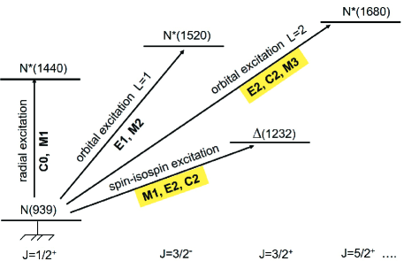
Figure 1: Low-lying nucleon resonances and transition multipole moments M, E, C.

II Electromagnetic excitation of nucleon resonances

II.1 Elastic and inelastic electron-nucleon scattering

On the way towards reaching a better understanding of the nucleon spectrum, meson electroproduction experiments depicted in Fig. 2(right) have been particularly fruitful. For recent reviews see Tia11 ; Azn11 . From the theory side, the electromagnetic structure of the nucleon is described in terms of elastic and inelastic multipole form factors as indicated in Fig. 2. The elastic form factors can to a certain extent be interpreted as Fourier transforms of the charge $\rho({\bf r})$ and spatial current distributions ${\bf J}({\bf r})$ inside the nucleon. Thus, the elastic form factors are directly related to the spatial structure of the nucleon ground state, which in turn determines the transition form factors to excited nucleon states.

Quite generally, the geometric properties of the ground state of a physical system, in particular its size and shape, have a direct bearing on the eigenfrequencies and eigenmodes of its excitation spectrum. Conversely, knowledge of the eigenfrequencies and excitation modes of a system enables us to draw certain conclusions concerning its size and shape. This also applies to the nucleon and suggests that e.g. the $N\to\Delta$ charge quadrupole (C2) transition form factor provides details about the nucleon ground state structure such as the quadrupole part of the charge density qualitatively illustrated in Fig. 3.

When trying to make inferences about the structure of a physical system based on the excitation spectrum and transition multipoles to various excited states, the symmetries respected by the system provide valuable guidance. The regularities seen in the excitation spectrum and other observables of a quantum mechanical system are usually due to an underlying symmetry and thus call for a group-theoretical treatment. An early example is the explanation of the orbital angular momentum $l$ degeneracy and the $1/n^{2}$ law in the spectrum of atomic hydrogen by Pauli and Fock Pau26 . Both properties were shown to follow from an underlying SO(4)$\sim$SU(2)${}_{V}\times$SU(2)_A symmetry that is isomorphic to the direct product of two SU(2) groups connected with two conserved quantities, orbital angular momentum (A) and the Lenz-Runge vector (V) Gre94 .

In the case of baryons, SU(2) isospin symmetry, as well as the higher flavor SU(3)_F and spin-flavor SU(6)_SF symmetries and their breaking provide useful guidelines not only for the classification of states but also for extracting information on baryon structure from electromagnetic multipoles. We will discuss the symmetry properties of electromagnetic multipoles in some detail in Sect. II.2 and Sect. III.

Figure 2: Left: Elastic electron-nucleon scattering $e\,N\to e^{\prime}\,N^{\prime}$ involving the exchange of a single virtual photon $\gamma$ of four-momentum $Q$, with $Q^{2}=-(\omega^{2}-{\bf q}^{2})$. Here, $\omega$ is the energy transfer and ${\bf q}$ the three-momentum transfer of the virtual photon. The nucleon structure information is contained in the charge monopole form factor $G^{N}_{C}(Q^{2})$ and magnetic dipole form factor $G^{N}_{M}(Q^{2})$. Right: Inelastic electron-nucleon scattering $e\,N\to e^{\prime}\,\Delta$. The excitation of the $\Delta$ resonance is described by three electromagnetic transition form factors $G^{N\to\Delta}_{M1}(Q^{2})$, $G^{N\to\Delta}_{E2}(Q^{2})$, and $G^{N\to\Delta}_{C2}(Q^{2})$.

II.2 Multipole operators and form factors

Baryons are quantum mechanical systems with definite angular momentum and parity. It is therefore advantageous to describe their electromagnetic interaction in terms of electromagnetic multipole operators which transfer definite angular momentum $J$ and parity. Angular momentum and parity selection rules then greatly facilitate the evaluation of matrix elements. Usually, only a few multipoles suffice to obtain a satisfactory description of the charge $\rho$ and current ${\bf J}$ distributions of the system.

A multipole expansion of the baryon charge density $\rho({\bf q})$ into Coulomb multipole operators $T_{M}^{[C]J}(q)$ is then given as def66

$$\rho({\bf q})=4\pi\sum_{JM}i^{J}Y^{J}_{M}({\bf{\hat{q}}})\,T_{M}^{[C]J}(q).$$ (3)

Here, ${\bf q}$ is the three-momentum transfer of the virtual photon and $Y^{J}_{M}({\bf{\hat{q}}})$ is a spherical harmonic of multipolarity $J$ and projection $M$. The Coulomb multipole operator $T_{M}^{[C]J}(q)$ is a spherical tensor of rank $J$ and parity $(-1)^{J}$ that is calculated from the charge density as follows

$$T_{M}^{[C]J}(q)=\int j_{J}(qr)Y^{J}_{M}({\bf{\hat{r}}})\rho({\bf r})\,d^{3}{\bf r},$$ (4)

where $j_{J}(qr)$ is a spherical Bessel function of order $J$.

Analogously, the transverse current density is expanded into transverse electric $T_{\lambda}^{[E]J}(q)$ and magnetic $T_{\lambda}^{[M]J}(q)$ multipole operators, which are spherical tensors of rank $J$ with parity $(-1)^{J}$ and $(-1)^{J+1}$ respectively as def66

$${\bf J}_{\lambda}(q)=-\sqrt{2\pi}\sum_{J\geq 1}(-i)^{J}{\hat{J}}\left[\lambda\,T_{\lambda}^{[M]J}(q)+T_{\lambda}^{[E]J}(q)\right],$$ (5)

where $\lambda$ can take on the values $\lambda=\pm 1$ and ${\hat{J}}=\sqrt{2J+1}$. The transverse magnetic and electric multipole operators are defined in terms of the spatial current density as

$$T_{\lambda}^{[M]J}(q)\!\! = \!\!\int\!j_{J}(qr){\bf Y}^{(J1)J}_{\lambda}({\bf{\hat{r}}})\cdot{\bf J}({\bf r})\,d^{3}{\bf r}$$

$$T_{\lambda}^{[E]J}(q)\!\! = \!\!\frac{1}{q}\int\!{\mbox{\boldmath$\nabla$}}\times(j_{J}(qr){\bf Y}^{(J1)J}_{\lambda}({\bf{\hat{r}}}))\cdot{\bf J}({\bf r})\,d^{3}{\bf r},$$ (6)

where ${\bf Y}^{(J1)J}_{\lambda}({\bf{\hat{r}}})$ are vector spherical harmonics.

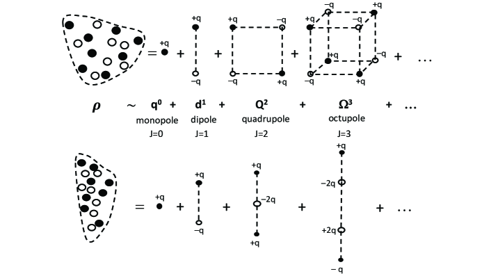
Figure 3: Qualitative illustration of the multipole expansion of classical charge densities $\rho$ into a series of Coulomb $2^{J}$-poles of multipolarity $J$. The different geometric shapes of $\rho$ are reflected by the sign and size of the higher multipole moments. Upper panel: oblate (pancake-shaped) $\rho$ with intrinsic quadrupole moment $Q_{0}<0$. Lower panel: prolate (cigar-shaped) $\rho$ with $Q_{0}>0$. Due to parity and time reversal invariance of the electromagnetic interaction only Coulomb multipole moments with even multipolarity are allowed quantum mechanically.

With angular momentum $J_{i}$ in the inital state and $J_{f}$ in the final state, angular momentum conservation restricts the number of multipole form factors of multipolarity $J$ as

$$|J_{i}-J_{f}|\leq J\leq J_{i}+J_{f}.$$ (7)

Furthermore, parity and time reversal invariance of the electromagnetic interaction implies that in elastic scattering, there can be only even charge multipoles and odd magnetic multipoles but no transverse electric multipoles. Specifically, for the positive parity nucleon ground state $N(939)$, the $\Delta(1232)$, and the $N^{*}(1680)$ resonance the allowed elastic and transition multipoles are listed in Table 1.

Table 1: Coulomb (C), magnetic (M) and electric (E) multipoles of multipolarity $J$ in elastic and inelastic electron-nucleon scattering for selected positive parity states.

state	elastic	transition
$N(939)$	C0, M1	—
$\Delta(1232)$	C0, C2	C2
	M1, M3	M1, E2
$N^{*}(1680)$	C0, C2, C4	C2
	M1, M3, M5	E2, M3

In general, the multipole operators depend on the photon three-momentum transfer $|{\bf q}|=q$, multipolarity $J$ and projection $M$. Their matrix elements give rise to corresponding transition multipole form factors def66

$$G^{N\to N^{*}}_{C0}\!\!(q^{2}) \!\!\!=\!\!\! \sqrt{4\pi}\,\langle N^{*}|T_{0}^{[C0]}(q)|N\rangle,$$

$$G^{N\to N^{*}}_{C2}\!\!(q^{2}) \!\!\!=\!\!\! \frac{12\sqrt{5\pi}}{q^{2}}\,\langle N^{*}|T_{0}^{[C2]}(q)|N\rangle,$$

$$\tilde{G}^{N\to N^{*}}_{M1}\!\!(q^{2}) \!\!\!=\!\!\! \frac{i\sqrt{6\pi}}{q}(2M_{N})\,\langle N^{*}|T_{0}^{[M1]}(q)|N\rangle,$$

$$\tilde{G}^{N\to N^{*}}_{M3}\!\!(q^{2}) \!\!\!=\!\!\! -\frac{i15\sqrt{21\pi}}{q^{3}}(2M_{N})\langle N^{*}|T_{0}^{[M3]}(q)|N\rangle,$$ (8)

where $N^{*}=N$ (elastic) and $N^{*}=\Delta(1232)$ or $N^{*}=N^{*}(1680)$ (inelastic). By convention, elastic and inelastic multipole form factors are evaluated for the $M=0$ projection of the multipole operator and the highest allowed total angular momentum projection of the baryon states involved.

In the present paper, we focus on the static multipole moments, which are the $q\to 0$ limit of the multipole form factors in Eq.(II.2). In this limit our multipole form factors are normalized to the usual spherical multipole moments known from classical electrodynamics Jac75 and are straightforward generalizations of the Sachs form factor normalization used in elastic scattering. In the $q\to 0$ limit we obtain from Eq.(II.2) and the definitions in Eq.(4) and Eq.(II.2) the total charge ${\rm Q}_{N}$ and magnetic moment $\tilde{{\mu}}_{N}$ in the elastic scattering case ($N^{*}=N$), in addition to the charge monopole and quadrupole as well as the magnetic dipole and octupole transition moments in inelastic scattering

$${\rm{Q}}_{N\to N^{*}}\!\! \!\!\!\!=\!\!\! G_{C0}^{N\to N^{*}}(0)\!=\!\langle N^{*}|\!\!\int\!\rho({\bf r})\,d^{3}{\bf r}\,|N\rangle$$

$$Q_{N\to N^{*}}\!\! \!\!\!\!=\!\!\! G_{C2}^{N\to N^{*}}(0)\!=\!\langle N^{*}|\!\!\int\!\rho({\bf r})\,(3z^{2}-r^{2})\,d^{3}{\bf r}\,|N\rangle$$

$$\tilde{\mu}_{N\to N^{*}}\!\! \!\!\!\!=\!\!\! \tilde{G}_{M1}^{N\to N^{*}}(0)\!=\!\frac{1}{2}(2M_{N})\langle N^{*}|\!\!\int\!({\bf r}\times{\bf J}({\bf r}))_{z}\,d^{3}{\bf r}\,|N\rangle$$

$$\tilde{\Omega}_{N\to N^{*}}\!\! \!\!\!\!=\!\!\! \tilde{G}_{M3}^{N\to N^{*}}(0)$$ (9)

$$\!\!=\!\! \frac{3}{8}(2M_{N})\langle N^{*}|\!\!\int\!({\bf r}\times{\bf J}({\bf r}))_{z}(3z^{2}-r^{2})d^{3}{\bf r}|N\rangle.$$

Defining $\mu_{N\to N^{*}}:=\tilde{\mu}_{N\to N^{*}}/(2M_{N})$ and $\Omega_{N\to N^{*}}:=\tilde{\Omega}_{N\to N^{*}}/(2M_{N})$, which are then expressed in units of nuclear magnetons.

Other definitions of inelastic form factors with different normalizations have been written by several authors jon73 ; dek76 ; war90 ; car86 . The advantage of the generalized transition Sachs form factors in Eq.(II.2) is that they are based on the same definition of the multipole operators that are used for the elastic Sachs form factors. This facilitates the comparison between elastic and inelastic nucleon form factors.

In the next section, we study the implications of broken SU(6) spin-flavor symmetry for electromagnetic multipole moments and the reasons for the existence of relations between elastic and inelastic electromagnetic form factors such as Eq.(1) and its generalization to finite momentum transfers in Eq.(2).

III Multipoles from broken SU(6) spin-flavor symmetry

III.1 SU(6) spin-flavor symmetry and its breaking

It is well known that spin-flavor SU(6) symmetry unites the spin 1/2 flavor octet baryons ($2\times 8$ states) and the spin 3/2 flavor decuplet baryons ($4\times 10$ states) into a common ${\bf 56}$ dimensional mass degenerate supermultiplet. If SU(6) spin-flavor symmetry were exact, octet and decuplet masses would be degenerate, baryon magnetic moments would be proportional to $\mu_{p}$, and baryon quadrupole moments as well as the charge radii of neutral baryons would be zero.

In nature, spin-flavor symmetry is broken. Due to SU(6) symmetry breaking the ${\bf 56}$ dimensional baryon supermultiplet decomposes into irreducible representations of the SU(3) flavor and SU(2) spin subgroups of SU(6) as follows

$${\bf 56}=({\bf 8},{\bf 2})+({\bf 10},{\bf 4}),$$ (10)

where the first and second entry in the parentheses indicate the dimension of the flavor and spin representations. The latter is given by $2J+1$.

For a general SU(N) group the symmetry breaking operators are constructed from the $N^{2}-1$ generators of the group SU(N). In particular, the 35 generators of SU(6) are composed of 3 spin generators, 8 flavor generators, and 24 spin-flavor generators

$$\mbox{\boldmath$\sigma$}_{i},\ \ \mbox{\boldmath$\lambda$}_{\alpha},\ \ \mbox{\boldmath$\sigma$}_{i}\,\mbox{\boldmath$\lambda$}_{\alpha}$$ (11)

with spin index $i=1,2,3$ and flavor index $\alpha=1,\cdots,8$. These generators transform according to the adjoint or regular ${\bf 35}$ representation of SU(6). Each generator stands for a different direction in a 35 dimensional vector space and breaks SU(6) symmetry in a specific way.

The transformation properties of the allowed spin-flavor symmetry breaking operators are then derived from group theory as follows. Using Littlewood’s theorem, one decomposes the product representation $\overline{{\bf 56}}\times{\bf 56}$ arising in matrix elements of an operator $\mathcal{O}^{R}$ between baryon states

$$\mathcal{M}=\langle{\overline{\bf 56}}|\mathcal{O}^{R}|{\bf 56}\rangle$$ (12)

into irreducible SU(6) representations. An allowed operator $\mathcal{O}^{R}$ must transform according to one of the irreducible representations (irreps) $R$ found in the product Gur64

$$\overline{\bf 56}\times{\bf 56}={\bf 1}+{\bf 35}+{\bf 405}+{\bf 2695}.$$ (13)

Operators transforming according to other SU(6) representations $R$ not contained in this product will lead to vanishing matrix elements when evaluated between states belonging to the ${\bf 56}$.

The SU(6) dimension $R$ of an operator determines the operator type. In particular, the 1 dimensional representation is associated with a zero-body operator (constant), whereas the ${\bf 35}$, ${\bf 405}$, and ${\bf 2695}$ dimensional representations, are respectively connected with one-, two-, and three-quark operators Leb95 . The corresponding spin-flavor operators are also refered to as SU(6) symmetric, and as first, second, and third order SU(6) symmetry breaking operators.

One-quark operators transforming according to the ${\bf 35}$ dimensional adjoint representation of SU(6) cannot generate nonzero neutral baryon charge radii and nonzero quadrupole moments. In the case of quadrupole moments, this is seen after decomposing the ${\bf 35}$ dimensional representation into a sum of direct products of irreps of the SU(3)_F and SU(2)_J subgroups of SU(6) as

$${\bf 35}=({\bf 8},{\bf 1})+({\bf 8},{\bf 3})+({\bf 1},{\bf 3}).$$ (14)

Clearly, the ${\bf 35}$ irrep does not contain a 5 dimensional representation in spin space necessary for a spin tensor of rank $J=2$ tensor such as the quadrupole moment operator. Therefore, first order SU(6) symmetry breaking one-quark operators cannot produce nonvanishing quadrupole moments.

For later reference, we reproduce here the SU(3)${}_{F}\times$SU(2)_J decompositions for the second and third order SU(6) symmetry breaking operators beg64a ; Gou67

$${\bf 405} = ({\bf 1},{\bf 1})+({\bf 1},{\bf 5})$$

$$+ ({\bf 8},{\bf 1})+2\,({\bf 8},{\bf 3})+({\bf 8},{\bf 5})$$

$$+ ({\bf 10},{\bf 3})+({\overline{\bf 10}},{\bf 3})+({\bf 27},{\bf 1})+({\bf 27},{\bf 3})+({\bf 27},{\bf 5}).$$

$${\bf 2695} = ({\bf 1},{\bf 7})+({\bf 1},{\bf 3})$$ (16)

$$+ ({\bf 8},{\bf 7})+2({\bf 8},{\bf 5})+2({\bf 8},{\bf 3})+({\bf 8},{\bf 1})$$

$$+ ({\bf 10},{\bf 5})+({\overline{\bf 10}},{\bf 5})+({\bf 10},{\bf 3})$$

$$+ ({\overline{\bf 10}},{\bf 3})+({\bf 10},{\bf 1})+({\overline{\bf 10}},{\bf 1})$$

$$+ ({\bf 27},{\bf 7})+2({\bf 27},{\bf 5})+3({\bf 27},{\bf 3})+({\bf 27},{\bf 1})$$

$$+ ({\bf 35},{\bf 5})+({\overline{\bf 35}},{\bf 5})+({\bf 35},{\bf 3})+({\overline{\bf 35}},{\bf 3})$$

$$+ ({\bf 64},{\bf 7})+({\bf 64},{\bf 5})+({\bf 64},{\bf 3})+({\bf 64},{\bf 1}).$$

Why is all this relevant for calculating electromagnetic multipoles? There are at least two reasons for this. First, spin-flavor decompositions of SU(6) representations as in Eq.(III.1) allow the identification of a given multipole with a specific SU(3)${}_{F}\times$SU(2)_J product representation using the following rules.

Rule 1: In lowest order of SU(3)_F symmetry breaking, electromagnetic multipoles must transform according to the ${\bf 8}$ dimensional regular (or adjoint) representation of SU(3)_F pertaining to the 8 generators of SU(3)_F because electromagnetic multipoles contain the electric charge $\rm{Q}$, which according to the Gell-Mann-Nishijima relation is built from the SU(3) generators $T_{3}=\lambda_{3}/2$ (isospin) and $Y=\lambda_{8}/\sqrt{3}$ (hypercharge)

$${\rm{Q}}=T_{3}+\frac{1}{2}Y=\frac{1}{2}\left(\lambda_{3}+\frac{1}{\sqrt{3}}\lambda_{8}\right).$$ (17)

Here, $T_{3}$ is the third component of isospin and $Y$ is the hypercharge. More general flavor operators containing second and third powers of the charge, i.e. of SU(3) generators, are conceivable but are not considered here. Their contribution is suppressed by factors of $e^{2}/4\pi=1/137$.

Rule 2: With respect to SU(2)_J, electromagnetic multipoles transform according to their spatial tensor rank $J$ as discussed in sect. II.2. For example, quadrupole moments transform as rank $J=2$ tensors. Consequently, in spin-flavor space, quadrupole moments transform according to the $({\bf 8},{\bf 5})$ product representation. The latter appears only in the SU(6) irreps ${\bf 405}$ and ${\bf 2695}$, which means that quadrupole moment operators must be constructed from two-quark and three-quark operators.

The second reason is that the spin-flavor decomposition of the SU(6) multiplets ${\bf 35}$, ${\bf 405}$, and ${\bf 2695}$ shows which observables are connected by the underlying SU(6) symmetry. The relative weights of the different spin-flavor channels within a certain SU(6) representation are given by SU(6) Clebsch-Gordan coefficients and are therefore exactly known irrespective of the fact that SU(6) symmetry is broken. Applied to electromagnetic multipoles this means that broken SU(6) symmetry relates multipoles of different tensor rank $J$. For example, the matrix elements of the charge monopole $({\bf 8},{\bf 1})$ and the charge quadrupole $({\bf 8},{\bf 5})$ operators are related, because they belong to the same ${\bf 405}$ multiplet of SU(6). This provides the group-theoretical foundation of the relation in Eq.(1) and its generalization to finite momentum transfers as discussed in more detail in Appendix A.

III.2 General spin-flavor parametrization of observables

An efficient way to make use of the predictive power of broken SU(6) spin-flavor symmetry is the general parameterization (GP) method, developed by Morpurgo Mor89 ; Mor89b . The method is based on the symmetries and dynamics of QCD. Although noncovariant in appearance, all spin-flavor invariants that are allowed by Lorentz invariance and inner flavor symmetry are included in the operator basis.

The basic idea of this method is to formally define, for the observable at hand, a QCD operator ${\hat{O}}$ and QCD baryon eigenstates $|B\rangle$ expressed explicitly in terms of quarks and gluons. With the help of the unitary operator $V$, the original QCD matrix elements can be rewritten in a basis of auxiliary states $|\Phi_{B}\rangle$, which are pure three-quark states with orbital angular momentum $L=0$ and spin-flavor wave functions Lic78 denoted as $|W_{B}\rangle$, that is

$$\left\langle B|{\hat{O}}|B\right\rangle=\left\langle\Phi_{B}|V^{\dagger}{\hat{O}}V|\Phi_{B}\right\rangle=\left\langle W_{B}|\mathcal{O}|W_{B}\right\rangle\,.$$ (18)

The operator $V$ dresses the pure three-quark states $|\Phi_{B}\rangle$ with $q\overline{q}$ components and gluons and thereby generates the exact QCD eigenstates $|B\rangle$ as in

$$|B\rangle = \alpha|qqq\rangle+\beta_{1}|qqq\,(q\overline{q})\rangle+\beta_{2}|qqq\,(q\overline{q})^{2}\rangle+\ldots$$ (19)

$$+ \gamma_{1}|qqq\,g\rangle+\gamma_{2}|qqq\,gg\rangle+\ldots$$

On the right hand side of the last equality in Eq.(18) the integration over spatial and color degrees of freedom has been performed. As a result only a matrix element of a spin-flavor operator $\mathcal{O}$ between spin-flavor states $|W_{B}\rangle$ remains. The spatial and color matrix elements are absorbed into a priori unknown parameters multiplying the spin-flavor invariants appearing in the expansion of the operator $\mathcal{O}$. The eliminated quark-antiquark and gluon degrees of freedom are effectively described by symmetry breaking many-quark operators in spin-flavor space Mor89 ; Mor89b .

A general expression of the spin-flavor operator $\mathcal{O}$ for a given observable can then be constructed as a sum of one-, two-, and three-quark operators

$$\mathcal{O}=\mathcal{O}_{[1]}+\mathcal{O}_{[2]}+\mathcal{O}_{[3]},$$ (20)

which transform according to the ${\bf 35}$, ${\bf 405}$ and ${\bf 2695}$ dimensional representations of SU(6) respectively as given in Eq.(13).

Figure 4: Fundamental photon-quark processes contributing to electromagnetic multipole form factors in Fig. 2: (a) one-quark current ($\rho_{[1]},{\bf J}_{[1]}$), (b) two-quark current ($\rho_{[2]},{\bf J}_{[2]}$), (c) three-quark current ($\rho_{[3]},{\bf J}_{[3]}$).

For electromagnetic currents the physical interpretation of these operator structures in Eq.(20) is as follows. The one-quark operator ${\mathcal{O}}_{[1]}$ in Fig. 4(a) can be interpreted as the valence quark contribution, whereas the two-quark term ${\mathcal{O}}_{[2]}$ and the three-quark term ${\mathcal{O}}_{[3]}$ reflect the $q\overline{q}$ and gluon degrees of freedom that have been eliminated from the Hilbert space spanned by the QCD baryon states in Eq.(19). For example, the two-quark operator constructed from Fig. 4(b), reflects quark-antiquark and gluon degrees of freedom. This becomes apparent after projecting the covariant quark propagator between photon absorption and gluon emission onto the negative intermediate energy component of the propagator Buc90 .

The GP method has been used to calculate various baryon properties Buc08 ; Mor89 ; Mor89b ; Mor99 ; Hen00 ; Hen02 ; Buc11 ; Buc14 . As a rule one finds that one-quark operators are more important than two-quark operators, which in turn are more important than three-quark operators. There are however some important exceptions to this rule. If one-quark operators give a vanishing contribution (neutral baryon charge radii) or are forbidden due to selection rules (quadrupole moments), two-quark operators dominate. Similarly, if, as in the case of octupole moments, one- and two-quark operators are forbidden, three-quark operators provide the dominant contribution.

The SU(6) symmetry analysis and GP method are connected with the underlying field theory of QCD. This is becomes apparent in the $1/N_{c}$ expansion of QCD processes.

III.3 The $1/N_{c}$ expansion of QCD observables

The seminal work on calculating baryon observables using the $1/N_{c}$ expansion is by Witten wit79 . Later the relation between QCD and broken spin-flavor symmetry underlying the parametrization method was made apparent in the limit $N_{c}\to\infty$, in which case the QCD Lagrangian has an exact spin-flavor symmetry das94 . For finite $N_{c}$, spin-flavor symmetry is broken but the method allows to classify spin-flavor symmetry breaking operators according to the powers of $1/N_{c}$ associated with them. It turns out that second and third higher order SU(6) symmetry breaking operators ${\mathcal{O}}_{[2]}$ and ${\mathcal{O}}_{[3]}$ are suppressed by $1/N_{c}$ and $1/N_{c}^{2}$ respectively, compared to the first order symmetry breaking one-quark operators ${\mathcal{O}}_{[1]}$ thus explaining the hierarchy observed in the GP method. This is qualitatively illustrated in Fig. 5. For a review see Ref. leb99 .

The $1/N_{c}$ expansion method has been applied to a number of observables in particular to baryon charge radii and quadrupole moments Hes02 ; Leb00 , and numerous relations among baryon charge radii and quadrupole moments have been found.

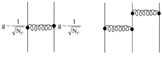
Figure 5: The strong coupling $\alpha_{S}(Q^{2})=g^{2}(Q^{2})/(4\pi)={12\pi}\,[(11N_{c}-2N_{f})\ln(Q^{2}/\Lambda^{2})]^{-1}\sim 1/N_{c}$ is inversely proportional to the number of colors $N_{c}$. Multigluon exchange diagrams involve higher powers of $g\sim 1/\sqrt{N_{c}}$. Therefore, two-quark operators are typically suppressed by $1/N_{c}$ and three-quark operators by $1/N_{c}^{2}$ compared to one-quark operators.

For example the relation between the neutron charge radius $r_{n}^{2}$ and $N\to\Delta$ transition quadrupole moment $Q_{N\to\Delta}$ in Eq.(1) has been investigated using the $1/N_{c}$ expansion method Hes02 . Including second and third order SU(6) symmetry breaking operators the following expression has been found:

$$Q_{N\to\Delta}=\frac{1}{\sqrt{2}}\,r_{n}^{2}\,\,\left(\frac{N_{c}}{N_{c}+3}\,\sqrt{\frac{N_{c}+5}{N_{c}-1}}\right).$$ (21)

It is interesting that this more general relation is equivalent to Eq.(1) both for the physical $N_{c}=3$ case and for $N_{c}\to\infty$. For arbitrary $N_{c}$, the difference between Eq.(21) and Eq.(1) is always less than 1.2$\%$.

Up to now we have discussed the application of three different SU(6) symmetry based methods to the ${\bf 56}$ dimensional representation of ground state baryons for which $J=S$ and $L=0$. When the orbital angular momentum $L$ of the states and operators is nonzero as for the $N^{*}(1680)$ resonance, the symmetry group has to be enlarged to SU(6)$\times$O(3). This was done in the case of the $1/N_{c}$ expansion by several authors Goi07 ; Coh05 ; Mat16 . In this work we use a fourth group theoretical method, namely current algebra. In sect. III.4 we employ current algebra to calculate transition multipole moments of excited states with $L\neq 0$. Current algebra stresses the importance of the commutation relations between group generators and explores the consequences that follow from this symmetry requirement.

III.4 Algebra of vector and axial vector current components

The algebra of electromagnetic and weak currents provides a group theoretical description of the structure of hadrons based on the concept that the vector and axial vector currents are proportional to group generators. Clearly, the electromagnetic currents involve the SU(3) generators $T_{3}=\lambda_{3}/2$ (isovector current $J^{3}$) and $Y=\lambda_{8}/\sqrt{3}$ (isoscalar current $J^{8}$) occuring in the Gell-Mann-Nishijima relation of Eq.(17) for the electric charge ${\rm{Q}}$. To describe weak vector currents, the isovector $T_{3}$ term of the electromagnetic current in Eq.(17) is generalized to strangeness conserving weak isovector-vector currents based on $T_{\pm}=(\lambda_{1}\pm i\lambda_{2})/2$, in addition to strangeness changing weak vector currents involving $V_{\pm}=(\lambda_{4}\pm i\lambda_{5})/2$ and $U_{\pm}=(\lambda_{6}\pm i\lambda_{7})/2$. The space integrals of these 8 vector currents $J^{\gamma}$ with $\gamma=1,...,8$ obey the same SU(3) commutation relations (Lie algebra) as the SU(3) generators Gel64 ,

$$\left[\lambda_{\alpha},\lambda_{\beta}\right]=2if_{\alpha\beta\gamma}\lambda_{\gamma},$$ (22)

where the $f_{\alpha\beta\gamma}$ are the antisymmetric SU(3)_F structure constants.

An analogous SU(3)_A algebra describes weak axial currents $J^{5\gamma}$. Thus, in electroweak theory one is dealing with a SU(3)${}_{V}\times$SU(3)_A group. When taking the linear combinations

$$J^{\gamma\pm}=J^{\gamma}\pm J^{5\,\gamma},$$ (23)

the new generators $J^{\gamma\pm}$ satisfy a closed system of commutation relations Gel64 . As emphasized by Gell-Mann, no matter how badly SU(3) flavor symmetry is broken, the group generators satisfy the algebraic commutation relations exactly. This observation is the basis of several important sum rules, such as the Adler-Weisberger sum rule relating the weak axial coupling to pion-nucleon scattering cross sections deA73 .

A further generalization based on the relativistic vector and axial-vector quark flavor currents involves the Dirac matrices $\gamma_{\mu}$ with $\mu=0,...3$ and $\gamma_{5}$

$$J_{\mu}^{\alpha}=\bar{q}\,\frac{1}{2}\lambda_{\alpha}\,\gamma_{\mu}\,q\ \ \ J_{\mu}^{5,\alpha}=\bar{q}\,\frac{1}{2}\,\lambda_{\alpha}\,\gamma_{\mu}\gamma_{5}\,q,$$ (24)

where $\alpha=0,...,8$ and $\lambda_{0}=\sqrt{2/3}\,\,{\bf 1}$. This leads to an algebra of $72=8\cdot 4\cdot 2$ vector and axial current components corresponding to the generators of a chiral U(6)${}_{V}\times$U(6)_A algebra. In the following, we use this generalized form of Gell-Mann’s current algebra Fey64 in which the time and spatial components of the vector current densities satisfy the following commutation relations Das65 ; Lee65 ; Bie66

$$\left[J_{0}^{\alpha}({\bf r}),\,J_{0}^{\beta}({\bf r}^{\prime})\right] = i\,f_{\alpha\beta\gamma}\delta({\bf r}-{\bf r}^{\prime})\,J_{0}^{\gamma}({\bf r}),$$

$$\left[J_{i}^{\alpha}({\bf r}),\,J_{j}^{\beta}({\bf r}^{\prime})\right] = i\,f_{\alpha\beta\gamma}\delta_{ij}\delta({\bf r}-{\bf r}^{\prime})\,J_{0}^{\gamma}({\bf r})$$ (25)

$$+ id_{\alpha\beta\gamma^{\prime}}\epsilon_{ijk}\delta({\bf r}-{\bf r}^{\prime})\,A_{k}^{\gamma^{\prime}}({\bf r}).$$

The flavor components of the spatial current $J_{i}^{\alpha}$ and charge $J_{0}^{\alpha}$ densities are denoted by greek superscripts $\alpha,\beta,\gamma$. The roman subscripts $i,j,k$ indicate the cartesian components of the spatial vector ${\bf J}$ and axial vector ${\bf A}={\bf J}^{5}$ currents. As usual, $\delta_{ij}$ and $\epsilon_{ijk}$ refer to the Kronecker and Levi-Civita tensors, and the $d_{\alpha\beta\gamma}$ are the symmetric SU(3) structure constants.

An early application of the current algebra method to magnetic moments led to the Gell-Mann Dashen relation between the proton magnetic moment $\mu_{p}$ and the proton charge radius $r_{p}$ Das65

$$\mu_{p}^{2}=\frac{1}{6}r_{p}^{2},$$ (26)

where $\mu_{p}$ is expressed in nuclear magnetons $\mu_{N}=1/(2M_{N})$ in units [fm]. Eq.(26) is satisfied within 20$\%$. In our application to quadrupole and octupole transition multipole moments we will also take space integrals of these charge current components similar to the work of Bietti Bie66 .

IV Results

IV.1 Charge radii of ground state baryons

As in Eq.(3) we expand the baryon charge density operator $\rho({\bf q})$ into Coulomb multipoles with projection $M=0$ up to quadrupole terms

$$\rho(q) \!\!\!=\!\!\! \sqrt{4\pi}\sum_{J}i^{J}{\hat{J}}T_{0}^{CJ}(q)\!\!=\!\!\rho^{C0}(q)+\rho^{C2}(q)+...,$$ (27)

which have been evaluated for $\hat{{\bf q}}={\bf e}_{z}$ so that $Y^{J}_{0}({\hat{\bf q}})={\hat{J}}/\sqrt{4\pi}$ with ${\hat{J}}=\sqrt{2J+1}$. The lowest moments of $\rho$ are then obtained from a low momentum transfer expansion of $j_{J}(gr)$ in Eq.(4). Up to $q^{2}$ contributions one has

$$\rho(q)={\rm Q}-\frac{q^{2}}{6}r^{2}-\frac{q^{2}}{6}{\mathcal{Q}}+...$$ (28)

The first two terms arise from the spherically symmetric monopole $\rho^{C0}$ part and the third term comes from the quadrupole $\rho^{C2}$ part of $\rho$. The low $q$ expansion of $\rho$ gives the baryon’s total charge (${\rm Q}$), spatial extension ($r^{2}$), and shape (${\mathcal{Q}}$).

According to the group theoretical approach outlined in sect. III.1 and sect. III.2, the charge radius is a rank $J=0$ operator and must be constructed as a sum of one-, two-, and three-quark terms, each of which transforming as an ${\bf(8,1)}$ representation in flavor-spin space, i.e. as a flavor octet and a spin scalar

$${r}^{2}=A\sum_{i=1}^{3}e_{i}{\bf 1}+B\sum_{i\neq j}^{3}e_{i}\,\mbox{\boldmath$\sigma$}_{i}\cdot\mbox{\boldmath$\sigma$}_{j}+C\!\!\sum_{i\neq j\neq k}^{3}e_{k}\,\mbox{\boldmath$\sigma$}_{i}\cdot\mbox{\boldmath$\sigma$}_{j},$$ (29)

where $e_{i}=(1+3\tau_{i\,z})/6$ and $\mbox{\boldmath$\sigma$}_{i}$ are the charge and spin operators of the i-th quark. Here, $\tau_{i\,z}$ denotes the $z$ component of the Pauli isospin matrix. These are the only allowed spin scalars and flavor octets that can be constructed from the generators of the spin-flavor group in Eq.(11). The constants $A$, $B$, and $C$ parametrizing the orbital and color matrix elements are determined from experiment.

Nucleon and $\Delta$ charge radii are then calculated by evaluating matrix elements of the operator in Eq.(29) between three-quark spin-flavor wave functions $|W_{B}\rangle$

$$r_{B}^{2}=\langle W_{B}|{r}^{2}|W_{B}\rangle.$$ (30)

For charged baryons, $r^{2}_{B}$ is normalized by dividing by the baryon charge. The results for octet and decuplet baryons are summarized in Table 2. A complete table including all 18 ground state baryon charge radii and the relations between them is given in Ref. Buc07 . The results agree with those in Ref. Leb00 after setting $N_{c}=3$ and an obvious redefinition of the constants.

Table 2: Nucleon and $\Delta$ charge radii in [fm²] with one-quark $(A)$, two-quark ($B$), and three-quark ($C$) contributions. Left: Analytic expressions for $r^{2}_{B}$ obtained from Eq.(30). Right: Numerical values using $r_{p}=0.8751(61)$ fm Pat16 , $r^{2}_{n}=-0.1149(35)$ fm² Kop97 , $r^{2}_{{\Sigma}^{-}}=0.61(12)$ fm² Esc01 as input yielding $A=0.7299$, $B=0.0455$, and $C=-0.0060$ in [fm²]. For details see Ref. Buc07 .

	$\ \ \ \ \ \ r_{B}^{2}$	$r_{B}^{2}$ [fm2]
$n$	$\phantom{A}-2B+4C$	-0.115
$p$	$A\phantom{\,\,2B+}-6C$	0.766
$\Delta^{-}$	$A+2B+2C$	0.809
$\Delta^{0}$	$\phantom{+++++}0$	0.809
$\Delta^{+}$	$A+2B+2C$	0.809
$\Delta^{++}$	$A+2B+2C$	0.809

IV.2 Quadrupole moments of ground state baryons

As explained in sect. III the charge quadrupole operator is constructed from flavor ${\bf 8}$ and spin $J=2$ operators as a sum of two- and three-body quark terms each transforming as an ${\bf(8,5)}$ representation in flavor-spin space

$$\mathcal{Q} = B^{\prime}\sum_{i\neq j}^{3}e_{i}\left(3\sigma_{i\,z}\sigma_{j\,z}-\mbox{\boldmath$\sigma$}_{i}\cdot\mbox{\boldmath$\sigma$}_{j}\right)$$ (31)

$$+ C^{\prime}\!\!\sum_{i\neq j\neq k}^{3}e_{k}\left(3\sigma_{i\,z}\sigma_{j\,z}-\mbox{\boldmath$\sigma$}_{i}\cdot\mbox{\boldmath$\sigma$}_{j}\right).$$

Baryon decuplet quadrupole moments $Q_{B^{*}}$ and octet-decuplet transition quadrupole moments $Q_{B\to B^{*}}$ are obtained by calculating the matrix elements of the quadrupole operator in Eq.(31) between the three-quark spin-flavor wave functions $|W_{B}\rangle$ and $|W_{B^{*}}\rangle$

$$Q_{B^{*}}\!\!=\!\!\left\langle W_{B^{*}}|\mathcal{Q}|W_{B^{*}}\right\rangle,\,\,Q_{B\to B^{*}}\!\!=\!\!\left\langle W_{B^{*}}|\mathcal{Q}|W_{B}\right\rangle,$$ (32)

where $B$ denotes a spin 1/2 octet baryon and $B^{*}$ a member of the spin 3/2 baryon decuplet. The ensuing results for quadrupole moments and the relations between them have been discussed earlier Hes02 ; Hen02 ; Leb00 . Table 3 reproduces some pertinent results.

Table 3: Transition and diagonal baryon quadrupole moments with two-quark (B’) and three-quark (C’) contributions Hen02 ; Buc07 . Left: Analytic expressions for $Q_{B}$ obtained from Eq.(32). Right: Numerical values using the parameter set of Table 2 with $B^{\prime}=-B/2$, $C^{\prime}=-C/2$, and $\zeta=m_{u}/m_{s}=0.613$. We then obtain $Q_{p\to\Delta^{+}}({\rm theory})=-0.0812(25)$ fm² with $r_{n}^{2}$ as input compared to $Q_{p\to\Delta^{+}}({\rm exptl})=-0.0846(33)$ fm² Tia11 and $Q_{p\to\Delta^{+}}({\rm exptl})=-0.108(9)$ fm² Bla01 .

	$\ \ \ \ Q_{B}$	$Q_{B}$ [fm2]
$n\to\Delta^{0}$	$2\sqrt{2}(B^{\prime}-2C^{\prime})$	-0.081
$p\to\Delta^{+}$	$2\sqrt{2}(B^{\prime}-2C^{\prime})$	-0.081
$\Delta^{-}$	$-4B^{\prime}-4C^{\prime}$	0.079
$\Delta^{0}$	0	0
$\Delta^{+}$	$4B^{\prime}+4C^{\prime}$	-0.079
$\Delta^{++}$	$8B^{\prime}+8C^{\prime}$	-0.158
$\Omega^{-}$	$-(4B^{\prime}+4C^{\prime})\zeta^{3}$	0.018

In this work, we are mainly concerned with relations between the measureable transition quadrupole moments and nucleon ground state properties. To this end, we will first show that $B^{\prime}=-B/2$. One can understand the result $B^{\prime}=-B/2$ from the explicit expression Buc91 for the one-gluon exchange charge density in Fig. 4

$$\rho_{gq{\bar{q}}} = -i\frac{\alpha_{S}}{16m_{q}^{3}}\sum_{i<j}^{3}\mbox{\boldmath$\lambda$}_{i}\cdot\mbox{\boldmath$\lambda$}_{j}\bigl{(}e_{i}e^{i{\bf q}\cdot{\bf r}_{i}}(\mbox{\boldmath$\sigma$}_{i}\times{\bf q})\cdot(\mbox{\boldmath$\sigma$}_{j}\times{\bf r})$$ (33)

$$+ (i\leftrightarrow j)\bigr{)}\frac{1}{r^{3}},$$

where $\mbox{\boldmath$\lambda$}_{i}$ are the SU(3) color matrices of quark i. Here we have reproduced only the spin-dependent terms of $\rho_{gq{\bar{q}}}$ that contribute to $r_{n}^{2}$ and $Q_{p\to\Delta^{+}}$.

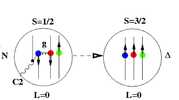
Figure 6: The $q{\bar{q}}$-gluon exchange charge density $\rho_{[2]}$ in Fig. 4 induces the $N\to\Delta$ charge quadrupole (C2) transition via a double spin-flip of two quarks, i.e. via the spin tensor term in Eq.(34). Siegert’s theorem connects this double spin-flip process with a spatial exchange current providing the dominant contribution to the $N\to\Delta$ transverse electric (E2) form factor Buc98 .

After some angular momentum recoupling we can rewrite Eq.(33) as a superposition of a spin scalar and a spin tensor term depicted in Fig. 6 with definite relative weight as

$$\rho_{gq\overline{q}}=B\sum_{i\neq j}^{3}e_{i}\left[\,(-2)\,\mbox{\boldmath$\sigma$}_{i}\cdot\mbox{\boldmath$\sigma$}_{j}+(3\sigma_{i\,z}\sigma_{j\,z}-\mbox{\boldmath$\sigma$}_{i}\cdot\mbox{\boldmath$\sigma$}_{j})\right].$$ (34)

The factor $B$ contains the radial, momentum, and color dependence common to both spin-dependent terms. Thus, for the gluon exchange charge density shown in Fig. 4 there is a fixed ratio of (-2) between the spin scalar and spin tensor parts of the corresponding operator. The same relative factor is obtained for pion exchange or a combination of gluon and pion exchange between quarks. The relative factor (-2) between spin scalar and spin tensor turns out to be a model-independent symmetry based property of two-quark charge densities.

If the fixed ratio between spin scalar and spin tensor is implemented in the GP method, relation Eq.(1) follows from the expressions in Table 2 and Table 3 as

$$Q_{p\to\Delta^{+}}=2\sqrt{2}(B^{\prime}-2C^{\prime})=-\sqrt{2}(B-2C)=\frac{1}{\sqrt{2}}\,r_{n}^{2}.$$ (35)

In appendix A, we provide a group theoretical derivation of this fixed ratio and of Eq.(1) based on broken spin-flavor symmetry without making any dynamical assumptions.

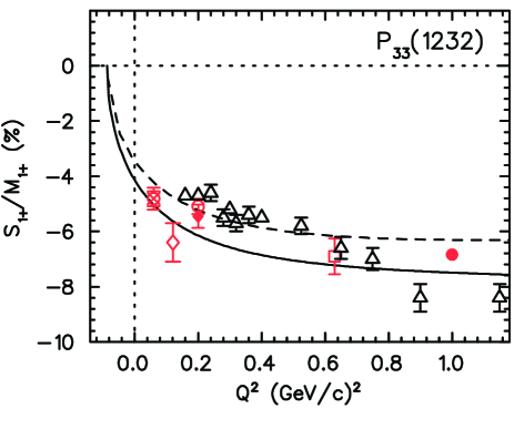
Figure 7: The $C2/M1(Q^{2})\equiv S_{1+}/M_{1+}(Q^{2})$ ratio for low four-momentum transfers. The full curve is a fit of the experimental $C2/M1$ ratio as determined from the world electro-pionproduction data. The dashed curve is calculated using the form factor relation of Eq.(2). Figure taken from Ref. tia16 .

From the form factor relation in Eq.(2) we can also extract the quadrupole transition radius, which is determined by the fourth and second radial moments of the neutron charge distribution Buc09

$$r^{2}_{C2}=\frac{7}{10}\,\frac{r^{4}_{n}}{r^{2}_{n}}.$$ (36)

From the radial moments of the neutron charge density in Table 5 we find $r_{C2}=1.68\,{\rm fm}$. Thus, $r_{C2}\approx r_{\pi}$ is close to the pion Compton wavelength. We have previously suggested that $r_{C2}$ measures the spatial extension of the $q{\bar{q}}$ pair distribution in the nucleon Buc09 . Recently, $r_{C2}$ has been determined from combined fits of the $G_{C}^{n}$ and $G_{C2}^{N\to\Delta}$ form factor data Ram17 obtaining a somewhat smaller value $r_{C2}=1.32$ fm.

Broken SU(6) spin-flavor symmetry also leads to the following relation Beg64 between the neutron elastic and the $N\to\Delta$ transition magnetic form factors, and at $Q^{2}=0$ between the neutron and $N\to\Delta$ transition magnetic moments

$$G_{M1}^{N\to\Delta}(Q^{2})=-\sqrt{2}\,G_{M}^{n}(Q^{2}),\quad\mu_{N\to\Delta}=-\sqrt{2}\,\mu_{n}.$$ (37)

With the help of Eq.(2) and the magnetic form factor relation of Eq.(37), the C2/M1 ratio in electromagnetic $\Delta(1232)$ excitation can be expressed in terms of the neutron elastic form factors as follows Buc04

$$\frac{C2}{M1}(Q^{2}) := \frac{|{\bf q}|\,M_{N}}{6}\,\frac{G_{C2}^{N\to\Delta}(Q^{2})}{G_{M1}^{N\to\Delta}(Q^{2})}=\frac{|{\bf q}|M_{N}}{2\,Q^{2}}\,\frac{G_{C}^{n}(Q^{2})}{G_{M}^{n}(Q^{2})},$$

$$\frac{C2}{M1}(0) = -\frac{(M_{\Delta}^{2}-M_{N}^{2})}{2M_{\Delta}}\,\frac{M_{N}}{12}\frac{r_{n}^{2}}{\mu_{n}}.$$ (38)

where $|{\bf q}|$ is the modulus of the photon’s three-momentum and $M_{N}$, $M_{\Delta}$ are the nucleon and $\Delta$ masses. The dashed curve in Fig. 7 shows that the prediction based on Eq.(IV.2) agrees quite well with the data. Moreover, it has the correct limiting behavior for $Q^{2}\to 0$ and $Q^{2}\to\infty$ Idi04 ; tia16 . In particular, for $Q^{2}=0$ we get $C2/M1=-3.1\%$ in good agreement with recent experimental results Blo16 .

The electromagnetic $N\to\Delta$ transition multipoles also affect other observables. It has recently been shown Hag18 that the $\Delta$(1232) resonance has an appreciable impact on the spectrum of atomic hydrogen.

IV.3 Intrinsic charge quadrupole form factor of the nucleon

To study the implications of Eq.(1) and Eq.(2) for the shape of the nucleon ground state it is important to distinguish between the spectroscopic and intrinsic quadrupole moment of a particle Boh75 . It is known that a vanishing spectroscopic quadrupole moment due to angular momentum selection rules does not necessarily imply a spherically symmetric charge distribution. For deformed spin 0 and spin 1/2 nuclei this insight has led to the general concept of an intrinsic quadrupole moment, which can be defined for different nuclear models. The notion of an intrinsic quadrupole moment allows us to interpret measurable transition quadrupole moments in terms of the shape of the ground state.

The geometric shape of a spatially extended particle is determined by its intrinsic quadrupole moment,

$$Q_{0}=\int\!\!d^{3}r\,\rho({\bf r})\,(3z^{2}-r^{2}),$$ (39)

which is defined with respect to the body-fixed frame. If the charge density is concentrated along the $z$-direction (symmetry axis of the particle), the term proportional to $3z^{2}$ dominates, $Q_{0}$ is positive, and the particle is prolate (cigar-shaped). If the charge density is concentrated in the equatorial plane perpendicular to $z$, the term proportional to $r^{2}$ prevails, $Q_{0}$ is negative, and the particle is oblate (pancake-shaped) as depicted in Fig. 8.

Figure 8: Prolate (left) and oblate (right) charge distribution corresponding to a positive (negative) intrinsic quadrupole moment $Q_{0}$ defined as in Eq.(39). An analogous figure is obtained for the current distribution with $Q_{0}$ replaced by $\Omega_{0}$.

Previously, we have found for the intrinsic quadrupole moment of the proton and $\Delta^{+}$ in the quark model with two-body exchange currents Hen01

$$Q_{0}^{p}=-r^{2}_{n},\qquad Q_{0}^{\Delta^{+}}=r^{2}_{n}.$$ (40)

Thus, the intrinsic quadrupole moment of the proton is given by the negative of the neutron charge radius and is therefore positive, whereas the intrinsic quadrupole moment of the $\Delta^{+}$ is negative. This corresponds to a prolate proton and an oblate $\Delta^{+}$ shape. The quark model with exchange currents also suggests that the nonsphericity of the proton charge density is mainly connected with collective quark-antiquark degrees of freedom, the distribution of which has a prolate shape.

The concept of an intrinsic quadrupole moment of the nucleon can be generalized to an intrinsic quadrupole charge distribution and a corresponding form factor buc05 ; Buc07b . To show this, we first decompose the proton and neutron charge form factors in two terms $G_{C,sym}$ and $G_{C,def}$, coming from the spherically symmetric and the intrinsic quadrupole part of the physical charge density respectively

$$G_{C}^{p}(Q^{2})\! = \!G_{C,sym}^{p}(Q^{2})-\frac{1}{6}\,Q^{2}\,G_{C,def}(Q^{2}),$$

$$G_{C}^{n}(Q^{2})\! = \!G_{C,sym}^{n}(Q^{2})+\frac{1}{6}\,Q^{2}\,G_{C,def}(Q^{2}).$$ (41)

The factor $Q^{2}$ in front of $G_{C,def}$ arises for dimensional reasons and guarantees that the normalization of the charge form factors is preserved.

In coordinate space this corresponds to the usual multipole decomposition of the charge density

$$\rho({\bf r})=\underbrace{\rho_{0}(r)Y^{0}_{0}({\bf r})}_{{\rm monopole}}+\underbrace{\rho_{2}(r)Y^{2}_{0}({\bf r})}_{{\rm quadrupole}}+\ldots,$$ (42)

where the $\rho_{0}(r)$ part gives rise to $G_{C,sym}(Q^{2})$ and the $\rho_{2}(r)$ part is connected with $G_{C,def}(Q^{2})$. In terms of fundamental photon-quark processes depicted in Fig. 4 the monopole part $G_{C,sym}$ comes from one-quark currents, whereas the intrinsic quadrupole part $G_{C,def}$ is mainly due to two- and three-quark currents.

From the relation between the measurable $N\to\Delta$ quadrupole and elastic neutron charge form factors in Eq.(2) we find for the intrinsic charge quadrupole form factor $G_{C,def}(Q^{2})$ of the nucleon

$$G_{C,def}(Q^{2}) = -\sqrt{2}G_{C2}^{N\to\Delta}(Q^{2})=\frac{6}{Q^{2}}G_{C}^{n}(Q^{2}),$$

$$G_{C,def}(0) = -r_{n}^{2}=Q_{0}^{p}.$$ (43)

The zero momentum limit follows from l’ Hospital’s rule and Eq.(40). This shows that $G_{C,def}(Q^{2})$ as defined in Eq.(IV.3) is the proper generalization of the intrinsic quadrupole moment $Q_{0}^{p}$ to finite momentum transfers.

To exhibit the effect of the intrinsic quadrupole form factor on the elastic nucleon form factors we insert Eq.(IV.3) into Eq.(IV.3) and obtain

$$G_{C}^{p}(Q^{2}) = G_{C,sym}^{p}(Q^{2})-G_{C}^{n}(Q^{2})$$

$$= \underbrace{G_{C}^{IS}(Q^{2})}_{{\rm spherical}}-\underbrace{G_{C}^{n}(Q^{2})}_{{\rm deformed}},$$

$$G_{C}^{n}(Q^{2}) = \frac{1}{6}\,Q^{2}\,G_{C,def}(Q^{2}),$$ (44)

where the isoscalar nucleon charge form factor is defined as

$$G_{C}^{IS}(Q^{2})=G_{C}^{p}(Q^{2})+G_{C}^{n}(Q^{2}).$$ (45)

We propose that $G_{C,sym}^{n}(Q^{2})=0$ so that the neutron charge form factor is solely given by $G_{C,def}(Q^{2})$ as stated in Eq.(IV.3). Thus, the relation between the $N\to\Delta$ and neutron charge form factors in Eq.(2) is seen here to have an important implication for the nucleon ground state itself.

There are several observable consequences of Eq.(IV.3) and Eq.(IV.3) as discussed in Ref. buc05 ; Buc07b . At low $Q^{2}$ the nucleon’s prolate deformation is reflected in a proton charge radius increase by an amount $-r_{n}^{2}$, with respect to $r_{IS}^{2}$ and by a novel nucleon size parameter $r_{def}^{2}=r^{2}_{C2}=(7/10)(r_{n}^{4}/r_{n}^{2})$ measuring the extension of the intrinsic quadrupole charge density. At intermediate $Q^{2}$ it leads to the conclusion that the dip structure observed in the proton charge form factor fri03 at around $Q^{2}\approx 0.3$ GeV² is due to a corresponding structure in the neutron charge form factor at the same $Q^{2}$. Finally, at high $Q^{2}$ it leads to the observed decrease of the charge over magnetic form factor ratio jon00 .

IV.4 $N\to N^{*}(1680)$ transition quadrupole moment

After projecting the charge-charge commutation relation in Eq.(III.4) onto the Coulomb quadrupole part by multiplying with $\sqrt{16\pi/5}\,r^{2}\,Y^{2}_{0}(\hat{{\bf r}})$ and integrating over space we get

$$\left[Q_{z}^{\alpha},Q_{z}^{\beta}\right]=if_{\alpha\beta\gamma}\,\int\,d^{3}{\bf r}(3z^{2}-r^{2})^{2}\,\rho^{\gamma}({\bf r}),$$ (46)

where

$$Q_{z}^{\alpha}=\int\,d^{3}{\bf r}(3z^{2}-r^{2})\,\rho^{\alpha}({\bf r}).$$ (47)

For the flavor (isospin) index we take $\alpha=1$ and $\beta=2$, entailing $\gamma=3$ and $f_{123}=1$. The subscript indicates the $z$ component of the quadrupole tensor. For calculational convenience we transform in flavor (isospin) space from a cartesian to a spherical basis using the ladder operators

$$Q^{\pm}=\mp\frac{1}{\sqrt{2}}\,(Q^{1}\pm i\,Q^{2}),\ \ \ \ Q^{0}=Q^{3}.$$ (48)

which leads to

$$\left[Q_{z}^{+},Q_{z}^{-}\right]=-\int\,d^{3}{\bf r}\,(3z^{2}-r^{2})^{2}\rho^{0}({\bf r}).$$ (49)

Table 4: Empirical helicity amplitudes $A_{1/2}$, $A_{3/2}$ and $S_{1/2}$ in units $[10^{-3}$ GeV${}^{-1/2}]$ tia16 ; Tia11 ; Pat16 for the electromagnetic $N\to N^{*}(1680)$ transition and the corresponding quadrupole moment $Q_{N\to N^{*}(1680)}$ in units [fm²] determined from the transverse helicity amplitudes and Siegert’s theorem (5th column) or directly from the scalar helicity amplitude $S_{1/2}$ (last column).

	$A_{1/2}$	$A_{3/2}$	$S_{1/2}$	$Q_{N\to N^{*}}$	$Q_{N\to N^{*}}$
$p\to p^{*}$	$-15\pm 6$	$\phantom{-}133\pm 12$	$-44$	0.203(27)	0.073
$n\to n^{*}$	$\phantom{-}29\pm 10$	$-33\pm 9$	$0$	$-0.021(27)$	$0$

For an evaluation between nucleon ground states with orbital angular momentum $L=0$, the right-hand side can be simplified as follows

$$\langle p|\left[Q_{z}^{+},Q_{z}^{-}\right]|p\rangle=-\frac{4}{5}\langle p|\int\,d^{3}{\bf r}\,r^{4}\rho^{0}({\bf r})|p\rangle.$$ (50)

Note that the right hand side is nonzero even though the proton does not have a spectrosopic quadrupole moment. Inserting on the left-hand side a sum of intermediate $N^{*}$ resonances

$$\sum_{N^{*}}|N^{*}\rangle\langle N^{*}|=1$$ (51)

of which only those contribute that can be reached with an orbital angular momentum $L=2$ and an isospin $T=1$ operator such as $Q^{\pm}$ we obtain a relation between the fourth moment of the ground state charge density and a sum of squared transition quadrupole moments.

If we include only the $N^{*}(1680)$ as intermediate state, we get

$$\langle p|Q_{z}^{+}|n^{*}(1680)\rangle\,\langle n^{*}(1680)|Q_{z}^{-}|p\rangle$$ (52)

$$= -2Q^{2}_{IV}(p\to p^{*}(1680))=-\frac{4}{5}\,r_{IV}^{4}(p),$$

where we have converted $Q_{z}^{\pm}$ back to $Q_{z}^{0}$ using the Wigner-Eckart theorem in isospin space. Here, $Q_{IV}(p\to p^{*}(1680))$ and $r_{IV}^{4}(p)$ denote the isovector parts of the proton’s transition quadrupole moment and fourth radial moment This leads to the result

$$Q_{IV}(p\to p^{*}(1680))=\sqrt{\frac{1}{5}(r_{p}^{4}-r_{n}^{4})},$$ (53)

where $r_{p}^{4}$ ($r_{n}^{4}$) is the fourth radial moment of the proton (neutron) charge distribution. This agrees with Bietti Bie66 except for a factor 2 on the right-hand side not contained in Ref. Bie66 .

For numerical evaluation we need the nucleon structure parameters $r_{p}^{4}$ and $r_{n}^{4}$, which are connected with the curvature of the corresponding charge monopole form factors. These are not very well known experimentally. For example, for the fourth radial moment the following values can be found in the literature: $r_{p}^{4}=0.82\pm 1.02$ fm⁴ Gri16 , $r_{p}^{4}=1.32\pm 0.96$ fm⁴ Hig16 , $r_{p}^{4}=2.01\pm 0.05$ fm⁴ Sic17 , $r_{p}^{4}=2.59\pm 0.19$ fm⁴ Dis11 .

We have calculated the lowest radial moments of the proton and neutron using the form factor decomposition in Eq.(IV.3), where we have used the Galster Gal71 parametrization for the neutron charge form factor, and a dipole form for the isoscalar nucleon form factor

$$G_{C}^{n}(Q^{2}) = -\frac{a\tau}{1+d\tau}\,\frac{\mu_{n}}{(1+Q^{2}/\Lambda^{2}_{M})^{2}}$$

$$G_{C}^{IS}(Q^{2}) = (1+Q^{2}/\Lambda^{2}_{IS})^{-2}.$$ (54)

This leads to the radial moments listed in Table 5.

Table 5: Radial moments of the proton and neutron charge distribution based on the form factor decomposition of Eq.(IV.3) using the following parameters: $\Lambda^{2}_{M}=19.87$ fm^-2 determined from the experimental proton magnetic radius $r_{M}=0.777$ fm² Ber10 $\Lambda^{2}_{IS}=18.43$ fm^-2 determined from the experimental isoscalar radius $r^{2}_{IS}=0.651$ fm² and $a=0.9$, $d=1.75$ from a fit to the neutron form factor data Gra01 .

	$r^{2}$ [fm2]	$r^{4}$ [fm4]	$r^{6}$ [fm6]
$p$	$0.7658$	$1.3356$	$4.4070$
$n$	$-0.1149$	$-0.2757$	$-1.1866$

Using the empirical helicity amplitudes from PDG Pat16 and MAID tia16 ; Tia11 listed in Table 4 and the conversion formulae given in Appendix B we obtain for the experimental $N\to N^{*}(1680)$ transition quadrupole moments

$$Q_{p\to p^{*}(1680)} = 0.203(27)\,{\rm fm}^{2}$$

$$Q_{n\to n^{*}(1680)} = -0.021(27)\,{\rm fm}^{2}$$ (55)

based on the transverse helicity amplitudes and Siegert’s theorem. This gives $Q_{IV}(p\to p^{*}(1680))=0.112(27)$ fm²(exptl). Alternatively, from the scalar helicity amplitudes we get $Q_{IV}(p\to p^{*}(1680))=0.037$ fm²(exptl). This has to be compared to $Q_{IV}(p\to p^{*}(1680))=0.57$ fm²(theory) from Eq.(53), where we have used $r_{p}^{4}=1.34$ fm⁴ and neutron $r_{n}^{4}=-0.28$ fm⁴ from Table 5.

Evidently, the agreement between a theory based on a single intermediate resonance and experiment is fairly bad. But the nucleon spectrum has several more resonances Cre13 ; Bur15 with quantum numbers that can be reached by an $L=2$ operator, e.g. the positive parity states $p^{*}(1860)$ and $p^{*}(2000)$ with $J=5/2$ in addition to the $p^{*}(1720)$ and $p^{*}(1900)$ resonance with $J=3/2$. Including these excited states on the commutator side, we obtain $Q_{IV}(p\to p^{*})\approx 0.25$ fm²(theory). If additional excited states exist, the agreement between theory and experiment may further improve. Aside from the uncertainty related to the number of excited states, there is considerable uncertainty with respect to the fourth radial moments of the ground state charge distribution, which are not well known experimentally.

Clearly, more detailed theories achieving better agreement with experiment may be formulated. In this work, our main point is to study the relationship between transition multipole moments and ground state properties. The present symmetry based current algebra approach makes this connection to some extent transparent. In particular, our results suggest that the radial moments $r_{p}^{4}$ and $r_{n}^{4}$ are connected with the quadrupole excitation of the $p^{*}(1680)$ resonance.

IV.5 Magnetic octupole moments of ground state baryons

For the construction of a rank $J=3$ magnetic octupole moment operator from the generators of the group SU(6) group we need a tensor of rank 3 in spin space. This operator must involve the Pauli spin matrices of three different quarks. If two of these had the same particle index, the SU(2) spin commutation relations would reduce their action to a single Pauli matrix, and we could only build a spin tensor of rank 2. Therefore, a tensor of rank 3 in spin space must necessarily be a three-quark operator.

We have previously shown that the magnetic octupole moment operator can be constructed from a two-body quadrupole moment operator multiplied by the spin of the third quark Buc08

$${\Omega}_{[3]} = C\sum_{i\neq j\neq k}^{3}e_{i}\left(3\sigma_{i\,z}\sigma_{j\,z}-\mbox{\boldmath$\sigma$}_{i}\cdot\mbox{\boldmath$\sigma$}_{j}\right)\mbox{\boldmath$\sigma$}_{k}.$$ (56)

As a three-body operator $\Omega$ transforms according to the 2695 irrep of SU(6), which occurs only once on the right-hand side of Eq.(13). In addition, Eq.(16) shows that the flavor 8, spin 3 tensor $({\bf 8},{\bf 7})$ appears only once in this decomposition. Hence, for the ${\bf 56}$ dimensional irrep of ground state baryons there is a unique three-quark magnetic octupole operator.

The magnetic octupole moments $\Omega_{B^{*}}$ are obtained by calculating the matrix elements of the octupole operator $\Omega_{[3]}$ between the three-quark spin-flavor wave functions $|W_{B^{*}}\rangle$

$$\Omega_{B^{*}} = \left\langle W_{B^{*}}|{\Omega}_{[3]}|W_{B^{*}}\right\rangle,$$ (57)

where $B^{*}$ denotes a member of the spin 3/2 baryon decuplet. For example, sandwiching Eq.(56) between the spin-isospin wave functions of the $\Delta(1232)$ gives

$$\Omega_{\Delta} = \langle W_{\Delta}|{{\Omega}}_{[3]}|W_{\Delta}\rangle=4Ce_{\Delta},$$ (58)

where $e_{\Delta}$ is the $\Delta$ charge. Similarly, the magnetic octupole moments for the other decuplet baryons are calculated. In this way Morpurgo’s method yields an efficient parameterization of baryon octupole moments in terms of just one unknown parameter Buc08 .

To obtain an estimate for $\Omega_{\Delta^{+}}$ we use the pion cloud model Hen01 where the $\Delta^{+}$ wave function for maximal spin projection is written as

$$|\Delta^{+}J_{z}=\frac{3}{2}\rangle=\beta^{\prime}\Bigl{(}\sqrt{\frac{1}{3}}|n^{\prime}\pi^{+}\rangle+\sqrt{\frac{2}{3}}|p^{\prime}\pi^{0}\rangle\Bigr{)}|\uparrow Y^{1}_{1}(\hat{{\bf r}}_{\pi})\rangle.$$ (59)

In this model the magnetic octupole moment operator is a product of a quadrupole operator in pion variables and a magnetic moment operator in nucleon variables

$$\Omega_{\pi N}=\sqrt{\frac{16\pi}{5}}\,r_{\pi}^{2}\,Y^{2}_{0}(\hat{{\bf r}}_{\pi})\,\,\mu_{N}\,\tau_{z}^{N}\,\sigma_{z}^{N},$$ (60)

where $\mu_{N}=1/(2M_{N})$ is the nuclear magneton. Here, the spin-isospin structure of $\Omega_{\pi N}$ is infered from the $\gamma\pi N$ and $\gamma\pi$ currents of the static pion-nucleon model Hen62 .

With these expressions the $\Delta^{+}$ magnetic octupole moment is readily calculated Hen01

$$\Omega_{\Delta^{+}}=-\frac{2}{15}\,{\beta^{\prime}}^{2}\,r_{\pi}^{2}\ \mu_{N}=Q_{\Delta^{+}}\,\mu_{N}=r_{n}^{2}\,\mu_{N},$$ (61)

where $Q_{\Delta^{+}}$ is the $\Delta^{+}$ quadrupole moment and $r_{n}^{2}$ the neutron charge radius. With the experimental value of the latter and $\mu_{N}$ expressed in $[{\rm fm}]$ one gets $\Omega_{\Delta^{+}}=-0.012\,\,{\rm fm^{3}}$. The negative value of $\Omega_{\Delta^{+}}$ implies that the magnetic moment distribution in the $\Delta^{+}$ is oblate and hence has the same geometric shape as the charge distribution as shown in Fig. 8.

In Table 6 we show our results for the decuplet octupole moments of the $\Delta$ and the $\Omega^{-}$ baryon expressed in terms of the GP constant $C$. Results for other decuplet baryons can be found in Ref. Buc08 .

Table 6: Magnetic octupole moments of decuplet baryons with $C=-0.003$ fm³ as determined from Eq.(61) and Eq.(58). SU(3) flavor symmetry breaking is characterized by the ratio $r$ of u-quark and s-quark masses $r=m_{u}/m_{s}=0.6$. From Ref. Buc08 .

	$\Omega$	$\Omega$  [fm3]
$\Delta^{-}$	$-4C$	$0.012$
$\Delta^{0}$	$0$	0
$\Delta^{+}$	$4C$	$-0.012$
$\Delta^{++}$	$8C$	$-0.024$
$\Omega^{-}$	$-4C\,r^{3}$	$0.003$

IV.6 Intrinsic magnetic octupole form factor of the nucleon

It is now fairly certain that the nucleon ground state charge distribution is not spherically symmetric. The geometric shape of the nucleon charge distribution is described by its intrinsic quadrupole moment $Q_{0}$ as discussed in sect. IV.3. It is conceivable that also the spatial current distribution and specifically the magnetic moment distribution inside the nucleon deviates from spherical symmetry. The existence of a nonvanishing $\Delta$ magnetic octupole and a fairly large $p\to p^{*}(1680)$ magnetic octupole moment provide some evidence that the nucleon has an intrinsic magnetic octupole moment.

Note that the definition for the octupole moment in Eq.(II.2) is analogous to the one for the charge quadrupole moment if the magnetic moment density $({\bf r}\times{\bf J}({\bf r}))_{z}$ is replaced by the charge density $\rho({\bf r})$. Thus, the magnetic octupole moment measures the deviation of the spatial magnetic moment distribution from spherical symmetry. Specifically, for a prolate (cigar-shaped) magnetic moment distribution $\Omega>0$, while for an oblate (pancake-shaped) magnetic moment distribution $\Omega<0$ as depicted in Fig. 8. We also see from Eq.(II.2) that the typical size of a magnetic octupole moment is

$$\Omega\simeq\mu\,r^{2}$$ (62)

where $\mu$ is the magnetic moment and $r^{2}$ a size parameter related to the quadrupole moment of the system.

From Eq.(61) and the discussion in sect. IV.3 we infer

$$\Omega_{0}^{\Delta^{+}}=r_{n}^{2}\,\mu_{N},\qquad\Omega_{0}^{p}=-r_{n}^{2}\,\mu_{N}.$$ (63)

Eq.(61) is seen to be the zero-momentum transfer limit of the magnetic octupole form factor of the $\Delta^{+}$

$$G_{M3}^{\Delta^{+}}(Q^{2})=-\frac{6}{Q^{2}}\,G_{C}^{n}(Q^{2})\,\mu_{N}.$$ (64)

Analogous to the discussion in sect. IV.3 we decompose the magnetic dipole form factor of the proton in two terms $G_{M,sym}$ and $G_{M,def}$, coming from the spherically symmetric and the intrinsic octupole part of the magnetic moment density respectively

$$G_{M}^{p}(Q^{2})=G_{M,sym}^{p}(Q^{2})-\frac{1}{6}\,Q^{2}\,G_{M,def}(Q^{2}).$$ (65)

The factor $Q^{2}$ in front of $G_{M,def}$ arises for dimensional reasons and guarantees that the magnetic moment of the proton remains unchanged. For $G_{M,sym}^{p}(Q^{2})$ we take a dipole form factor $G_{M,sym}^{p}(Q^{2})=\mu_{p}[1+Q^{2}/\Lambda^{2}_{M}]^{-2}$. For the intrinsic magnetic octupole form factor $G_{M,def}(Q^{2})$ we find

$$G_{M,def}(Q^{2})=-G_{M3}^{\Delta^{+}}(Q^{2})=\frac{6}{Q^{2}}\,G_{C}^{n}(Q^{2})\,\mu_{N}$$ (66)

which gives $G_{M,def}(0)=\Omega_{0}^{p}=-r_{n}^{2}\mu_{N}$ and thus shows that $G_{M,def}(Q^{2})$ is the proper generalization of Eq.(63) to finite momentum transfers.

To exhibit the effect of the intrinsic octupole form factor on the magnetic dipole form factor of the nucleon we insert Eq.(66) into Eq.(65) and obtain

$$G_{M}^{p}(Q^{2}) = G_{M,sym}^{p}(Q^{2})-G_{C}^{n}(Q^{2})\mu_{N}.$$ (67)

At low $Q^{2}$ the proton’s prolate magnetic dipole distribution leads to a small magnetic radius increase by an amount $-r_{n}^{2}\,\mu_{N}/\mu_{p}$ relative to the symmetric part given by $12/\Lambda^{2}_{M}$. At intermediate $Q^{2}$ our finding suggests that the dip structure observed in the proton magnetic form factor fri03 at around $Q^{2}\approx 0.3$ GeV² is due to a corresponding structure in the neutron charge form factor at the same $Q^{2}$.

IV.7 $N\to N^{*}(1680)$ transition octupole moment

After projecting the current-current commutation relation in Eq.(III.4) onto the magnetic octupole parts of the currents according to Eq.(II.2) we obtain

$$\left[\tilde{\Omega}^{1}_{z},\tilde{\Omega}^{2}_{z}\right] = i\,\left(\frac{3}{8}\right)^{2}(2\,M_{N})^{2}$$ (68)

$$\int d^{3}r\,(3z^{2}-r^{2})^{2}\,(x^{2}+y^{2})\,\rho^{3}({\bf r}),$$

where $\rho^{3}({\bf r})$ is the isovector component of the charge density. The axial current term on the right hand side in Eq.(III.4) does not contribute here because by definition the magnetic octupole moment operators are evaluated for the $z$ component that is for $i=j=3$.

Converting to a spherical basis in isospin space analogous to Eq.(48) and sandwiching Eq.(68) between proton ground states we obtain

$$\langle p|\tilde{\Omega}^{+}_{z}|n^{*}(1680)\rangle\langle n^{*}(1680)|\tilde{\Omega}^{-}_{z}|p\rangle$$ (69)

$$= \frac{3}{56}\,\,(2\,M_{N})^{2}\,\,\langle p|\int d^{3}r\,\,r^{6}\,\rho^{0}({\bf r})\,|p\rangle$$

where we have included only the $n^{*}(1680)$ intermediate state with spin $5/2$ and isospin $1/2$. With the help of the Wigner-Eckart theorem the left-hand side can be expressed in terms of the isovector part of the $p\to p^{*}(1680)$ transition octupole moment. Eq.(69) then provides a relation between the isovector $p\to p^{*}(1680)$ transition octupole moment and the sixth moments of the proton and neutron charge distributions

$$\Omega_{IV}(p\to p^{*}(1680))=\sqrt{\frac{3}{224}\left(r^{6}_{p}-r^{6}_{n}\right)}.$$ (70)

A numerical estimate for $\Omega_{IV}(p\to p^{*}(1680))$ based on the radial moments in Table 5 gives $\Omega_{IV}(p\to p^{*}(1680))=0.27$ fm³(theory) for a single resonance. If the 2 additional excited $J=5/2$ states seen in the spectrum are included on the commutator side we get $\Omega_{IV}(p\to p^{*})\approx 0.16$ fm³(theory).

To compare our theory with experiment, we use the conversion formulae in Appendix B and the helicity amplitudes in Table 4 and get

$$\Omega_{p\to p^{*}(1680)} = 0.164(22)\,{\rm fm}^{3},$$

$$\Omega_{n\to n^{*}(1680)} = -0.079(25)\,{\rm fm}^{3}.$$ (71)

This gives for the isovector term of the proton transition octupole moment $\Omega_{IV}(p\to p^{*}(1680))=0.121(23)$ fm³(exptl) compared to $\Omega_{IV}(p\to p^{*}(1680))=0.27$ fm³(theory).

Finally, we calculate the $p\to p^{*}(1680)$ transition multipole ratio

$$\frac{C2}{M3}(Q^{2}=0):=\frac{15}{4|{\bf q}|}\,\frac{Q_{p\to p*(1680)}}{\Omega_{p\to p^{*}(1680)}},$$ (72)

which gives for the isovector part of the $N\to N^{*}$ transition $(C2/M3)_{IV}=2.7$(theory) compared to $(C2/M3)_{IV}=1.2$(exptl).

V Summary

We have used several SU(6) symmetry based methods to calculate the charge quadrupole and magnetic octupole moments of selected members of the baryon 56 dimensional spin-flavor supermultiplets with orbital angular momentum $L=0$ and $L=2$ and compared our results to experiment.

We have shown that quadrupole and octupole moments receive only contributions from second and third order symmetry breaking connected with two-quark and three-quark currents. This provides a unique opportunity to get information on the sign and magnitude of these two- and three-quark exchange currents, which describe $q\overline{q}$ and gluon degrees of freedom in the nucleon.

More importantly, the symmetry based methods used here reveal that there are interesting relations between the transition multipole moments and the radial moments of the ground state charge distribution. In the light of the present investigation, the sign and size of the radial moments contain important information on the angular shape of the nucleon ground state.

Finally, we have extracted the intrinsic charge quadrupole and for the first time the intrinsic magnetic octupole form factors of the nucleon from empirical $N\to\Delta$ transition form factors. Our results show that these intrinsic form factors produce observable deviations from a smooth dipole behavior in the proton elastic form factors.

Appendix A

For Eq.(1) to be valid we have to show that $B^{\prime}=-B/2$ and $C^{\prime}=-C/2$. Here we show using only group theoretical arguments that $B^{\prime}=-B/2$. At the end of sect. III.1 we have mentioned that the spin scalar $({\bf 8,1})$ and spin tensor $({\bf 8,5})$ operators belong to the same SU(6) irreps and that their matrix elements are related by an SU(6) Clebsch-Gordan coefficient. Using the notation of sect. III.1 we write for the charge radius and quadrupole operators

$$r^{2} = \phantom{-\sqrt{5}}\,\,\Omega^{\bf 405}_{({\bf 8},{\bf 1})}+\Omega^{\bf 2695}_{({\bf 8},{\bf 1})}$$

$$\mathcal{Q} = -\sqrt{5}\,\,\left(\Omega^{\bf 405}_{({\bf 8},{\bf 5})}+\Omega^{\bf 2695}_{({\bf 8},{\bf 5})}\right).$$ (73)

Both operators are recognized here as different components of common SU(6) tensor operators $\Omega^{\bf 405}$ and $\Omega^{\bf 2695}$.

According to the generalized Wigner-Eckart theorem, the matrix elements of $\Omega^{\bf 405}$ and $\Omega^{\bf 2695}$ evaluated between the ${\bf 56}$ multiplet can be factorized into a common reduced matrix element (indicated by a double bar), which is the same for the entire multiplet, and an SU(6) Clebsch-Gordan (CG) coefficient

$$\mathcal{M}=\langle{\bf 56}_{\nu_{f}}|\,\Omega^{{\bf R}}_{\nu}\,|{\bf 56}_{\nu_{i}}\rangle=\langle{\bf 56}||\,\Omega^{{\bf R}}\,||{\bf 56}\rangle\,\,\left(\begin{matrix}{\bf 56}&{\bf R}&{\bf 56}\\ \nu_{i}&\nu&\nu_{f}\end{matrix}\right),$$ (74)

where ${\bf R}$ stands for the ${\bf 405}$ and ${\bf 2695}$ irreps.

The SU(6) CG coefficients provide relations between the matrix elements of different components of the irreducible tensor operator $\Omega^{\bf R}_{\nu}$ and the individual states of the ${\bf 56}$ dimensional baryon ground state supermultiplet, which are labelled by $\nu_{i}$ and $\nu_{f}$. Because SU(6) is a rank five group, the label $\nu$ comprises five quantum numbers to uniquely specify a state, three for SU(3), e.g. total isospin $T$, isospin projection $T_{z}$, and hypercharge $Y$, and two for SU(2), e.g. total angular momentum $J$ and its projection $J_{z}$.

The SU(6) CG coefficient can be split into a unitary scalar factor $f_{(\mu,s)}^{{\bf R}}$ and a product of SU(3)_F and SU(2)_J CG coefficients as

$$\left(\begin{matrix}{\bf 56}&{\bf R}&{\bf 56}\\ \nu_{f}&\nu&\nu_{i}\end{matrix}\right)=f^{{\bf R}}_{(\mu,\,s)}\left(\begin{matrix}\mbox{\boldmath$\mu$}_{f}&\mbox{\boldmath$\mu$}&\mbox{\boldmath$\mu$}_{i}\\ \rho_{f}&\rho&\rho_{i}\end{matrix}\right)\left(J_{i}\,J_{i,z}J\,J_{z}|J_{f}\,J_{f,z}\right),$$ (75)

where $\mu$ and $s=2J+1$ denote the dimensionalities of the SU(3) and SU(2) reps. The SU(3)_F CG coefficient label $\rho$ comprises the three quantum numbers $\rho=(Y,T,T_{z})$. Note that the SU(6) scalar factor $f^{{\bf R}}_{(\mu,s)}$, depends only on the dimensionalities of the SU(6), SU(3)_F and SU(2)_J irreps involved but not on the SU(3) and SU(2) labels $\rho$ and $J_{z}$.

To prove $B^{\prime}=-B/2$, consider the two SU(6) matrix elements, which are of interest here

$$r_{n}^{2} = \langle{\bf 56}_{n}|\,\Omega^{{\bf 405}}_{({\bf 8},\,{\bf 1})}\,|{\bf 56}_{n}\rangle$$

$$= r\ \left(-\frac{2}{\sqrt{10}}\right)\,\left[\frac{1}{\sqrt{3}}\,\left(-\sqrt{\frac{1}{20}}\right)-\sqrt{\frac{3}{20}}\right]=r\,\frac{2\sqrt{6}}{15}$$

$$Q_{p\to\Delta^{+}}\! = \!-\sqrt{5}\langle{\bf 56}_{\Delta^{+}}|\,\Omega^{{\bf 405}}_{({\bf 8},\,{\bf 5})}\,|{\bf 56}_{p}\rangle$$

$$\!=\! -\sqrt{5}\,r\left(\frac{1}{\sqrt{10}}\right)\left[\frac{2}{\sqrt{15}}\right]\left(-\frac{2}{\sqrt{10}}\right)=r\frac{2\sqrt{3}}{15},$$

where $r=\langle{\bf 56}||\,\Omega^{{\bf 405}}\,||{\bf 56}\rangle$ is the SU(6) reduced matrix element. The SU(3)_F flavor mcn65 and SU(2)_J spin CG coefficients are explicitly shown. In the case of the neutron charge radius, the two terms in the brackets refer to SU(3) CG with sublabels $\rho=(0,0,0)$ and $\rho=(0,1,0)$ corresponding to the isosinglet and isotriplet piece in Eq.(17). As usual, the isosinglet part is multiplied by $1/\sqrt{3}$. The factor of -2 between the rank 0 (charge monopole) and rank 2 (charge quadrupole) tensors is reflected by the SU(6) scalar factors Leb95 ; coo65 $f^{{\bf 405}}_{(8,1)}=-2/\sqrt{10}$ and $f^{{\bf 405}}_{(8,5)}=1/\sqrt{10}$. From Eq.(V) and Eq.(V) we obtain Eq.(1).

For $\Omega^{{\bf 2695}}$ a similar analysis may be done. Because there are two $\Omega^{{\bf 2695}}_{(8,5)}$ operators as reflected by the multiplicity of the ${\bf(8,5)}$ component in Eq.(16), orthogonal linear combinations of them must be formed to construct the proper quadrupole tensor $\Omega^{{\bf 2695}}_{(8,5)}$ appearing in Eq.(V) coo65 .

Appendix B

For the conversion of the $N\to N^{*}(1680)$ helicity amplitudes $A_{1/2}$ and $A_{3/2}$ into transition multipole moments defined as in Eq.(II.2) we have used the following relations

$$Q_{p\to p^{*}(1680)} \!\!=\!\! \sqrt{\frac{\omega}{\pi}}\,\frac{2}{e}\,\frac{1}{|{\bf q}^{2}|}\,(A_{1/2}+\sqrt{2}A_{3/2})$$

$$\Omega_{p\to p^{*}(1680)} \!\!=\!\! \sqrt{\frac{\omega}{2\pi}}\,\frac{1}{e}\,\frac{30M_{N}}{\sqrt{2}|{\bf q}^{3}|}\,(A_{1/2}-\frac{1}{\sqrt{2}}A_{3/2}),$$

where we have employed Siegert’s theorem to convert the transverse electric quadrupole moment into a charge quadrupole moment. Alternatively, we may convert the scalar helicity amplitude $S_{1/2}$ into $Q_{p\to p^{*}}$ directly to obtain the charge quadrupole transition moment

$$Q_{p\to p^{*}(1680)}\!\!=\!\!-\frac{2}{3}\frac{1}{e}\sqrt{\frac{\omega}{2\pi}}\frac{6}{{\bf q}^{2}}S_{1/2},$$ (79)

with $e=1/\sqrt{137}$, $\omega=|{\bf q}|=(M^{2}_{N^{*}}-M^{2}_{N})/(2M_{N^{*}})=0.578$ GeV, and $M_{N}=0.939$ GeV.

References

- (1) J. Pochodzalla et al., JPS Conf.Proc. 17, 091002 (2017); arXiv:1609.01916 [nucl-ex].
- (2) M.N. Butler, M.J. Savage, R.P. Springer, Phys. Rev. D49, 3459 (1994).
- (3) R.F. Lebed, Phys. Rev. D 51, 5039 (1995).
- (4) Y. Oh, Mod. Phys. Lett. A 10 1027, (1995).
- (5) A.J. Buchmann, E.M. Henley, Phys. Rev. C 63, 015202 (2001); Phys. Rev. D65, 073017 (2002).
- (6) A.J. Buchmann, J.A. Hester, and R.F. Lebed, Phys. Rev. D 66, 056002 (2002).
- (7) N. Sharma and H. Dahiya, arXiv:1302.4167v1 [hep-ph]
- (8) M. Krivoruchenko and M. Giannini, Phys. Rev. D 43 3763, (1991).
- (9) G. Ramalho, M. T. Pena, and F. Gross, Phys. Lett. B 678, 355 (2009).
- (10) M.M. Giannini, Rep. Prog. Phys. 54, 453 (1990).
- (11) A.J. Buchmann and E.M. Henley, Eur. Phys. J. A35, 267 (2008).
- (12) T.M. Aliev, K.Azizi, M.Savcı, Phys. Lett. B 681, 240 (2009).
- (13) L. Tiator, D. Drechsel, S.S. Kamalov, and S.N. Yang, Eur. Phys. J. A 17, 357 (2003).
- (14) G. Blanpied et al., Phys. Rev. C 64 025203 (2001).
- (15) A.J. Buchmann, E. Hernández, A. Faessler, Phys. Rev. C 55, 448 (1997).
- (16) S. Kopecky, J.A. Harvey, N.W. Hill, M. Krenn, M. Pernicka, P. Riehs, and S. Steiner, Phys. Rev. C 56, 2229 (1997).
- (17) V. Pascalutsa and M. Vanderhaeghen, S.N. Yang, Phys. Rep. 437, 125 (2007); hep-ph/0609004.
- (18) A.M. Bernstein and C.N. Papanicolas, AIP Conf. Proc. 904, 1 (2007); arXiv:0708.0008v1 [hep-ph].
- (19) A.J. Buchmann, Phys. Rev. Lett. 93, 212301 (2004).
- (20) A. Idilbi, X. Ji, J.-P. Ma, Phys. Rev. D 69 , 014006 (2004).
- (21) D. Drechsel, S.S. Kamalov, L. Tiator, Eur. Phys.J. A 34, 69 (2007).
- (22) L. Tiator, Few-Body Syst. 57, 1087 (2016).
- (23) L. Tiator, D. Drechsel, S.S. Kamalov, M. Vanderhaeghen, Eur. Phys. J. Spec. Top. 198, 141 (2011).
- (24) I.G. Aznauryan, V.D. Burkert, Prog. Part. Nucl. Phys. 67, 1 (2012).
- (25) W. Pauli, Z. Phys. 36, 336 (1926); V.A. Fock, Z. Phys. 98, 145 (1935).
- (26) W. Greiner and H. Müller, Quantum mechanics: Symmetries, Springer Berlin (1994).
- (27) T. DeForest, Jr. and J.D. Walecka, Adv. Phys. 15, 1 (1966).
- (28) J.D. Jackson, Classical Electrodynamics, Wiley, New York, 1975.
- (29) H.F. Jones and M.D. Scadron, Ann. Phys. 81, 1 (1973).
- (30) R.C.E. Devenish, T.S. Eisenshitz, and J. Körner, Phys. Rev. D 14, 3063 (1976).
- (31) M. Warns, H. Schröder, W. Pfeil, and H. Rollnik, Z. Phys. C 45, 627 (1990).
- (32) C.E. Carlson, Phys. Rev. D34, 2704 (1986).
- (33) F. Gürsey and L.A. Radicati, Phys. Rev. Lett. 13, 173 (1964); B. Sakita, Phys. Rev. Lett. 13, 643 (1964).
- (34) M. A. Beg and V. Singh, Phys. Rev. Lett. 13, 418 (1964).
- (35) M. Gourdin, Unitary symmetries, North-Holland, Amsterdam, 1967.
- (36) G. Morpurgo, Phys. Rev. D 40, 2997 (1989)
- (37) G. Morpurgo, Phys. Rev. D 40, 3111 (1989).
- (38) D.B. Lichtenberg, Unitary Symmetry and Elementary Particles, Academic Press, New York, 1978; F. E. Close, An introduction to Quarks and Partons, Academic Press, London, 1979.
- (39) A. Buchmann, Y. Yamauchi, and Amand Faessler, Prog. Part. Nucl. Phys. 24, 333 (1990).
- (40) G. Dillon and G. Morpurgo, Phys. Lett. B 448, 107 (1999).
- (41) A.J. Buchmann and E.M. Henley, Phys. Lett. B484, 255 (2000), A.J. Buchmann and S. Moszkowski, Phys. Rev. C 87, 028203 (2013).
- (42) A.J. Buchmann and E.M. Henley, Phys. Rev. D65, 073017 (2002).
- (43) A. J. Buchmann, and E. M. Henley, Phys. Rev. D 83, 096011 (2011).
- (44) A. J. Buchmann, and E. M. Henley, Few-Body Systems 55, 749 (2014).
- (45) E. Witten, Nucl. Phys. B160, 57 (1979).
- (46) R.F. Dashen, E. Jenkins, and A.V. Manohar, Phys. Rev. D 49, 4713 (1994).
- (47) R.F. Lebed, Czech. J. Phys. 49, 1273 (1999);nucl-th/9810080.
- (48) A. J. Buchmann and R. F. Lebed, Phys. Rev. D 62, 096005 (2000), Phys. Rev. D 67, 016002 (2003).
- (49) J. L. Goity and N.N. Scoccola, Phys. Rev. Lett. 99, 062002 (2007).
- (50) T. D. Cohen, D. C. Dakin, R. F. Lebed, D. R. Martin, Phys. Rev. D 71, 076010 (2005).
- (51) N. Matagne and Fl. Stancu, Phys. Rev. D 93, 096004 (2016).
- (52) M. Gell-Mann, Physics 1, 63 (1964).
- (53) V. De Alfaro, S. Fubini, G. Furlan, C. Rossetti, Currents in Hadron Physics, North-Holland, Amsterdam (1973).
- (54) R. P. Feynman, M. Gell-Mann, and G. Zweig, Phys. Rev. Lett. 13, 678 (1964).
- (55) R. F. Dashen and M. Gell-Mann, Phys. Lett. 17, 142, 145 (1965).
- (56) B. W. Lee, Phys. Rev. Lett. 14, 676 (1965).
- (57) A. Bietti, Phys. Rev. 144, 1289 (1966).
- (58) A.J. Buchmann (2007), Structure of strange baryons. In: Pochodzalla J., Walcher T. (eds) Proceedings of The IX International Conference on Hypernuclear and Strange Particle Physics. Springer, Berlin, Heidelberg. In the expression for the constant it should read .
- (59) C. Patrignani et al.(Particle Data Group), Chin. Phys. C 40, 100001 (2016).
- (60) I. Eschrich et al., Phys. Lett. B522, 233 (2001).
- (61) A.J. Buchmann, E. Hernández, and K. Yazaki, Phys. Lett. B269, 35 (1991); Nucl. Phys. A 569, 661 (1994).
- (62) A.J. Buchmann, E. Hernández, U. Meyer, A. Faessler, Phys. Rev. C 58, 2478 (1998).
- (63) A.J. Buchmann, Can. J. Phys. 87, 773 (2009).
- (64) G. Ramalho, arXiv:1710.10527 [hep-ph].
- (65) M.A.B. Beg, B.W. Lee, and A. Pais, Phys. Rev. Lett. 13, 514 (1964).
- (66) A. Blomberg et al., Phys. Lett. B760, 267 (2016).
- (67) F. Hagelstein, arXiv:1801.09790v2 [nucl-th]
- (68) A. Bohr and B. Mottelson, Nuclear Structure II, Benjamin, Reading, MA, 1975.
- (69) A. J. Buchmann, Can. J. Phys. 83,455 (2005).
- (70) A.J. Buchmann, AIP Conf. Proc. 904, 110 (2007); arXiv:0712.4270v1 [hep-ph]
- (71) J. Friedrich and Th. Walcher, Eur. Phys. J. A 17 607, (2003); hep-ph/0303054.
- (72) M. K. Jones, Phys. Rev. Lett. 84, 1398 (2000); O. Gayou et al., Phys. Rev. Lett. 88, 092301 (2002); V. Punjabi et al., Phys. Rev. C. 71, 055201 (2005).
- (73) K. Griffioen, C. Carlson, S. Maddox, Phys. Rev. C 93, 065207 (2016).
- (74) D.W. Higinbotham, A.A. Kabir, V. Lin, D. Meekins, B. Norum, and B. Sawatzky, Phys. Rev. C 93, 055207 (2016).
- (75) I. Sick and D. Trautmann, Phys. Rev. C 95, 012501(R) (2017).
- (76) M.O. Distler, J.C. Bernauer, T. Walcher, Phys. Lett. B 696, 343 (2011).
- (77) S. Galster et al., Nucl. Phys. B 32, 221 (1971).
- (78) P. Grabmayr and A.J. Buchmann, Phys. Rev. Lett. 86, 2237 (2001).
- (79) J. Bernauer et al., Phys. Rev. Lett. 105, 242001 (2010).
- (80) V. Crede and W. Roberts, Rep. Prog. Phys. 76, 076301 (2013).
- (81) V. Burkert, Few-Body Systems 57, 873 (2016).
- (82) E. M. Henley and W. Thirring, Elementary Quantum Field Theory, McGraw-Hill, New York, 1962.
- (83) C.L. Cook and G. Murtaza, Nuovo Cim. 39, 531 (1965).
- (84) P. McNamee and F. Cilton, Rev. Mod. Phys. 36, 1005 (1965).