Weighted games of best choice
Abstract.
The game of best choice (also known as the secretary problem) is a model for sequential decision making with a long history and many variations. The classical setup assumes that the sequence of candidate rankings are uniformly distributed. Given a statistic on the symmetric group, one can instead weight each permutation according to an exponential function in the statistic. We play the game of best choice on the Ewens and Mallows distributions that are obtained in this way from the number of left-to-right maxima and number of inversions in the permutation, respectively. For each of these, we give the optimal strategy and probability of winning. Moreover, we introduce a general class of permutation statistics that always produces games of best choice whose optimal strategies are positional, which simplifies their analysis considerably.
1. Introduction
The game of best choice (or secretary problem) is a model for sequential decision making, popularized in a Scientific American column of Martin Gardner reprinted in [Gar95]. In the simplest variant, an interviewer evaluates candidates one by one. After each interview, the interviewer ranks the current candidate against all of the candidates interviewed so far, and decides whether to accept the current candidate (ending the game) or to reject the current candidate (in which case, they cannot be recalled later). The goal of the game is to hire the best candidate out of . It turns out that the optimal strategy is to reject an initial set of candidates, of size when is large, and use them as a training set by hiring the next candidate who is better than all of them (or the last candidate if no subsequent candidate is better). The probability of hiring the best candidate out of with this strategy approaches . This result has been generalized in several directions by [GM66]; see also [Fer89] and [Fre83] for historical surveys. Recently, researchers (e.g. [BIKR08]) have begun applying the best-choice framework to online auctions where the “candidate rankings” are bids (that may arrive and expire at different times) and the player must choose which bid to accept, ending the auction.
Most models assume that all interview rank orders are equally likely, which we believe is mathematically expedient but unrealistic. There may exist extrinsic trends in the candidate pool due to changes in general economic conditions over the period that the player is conducting the interviews. Also, as the interviewer compares and ranks the candidates at each step, they are forced to find distinctions that may simultaneously be used to hone the pool by filtering out irrelevant candidates. Overall, this intrinsic learning about the candidate pool would tend to result in candidate ranks that are improving over time rather than uniform.
Towards understanding such mechanisms, we are interested in how assumptions about the distribution of interview rank orders change the optimal strategy and probability of success in the game of best choice. While many authors have investigated a “full-information” version of the game in which the interviewer observes values from a known distribution, only a few papers from the literature (e.g. [Pfe89, RF88]) have previously considered such nonuniform rank distributions for the secretary problem. Continuing work from [FJ19] and [Jon19], we establish in this paper a class of weighted models that generalize the classical game in a natural way.
We model interview orderings as permutations. The permutation of is expressed in one-line notation as where the consist of the elements (so each element appears exactly once). In the best choice game, is the rank of the th candidate interviewed in reality, where rank is best and is worst. What the interviewer sees at each step, however, are relative rankings. For example, corresponding to the interview order , the interviewer sees the sequence of permutations and must use only this information to determine when to accept a candidate, ending the game. The left-to-right maxima of consist of the elements that are larger in value than all elements lying to the left. It is never optimal to accept a candidate that is not a left-to-right maximum because is always a left-to-right maximum in any permutation. The inversions of consist of pairs where .
Now, let be some statistic on the symmetric group of permutations of size . Then we can weight the permutation by , where is a positive real number, to obtain a discrete probability distribution on . Distributions of this form were introduced by Mallows where represents some measure of distance from a fixed permutation, typically the identity. More recently, these distributions have been used by researchers in combinatorics; see [CDE18, ABNP16, ABT03] for example.
The weighted game of best choice selects a permutation with probability proportional to and then proceeds just as in the classical model: relative rankings are presented to the interviewer sequentially and the game is won if the best candidate is accepted. When , we recover the uniform distribution so our model includes the classical game as a specialization. Also, we remark that for a given statistic, , the probability of winning the weighted game of best choice under the non-uniform distribution we defined is the same (up to rescaling by a constant involving and ) as the expected value of a random variable representing the non-uniform payoff for the classical game played on a uniform distribution. So the weight can be interpreted as determining the underlying probability distribution (with uniform payoff) or as determining a payoff (with uniform probability).
In our first result, Theorem 3.8, we show that for a large class of statistics the optimal strategy in the weighted game of best choice has the same form as that for the classical game: to reject an initial set of candidates and accept the next left-to-right maximum thereafter. We refer to this as a positional strategy because the strategy accepts or rejects a candidate (that is a left-to-right maximum) based solely on its position, even though the full history of relative rankings containing more refined information is available.
Next, we present an analysis of the weighted game of best choice for two specific statistics. The first model uses the Ewens distribution where is the number of left-to-right maxima in . Setting is a concise way of obtaining candidate ranks that tend to be improving over time, consistent with intrinsic learning. The second model is based on what has become known as the Mallows distribution where is the number of inversions in . Setting dampens the probability of (or imposes a cost for) experiencing “disappointing pairs,” where an earlier candidate ranks higher than a later candidate. In terms of permutation patterns, the Mallows model weights each permutation by the number of -instances in , which facilitates comparison with results in [FJ19] and [Jon19] for the -avoiding model.
Once we know by Theorem 3.8 that some positional strategy is optimal for each value of , we can define the strategy function for a weighted game of best choice to be the number of candidates that we initially reject in the optimal strategy for value . In Corollary 4.6, we describe this function precisely for the Ewens model. As becomes large, we find that the optimal strategy depends on with the optimal number of initial rejections being . Remarkably though, the probability of success is always , independent of , neither better nor worse than the classical case.
The Mallows model is more subtle. When and , the optimal strategy is to reject all but the last candidates and select the next left-to-right maximum thereafter. This “right-justified” strategy succeeds with probability . When , the optimal strategy is “left-justified,” rejecting the first candidates for some depending on but independent of . Consequently, this shows that the classical model (as embedded in the Mallows model) is highly unstable! Even an infinitesimal change away from , where the asymptotic optimal strategy rejects about of the candidates, results in an optimal strategy that asymptotically rejects either or of the candidates. This shows that “policy advice” derived from the classical model (e.g. [SV99]) has limited durability, a point which does not seem to have been appreciated in popular accounts of the secretary problem. In the future, it would be interesting to find (or better understand obstructions to) best choice models where the asymptotic optimal strategy varies continuously with parameterizations of the underlying distribution.
We now outline the rest of the paper. In Section 2 we review the form of the optimal strategy for games of best choice, and show in Section 3 that any sufficiently local statistic will generate a game with an optimal strategy having the same form as the classical model. In Sections 4 and 5, we obtain precise and asymptotic results for the Ewens model. The Mallows model is treated in Section 6.
2. Strategies for the weighted game of best choice
In this section, we give precise notation for the various strategies that can be employed in the weighted game of best choice, and compute their probabilities of winning.
Fix a discrete probability distribution on the symmetric group where is the probability of the permutation . In this work, we are primarily interested in probability distributions obtained from weighting by some statistic and a positive real number via
For example, we may take to be the number of left-to-right maxima in , obtaining the Ewens distribution; if is the number of inversions then we obtain the Mallows distribution. When , we recover the complete uniform distribution.
Definition 2.1.
Given a permutation , define the th prefix flattening, denoted , to be the unique permutation in having the same relative order as the sequence of entries . For brevity, we also refer to these permutations as prefixes of .
The set of all possible prefixes from are partially ordered by containment, where a permutation of smaller size occurs as the prefix flattening of a permutation of larger size. At the start of the game, some is chosen randomly with probability . During each move, the th prefix flattening of is presented to the interviewer, and they must use only this information to determine whether to accept or reject candidate . Therefore, we can represent any strategy (including the optimal strategy) as a complete list of the prefixes that will immediately trigger an acceptance by the interviewer. We refer to such a list as a strike set. If, during the game, a prefix flattening from does not appear in the strike set then the current candidate is rejected and the game continues.
|
|
Since the set of prefixes represent all possible positions in the game, and cover relations in the containment partial order represent “reject” moves by the interviewer, we can view this structure as a combinatorial game tree that we refer to as prefix tree. See Figure 1 for a small example. The prefix tree can be solved to obtain the optimal strategy via backwards induction as we will see below.
Definition 2.2.
Given , we say that is -prefixed if one of its prefix flattenings is . We say is -winnable if accepting the prefix flattening would win the game with interview order . Explicitly for , we have that is -winnable if is -prefixed and . For each prefix , we define the strike probability to be
i.e. the probability of winning the game if the strike set contained (and no other prefixes of ) and we restricted the game to those interview rank orders having as a prefix.
Since each denominator of is just a normalizing constant, we may cancel it obtaining the formula
Definition 2.3.
We say that a prefix is eligible if it ends in a left-to-right maximum or has size . A strike set is valid if it
-
(1)
consists of prefixes that are eligible, and
-
(2)
has no pair of elements such that one contains the other as a prefix, and
-
(3)
every permutation in contains some element of the strike set as a prefix.
In Figure 1 we have illustrated the prefix tree with ineligible prefixes shown in gray and strike probabilities given below each eligible prefix. It follows immediately from the definitions that any strategy for the weighted game of best choice can be represented by a valid strike set.
Finally, we determine the optimal strategy in the form of a strike set.
Definition 2.4.
Let be the open probability of a win if we play optimally, using any strike set consisting of prefixes that contain (but are not equal to) . Similarly, let be the closed probability of a win if we play optimally, using any strike set consisting of prefixes that contain (and may include) . That is,
We define each of these to be conditional probabilities, restricting to those interview orders having as a prefix, with standard denominator .
Then, it follows directly from the definitions that
This formula can be used to recursively determine , the globally optimal probability of a win. To also keep track of the optimal strategy, let us say that a prefix is positive if and negative otherwise.
Example 2.5.
Suppose as illustrated in Figure 1 and . Consider the prefix , so the first three candidates have increasing ranks. The best we can do after rejecting them is to accept the last candidate. This succeeds in winning the game with probability . If, by contrast, we were also allowed to accept the third candidate, then we should do so as our probability of winning becomes .
Theorem 2.6.
With the setup given above, a globally optimal strike set for a weighted game of best choice consists of the subset of positive prefixes that are minimal when partially ordered by prefix-containment. The probability of winning is where we define and use the standard denominator for all strike probabilities.
Proof.
We first explain how to determine all of the strike probabilities in the prefix tree using the formulas. The prefixes of size are positive, which serves as a base case for induction on the size of a prefix. Given the probabilities for prefixes of sizes greater than , the probabilities for each prefix of size can be obtained as , and then the probabilities can be determined from the formula. (The operation represents the probability of winning on a disjoint union of sample spaces.) This process is essentially a combinatorial version of “backwards induction.”
The positive prefixes are locally optimal (for the collection of -prefixed ) by definition. If a prefix has no proper prefix flattenings that are positive, then must be part of the globally optimal strike set as well. ∎
Example 2.7.
Consider the tree shown in Figure 1 for at . The strike probabilities are illustrated in the figure. Since , we have that is a positive prefix. Similarly, so is also a positive prefix. On the other hand, so is a negative prefix. The optimal strike set consists of (contributing ), (contributing ), (contributing ), and (contributing ), together with the six prefixes of size that aren’t already related to one of these, each contributing a strike probability of . The optimal probability is the -sum of these contributions, namely .
3. Prefix equivariance and positional strategies
While any game of best choice has an optimal strike strategy, the classical game (where uniformly) is optimized by a positional strategy in which the player rejects the first candidates and accepts the next left-to-right maximum thereafter. In this section, we give a concrete explanation for this and generalize it to a class of weighted games. The key idea is to use a fundamental bijection in order to transport structure around the prefix tree.
Definition 3.1.
Let be the open subforest of prefixes containing (but not equal to) , and let be the closed subtree of prefixes containing , including itself.
Definition 3.2.
Suppose that and let be the permutation action that rearranges the prefix to give some other prefix of size . We can extend this to an action on , denoted , by similarly permuting the first entries and fixing the last entries of , where is the size of . Then is a bijection from to .
Definition 3.3.
Suppose that the statistic satisfies for all prefixes and all . Here, is the size of . Then, we say that is a prefix equivariant statistic.
This condition essentially says that the change in the statistic that results from permuting the first entries of is the same as the change that would result if we restricted to entries. That is, the action of permuting a prefix does not create or destroy any structure being counted by , beyond the entries of the prefix. Hence, statistics that count sufficiently local phenomena in permutations will be prefix equivariant.
Example 3.4.
It is straightforward to check that left-to-right maxima in and inversions in are each prefix equivariant statistics. Explicitly, if has the form of an increasing block of size followed by an arbitrary block, then we may observe that rearranging the first block may change the number of left-to-right maxima within that block, but it cannot change the left-to-right maximal status of any entry in the second block. Similarly, rearranging the first block may change the number of inversions within that block, but it cannot add or remove an inversion pair where the smaller entry lies in the second block. On the other hand, -instances in (i.e. triples of entries that are decreasing) is not prefix equivariant because, for example, yet even though .
The following results are illustrated in Figure 1.
Theorem 3.5.
Suppose is a prefix equivariant statistic. For all prefixes , the strike probabilities are preserved under the restricted bijection , where is the size of . If is eligible then these probabilities are also preserved under .
Consequently, for (and additionally for if is eligible), we have that
-
•
the probabilities are preserved by , and
-
•
the probabilities are preserved by , and
-
•
if and are eligible, we have is positive if and only if is positive.
Proof.
Fix to be any prefix of size , and let with size . Then, . Since the weights satisfy for all , we have
which is unless happens to be ineligible and in which case and so .
The probability is an -sum of strike probabilities, say , for some prefixes . Then,
which is .
The other consequences now follow from applying the recursive formulas. ∎
Thus, it suffices to restrict our attention to subtrees lying under increasing prefixes. To avoid clutter in the remainder of the results, we abuse notation to let , and each refer to their numerators over the standard denominator . To ensure that this is valid, we avow that all of our equalities will occur between quantities for which their implied denominators agree.
Theorem 3.6.
For the increasing prefixes and , we have
Proof.
There are children of in the prefix tree; they are distinguished by their value in the last position. The prefix itself is an eligible child so is the optimal probability for the subtree rooted at . The subtrees under each of the other children of are isomorphic to via the bijection where is a nontrivial permutation of having as a prefix. For each that is won in , we have by prefix equivariance, and the first result follows.
The second result is similar. First, observe that none of the -prefixed are -winnable. Each of the -winnable permutations arises by applying one of the to a -winnable permutation . This has the effect of placing the value into position , as desired. Prefix equivariance produces a factor of for each choice of . ∎
Corollary 3.7.
For any increasing prefixes and , we have that if is negative then is negative.
Proof.
Theorem 3.8.
For a weighted game of best choice defined using a prefix equivariant statistic, the optimal strategy is positional.
Proof.
By Corollary 3.7, there exists some such that all of the increasing prefixes with size less or equal to are negative, and all of the increasing prefixes with size greater than are positive. Applying the isomorphisms, the same also serves to separate positive and negative eligible prefixes in the rest of the tree by Theorem 3.5. Hence, the optimal strike strategy coincides with the positional strategy that rejects the first candidates and accepts the next left-to-right maximum thereafter. ∎
Remark 3.9.
Knowing that the optimal strategy in a game of best choice is positional simplifies the analysis considerably. Rather than recursively traversing the entire prefix tree to find the optimal strike set, which could conceivably be any antichain, we know that the optimum must be one of the strategies obtained by rejecting , or candidates and accepting the next maximum. Then, one can write an equation to determine .
Remark 3.10.
It is interesting to compare the proof above at with arguments from the literature on the classical secretary problem. While numerous papers either assume or claim that the optimal strategy is positional, few of them actually provide or reference a complete proof. As far as we can tell, there are essentially two elementary arguments for the result. One appears as part of a “reminiscence” in [Kad94] that develops a careful proof using convexity, along different lines than ours, but has not been widely cited (although Ron Graham is acknowledged in the postscript). The other is a conditioning argument, apparently originating in [Pal58] (unpublished) and very loosely summarized by [GM66]. Once symmetry (as in Theorem 3.5) is established, this argument compares the conditional probabilities for winning if we accept the current candidate (“stay”) versus if we consider eligible candidates later in the game (“go”). The argument claims that the “stay” probabilities are increasing, which can be verified directly by counting. The argument also claims that the “go” probabilities are decreasing, but counting is recursive in this case (corresponding to our Theorem 3.6) and is complicated by the fact that “stay” and “go” are not complementary probabilities.
4. Precise results for Ewens distribution
When we weight by left-to-right maxima in , we obtain the Ewens distribution. In this section, we work out the optimal best choice strategy for all .
Definition 4.1.
Let be the polynomial in defined by
The following result justifies our “-analogue” notation.
Lemma 4.2.
We have
Hence, the coefficients of in are Stirling numbers (of the type used to count permutations by number of cycles).
Proof.
This is straightforward to prove using induction since we may extend each permutation of by placing one of the values in the last position and arranging the complementary values according to (this does not create a new left-to-right maximum so contributes to ) or by simply appending the value to the last position of (which does create a new left-to-right maximum, so contributes to ).
The equivalence between the number of cycles and number of left-to-right maxima (attributed to Rényi) is accomplished by writing the cycle notation for a permutation using the maximum element in a cycle as the starting point and then arranging the cycles with increasing maximum elements. ∎
We are primarily interested in
Here, we say that is -winnable if it would be won by the positional strategy that rejects the first candidates and accepts the next left-to-right maximum thereafter. Some examples of these polynomials are given in Figure 2. Our next result provides a recursive description for them.
Theorem 4.3.
We have
with initial conditions and .
Proof.
We have two cases for the -winnable permutations .
-
•
If the last position contains one of the values , then it is not a left-to-right maximum and we may view the complementary values as some -winnable . Hence, these contribute to .
-
•
If the last position contains then it is a left-to-right maximum and the value must lie in one of the first positions in order for to be -winnable. We can choose the rest of the values to place among the first positions in ways and then permute them, keeping track of the number of left-to-right maxima with . For each of these, we may also then permute the rest of the entries in positions in ways. All together, these contribute
to .
The initial conditions are immediate. ∎
Now, let . The zeros of these polynomials will determine the intervals of that produce games for which a given positional strategy is optimal. We begin by translating the recurrence.
Corollary 4.4.
We have
with initial conditions .
Proof.
The initial conditions follow by subtracting from . ∎
It turns out that we can solve this recurrence.
Theorem 4.5.
We have
for which is constant in . Hence, has only real roots. Moreover, the only positive root of occurs at
Proof.
We fix and argue by induction on . When , we apply the initial condition in Corollary 4.4 with .
Now suppose the result holds for . Then, by Corollary 4.4
Now, if we let , we may rewrite the linear term as
obtaining as desired. ∎
Corollary 4.6.
We have
Proof.
Since, for fixed , the positive roots from Theorem 4.5 are unique and increasing in , we find that the strategy function is increasing as well. ∎
This completely determines the optimal strategy precisely for all . Some of the cutoff values for are illustrated in Figure 3. We have highlighted the optimal range including corresponding to the classical uniform case.
5. Asymptotic results for Ewens distribution
To facilitate a comparison with the classical case, we can also solve the Ewens model asymptotically.
5.1. Optimal strategy
For fixed and large , the optimal is given by solving
for . The latter is a Riemann sum approximation for the integral where and .
Therefore, as we obtain
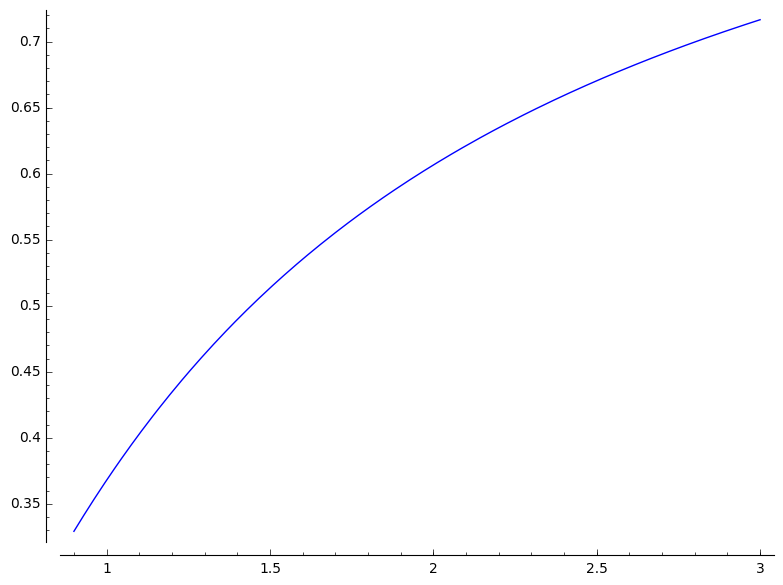
which we can solve for . Thus, the optimal number of initial rejections is approximately for sufficiently large. A plot is shown in Figure 4.
 |
5.2. Optimal probability of success
Reviewing the previous section, we find that we can solve explicitly. Each polynomial is just a constant in (that depends on and ) times the polynomial .
Theorem 5.1.
For all and , we have
When , we have .
Proof.
This is straightforward to prove by induction from Theorem 4.3. ∎
Since the optimal value of satisfies we can cancel it and the optimal probability simplifies to
When is an integer, this is just a ratio of binomial coefficients, but for arbitrary positive real we use gamma functions (see e.g. [OLBC10]). By iterating the recurrence we obtain . Hence,
Using , we get
Remarkably, this probability of success is independent of .
6. Results for Mallows distribution
We now turn to the Mallows distribution defined by inversions in . We begin by working out the standard “-analogue” for this statistic.
Definition 6.1.
Let be the polynomial in defined by . Let be the polynomial in defined by
Lemma 6.2.
We have
Proof.
This is straightforward to prove using induction since we may extend each permutation of by placing one of the values in the last position and arranging the complementary values according to . This creates new inversions, so contributes to . ∎
Let us redefine
for the Mallows distribution. Our next result provides a recursive description for these polynomials.
Theorem 6.3.
We have
with initial conditions and .
Proof.
We have two cases for the -winnable permutations .
-
•
If the last position contains one of the values , then it contributes to the inversion count and we may view the complementary values as some -winnable . Hence, these contribute to .
-
•
If the last position contains then the value must lie in one of the first positions in order for to be -winnable. These choices for the position of value contribute . For each of these, we choose a permutation of size to fill in the remaining positions, keeping track of the inversions with .
The initial conditions are immediate. ∎
We can solve this recurrence.
Corollary 6.4.
We have
for and .
Proof.
This is straightforward to prove by induction on from Theorem 6.3. ∎
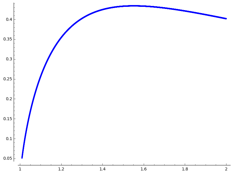
For this distribution, the precise transition probabilities for each seem to be inaccessible, being roots of polynomials (with complex solutions) that use many repeated root extractions as opposed to the rational numbers we obtained in the Ewens case. However, we obtain some interesting asymptotic results. Figure 5 shows a plot of the optimal success probability for various values of based on the following theorem.
 |
Theorem 6.5.
If then the optimal strategy as becomes large is to reject the first candidates where , and select the next left-to-right maximum thereafter. This strategy succeeds with probability . If , this probability of success simplifies to .
Proof.
For fixed , as becomes large, the fraction tends to and the terms in the series become close to so the probability reduces to . This sequence converges to a positive value if and only if the sequence converges to a finite value.
So we let obtaining . Differentiating with respect to and setting equal to zero, we solve to obtain the optimal . For , we have but we cannot reject more than candidates so max appears in the expression. ∎
The case where is less interesting from our intrinsic learning perspective but we sketch the behavior of these models for mathematical completeness. Taken together, the results also prove that the asymptotically optimal strategy does not vary continuously with the parameter .
|
Corollary 6.6.
Fix and an integer . Then,
In particular, we approach a single asymptotic distribution as so the optimal strategy will be to reject some number of initial candidates (not depending on ) and select the next left-to-right maximum thereafter.
Proof.
Once again, consider
For fixed , as becomes large, the fraction tends to and the series converges (e.g. by the integral test).
Thus, every -positional strategy has some nonzero probability in the limit as . As becomes large, the series tends to zero, being approximately . Therefore, the optimal asymptotic probability will occur for some fixed (depending on ). ∎
Figure 6 shows some plots (obtained numerically) of the optimal success probabilities for various values of and . For any particular value of , one can explicitly compute the probabilities in Corollary 6.6 and find the optimal strategy . For example, it appears that is optimal for all (approximately). Although the series always converges, finding a closed form for its limiting value involves the “-digamma function” which prevents us from obtaining a simple description of the optimal strategy in general. It also appears that the maximal probability of success for these models occurs when (for which is the optimal strategy). It would be interesting to determine this maximum more precisely.
Acknowledgements
We thank Laura Taalman, John Webb, and Becky Wild for helpful discussions related to this work.
References
- [ABNP16] Nicolas Auger, Mathilde Bouvel, Cyril Nicaud, and Carine Pivoteau, Analysis of algorithms for permutations biased by their number of records, Proceedings of the 27th International Conference on Probabilistic, Combinatorial and Asymptotic Methods for the Analysis of Algorithms—AofA’16, Jagiellonian Univ., Dep. Theor. Comput. Sci., Kraków, 2016, p. 12. MR 3817514
- [ABT03] Richard Arratia, A. D. Barbour, and Simon Tavaré, Logarithmic combinatorial structures: a probabilistic approach, EMS Monographs in Mathematics, European Mathematical Society (EMS), Zürich, 2003. MR 2032426
- [BIKR08] M. Babaioff, N. Immorlica, D. Kempe, and Kleinberg R., Online auctions and generalized secretary problems, SIGecom Exchange 7 (2008), 1–11.
- [CDE18] Harry Crane, Stephen DeSalvo, and Sergi Elizalde, The probability of avoiding consecutive patterns in the Mallows distribution, Random Structures Algorithms 53 (2018), no. 3, 417–447. MR 3854041
- [Fer89] Thomas S. Ferguson, Who solved the secretary problem?, Statist. Sci. 4 (1989), no. 3, 282–296, With comments and a rejoinder by the author. MR 1015277
- [FJ19] Aaron Fowlkes and Brant Jones, Positional strategies in games of best choice, Involve 12 (2019), no. 4, 647–658. MR 3941603
- [Fre83] P. R. Freeman, The secretary problem and its extensions: a review, Internat. Statist. Rev. 51 (1983), no. 2, 189–206.
- [Gar95] Martin Gardner, New mathematical diversions, revised ed., MAA Spectrum, Mathematical Association of America, Washington, DC, 1995. MR 1335231
- [GM66] John P. Gilbert and Frederick Mosteller, Recognizing the maximum of a sequence, J. Amer. Statist. Assoc. 61 (1966), 35–73. MR 0198637
- [Jon19] Brant Jones, Avoiding patterns and making the best choice, Discrete Math. 342 (2019), no. 6, 1529–1545. MR 3922151
- [Kad94] Richard V. Kadison, Strategies in the secretary problem, Exposition. Math. 12 (1994), no. 2, 125–144. MR 1274782
- [OLBC10] Frank W. J. Olver, Daniel W. Lozier, Ronald F. Boisvert, and Charles W. Clark (eds.), NIST handbook of mathematical functions, U.S. Department of Commerce, National Institute of Standards and Technology, Washington, DC; Cambridge University Press, Cambridge, 2010, With 1 CD-ROM (Windows, Macintosh and UNIX). MR 2723248
- [Pal58] R. Palermo, Addendum to a letter by Merrill R. Flood, Martin Gardner papers at Stanford University Archives (1958), series 1, box 5, folder 19.
- [Pfe89] Dietmar Pfeifer, Extremal processes, secretary problems and the law, J. Appl. Probab. 26 (1989), no. 4, 722–733. MR 1025389
- [RF88] J. H. Reeves and V. F. Flack, A generalization of the classical secretary problem: dependent arrival sequences, J. Appl. Probab. 25 (1988), no. 1, 97–105. MR 929508
- [SV99] Dimitris A. Sardelis and Theodoros M. Valahas, Decision making: a golden rule, Amer. Math. Monthly 106 (1999), no. 3, 215–226. MR 1682342