Variational neural network ansatz for steady states in open quantum systems

Abstract

We present a general variational approach to determine the steady state of open quantum lattice systems via a neural network approach. The steady-state density matrix of the lattice system is constructed via a purified neural network ansatz in an extended Hilbert space with ancillary degrees of freedom. The variational minimization of cost functions associated to the master equation can be performed using a Markov chain Monte Carlo sampling. As a first application and proof-of-principle, we apply the method to the dissipative quantum transverse Ising model.

In spite of the tremendous experimental progress in the isolation of quantum systems, a finite coupling to the environment Breuer and Petruccione (2007) is unavoidable and certainly plays a crucial role in the practical implementation of quantum information and quantum simulation protocols Devoret and Schoelkopf (2013). Moreover, through an active control of the environment via the so-called reservoir engineering, an open quantum manybody system can be prepared in non-trivial phases Carusotto and Ciuti (2013); Noh and Angelakis (2016); Hartmann (2016) with also possible quantum applications Verstraete et al. (2009); Barreiro et al. (2011). The theoretical description of open quantum manybody systems is in general out-of-the equilibrium and much less developed than for equilibrium systems. A mixed state with a finite entropy can be described by a density matrix, whose evolution is described by a master equation. Recently, a few theoretical methods have been developed to solve the master equation of open quantum manybody systems, including analytical approaches based on the Keldysh formalism Sieberer et al. (2016); Maghrebi and Gorshkov (2016), numerical algorithms based on matrix product operator and tensor-network techniques Mascarenhas et al. (2015); Cui et al. (2015); Jaschke et al. (2019); Werner et al. (2016); Kshetrimayum et al. (2017), cluster mean-field methods Biella et al. (2018); Jin et al. (2016), corner-space renormalization Finazzi et al. (2015); Rota et al. (2017, 2018), Gutzwiller mean-field Casteels et al. (2018), full configuration-interaction Monte Carlo Nagy and Savona (2018), permutation-invariant solvers Shammah et al. (2018) or efficient stochastic unravelings for disordered systems Vicentini et al. (2018). The research in the field is very active, since the different methods are optimal for different specific regimes. For example, the corner-space renormalization method is best suited for systems with moderate entropy, while matrix product operator techniques to systems with short-range quantum correlations.

In the last decade, the field of artificial neural networks has enjoyed a dramatic expansion and success thanks to remarkable applications in the recognition of complex patterns such as visual images or human speech (for a recent review see, e.g., LeCun et al. (2015)). The optimization (supervised learning) of the network is obtained by tuning the weights quantifying the connections between neural units via a variational minimization of a properly defined cost function. The wavefunction of a manybody system is in general a complex quantity, which is hard to be recognized. Recent works have proposed to exploit artificial neural networks to construct trial wavefunctions, where the connection weights in the network play the role of variational parameters Carleo and Troyer (2017); Glasser et al. (2018). Neural network approaches have already been succesffuly applied to a wide number (see e.g. van Nieuwenburg et al. (2017); Schindler et al. (2017); Choo et al. (2018); Czischek et al. (2018); Sharir et al. (2019)) of close Hamiltonian systems. However, they have not yet been generalized to the important quantum manybody problem of open systems.

In this Letter, we present a theoretical approach based on a variational neural network ansatz in order to determine the steady state of the master equation of open quantum lattice systems. We construct the ansatz for the mixed density matrix starting from a Restricted Boltzman Machine ansatz for a pure many-body wavefunction in an extended Hilbert space. We determine the optimal variational parameters by minimizing a cost function which involves the Liouvillian superoperator associated to the master equation for the density matrix. As a first application, we have considered the dissipative tranverse field quantum Ising model. We present a proof-of-principle demonstration by benchmarking the neural network calculations of the steady state against numerically exact simulations performed by quantum trajectories in the full Hilbert space Daley (2014). Our minimization of the cost function is performed by Markov chain Monte Carlo sampling of the gradient and is thus scalable to a large number of lattice sites. Perspectives of the present approach are discussed in the conclusions.

The general task that we wish to solve is the determination of the steady state of an open quantum system described by the Lindblad master equation Breuer and Petruccione (2007) for the system reduced density matrix $\hat{\rho}$, which reads (setting $\hbar=1$):

$$\dot{\hat{\rho}}=\mathcal{L}\hat{\rho}=-i\commutator{\hat{H}}{\hat{\rho}}+\sum_{j}\frac{\gamma_{j}}{2}\left[2\hat{L}_{j}\hat{\rho}\hat{L}^{\dagger}_{j}-\{\hat{L}_{j}^{\dagger}\hat{L}_{j},\hat{\rho}\}\right],$$ (1)

where $\mathcal{L}$ is the so-called Liouvillian superoperator depending on the system Hamiltonian operator $\hat{H}$. The coupling to the environment is represented by interaction channels with the reservoir characterized by dissipation rates $\gamma_{j}$ and jump operators $\hat{L}_{j}$ acting on the system. Here we will focus on situations where the steady state ($\partial_{t}\hat{\rho}_{ss}=0$) is unique. In this case, the steady-state density matrix can be obtained as $\hat{\rho}_{ss}=\lim_{t\rightarrow\infty}\hat{\rho}(t)$ regardless of the initial condition. Although it is possible to engineer peculiar Liouvillians with more than one steady state Albert and Jiang (2014), typical physical systems with a finite Hilbert space dimension have a unique steady-state Spohn (1977); Minganti et al. (2018); Nigro_2019Nigro_2019.

For the many-body problem an analytical expression for $\hat{\rho}_{ss}$ can be found in very few cases Prosen (2014, 2011). In general, because of the exponential growth of the Hilbert space with the number of lattice sites, describing the full density matrix requires exponentially many complex numbers, which in practice can be done exactly only for a small number of sites. If one wants to attack the problem within a variational framework, the density matrix can be represented by an ansatz $\hat{\rho}_{\bm{v}}$ depending on a set of variational parameters ${\bm{v}}$. If $\{\ket{{\bm{\sigma}}}=\ket{\sigma_{1},\sigma_{2},...,\sigma_{N}}\}$ denotes a basis of states for the system Hilbert space, the density matrix can be expressed in the form

$$\hat{\rho}({\bm{v}})=\sum_{\bm{\sigma},\bm{\sigma^{\prime}}}\rho_{\bm{v}}({\bm{\sigma}},\bm{\sigma^{\prime}})\ket{\bm{\sigma}}\bra{\bm{\sigma}^{\prime}}.$$ (2)

In order to construct our neural network ansatz for the density matrix, we consider an extended Hilbert space $\mathcal{H}=\mathcal{H}_{S}\otimes\mathcal{H}_{A}$ where $\mathcal{H}_{S,A}$ represents respectively the system and ancillary Hilbert spaces. Such extended space is spanned by the basis set $\{\ket{{\bm{\sigma}},{\bm{a}}}\}$ where ${\bm{a}}=({a_{1},a_{2},...,a_{N_{a}}})$ labels the ancillary degrees of freedom. We start by considering a pure state in the extended Hilbert space, represented by the wavefunction $\psi_{\bm{v}}({\bm{\sigma}},{\bm{a}})$. In this framework the reduced density matrix of the system $S$ is obtained by tracing out the ancillary degrees freedom Torlai and Melko (2018), namely

$$\rho_{\bm{v}}(\bm{\sigma},{\bm{\sigma}^{\prime}})=\sum_{\bm{a}}\psi_{\bm{v}}({\bm{\sigma}},{\bm{a}})\psi_{\bm{v}}^{\star}({\bm{\sigma}^{\prime}},{\bm{a}}).$$ (3)

The next step is to represent $\psi_{\bm{v}}({\bm{\sigma}},{\bm{a}})$ via a neural network ansatz. This purified procedure automatically ensures that $\hat{\rho}_{\bm{v}}$ is Hermitian and positive semi-definite, as required for a density matrix. In a recent paper, Torlai and Melko Torlai and Melko (2018) proposed to describe purified wavefunctions as

$$\psi_{\bm{v}}({\bm{\sigma}},{\bm{a}})=\sqrt{{\mathcal{P}}_{{\bm{v}}_{A}}({\bm{\sigma}},{\bm{a}})}\exp[-1/2\log({\mathcal{P}}_{{\bm{v}}_{\theta}}({\bm{\sigma}},{\bm{a}}))].$$ (4)

Both the amplitude ${\mathcal{P}}_{{\bm{v}}_{A}}({\bm{\sigma}},{\bm{a}})$ and phase-related function ${\mathcal{P}}_{{\bm{v}}_{\theta}}({\bm{\sigma}},{\bm{a}})$ of the purified wavefunction are given by the Boltzmann-like expression ${\mathcal{P}}_{\nu}({\bm{\sigma}},{\bm{a}})=\sum_{\bm{h}}\exp[-E_{\nu}({\bm{\sigma}},{\bm{a}},{\bm{h}})]$ (with $\nu\in\{\bm{v}_{A},\bm{v}_{\theta}\}$), where the associated dimensionless energy reads

$$E_{\nu}({\bm{\sigma}},{\bm{a}},{\bm{h}})={\bm{\sigma}}\cdot{\bf{b}}^{(\sigma)}_{\nu}+{\bm{a}}\cdot{\bm{b}}^{(a)}_{\nu}+{\bm{h}}\cdot{{\bm{b}}}^{(h)}_{\nu}+{\bm{\sigma}}^{T}{{\bm{W}}}_{\nu}{\bm{h}}+{\bm{\sigma}}^{T}{{\bm{U}}}_{\nu}{\bm{a}}.$$ (5)

Note that the ansatz parameters are ${\bm{v}}=({\bm{v}}_{A},{\bm{v}}_{\theta})$ where ${\bm{v}}_{\nu}=({\bf{b}}^{(\sigma)}_{\nu},{\bm{b}}^{(a)}_{\nu},{{\bm{b}}}^{(h)}_{\nu},{{\bm{W}}}_{\nu},{{\bm{U}}}_{\nu})$. The rectangular matrix ${{\bm{W}}}_{\nu}$ weighs the connections between the system variables (visible layer) to the auxiliary variables (hidden layer), while the weight matrix ${{\bm{U}}}_{\nu}$ quantifies the connection between the system variables and the ancillary ones (ancillary layer). Such neural network ansatz is represented by a tri-partite Restricted Boltzmann Machine depicted in fig. 1. In other words, there are two independent artificial neural networks, one for the amplitude ($\nu=A$) and one for the phase ($\nu=\theta$). By substituting those formulas into Eq. 3 and carrying out the sum over the ancillary degrees of freedom one obtains a closed formula for the entries of the density matrix:

$$\rho_{{\bm{v}}}({{\bm{\sigma}},{\bm{\sigma}^{\prime}}})=\exp[\Gamma^{-}_{\bm{v}}(\bm{\sigma},\bm{\sigma^{\prime}})+\Gamma^{+}_{\bm{v}}({{\bm{\sigma}},{\bm{\sigma}^{\prime}}})+\Pi_{\bm{v}}({{\bm{\sigma}},{\bm{\sigma}^{\prime}}})]$$ (6)

where the expression of $\Gamma^{+/-}$ and $\Pi$ can be found in the Supplemental Material . The representation power Roux and Bengio (2008); Younes (1996); Montufar and Ay (2011) of this ansatz can be systematically improved by increasing the density of the hidden ($\alpha=N_{h}/N$) and ancillary layer ($\beta=N_{a}/N$). It is worth pointing out that this scheme is not specific to this network topology, but relies only on the general fact that if two visible layers are connected by a shallow ancillary layer, the ancilla can be traced out analitically and an efficient neural-network description of the density matrix can be obtained.

[width=]NDM

Figure 1: Graph representation of the artificial neural network used for the density matrix ansatz. The vector ${\bm{\sigma}}=(\sigma_{1},\sigma_{2},...,\sigma_{N})$ contains the variables of the physical system (visible layer). The vector ${\bm{a}}=(a_{1},a_{2},...,\sigma_{N_{a}})$ describes the ancillary degrees of freedom of the extended Hilbert space (ancilla layer), where a purified density matrix is considered (see Eq. (3)). The vector ${\bm{h}}=(h_{1},h_{2},...,h_{N_{h}})$ contains variables of auxiliary nodes (hidden layer). The network parameters are ${\bm{v}}_{\nu}=({\bf{b}}^{(\sigma)}_{\nu},{\bm{b}}^{(a)}_{\nu},{{\bm{b}}}^{(h)}_{\nu},{{\bm{W}}}_{\nu},{{\bm{U}}}_{\nu})$. One network is used for the representation of the amplitude ($\nu=\bm{v}_{A}$) of the purified wavefunction in Eq. (3), while another independent network with the same topology is used to represent the phase ($\nu=\bm{v}_{\theta}$).

Having defined a variational ansatz $\hat{\rho}(\bm{v})$, we now wish to define a variational principle to determine the optimal parameters. In particular, we have to recast the search for the steady state into a minimization problem for a real, positive cost function $\mathcal{C}({\bm{v}})$ which has a global minimum when the master equation ${\mathcal{L}}\hat{\rho}_{{\bm{v}}}=0$ is satisfied Weimer (2015). Moreover, in order to be able to deal with large Hilbert spaces, we need a quantity which can be sampled and computed efficiently. These requirements are met by the following cost function expressed in terms of the 2-norm of the time derivative of the density-matrix:

$$\mathcal{C}({\bm{v}})=\frac{\norm{d\hat{\rho}_{\bm{v}}/dt}^{2}_{2}}{\norm{\hat{\rho}_{\bm{v}}}^{2}_{2}}=\frac{\Tr[\hat{\rho}^{\dagger}_{\bm{v}}\mathcal{L^{\dagger}}\mathcal{L}\hat{\rho}_{\bm{v}}]}{\Tr[\hat{\rho}^{\dagger}_{\bm{v}}\hat{\rho}_{\bm{v}}]},$$ (7)

as (i) $\mathcal{C}({\bm{v}}_{ss})=0\iff\hat{\rho}({\bm{v}}_{ss})=\hat{\rho}_{ss}$ and (ii) $\mathcal{C}({\bm{v}})\geq 0$.

It is useful to rewrite Eq. 7 as a sum over the whole space of bounded operators on the Hilbert space:

$$\mathcal{C}({\bm{v}})=\sum_{\bm{\sigma},\bm{\tilde{\sigma}}}p_{\bm{v}}(\bm{\sigma},\bm{\tilde{\sigma}})|\mathcal{C}^{\text{Loc}}(\bm{v},\bm{\sigma},\bm{\tilde{\sigma}})|^{2},$$ (8)

where $p_{\bm{v}}(\bm{\sigma},\bm{\tilde{\sigma}})=\absolutevalue{\rho_{\bm{v}}(\bm{\sigma},\bm{\tilde{\sigma}})}^{2}/Z$ corresponds to a probability distribution as $Z=\sum_{\bm{\sigma},\bm{\tilde{\sigma}}}\absolutevalue{\rho_{\bm{v}}(\bm{\sigma},\bm{\tilde{\sigma}})}^{2}$ . The local contribution reads :

$$\mathcal{C}^{\text{Loc}}(\bm{v},\bm{\sigma},\bm{\tilde{\sigma}})=\sum_{\bm{\sigma}^{\prime},\bm{\tilde{\sigma}}^{\prime}}\mathcal{L}(\bm{\sigma},\bm{\tilde{\sigma}};\bm{\sigma}^{\prime},\bm{\tilde{\sigma}}^{\prime})\frac{\rho_{\bm{v}}(\bm{\sigma}^{\prime},\bm{\tilde{\sigma}}^{\prime})}{\rho_{\bm{v}}(\bm{\sigma},\bm{\tilde{\sigma}})}.$$ (9)

In order to find the global minimum of the cost function (7) by means of gradient-based iterative schemes we need to compute its gradient

$$\nabla_{\bm{v}}\ \mathcal{C}({\bm{v}})=\sum_{\bm{\sigma},\bm{\tilde{\sigma}}}p_{\bm{v}}(\bm{\sigma},\bm{\tilde{\sigma}})\mathcal{C}^{\text{Loc}}(\bm{v},\bm{\sigma},\bm{\tilde{\sigma}})^{\star}\Big{[}\sum_{\sigma^{\prime},\tilde{\sigma}^{\prime}}\mathcal{L}(\bm{\sigma},\bm{\tilde{\sigma}};\bm{\sigma}^{\prime},\bm{\tilde{\sigma}}^{\prime})\cr\frac{\rho_{\bm{v}}(\bm{\sigma}^{\prime},\bm{\tilde{\sigma}}^{\prime})}{\rho_{\bm{v}}(\bm{\sigma},\bm{\tilde{\sigma}})}\mathcal{O}_{\bm{v}}(\bm{\sigma}^{\prime},\bm{\tilde{\sigma}}^{\prime})\Big{]}-\mathcal{C}(\bm{v})\mathcal{O}_{\bm{v}},$$ (10)

where we have defined the log-derivatives of the density matrix $\mathcal{O}_{\bm{v}}=\sum_{\bm{\sigma},\bm{\tilde{\sigma}}}\mathcal{O}_{\bm{v}}(\bm{\sigma},\bm{\tilde{\sigma}})$ and $\mathcal{O}_{\bm{v}}(\bm{\sigma},\bm{\tilde{\sigma}})=\nabla_{\bm{v}}\log{\rho_{\bm{v}}(\bm{\sigma},\bm{\tilde{\sigma}})}$, which can be efficiently computed for the considered neural network.

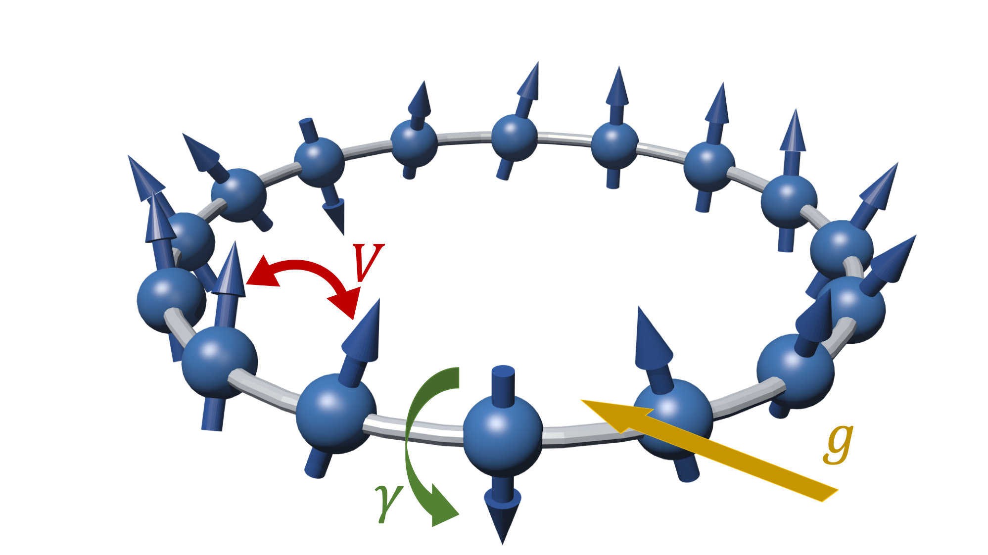
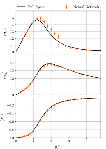
Figure 2: Top panel: sketch of the considered physical system described by the dissipative quantum transverse Ising 1D model with periodic boundary conditions. The quantity $g$ denotes an applied magnetic field, $V$ the spin-spin coupling and $\gamma$ the spin flip rate. Bottom panel: the prediction of the neural-network variational calculations (circles) are compared to the results obtained by quantum trajectory simulations of the master equation by considering the whole Hilbert space (solid lines). The top, middle and bottom panels depict the expectation values of the three components of the averaged magnetization as a function of the applied magnetic field $g$ (in units of $\gamma$). Model parameters: $V/\gamma=2$ (spin-spin coupling), $N=16$ (number of lattice sites). Neural-network parameters: $\alpha=\beta=1$ for $g\leq\gamma$ and $g\geq 2.5\gamma$ while $\alpha=1$ and $\beta=4$ for the remaining points. The parameters required for the convergence of the Monte Carlo calculations depend on the value of $g/\gamma$, with the intermediate region being the most demanding. The maximum number of accepted Monte Carlo samples is $8640$ and the maximum number of steps for the stochastic gradient descent is $10^{4}$. For points outside the intermediate region $3000$ accepted Monte Carlo samples and $10^{3}$ iteration steps have been performed.

The computational complexity of evaluating $\nabla\mathcal{C}({\bm{v}})$ exactly grows exponentially with the size of the system. This cost can be considerably reduced if one only uses an estimate of $\nabla\mathcal{C}({\bm{v}})$ obtained by sampling the values $(\bm{\sigma},\bm{\tilde{\sigma}})$ according to the probability $p_{\bm{v}}(\bm{\sigma},\bm{\tilde{\sigma}})$. Because the normalisation factor $Z$ is not fixed, we cannot sample the distribution directly and have to resort to a Markov Chain Monte Carlo Becca and Sorella (2017a) with Metropolis update rules . At every sampling step, we propose to update the configuration $(\bm{\sigma},\bm{\tilde{\sigma}})\rightarrow(\bm{\sigma}^{\prime},\bm{\tilde{\sigma}}^{\prime})$ by switching a random number of spins and accept the new configuration with probability $\min(\exp[p_{\bm{v}}(\bm{\sigma},\bm{\tilde{\sigma}})/p_{\bm{v}}(\bm{\sigma}^{\prime},\bm{\tilde{\sigma}}^{\prime})],1)$.

Finally, in order to find the global minimum of the cost function we employ a standard Stochastic Gradient Descent algorithm Bottou (2010). In order to improve the performance of the Stochastic Gradient Descent (i.e. to reduce the number of iterations needed to converge to the global minima of the cost function) we update the variational parameters according to to the metric of the space of density matrices exploiting the Stochastic Reconfiguration Approach Becca and Sorella (2017b). During the optimization procedure we sample the physical observables of interest through another Markov chain as

$$\expectationvalue*{\hat{\Theta}}=\frac{\Tr[\hat{\rho}\ \hat{\Theta}]}{\Tr[\hat{\rho}]}=\sum_{\bm{\sigma}}p^{\rm obs}_{\bm{v}}(\bm{\sigma})\sum_{\bm{\tilde{\sigma}}}\frac{\rho_{\bm{v}}(\bm{\sigma},\bm{\tilde{\sigma}})\Theta(\bm{\tilde{\sigma}},\bm{\sigma})}{\rho_{\bm{v}}(\bm{\sigma},\bm{\sigma})},$$ (11)

where $p^{\rm obs}_{\bm{v}}(\bm{\sigma})=\rho_{\bm{v}}(\bm{\sigma},\bm{\sigma})/\Tr[\hat{\rho}]$.

In order to benchmark our neural-network approach for open quantum systems, we consider here the dissipative quantum transverse Ising model, whose Hamiltonian is

$$H=\frac{V}{4}\sum_{\langle j,l\rangle}\hat{\sigma}^{z}_{j}\hat{\sigma}_{l}^{z}+\frac{g}{2}\sum_{j}\hat{\sigma}_{j}^{x},$$ (12)

being $\hat{\sigma}_{j}^{\alpha}$ the Pauli matrices ($\alpha\in\{x,y,z\}$) acting on the $j$-th site. The first term represents the nearest-neighbor spin-spin interaction depending only on the $z$-components, being $V$ the coupling strength. The second term accounts for a local and uniform magnetic field along the transverse direction $x$. We consider local dissipative spin-flip processes described by the site-dependent jump operator $\hat{L}_{j}^{(z)}=\hat{\sigma}_{j}^{-}=\frac{1}{2}(\hat{\sigma}^{x}_{j}-i\hat{\sigma}^{y}_{j})$, which fully determine the master equation in Eq. (1).

Numerical results for steady-state observables of the dissipative quantum transverse Ising model on a 1D periodic chain are reported in Fig. 2. In particular, we report the spatial components of the averaged magnetization as a function of the magnetic field $g$ (in units of the dissipation rate $\gamma$) for $V/\gamma=2$. For $N=16$ lattice sites the predictions of the neural-network variational method (circles) are compared to the results obtained with a brute-force exact integration of the master equation in the whole Hilbert space, showing a good agreement over all the parameter range. For $g\lesssim\gamma$ and $g\gtrsim 2.5\gamma$ a remarkable precision is reached for all the local observables with a low density of the hidden and ancillary layer $\alpha=\beta=1$ and $\mathcal{O}(10^{2})$ minimization steps. For $1\lesssim g/\gamma\lesssim 2.5$ an higher number of variational parameters is required. In particular, as shown in Fig. 3, a systematic improvement of the relative error $\epsilon_{\rm rel}\big{[}\expectationvalue{\sigma_{x}}\big{]}$ with respect to the exact solution can be obtained by increasing $\beta$. Interestingly, for $1\lesssim g/\gamma\lesssim 2.5$, we note that the gradient-descent procedure requires more iterations. This region corresponds to the range of $g/\gamma$ where the smallest nonzero eigenvalue of $\mathcal{L^{\dagger}}\mathcal{L}$ decreases significantly Jin et al. (2018). In this range the steady-state density matrix also displays nontrivial correlations and non-thermal mixness properties Jin et al. (2018). Remarkably, the fidelity of the reconstructed local density matrix with respect to the exact one is alway larger then $0.998$ for all the values of $g/\gamma$ considered.

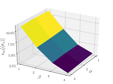
Figure 3: Relative error with respect to the exact result for the observable $\expectationvalue{\sigma_{x}}$ as a function of $\alpha$ and $\beta$. Parameters are set as in Fig.2 but for a fixed value $g/\gamma=1.2$.

Finally, as an example of convergence, the top panel of Fig. 4 depicts a typical evolution of the cost function in the iterative minimization procedure for a fixed set of parameters ($g/\gamma=1$), showing a good convergence towards the global minimum. In the bottom panel of Fig. 4, the convergence of the $x$-component of the averaged magnetization is also reported.

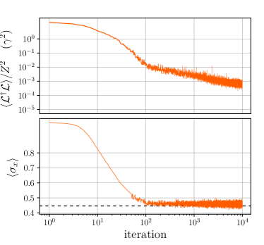
Figure 4: Same parameters as in Fig. 2 but for a fixed value $g/\gamma=1$. Top panel: the cost function is shown as a function of the iteration steps. Bottom panel: the corresponding evolution of the $x$-component of the average magnetization during the stochastic minimization is shown.

In conclusion, we have presented a general variational approach for the steady-state density matrix of open quantum manybody systems based on an artificial neural network scheme. Our method is scalable since the cost function associated to the Liouvillian of the master equation can be calculated via Monte Carlo sampling. We have demonstrated a proof-of-principle of the theoretical scheme by a successful benchmarking to brute-force finite-size simulations in the full Hilbert space for arrays of spins described by the dissipative quantum transverse Ising model. We would like to point out that the present approach does not depend on the specific network topology. Indeed, the variational procedure presented in this Letter is general and can be applied to many other neural-networks or physically-inspired variational ansätze. There are many future developments at the horizon, including the study of dynamical properties, the use of deep neural networks and/or alternative cost functions, comparison with other existing techniques as well as the study of disordered systems without translational invariance. The neural network approach has the potential to pave the way to the theoretical study of a wide spectrum of open quantum manybody systems.

See pages 1 of SupMat.pdf See pages 2 of SupMat.pdf See pages 3 of SupMat.pdf See pages 4 of SupMat.pdf See pages 5 of SupMat.pdf