Perturbed-History Exploration in Stochastic Multi-Armed Bandits

Abstract

We propose an online algorithm for cumulative regret minimization in a stochastic multi-armed bandit. The algorithm adds $O(t)$ i.i.d. pseudo-rewards to its history in round $t$ and then pulls the arm with the highest average reward in its perturbed history. Therefore, we call it perturbed-history exploration (${\tt PHE}$). The pseudo-rewards are carefully designed to offset potentially underestimated mean rewards of arms with a high probability. We derive near-optimal gap-dependent and gap-free bounds on the $n$-round regret of ${\tt PHE}$. The key step in our analysis is a novel argument that shows that randomized Bernoulli rewards lead to optimism. Finally, we empirically evaluate ${\tt PHE}$ and show that it is competitive with state-of-the-art baselines.

1 Introduction

A multi-armed bandit Lai and Robbins (1985); Auer et al. (2002); Lattimore and Szepesvari (2019) is an online learning problem where actions of the learning agent are represented by arms. After the arm is pulled, the agent receives its stochastic reward. The objective of the agent is to maximize its expected cumulative reward. The agent does not know the mean rewards of the arms in advance and faces the so-called exploration-exploitation dilemma: explore, and learn more about the arm; or exploit, and pull the arm with the highest average reward thus far. The arm may be a treatment in a clinical trial and its reward is the outcome of that treatment on some patient population.

Thompson sampling (TS) Thompson (1933); Russo et al. (2018) and optimism in the face of uncertainty (OFU) Auer et al. (2002); Dani et al. (2008); Abbasi-Yadkori et al. (2011) are the most celebrated and studied exploration strategies in stochastic multi-armed bandits. These strategies are near optimal in multi-armed Garivier and Cappe (2011); Agrawal and Goyal (2013a) and linear Abbasi-Yadkori et al. (2011); Agrawal and Goyal (2013b) bandits. However, they typically do not generalize easily to complex problems. For instance, in generalized linear bandits Filippi et al. (2010), we only know how to construct approximate high-probability confidence sets and posterior distributions. These approximations affect the statistical efficiency of bandit algorithms Filippi et al. (2010); Zhang et al. (2016); Abeille and Lazaric (2017); Jun et al. (2017); Li et al. (2017). In online learning to rank Radlinski et al. (2008), we only have statistically efficient algorithms for simple user interaction models, such as the cascade model Kveton et al. (2015); Katariya et al. (2016). If the model was a general graphical model with latent variables Chapelle and Zhang (2009), we would not know how to design a bandit algorithm with regret guarantees. In general, efficient approximations to high-probability confidence sets and posterior distributions are hard to design Gopalan et al. (2014); Kawale et al. (2015); Lu and Van Roy (2017); Riquelme et al. (2018); Lipton et al. (2018); Liu et al. (2018).

In this work, we propose a novel exploration strategy that is conceptually straightforward and has the potential to easily generalize to complex problems. In round $t$, the learning agent adds $O(t)$ i.i.d. pseudo-rewards to its history and treats them as if they were generated by actual arm pulls. Then the agent pulls the arm with the highest average reward in this perturbed history and observes the reward of the pulled arm. The pseudo-rewards are drawn from the same family of distributions as actual rewards, but generate maximum variance randomized data.

Our algorithm, perturbed-history exploration (${\tt PHE}$), is inherently optimistic. To see this, note that the lack of optimism regarding arm $i$ in round $t$, that its estimated mean reward is below the actual mean, is due to a specific history of past $O(t)$ rewards. These rewards are independent noisy realizations of the mean reward of arm $i$. Therefore, the lack of optimism can be offset by adding $O(t)$ i.i.d. pseudo-rewards to the history of arm $i$, so that the estimated mean reward of arm $i$ in its perturbed history is above the mean with a high probability. This design is conceptually simple and appealing, because maximum variance rewards can be easily generated for any reward generalization model.

We make the following contributions in this paper. First, we propose ${\tt PHE}$, a multi-armed bandit algorithm where the mean rewards of arms are estimated using a mixture of actual rewards and i.i.d. pseudo-rewards. Second, we analyze ${\tt PHE}$ in a $K$-armed bandit with $[0,1]$ rewards, and prove both $O(K\Delta^{-1}\log n)$ and $O(\sqrt{Kn\log n})$ bounds on its $n$-round regret, where $\Delta$ is the minimum gap between the mean rewards of the optimal and suboptimal arms. The key to our analysis is a novel argument that shows that randomized Bernoulli rewards lead to optimism. Finally, we empirically compare ${\tt PHE}$ to several baselines and show that it is competitive with the best of them.

2 Setting

We use the following notation. The set $\left\{1,\dots,n\right\}$ is denoted by $[n]$. We define $\mathrm{Ber}(x;p)=p^{x}(1-p)^{1-x}$ and let $\mathrm{Ber}(p)$ be the corresponding Bernoulli distribution. We also define $B(x;n,p)=\binom{n}{x}p^{x}(1-p)^{n-x}$ and let $B(n,p)$ be the corresponding binomial distribution. For any event $E$, $\mathds{1}\!\left\{E\right\}=1$ if and only if event $E$ occurs, and is zero otherwise.

We study the problem of cumulative regret minimization in a stochastic multi-armed bandit. Formally, a stochastic multi-armed bandit Lai and Robbins (1985); Auer et al. (2002); Lattimore and Szepesvari (2019) is an online learning problem where the learning agent sequentially pulls $K$ arms in $n$ rounds. In round $t\in[n]$, the agent pulls arm $I_{t}\in[K]$ and receives its reward. The reward of arm $i\in[K]$ in round $t$, $Y_{i,t}$, is drawn i.i.d. from a distribution of arm $i$, $P_{i}$, with mean $\mu_{i}$ and support $[0,1]$. The goal of the agent is to maximize its expected cumulative reward in $n$ rounds. The agent does not know the mean rewards of the arms in advance and learns them by pulling the arms.

Without loss of generality, we assume that the first arm is optimal, that is $\mu_{1}>\max_{i>1}\mu_{i}$. Let $\Delta_{i}=\mu_{1}-\mu_{i}$ denote the gap of arm $i$. Maximization of the expected cumulative reward in $n$ rounds is equivalent to minimizing the expected $n$-round regret, which we define as

$$R(n)=\sum_{i=2}^{K}\Delta_{i}\mathbb{E}\left[\sum_{t=1}^{n}\mathds{1}\!\left\{I_{t}=i\right\}\right]\,.$$

3 Perturbed-History Exploration

Our new algorithm, perturbed-history exploration (${\tt PHE}$), is presented in Algorithm 1. ${\tt PHE}$ pulls the arm with the highest average reward in its perturbed history, which is estimated as follows. Let $T_{i,t}=\sum_{\ell=1}^{t}\mathds{1}\!\left\{I_{\ell}=i\right\}$ denote the number of pulls of arm $i$ in the first $t$ rounds and $s=T_{i,t-1}$. Then the estimated reward of arm $i$ in round $t$, $\hat{\mu}_{i,t}$, is the average of its past $s$ rewards and $as$ i.i.d. pseudo-rewards $(Z_{\ell})_{\ell=1}^{as}$, for some tunable integer $a>0$. In line 10, $\hat{\mu}_{i,t}$ is computed from the sum of the rewards of arm $i$ after $s$ pulls, $V_{i,s}$, and the sum of its pseudo-rewards, $U_{i,s}$. After the arm is pulled, the cumulative reward of that arm is updated with its reward in round $t$ (line 19). All arms are initially pulled once (line 12).

${\tt PHE}$ can be implemented computationally efficiently, such that its computational cost in round $t$ does not depend on $t$. The key observation is that the sum of $as$ Bernoulli random variables with mean $1/2$ is a sample from a binomial distribution with mean $as/2$. Therefore, $U_{i,s}\sim B(as,1/2)$.

The perturbation scale $a$ is the only tunable parameter of ${\tt PHE}$ (line 1), which dictates the number of pseudo-rewards that are added to the perturbed history. Therefore, $a$ controls the trade-off between exploration and exploitation. In particular, higher values of $a$ lead to more exploration. We argue informally below that any $a>1$ suffices for sublinear regret. We prove in Section 4 that any $a>2$ guarantees it.

Algorithm 1 Perturbed-history exploration in a multi-armed bandit with $[0,1]$ rewards

1:Inputs: Perturbation scale $a$

2:

3:for $i=1,\dots,K$ do $\triangleright$ Initialization

4:     $T_{i,0}\leftarrow 0,\,V_{i,0}\leftarrow 0$

5:for $t=1,\dots,n$ do

6:     for $i=1,\dots,K$ do $\triangleright$ Estimate mean arm rewards

7:         if $T_{i,t-1}>0$ then

8:              $s\leftarrow T_{i,t-1}$

9:              $\displaystyle U_{i,s}\leftarrow\sum_{\ell=1}^{as}Z_{\ell}$, where $(Z_{\ell})_{\ell=1}^{as}\sim\mathrm{Ber}(1/2)$

10:              $\displaystyle\hat{\mu}_{i,t}\leftarrow\frac{V_{i,s}+U_{i,s}}{(a+1)s}$

11:         else

12:              $\hat{\mu}_{i,t}\leftarrow+\infty$               

13:     $I_{t}\leftarrow\operatorname*{arg\,max\,}_{i\in[K]}\hat{\mu}_{i,t}$ $\triangleright$ Pulled arm

14:     Pull arm $I_{t}$ and get reward $Y_{I_{t},t}$

15:

16:     for $i=1,\dots,K$ do $\triangleright$ Update statistics

17:         if $i=I_{t}$ then

18:              $T_{i,t}\leftarrow T_{i,t-1}+1$

19:              $V_{i,T_{i,t}}\leftarrow V_{i,T_{i,t-1}}+Y_{i,t}$

20:         else

21:              $T_{i,t}\leftarrow T_{i,t-1}$               

Now we examine how exploration emerges within our algorithm. Fix arm $i$ and the number of its pulls $s$. Let $V_{i,s}$ be the cumulative reward of arm $i$ after $s$ pulls. Let $(Z_{\ell})_{\ell=1}^{as}\sim\mathrm{Ber}(1/2)$ be $as$ i.i.d. pseudo-rewards and $U_{i,s}=\sum_{\ell=1}^{as}Z_{\ell}$ denote their sum. Then the mean reward of arm $i$ (line 10) is estimated as

$$\hat{\mu}=\frac{V_{i,s}+U_{i,s}}{(a+1)s}\,.$$ (1)

This estimator has two key properties that allow us to bound the regret of ${\tt PHE}$ in Section 4. First, it concentrates at the scaled and shifted mean reward of arm $i$. More precisely, let $\bar{U}_{i,s}=\mathbb{E}\left[U_{i,s}\right]$ and $\bar{V}_{i,s}=\mathbb{E}\left[V_{i,s}\right]$. Then we have

$$\mathbb{E}\left[\hat{\mu}\right] =\frac{\bar{V}_{i,s}+\bar{U}_{i,s}}{(a+1)s}=\frac{\mu_{i}+a/2}{a+1}\,,$$ (2)

$$\mathrm{var}\left[\hat{\mu}\right] \leq\frac{\sigma_{\max}^{2}}{(a+1)s}\,,$$ (3)

where $\sigma_{\max}^{2}$ is the maximum variance of any random variable on $[0,1]$. By Popoviciu’s inequality on variances Popoviciu (1935), we have $\sigma_{\max}^{2}=1/4$, which is precisely the variance of $Z\sim\mathrm{Ber}(1/2)$.

Second, $\hat{\mu}$ is sufficiently optimistic in the following sense. Let $E=\left\{\bar{V}_{i,s}/s-V_{i,s}/s=\varepsilon\right\}$ be the event that the estimated mean reward of arm $i$ is below the mean by $\varepsilon>0$. We say that $\hat{\mu}$ is optimistic if

$$\mathbb{P}\left(\frac{V_{i,s}+U_{i,s}}{(a+1)s}\geq\frac{\bar{V}_{i,s}+\bar{U}_{i,s}}{(a+1)s}\,\middle|\,E\right)>\mathbb{P}\left(E\right)$$ (4)

for any $\varepsilon>0$ such that $\mathbb{P}\left(E\right)>0$. That is, for any deviation $\varepsilon>0$, the conditional probability that the randomized mean reward $\hat{\mu}$ is at least as high as $\mathbb{E}\left[\hat{\mu}\right]$ is higher than the probability of that deviation. Under this condition, ${\tt PHE}$ explores enough and can escape potentially harmful deviations.

Now we argue informally that (4) holds for $a>1$ in ${\tt PHE}$. Fix any $\varepsilon>0$. First, note that

$$\mathbb{P}\left(E\right)=\mathbb{P}\left(\frac{\bar{V}_{i,s}}{s}-\frac{V_{i,s}}{s}=\varepsilon\right)\leq\mathbb{P}\left(\frac{\bar{V}_{i,s}}{s}-\frac{V_{i,s}}{s}\geq\varepsilon\right)$$

and

$$\mathbb{P}\left(\frac{V_{i,s}+U_{i,s}}{(a+1)s}\geq\frac{\bar{V}_{i,s}+\bar{U}_{i,s}}{(a+1)s}\,\middle|\,E\right)$$

$$\quad=\mathbb{P}\left(\frac{V_{i,s}+U_{i,s}}{(a+1)s}-\frac{V_{i,s}+\bar{U}_{i,s}}{(a+1)s}\geq\frac{\varepsilon}{a+1}\,\middle|\,E\right)$$

$$\quad=\mathbb{P}\left(\frac{U_{i,s}}{s}-\frac{\bar{U}_{i,s}}{s}\geq\varepsilon\right)\,.$$

The last equality holds because $U_{i,s}-\bar{U}_{i,s}$ is independent of past rewards. Based on the above two inequalities, (4) holds when

$$\mathbb{P}\left(\frac{U_{i,s}}{s}-\frac{\bar{U}_{i,s}}{s}\geq\varepsilon\right)>\mathbb{P}\left(\frac{\bar{V}_{i,s}}{s}-\frac{V_{i,s}}{s}\geq\varepsilon\right)\,.$$ (5)

Finally, if both $V_{i,s}/s$ and $U_{i,s}/s$ were normally distributed, (5) would hold if the variance of $V_{i,s}/s$ was lower than that of $U_{i,s}/s$. This is indeed true, since

$$\mathrm{var}\left[V_{i,s}/s\right]\leq\sigma_{\max}^{2}/s\,,\quad\mathrm{var}\left[U_{i,s}/s\right]=a\sigma_{\max}^{2}/s\,;$$

and $a>1$ from our assumption. This concludes our informal argument. We evaluate ${\tt PHE}$ with $a>1$ in Section 5.

4 Analysis

${\tt PHE}$ is an instance of general randomized exploration in Section 3 of Kveton et al. (2019b). So, the regret of ${\tt PHE}$ can be bounded using their Theorem 1, which we restate below.

Theorem 1.

For any $(\tau_{i})_{i=2}^{K}\in\mathbb{R}^{K-1}$, the expected $n$-round regret of Algorithm 1 in Kveton et al. (2019b) can be bounded from above as $R(n)\leq\sum_{i=2}^{K}\Delta_{i}(a_{i}+b_{i})$, where

$$a_{i} =\sum_{s=0}^{n-1}\mathbb{E}\left[\min\left\{1/Q_{1,s}(\tau_{i})-1,n\right\}\right]\,,$$

$$b_{i} =\sum_{s=0}^{n-1}\mathbb{P}\left(Q_{i,s}(\tau_{i})>1/n\right)+1\,.$$

For any arm $i$ and the number of its pulls $s\in[n]\cup\left\{0\right\}$,

$$Q_{i,s}(\tau)=\mathbb{P}\left(\hat{\mu}\geq\tau\,\middle|\,\hat{\mu}\sim p(\mathcal{H}_{i,s}),\,\mathcal{H}_{i,s}\right)$$

is the tail probability that the estimated mean reward of arm $i$, $\hat{\mu}$, is at least $\tau$ conditioned on the history of the arm after $s$ pulls, $\mathcal{H}_{i,s}$; where $p$ is the sampling distribution of $\hat{\mu}$ and $\tau$ is a tunable parameter. In ${\tt PHE}$, the history $\mathcal{H}_{i,s}$ is $V_{i,s}$ and $\hat{\mu}$ is defined in (1). Following Kveton et al. (2019b), we set $\tau_{i}$ in Theorem 1 to the average of the scaled and shifted mean rewards of arms $1$ and $i$,

$$\tau_{i}=\frac{\mu_{i}+a/2}{a+1}+\frac{\Delta_{i}}{2(a+1)}\,,$$

which are defined in (2). This setting leads to the following gap-dependent regret bound.

Theorem 2.

For any $a>2$, the expected $n$-round regret of ${\tt PHE}$ is bounded as

$$R(n)\leq\sum_{i=2}^{K}\Delta_{i}\bigg{(}\underbrace{\frac{16ac}{\Delta_{i}^{2}}\log n+2}_{\text{\emph{$a_{i}$ in \lx@cref{creftype~refnum}{thm:gre regret bound}}}}+\underbrace{\frac{8a}{\Delta_{i}^{2}}\log n+3}_{\text{\emph{$b_{i}$ in \lx@cref{creftype~refnum}{thm:gre regret bound}}}}\bigg{)}\,,$$

where

$$c=\frac{e^{2}\sqrt{2a}}{\sqrt{\pi}}\exp\left[\frac{16}{a-2}\right]\left(1+\sqrt{\frac{\pi a}{8(a-2)}}\right)\,.$$ (6)

Proof.

The proof has two parts. In Section 4.2, we prove an upper bound on $b_{i}$ in Theorem 1. In Section 4.3, we prove an upper bound on $a_{i}$ in Theorem 1. Finally, we add these upper bounds for all arms $i>0$.  

A standard reduction yields a gap-free regret bound.

Theorem 3.

For any $a>2$, the expected $n$-round regret of ${\tt PHE}$ is bounded as

$$R(n)\leq 4\sqrt{2a(2c+1)Kn\log n}+5K\,,$$

where $c$ is defined in Theorem 2.

Proof.

Let $\mathcal{A}=\left\{i\in[K]:\Delta_{i}\geq\varepsilon\right\}$ be the set of arms whose gaps are at least $\varepsilon>0$. Then by the same argument as in the proof of Theorem 2 and from the definition of $\mathcal{A}$, we have

$$R(n) \leq\sum_{i\in\mathcal{A}}\frac{8a(2c+1)}{\Delta_{i}}\log n+\varepsilon n+5\left|\mathcal{A}\right|$$

$$\leq\frac{8a(2c+1)K}{\varepsilon}\log n+\varepsilon n+5K\,.$$

Now we choose $\displaystyle\varepsilon=\sqrt{\frac{8a(2c+1)K\log n}{n}}$, which completes the proof.  

4.1 Discussion

We derive two regret bounds. The gap-dependent bound in Theorem 2 is $O(K\Delta^{-1}\log n)$, where $\Delta=\min_{i>1}\Delta_{i}$ is the minimum gap, $K$ is the number of arms, and $n$ is the number of rounds. This scaling is considered near optimal in stochastic multi-armed bandits. The gap-free bound in Theorem 3 is $O(\sqrt{Kn\log n})$. This scaling is again near optimal, up to the factor of $\sqrt{\log n}$, in stochastic multi-armed bandits.

A potentially large factor in our bounds is $\exp[16/(a-2)]$ in (6). It arises in the lower bound on the probability of a binomial tail (Appendix A) and is likely to be loose. Nevertheless, it is constant in $K$, $\Delta$, and $n$; and decreases significantly even for small $a$. For instance, it is only $e^{4}$ at $a=6$.

4.2 Upper Bound on $b_{i}$ in Theorem 1

Fix arm $i>1$. Based on our choices of $\mathcal{H}_{i,s}$, $\hat{\mu}$, and $\tau_{i}$, we have for $s>0$ that

$$Q_{i,s}(\tau_{i})=\mathbb{P}\left(\frac{V_{i,s}+U_{i,s}}{(a+1)s}\geq\frac{\mu_{i}+a/2+\Delta_{i}/2}{a+1}\,\middle|\,V_{i,s}\right)\,.$$

We set $Q_{i,0}(\tau_{i})=1$, because of the optimistic initialization in line 12 of ${\tt PHE}$. We abbreviate $Q_{i,s}(\tau_{i})$ as $Q_{i,s}$.

Fix the number of pulls $s$ and let $m=8a\Delta_{i}^{-2}\log n$. If $s\leq m$, we bound $\mathbb{P}\left(Q_{i,s}>1/n\right)$ trivially by $1$. If $s>m$, we split our proof based on the event that $V_{i,s}$ is not much larger than its expectation,

$$E=\left\{V_{i,s}-\mu_{i}s\leq\Delta_{i}s/4\right\}\,.$$

On event $E$,

$$Q_{i,s} =\mathbb{P}\left(V_{i,s}+U_{i,s}-\mu_{i}s-\frac{as}{2}\geq\frac{\Delta_{i}s}{2}\,\middle|\,V_{i,s}\right)$$

$$\leq\mathbb{P}\left(U_{i,s}-\frac{as}{2}\geq\frac{\Delta_{i}s}{4}\,\middle|\,V_{i,s}\right)$$

$$\leq\exp\left[-\frac{\Delta_{i}^{2}s}{8a}\right]\leq n^{-1}\,,$$

where the first inequality is by the definition of event $E$, the second is by Hoeffding’s inequality, and the last is from $s>m$. On the other hand, event $\bar{E}$ is unlikely because

$$\mathbb{P}\left(\bar{E}\right)\leq\exp\left[-\frac{\Delta_{i}^{2}s}{8}\right]\leq\exp\left[-\frac{\Delta_{i}^{2}s}{8a}\right]\leq n^{-1}\,,$$

where the first inequality is from Hoeffding’s inequality, the second is from $a>1$, and the last is from $s>m$. Now we apply the last two inequalities and get

$$\mathbb{P}\left(Q_{i,s}>1/n\right)={} \mathbb{E}\left[\mathbb{P}\left(Q_{i,s}>1/n\,\middle|\,V_{i,s}\right)\mathds{1}\!\left\{E\right\}\right]+{}$$

$$\mathbb{E}\left[\mathbb{P}\left(Q_{i,s}>1/n\,\middle|\,V_{i,s}\right)\mathds{1}\!\left\{\bar{E}\right\}\right]$$

$$\leq{} 0+\mathbb{P}\left(\bar{E}\right)\leq n^{-1}\,.$$

Finally, we chain our upper bounds for all $s$ and get

$$b_{i}\leq 1+\sum_{s=0}^{\left\lfloor m\right\rfloor}1+\smashoperator[r]{\sum_{s=\left\lfloor m\right\rfloor+1}^{n-1}}n^{-1}\leq\frac{8a}{\Delta_{i}^{2}}\log n+3\,.$$

This completes our proof.

4.3 Upper Bound on $a_{i}$ in Theorem 1

Fix arm $i>1$. Based on our choices of $\mathcal{H}_{1,s}$, $\hat{\mu}$, and $\tau_{i}$, we have for $s>0$ that

$$Q_{1,s}(\tau_{i})=\mathbb{P}\left(\frac{V_{1,s}+U_{1,s}}{(a+1)s}\geq\frac{\mu_{1}+a/2-\Delta_{i}/2}{a+1}\,\middle|\,V_{1,s}\right)\,.$$

We set $Q_{1,0}(\tau_{i})=1$, because of the optimistic initialization in line 12 of ${\tt PHE}$. We abbreviate $Q_{1,s}(\tau_{i})$ as $Q_{1,s}$, and define $F_{s}=1/Q_{1,s}-1$.

Fix the number of pulls $s$ and let $m=16a\Delta_{i}^{-2}\log n$. If $s=0$, $Q_{1,s}=1$ and we obtain $\mathbb{E}\left[\min\left\{F_{s},n\right\}\right]=0$. Now consider the case of $s>0$. If $s\leq m$, we apply the upper bound in Theorem 4 in Appendix A and get

$$\mathbb{E}\left[\min\left\{F_{s},n\right\}\right]\leq\mathbb{E}\left[1/Q_{1,s}\right]$$

$$\quad\leq\mathbb{E}\left[1/\mathbb{P}\left(V_{1,s}+U_{1,s}\geq\mu_{1}s+as/2\,\middle|\,V_{1,s}\right)\right]\leq c\,,$$

where $c$ is defined in (6). Note that $a$ in Theorem 4 plays the role of $a/2$ in this claim.

If $s>m$, we split our argument based on the event that $V_{1,s}$ is not much smaller than its expectation,

$$E=\left\{\mu_{1}s-V_{1,s}\leq\Delta_{i}s/4\right\}\,.$$

On event $E$,

$$Q_{1,s} =\mathbb{P}\left(\mu_{1}s+\frac{as}{2}-V_{1,s}-U_{1,s}\leq\frac{\Delta_{i}s}{2}\,\middle|\,V_{1,s}\right)$$

$$\geq\mathbb{P}\left(\frac{as}{2}-U_{1,s}\leq\frac{\Delta_{i}s}{4}\,\middle|\,V_{1,s}\right)$$

$$=1-\mathbb{P}\left(\frac{as}{2}-U_{1,s}>\frac{\Delta_{i}s}{4}\,\middle|\,V_{1,s}\right)$$

$$\geq 1-\exp\left[-\frac{\Delta_{i}^{2}s}{8a}\right]\geq\frac{n^{2}-1}{n^{2}}\,,$$

where the first inequality is by the definition of event $E$, the second is by Hoeffding’s inequality, and the last is from $s>m$. This lower bound yields

$$F_{s}=\frac{1}{Q_{1,s}}-1\leq\frac{n^{2}}{n^{2}-1}-1=\frac{1}{n^{2}-1}\leq n^{-1}$$

for $n\geq 2$. On the other hand, event $\bar{E}$ is unlikely because

$$\mathbb{P}\left(\bar{E}\right)\leq\exp\left[-\frac{\Delta_{i}^{2}s}{8}\right]\leq\exp\left[-\frac{\Delta_{i}^{2}s}{8a}\right]\leq n^{-2}\,,$$

where the first inequality is from Hoeffding’s inequality, the second is from $a>1$, and the last is from $s>m$. Now we apply the last two inequalities and get

$$\mathbb{E}\left[\min\left\{F_{s},n\right\}\right]={} \mathbb{E}\left[\mathbb{E}\left[\min\left\{F_{s},n\right\}\,\middle|\,V_{1,s}\right]\mathds{1}\!\left\{E\right\}\right]+{}$$

$$\mathbb{E}\left[\mathbb{E}\left[\min\left\{F_{s},n\right\}\,\middle|\,V_{1,s}\right]\mathds{1}\!\left\{\bar{E}\right\}\right]$$

$$\leq{} n^{-1}\mathbb{P}\left(E\right)+n\,\mathbb{P}\left(\bar{E}\right)\leq 2n^{-1}\,.$$

Finally, we chain our upper bounds for all $s$ and get

$$a_{i}\leq 0+\sum_{s=1}^{\left\lfloor m\right\rfloor}c+\smashoperator[r]{\sum_{s=\left\lfloor m\right\rfloor+1}^{n-1}}2n^{-1}\leq\frac{16ac}{\Delta_{i}^{2}}\log n+2\,.$$

This completes our proof.

5 Experiments

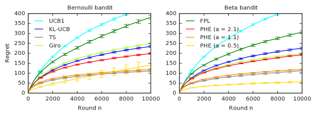
  Model Run time (seconds) $K$ $n$ ${\tt TS}$ ${\tt PHE}$ ${\tt Giro}$ $5$ $1$k $13.9$ $18.2$ $48.7$ $10$ $1$k $13.5$ $17.0$ $83.1$ $20$ $1$k $14.7$ $19.1$ $157.0$ $5$ $10$k $134.7$ $179.5$ $843.5$ $10$ $10$k $146.0$ $180.3$ $1250.2$ $20$ $10$k $136.3$ $182.6$ $1916.5$
       (a)                                              (b)                                                (c)

Figure 1: a. Comparison of ${\tt PHE}$ to multiple baselines in a Bernoulli bandit. b. Comparison of ${\tt PHE}$ to multiple baselines in a beta bandit. c. Run times of three randomized algorithms in a beta bandit. All results are averaged over $100$ randomly chosen problems.

We compare ${\tt PHE}$ to five baselines: ${\tt UCB1}$ Auer et al. (2002), ${\tt KL\mathchar 45\relax UCB}$ Garivier and Cappe (2011), Bernoulli ${\tt TS}$ Agrawal and Goyal (2013a) with a $\mathrm{Beta}(1,1)$ prior, ${\tt Giro}$ Kveton et al. (2019b), and ${\tt FPL}$ Neu and Bartok (2013). The baselines are chosen for the following reasons. ${\tt KL\mathchar 45\relax UCB}$ and ${\tt TS}$ are statistically near-optimal in Bernoulli bandits. We implement them with $[0,1]$ rewards as follows. For any observed reward $Y_{i,t}\in[0,1]$, we draw $\hat{Y}_{i,t}\sim\mathrm{Ber}(Y_{i,t})$ and then use it instead of $Y_{i,t}$ Agrawal and Goyal (2013a). ${\tt Giro}$ is chosen because it explores similarly to ${\tt PHE}$, by adding pseudo-rewards to its history (Section 6). We implement it with $a=1$, as analyzed in Kveton et al. (2019b). ${\tt FPL}$ is chosen because it perturbs the estimates of mean rewards similarly to ${\tt PHE}$ (Section 6). We implement it with geometric resampling and exponential noise, as described in Neu and Bartok (2013).

We experiment with three settings of perturbation scales $a$ in ${\tt PHE}$: $2.1$, $1.1$, and $0.5$. The first value is greater than $2$ and is formally justified in Section 4. The second value is greater than $1$ and is informally justified in Section 3. The last value is used to illustrate that the regret of ${\tt PHE}$ can be linear when ${\tt PHE}$ is not parameterized properly.

To run ${\tt PHE}$ with a non-integer perturbation scale $a$, we replace $as$ in ${\tt PHE}$ with $\left\lceil as\right\rceil$. The analysis of ${\tt PHE}$ in Section 4 can be extended to this setting. We also experimented with $a=1$ and $a=2$. We do not report these results because they are similar to those at $a=1.1$ and $a=2.1$.

5.1 Comparison to Baselines

In the first experiment, we evaluate ${\tt PHE}$ on two classes of the bandit problems in Kveton et al. (2019b). The first class is a Bernoulli bandit where $P_{i}=\mathrm{Ber}(\mu_{i})$. The second class is a beta bandit where $P_{i}=\mathrm{Beta}(v\mu_{i},v(1-\mu_{i}))$ and $v=4$. We experiment with $100$ randomly chosen problems in each class. Each problem has $K=10$ arms and the mean rewards of these arms are chosen uniformly at random from interval $[0.25,0.75]$. The horizon is $n=10000$ rounds.

Our results are reported in Figures 1a and 1b. We observe that ${\tt PHE}$ with $a>1$ outperforms four of our baselines: ${\tt UCB1}$, ${\tt KL\mathchar 45\relax UCB}$, ${\tt Giro}$, and ${\tt FPL}$. This is unexpected, since the design of ${\tt PHE}$ is conceptually simple; and neither requires nor uses confidence intervals or posteriors. ${\tt PHE}$ becomes competitive with ${\tt TS}$ at $a=1.1$. Note that the regret of ${\tt PHE}$ is linear in the Bernoulli bandit at $a=0.5$. This shows that our suggestions for setting the perturbation scale $a$ are reasonably tight.

5.2 Computational Cost

In the second experiment, we compare the run times of three randomized algorithms: ${\tt TS}$, which samples from a beta posterior; ${\tt Giro}$, which bootstraps from a history with pseudo-rewards; and ${\tt PHE}$, which samples pseudo-rewards from a binomial distribution. The number of arms is between $5$ and $20$, and the horizon is up to $n=10000$ rounds.

Our results are reported in Figure 1c. In all settings, the run time of ${\tt PHE}$ is comparable to that of ${\tt TS}$. The run time of ${\tt Giro}$ is an order of magnitude higher. The reason is that the computational cost of bootstrapping grows linearly with the number of past observations.

6 Related Work

Our algorithm design bears a similarity to three existing designs, which we discuss in detail below.

${\tt Giro}$ is a bandit algorithm where the mean reward of the arm is estimated by its average reward in a bootstrap sample of its history with pseudo-rewards Kveton et al. (2019b). The algorithm has a provably sublinear regret in a Bernoulli bandit. ${\tt PHE}$ improves over ${\tt Giro}$ in three respects. First, its design is simpler, because ${\tt PHE}$ merely adds random pseudo-rewards and does not bootstrap. Second, ${\tt PHE}$ has a sublinear regret in any $K$-armed bandit with $[0,1]$ rewards. Third, ${\tt PHE}$ is computationally efficient beyond a Bernoulli bandit. We discuss this in Section 3.

Our work is also closely related to posterior sampling. In particular, let $\mu\sim\mathcal{N}(\mu_{0},\sigma^{2})$ and $(Y_{\ell})_{\ell=1}^{s}\sim\mathcal{N}(\mu,\sigma^{2})$ be $s$ i.i.d. noisy observations of $\mu$. Then the posterior distribution of $\mu$ conditioned on $(Y_{\ell})_{\ell=1}^{s}$ is

$$\mathcal{N}\left(\frac{\mu_{0}+\sum_{\ell=1}^{s}Y_{\ell}}{s+1},\,\frac{\sigma^{2}}{s+1}\right)\,.$$ (7)

A sample from this distribution can be also drawn as follows. First, draw $s+1$ i.i.d. samples $(Z_{\ell})_{\ell=0}^{s}\sim\mathcal{N}(0,\sigma^{2})$. Then

$$\frac{\mu_{0}+\sum_{\ell=1}^{s}Y_{\ell}+\sum_{\ell=0}^{s}Z_{\ell}}{s+1}$$

is a sample from (7). Unfortunately, the above equivalence holds only for normal random variables. Therefore, it cannot justify ${\tt PHE}$ as a form of Thompson sampling. Nevertheless, the scale of the perturbation is similar to (1), which suggests that ${\tt PHE}$ is sound.

Follow the perturbed leader (FPL) Hannan (1957); Kalai and Vempala (2005) is an algorithm design where the learning agent pulls the arm with the lowest perturbed cumulative cost. In our notation, $I_{t}=\operatorname*{arg\,min\,}_{i\in[K]}\tilde{V}_{i,t-1}+\tilde{U}_{i,t}$, where $\tilde{V}_{i,t-1}$ is the cumulative cost of arm $i$ in the first $t-1$ rounds and $\tilde{U}_{i,t}$ is the perturbation of arm $i$ in round $t$. ${\tt PHE}$ differs from FPL in three respects. First, $\tilde{U}_{i,t}=O(\sqrt{n})$ in FPL. In ${\tt PHE}$, the noise in round $t$ adapts to the number of arm pulls, because $U_{i,T_{i,t-1}}=O(T_{i,t-1})$. Second, FPL has been traditionally studied in the non-stochastic full-information setting. In comparison, ${\tt PHE}$ is designed for the stochastic bandit setting. Neu and Bartok (2013) extended FPL to the bandit setting using geometric resampling and we compare to their algorithm in Section 5. Finally, all existing FPL analyses derive gap-free regret bounds. We derive a gap-dependent regret bound.

7 Conclusions

We propose a new online algorithm, ${\tt PHE}$, for cumulative regret minimization in stochastic multi-armed bandits. The key idea in ${\tt PHE}$ is to add $O(t)$ i.i.d. pseudo-rewards to the history in round $t$ and then pull the arm with the highest average reward in this perturbed history. The pseudo-rewards are drawn from the maximum variance distribution. We derive $O(K\Delta^{-1}\log n)$ and $O(\sqrt{Kn\log n})$ bounds on the $n$-round regret of ${\tt PHE}$, where $K$ is the number of arms and $\Delta$ is the minimum gap between the mean rewards of the optimal and suboptimal arms. This result is unexpected, since the design of ${\tt PHE}$ is conceptually simple. We empirically compare ${\tt PHE}$ to several baselines and show that it is competitive with the best of them.

${\tt PHE}$ can be easily adapted to any reward distributions with a bounded support. If $Y_{i,t}\in[m,M]$, $Y_{i,t}$ in line 19 of ${\tt PHE}$ should be replaced with $(Y_{i,t}-m)/(M-m)$.

${\tt PHE}$ can be applied to structured problems, such as generalized linear bandits Filippi et al. (2010), as follows. Let $x_{i}$ be the feature vector of arm $i$. Then $((x_{I_{\ell}},Y_{I_{\ell},\ell}))_{\ell=1}^{t-1}$ is the history in round $t$ and a natural choice for the pseudo-history is $((x_{I_{\ell}},Z_{j,\ell}))_{j\in[a],\,\ell\in[t-1]}$, where $Z_{j,\ell}\sim\mathrm{Ber}(1/2)$ are i.i.d. random variables. In round $t$, the learning agent fits a reward generalization model to a mixture of both histories and pulls the arm with the highest estimated reward in that model. We leave the analysis and empirical evaluation of this algorithm for future work. The algorithm was analyzed in a linear bandit in Kveton et al. (2019a).

We believe that ${\tt PHE}$ can be extended to other perturbation schemes. For instance, since $\mathrm{var}\left[V_{i,s}\right]\leq s/4$, it is plausible that any $s$ i.i.d. pseudo-rewards with a comparable variance, such as $(Z_{\ell})_{\ell=1}^{s}\sim\mathcal{N}(0,1/4)$, would lead to optimism. We leave the analyses of such designs for future work.

Appendix A Technical Lemmas

Fix arm $i$ and the number of its pulls $n$. Let $X$ be the cumulative reward of arm $i$ after $n$ pulls and $Y=\sum_{\ell=1}^{2an}Z_{\ell}$ be the sum of $2an$ i.i.d. pseudo-rewards $(Z_{\ell})_{\ell=1}^{2an}\sim\mathrm{Ber}(1/2)$. Note that both $X$ and $Y$ are random variables. Let $\bar{X}=\mathbb{E}\left[X\right]$ and $\bar{Y}=\mathbb{E}\left[Y\right]$. Our main theorem is stated and proved below.

Theorem 4.

For any $a>1$,

$$\mathbb{E}\left[1/\mathbb{P}\left(X+Y\geq\bar{X}+\bar{Y}\,\middle|\,X\right)\right]$$

$$\quad\leq\frac{2e^{2}\sqrt{a}}{\sqrt{\pi}}\exp\left[\frac{8}{a-1}\right]\left(1+\sqrt{\frac{\pi a}{8(a-1)}}\right)\,.$$

Proof.

Let $W=\mathbb{E}\left[1/\mathbb{P}\left(Y\geq\bar{X}-X+\bar{Y}\,\middle|\,X\right)\right]$. Note that $W$ can be rewritten as $W=\mathbb{E}\left[f(X)\right]$, where

$$f(X)=\left[\smashoperator[r]{\sum_{y=\left\lceil\bar{X}-X+an\right\rceil}^{m}}B(y;m,1/2)\right]^{-1}$$

and $m=2an$. This follows from the definition of $Y$ and that $\bar{Y}=an$.

Note that $f(X)$ decreases in $X$, as required by Lemma 1, because the probability of observing at least $\left\lceil\bar{X}-X+an\right\rceil$ ones increases with $X$ and $f(X)$ is its reciprocal. So we can apply Lemma 1 and get

$$W\leq{} \sum_{i=0}^{i_{0}-1}\exp[-2i^{2}]\left[\smashoperator[r]{\sum_{y=\left\lceil an+(i+1)\sqrt{n}\right\rceil}^{m}}B(y;m,1/2)\right]^{-1}+{}$$

$$\exp[-2i_{0}^{2}]\left[\smashoperator[r]{\sum_{y=\left\lceil an+\bar{X}\right\rceil}^{m}}B(y;m,1/2)\right]^{-1}\,,$$

where $i_{0}$ is the smallest integer such that $(i_{0}+1)\sqrt{n}\geq\bar{X}$, as defined in Lemma 1.

Now we bound the sums in the reciprocals from below using Lemma 2. For $\delta=(i+1)\sqrt{n}$,

$$\smashoperator[r]{\sum_{y=\left\lceil an+(i+1)\sqrt{n}\right\rceil}^{m}}B(y;m,1/2)\geq\frac{\sqrt{\pi}}{e^{2}\sqrt{a}}\exp\left[-\frac{2(i+2)^{2}}{a}\right]\,.$$

For $\delta=\bar{X}$,

$$\smashoperator[r]{\sum_{y=\left\lceil an+\bar{X}\right\rceil}^{m}}B(y;m,1/2) \geq\frac{\sqrt{\pi}}{e^{2}\sqrt{a}}\exp\left[-\frac{2(\bar{X}+\sqrt{n})^{2}}{an}\right]$$

$$\geq\frac{\sqrt{\pi}}{e^{2}\sqrt{a}}\exp\left[-\frac{2(i_{0}+2)^{2}}{a}\right]\,,$$

where the last inequality is from the definition of $i_{0}$. Then we chain the above three inequalities and get

$$W\leq\frac{e^{2}\sqrt{a}}{\sqrt{\pi}}\sum_{i=0}^{i_{0}}\exp\left[-\frac{2ai^{2}-2(i+2)^{2}}{a}\right]\,.$$

Now note that

$$2ai^{2}-2(i+2)^{2}$$

$$\quad=2(a-1)i^{2}-8i-8$$

$$\quad=2(a-1)\left(i^{2}-\frac{4i}{a-1}+\frac{4}{(a-1)^{2}}-\frac{4}{(a-1)^{2}}\right)-8$$

$$\quad=2(a-1)\left(i-\frac{2}{a-1}\right)^{2}-\frac{8a}{a-1}\,.$$

It follows that

$$W \leq\frac{e^{2}\sqrt{a}}{\sqrt{\pi}}\sum_{i=0}^{i_{0}}\exp\left[-\frac{2(a-1)}{a}\left(i-\frac{2}{a-1}\right)^{2}+\frac{8}{a-1}\right]$$

$$\leq\frac{2e^{2}\sqrt{a}}{\sqrt{\pi}}\exp\left[\frac{8}{a-1}\right]\sum_{i=0}^{\infty}\exp\left[-\frac{2(a-1)}{a}i^{2}\right]$$

$$\leq\frac{2e^{2}\sqrt{a}}{\sqrt{\pi}}\exp\left[\frac{8}{a-1}\right]\!\left[1+\!\!\!\smashoperator[r]{\int_{u=0}^{\infty}}\exp\left[-\frac{2(a-1)}{a}u^{2}\right]\mathop{}\!\mathrm{d}u\right]$$

$$=\frac{2e^{2}\sqrt{a}}{\sqrt{\pi}}\exp\left[\frac{8}{a-1}\right]\left(1+\sqrt{\frac{\pi a}{8(a-1)}}\right)\,.$$

This concludes our proof.  

Lemma 1.

Let $f(X)$ be a non-negative decreasing function of random variable $X$ in Theorem 4 and $i_{0}$ be the smallest integer such that $(i_{0}+1)\sqrt{n}\geq\bar{X}$. Then

$$\mathbb{E}\left[f(X)\right]\leq{} \sum_{i=0}^{i_{0}-1}\exp[-2i^{2}]f(\bar{X}-(i+1)\sqrt{n})+{}$$

$$\exp[-2i_{0}^{2}]f(0)\,.$$

Proof.

Let

$$\mathcal{P}_{i}=\begin{cases}(\max\left\{\bar{X}-\sqrt{n},\,0\right\},\,n]\,,&i=0\,;\\ (\max\left\{\bar{X}-(i+1)\sqrt{n},\,0\right\},\,\bar{X}-i\sqrt{n}]\,,&i>0\,;\end{cases}$$

for $i\in[i_{0}]\cup\left\{0\right\}$. Then $\left\{\mathcal{P}_{i}\right\}_{i=0}^{i_{0}}$ is a partition of $[0,n]$. Based on this observation,

$$\mathbb{E}\left[f(X)\right]={} \sum_{i=0}^{i_{0}}\mathbb{E}\left[\mathds{1}\!\left\{X\in\mathcal{P}_{i}\right\}f(X)\right]$$

$$\leq{} \sum_{i=0}^{i_{0}-1}f(\bar{X}-(i+1)\sqrt{n})\,\mathbb{P}\left(X\in\mathcal{P}_{i}\right)+{}$$

$$f(0)\,\mathbb{P}\left(X\in\mathcal{P}_{i_{0}}\right)\,,$$

where the inequality holds because $f(x)$ is a decreasing function of $x$. Now fix $i>0$. Then from the definition of $\mathcal{P}_{i}$ and Hoeffding’s inequality, we have

$$\mathbb{P}\left(X\in\mathcal{P}_{i}\right)\leq\mathbb{P}\left(X\leq\bar{X}-i\sqrt{n}\right)\leq\exp[-2i^{2}]\,.$$

Trivially, $\mathbb{P}\left(X\in\mathcal{P}_{0}\right)\leq 1=\exp[-2\cdot 0^{2}]$. Finally, we chain all inequalities and get our claim.  

Lemma 2.

Let $m=2an$. Then for any $\delta\in[0,an]$,

$$\smashoperator[r]{\sum_{y=\left\lceil an+\delta\right\rceil}^{m}}B(y;m,1/2)\geq\frac{\sqrt{\pi}}{e^{2}\sqrt{a}}\exp\left[-\frac{2(\delta+\sqrt{n})^{2}}{an}\right]\,.$$

Proof.

By Lemma 4 in Appendix of Kveton et al. (2019b),

$$B(y;m,1/2)\geq\frac{\sqrt{2\pi}}{e^{2}}\sqrt{\frac{m}{y(m-y)}}\exp\left[-\frac{2(y-an)^{2}}{an}\right]\,.$$

Also note that

$$\frac{y(m-y)}{m}\leq\frac{1}{m}\frac{m^{2}}{4}=\frac{an}{2}$$

for any $y\in[0,m]$. Now we combine the above two inequalities and get

$$B(y;m,1/2)\geq\frac{2\sqrt{\pi}}{e^{2}\sqrt{an}}\exp\left[-\frac{2(y-an)^{2}}{an}\right]\,.$$

Finally, we note the following. First, the above lower bound decreases in $y$ for $y\geq an+\delta$, since $\delta\geq 0$. Second, by the pigeonhole principle, there are at least $\left\lfloor\sqrt{n}\right\rfloor$ integers between $an+\delta$ and $an+\delta+\sqrt{n}$, starting with $\left\lceil an+\delta\right\rceil$. This leads to the following lower bound

$$\smashoperator[r]{\sum_{y=\left\lceil an+\delta\right\rceil}^{m}}B(y;m,1/2) \geq\left\lfloor\sqrt{n}\right\rfloor\frac{2\sqrt{\pi}}{e^{2}\sqrt{an}}\exp\left[-\frac{2(\delta+\sqrt{n})^{2}}{an}\right]$$

$$\geq\frac{\sqrt{\pi}}{e^{2}\sqrt{a}}\exp\left[-\frac{2(\delta+\sqrt{n})^{2}}{an}\right]\,.$$

The last inequality is by $\left\lfloor\sqrt{n}\right\rfloor/\sqrt{n}\geq 1/2$, which holds for $n\geq 1$. This concludes our proof.

References

• Abbasi-Yadkori et al. [2011] Yasin Abbasi-Yadkori, David Pal, and Csaba Szepesvari. Improved algorithms for linear stochastic bandits. In Advances in Neural Information Processing Systems 24, pages 2312–2320, 2011.
• Abeille and Lazaric [2017] Marc Abeille and Alessandro Lazaric. Linear Thompson sampling revisited. In Proceedings of the 20th International Conference on Artificial Intelligence and Statistics, 2017.
• Agrawal and Goyal [2013a] Shipra Agrawal and Navin Goyal. Further optimal regret bounds for Thompson sampling. In Proceedings of the 16th International Conference on Artificial Intelligence and Statistics, pages 99–107, 2013.
• Agrawal and Goyal [2013b] Shipra Agrawal and Navin Goyal. Thompson sampling for contextual bandits with linear payoffs. In Proceedings of the 30th International Conference on Machine Learning, pages 127–135, 2013.
• Auer et al. [2002] Peter Auer, Nicolo Cesa-Bianchi, and Paul Fischer. Finite-time analysis of the multiarmed bandit problem. Machine Learning, 47:235–256, 2002.
• Chapelle and Zhang [2009] Olivier Chapelle and Ya Zhang. A dynamic Bayesian network click model for web search ranking. In Proceedings of the 18th International Conference on World Wide Web, pages 1–10, 2009.
• Dani et al. [2008] Varsha Dani, Thomas Hayes, and Sham Kakade. Stochastic linear optimization under bandit feedback. In Proceedings of the 21st Annual Conference on Learning Theory, pages 355–366, 2008.
• Filippi et al. [2010] Sarah Filippi, Olivier Cappe, Aurelien Garivier, and Csaba Szepesvari. Parametric bandits: The generalized linear case. In Advances in Neural Information Processing Systems 23, pages 586–594, 2010.
• Garivier and Cappe [2011] Aurelien Garivier and Olivier Cappe. The KL-UCB algorithm for bounded stochastic bandits and beyond. In Proceeding of the 24th Annual Conference on Learning Theory, pages 359–376, 2011.
• Gopalan et al. [2014] Aditya Gopalan, Shie Mannor, and Yishay Mansour. Thompson sampling for complex online problems. In Proceedings of the 31st International Conference on Machine Learning, pages 100–108, 2014.
• Hannan [1957] James Hannan. Approximation to Bayes risk in repeated play. In Contributions to the Theory of Games, volume 3, pages 97–140. Princeton University Press, Princeton, NJ, 1957.
• Jun et al. [2017] Kwang-Sung Jun, Aniruddha Bhargava, Robert Nowak, and Rebecca Willett. Scalable generalized linear bandits: Online computation and hashing. In Advances in Neural Information Processing Systems 30, pages 98–108, 2017.
• Kalai and Vempala [2005] Adam Kalai and Santosh Vempala. Efficient algorithms for online decision problems. Journal of Computer and System Sciences, 71(3):291–307, 2005.
• Katariya et al. [2016] Sumeet Katariya, Branislav Kveton, Csaba Szepesvari, and Zheng Wen. DCM bandits: Learning to rank with multiple clicks. In Proceedings of the 33rd International Conference on Machine Learning, pages 1215–1224, 2016.
• Kawale et al. [2015] Jaya Kawale, Hung Bui, Branislav Kveton, Long Tran-Thanh, and Sanjay Chawla. Efficient Thompson sampling for online matrix-factorization recommendation. In Advances in Neural Information Processing Systems 28, pages 1297–1305, 2015.
• Kveton et al. [2015] Branislav Kveton, Csaba Szepesvari, Zheng Wen, and Azin Ashkan. Cascading bandits: Learning to rank in the cascade model. In Proceedings of the 32nd International Conference on Machine Learning, 2015.
• Kveton et al. [2019a] Branislav Kveton, Csaba Szepesvari, Mohammad Ghavamzadeh, and Craig Boutilier. Perturbed-history exploration in stochastic linear bandits. In Proceedings of the 35th Conference on Uncertainty in Artificial Intelligence, 2019.
• Kveton et al. [2019b] Branislav Kveton, Csaba Szepesvari, Sharan Vaswani, Zheng Wen, Mohammad Ghavamzadeh, and Tor Lattimore. Garbage in, reward out: Bootstrapping exploration in multi-armed bandits. In Proceedings of the 36th International Conference on Machine Learning, pages 3601–3610, 2019.
• Lai and Robbins [1985] T. L. Lai and Herbert Robbins. Asymptotically efficient adaptive allocation rules. Advances in Applied Mathematics, 6(1):4–22, 1985.
• Lattimore and Szepesvari [2019] Tor Lattimore and Csaba Szepesvari. Bandit Algorithms. Cambridge University Press, 2019.
• Li et al. [2017] Lihong Li, Yu Lu, and Dengyong Zhou. Provably optimal algorithms for generalized linear contextual bandits. In Proceedings of the 34th International Conference on Machine Learning, pages 2071–2080, 2017.
• Lipton et al. [2018] Zachary Lipton, Xiujun Li, Jianfeng Gao, Lihong Li, Faisal Ahmed, and Li Deng. BBQ-networks: Efficient exploration in deep reinforcement learning for task-oriented dialogue systems. In Proceedings of the 32nd AAAI Conference on Artificial Intelligence, pages 5237–5244, 2018.
• Liu et al. [2018] Bing Liu, Tong Yu, Ian Lane, and Ole Mengshoel. Customized nonlinear bandits for online response selection in neural conversation models. In Proceedings of the 32nd AAAI Conference on Artificial Intelligence, pages 5245–5252, 2018.
• Lu and Van Roy [2017] Xiuyuan Lu and Benjamin Van Roy. Ensemble sampling. In Advances in Neural Information Processing Systems 30, pages 3258–3266, 2017.
• Neu and Bartok [2013] Gergely Neu and Gabor Bartok. An efficient algorithm for learning with semi-bandit feedback. In Proceedings of the 24th International Conference on Algorithmic Learning Theory, pages 234–248, 2013.
• Popoviciu [1935] Tiberiu Popoviciu. Popoviciu’s inequality on variances. https://en.wikipedia.org/wiki/Popoviciu’s_inequality_on_variances, 1935.
• Radlinski et al. [2008] Filip Radlinski, Robert Kleinberg, and Thorsten Joachims. Learning diverse rankings with multi-armed bandits. In Proceedings of the 25th International Conference on Machine Learning, pages 784–791, 2008.
• Riquelme et al. [2018] Carlos Riquelme, George Tucker, and Jasper Snoek. Deep Bayesian bandits showdown: An empirical comparison of Bayesian deep networks for Thompson sampling. In Proceedings of the 6th International Conference on Learning Representations, 2018.
• Russo et al. [2018] Daniel Russo, Benjamin Van Roy, Abbas Kazerouni, Ian Osband, and Zheng Wen. A tutorial on Thompson sampling. Foundations and Trends in Machine Learning, 11(1):1–96, 2018.
• Thompson [1933] William R. Thompson. On the likelihood that one unknown probability exceeds another in view of the evidence of two samples. Biometrika, 25(3-4):285–294, 1933.
• Zhang et al. [2016] Lijun Zhang, Tianbao Yang, Rong Jin, Yichi Xiao, and Zhi-Hua Zhou. Online stochastic linear optimization under one-bit feedback. In Proceedings of the 33rd International Conference on Machine Learning, pages 392–401, 2016.