Supervised learning improves disease outbreak detection

Abstract

The early detection of infectious disease outbreaks is a crucial task to protect population health. To this end, public health surveillance systems have been established to systematically collect and analyse infectious disease data. A variety of statistical tools are available, which detect potential outbreaks as abberations from an expected endemic level using these data. Here, we develop the first supervised learning approach based on hidden Markov models for disease outbreak detection, which leverages data that is routinely collected within a public health surveillance system. We evaluate our model using real Salmonella and Campylobacter data, as well as simulations. In comparison to a state-of-the-art approach, which is applied in multiple European countries including Germany, our proposed model reduces the false positive rate by up to 50% while retaining the same sensitivity. We see our supervised learning approach as a significant step to further develop machine learning applications for disease outbreak detection, which will be instrumental to improve public health surveillance systems.

1 Introduction

Infectious diseases are a significant threat to human health. In order to guard against these infections, public health surveillance systems have been established to systematically collect, analyse and interpret data to guide public health actions [1]. A central part of public health surveillance is the early detection of disease outbreaks. In Germany, data about notifiable infectious diseases is continuously reported from local and federal health authorities to the Robert Koch Institute (RKI) and collected using an electronic surveillance system (SurvNet) for infectious disease outbreaks, which was established in 2001 [2]. Thousands of time series of case counts from the SurvNet database are analysed each week to detect aberrations (i.e. potential outbreaks) from an expected endemic baseline. A plethora of methods are available to accomplish this task, most of which use either regression techniques or statistical process control (e.g. [3, 4, 5, 6, 7]). An excellent review of methods can be found in [8].
The Farrington algorithm is a popular method for disease outbreak detection, which has been used in multiple European countries [9, 4]. The RKI uses an improved version, which is implemented as ’farringtonFlexible’ (FF) in the R package surveillance [10, 11, 6]. In brief, the algorithm fits a quasi-Poisson Generalized Linear Model (GLM) of the endemic baseline (i.e. no outbreaks) on past data, accounting for possible time trends and seasonal patterns. During model fitting the most recent weeks (default: 26) are excluded to avoid an influence of recent outbreaks. Then the model predicts the endemic baseline for the current week and calculates an alarm threshold either based on the prediction interval or a quantile of the Negative Binomial distribution. If the number of cases in the current week exceeds the alarm threshold, a report is created for further investigation. One crucial factor of this process is a proper balancing between the sensitivity and the false positive rate of the generated alarms. It is important that the recipients of the alarm reports are not overwhelmed by too many false alarms, but at the same time, sensitivity has to be high enough to capture relevant signals. The FF algorithm has proven to be a good choice to accomplish this task at the RKI. In a systematic evaluation of 19 available methods using simulations it had the lowest false positive rate, while retaining a reasonable sensitivitiy [12]. However, this algorithm still generates many false alarms in practice that have to be verified by epidemiologists, which costs time and money.
Outbreaks that are detected and confirmed e.g. by local health authorities or the RKI, are also recorded in the SurvNet database. In this work, we consider outbreaks that are defined according to the Protection against Infection Act which determines compulsory registration of ’suspicion and disease of microbial foodborne disease or acute gastroenteritis if two or more diseases of similar type occur, in which an epidemic connection is probable or suspected’ [13]. The reported outbreaks contain information about cases, including the dates of infection and location, which is available on the level of counties. From this data we generate time series for counties of weekly case counts and class labels indicating whether an outbreak occured or not. Our proposed supervised learning approach is trained on this data to classify weeks into an endemic (baseline) or outbreak state by exploiting the fact that weeks with reported outbreaks exhibit an excess number of cases compared to weeks where no outbreak was reported. The approach is based on hidden Markov models (HMMs), which have been used successfully in many machine learning applications for analysis of sequential data, such as speech recognition or genome analysis (e.g. [14, 15]).
The main goal of this study is to improve the prospective detection of potential infectious disease outbreaks. In particular, we aim at a reduction of false alarms - while maintaining sensitivity of state-of-the-art methods - which will save valuable time during verification of the generated alarm reports. We compare our proposed method to the FF algorithm on simulations and real data of Salmonella and Campylobacter infections and show that our approach reduces the false positive rate by up to 50% at the same sensitivity.

2 Methods

We assume that our data are governed by a HMM. We specify our model using a set of $N$ time series to make use of the outbreak labels from multiple time series during model training, i.e. at any time point $t\in\left[1;T\right]$ in time series $n\in\left[1;N\right]$, the corresponding obervation $o_{n,t}$ is emitted from a hidden state $s_{n,t}\in\mathcal{K}$ that evolves over time according to a first-order Markov process. Thus a HMM with a set of states $\mathcal{K}$ has the following components:

• $\mathcal{O}=\left\{O_{1},\ldots,O_{N}\right\}$ the sequences of observations, where $O_{n}=(o_{n,1},\ldots,o_{n,T})$

• $\mathcal{S}=\left\{S_{1},\ldots,S_{N}\right\}$ the sequences of latent underlying states, where $S_{n}=(s_{n,1},\ldots,s_{n,T})$ and $s_{n,t}\in\mathcal{K}$

• $Z=\left(z_{1},\ldots,z_{T}\right)$ a sequence of covariates for each time point

• $\pi_{i}=\Pr(s_{n,1}=i\bigr{)}$ the vector of initial state probabilities, where $\sum_{j\in\mathcal{K}}\Pr(s_{n,1}=j\bigr{)}=1$

• $a_{ij}=\Pr\left(s_{n,t}=j\left|s_{n,t-1}=i\right.\right)$ transition probabilities between the states $i,j\in\mathcal{K}$,
  i.e. $\sum_{j\in\mathcal{K}}\Pr\left(s_{n,t+1}=j|s_{n,t}=i\right)=1$

• $\psi_{s_{n,t}}\left(o_{n,t}\left|z_{t}\right.\right)$ is a vector of emission functions $\psi_{s_{n,t}}\left(o_{n,t}\left|z_{t}\right.\right)=\Pr\left(o_{n,t}\left|s_{n,t},z_{t}\right.\right)$ that provides the components of the mixture distribution, i.e. the conditional densitites of $o_{n,t}$ associated with state $s_{n,t}$, at time $t$ in time series $n$ and covariate $z_{t}$

• Parameter vector $\theta=\left(\pi_{i},a_{ij},\psi\right)$ specifies the HMM

In surveillance data, the observations are the reported number of cases of a certain disease during a certain time, e.g. weeks. In our setting, we are interested in $\mathcal{\left|K\right|}=2$ hidden states, i.e. $s_{n,t}\in\{0,1\}$, where $s_{n,t}=1$ indicates an ongoing outbreak with an excess number of cases at week $t$, and $s_{n,t}=0$ applies to weeks where the case number is consistent with the expected baseline (endemic). As many infectious diseases and hence the corresponding surveillance data follow an annual pattern or time trend, a natural choice for $Z$ is the sequence $z_{t}=\left(t,\cos\left(\frac{2\pi}{52}t\right),\sin\left(\frac{2\pi}{52}t\right)\right)$ to model secular and seasonal trends. We assume that the data in our surveillance time series follows a negative Binomial distribution: $o_{n,t}\sim\text{$\mathcal{NB}$}(\mu_{n,t},r_{n})$, where $r_{n}$ is the size parameter of the negative Binomial distribution and

$$\log\mu_{n,t}=\beta_{n,0}+\beta_{n,1}t+\beta_{n,2}\cos\left(\frac{2\pi}{52}t\right)+\beta_{n,3}\sin\left(\frac{2\pi}{52}t\right)+\beta_{4}s_{n,t}$$

the $\log$ of the the expected number of cases $\mu_{n,t}$ in time series $n$ at time $t$. Here, $\beta_{n,0}$ is the baseline number of cases, $\beta_{n,1}$ a secular time trend and $\beta_{n,3}$ and $\beta_{n,4}$ describe seasonal patterns for each time series $n\in\left[1;N\right]$. The state-dependence of $o_{n,t}$ on $s_{n,t}$ - and thus the effect of an outbreak - is incoporated by a multiplicative factor $\exp\left(\beta_{4}\right)$ that describes the excess number of cases in outbreak situations. Note that, while $\beta_{n,0},\beta_{n,1},\beta_{n,2},\beta_{n,3}$ are specific for each time series, $\beta_{4}$ is the same for all. This allows that information about past outbreaks is shared across time series. This is necessary to make the model robust, since the number of outbreaks can vary greatly between time series. If only a few outbreaks occured in the training data of a single time series, fitting a model with a specific parameter for the effect of an outbreak would not generalize well on new data. In particular, it would not be possible to fit a model on a single time series if there is no outbreak in the past training data.

Parameter learning.

Since there is a reporting delay of outbreaks - i.e. outbreaks in the recent past are not yet recorded in SurvNet - we exclude $u$ time units from our training data: $T_{train}=T-u$. Assuming independence between individual time series, the likelihood of our model with known state sequences $S_{n}^{train}=\left(s_{n,1},\ldots,s_{n,T_{train}}\right)\in\mathcal{S}_{train}$ and observation sequences $O_{n}^{train}=\left(o_{n,1},\ldots,o_{n,T_{train}}\right)\in\mathcal{O}_{train}$ is:

$$\mbox{Pr}(\mathcal{O}_{train},\mathcal{S}_{train}\left|\theta,Z\right.) =\prod_{n=1}^{N}\mbox{Pr}(O_{n}^{train}\mid S_{n}^{train},Z,\theta)\cdot\mbox{Pr}(S_{n}^{train}\left|\theta\right.)$$

$$=\prod_{n=1}^{N}\left[\prod_{t=1}^{T_{train}}\psi_{s_{n,t}}(o_{n,t}\left|z_{t}\right.)\cdot\prod_{t=2}^{T_{train}}a_{s_{n,t-1}s_{n,t}}\cdot\pi_{s_{n,1}}\right]$$

Maximum likelihood estimation of model parameters $\pi_{i}$ and $a_{i,j}$ is straightforward:

$$a_{i,j} =\frac{\sum_{n=1}^{N}\sum_{t=2}^{T_{train}}\delta\left(s_{n,t-1},i\right)\delta\left(s_{n,t},j\right)}{\sum_{n=1}^{N}\sum_{t=2}^{T_{train}}\delta\left(s_{n,t-1},i\right)}$$

$$\pi_{i} =\frac{\sum_{n=1}^{N}\delta\left(s_{1},i\right)}{N}$$

where $\delta(i,j)=\left\{\begin{tabular}[]{l}1, if i = j\\ 0, if i $\neq$ j\end{tabular}\right.$. Estimation of $\beta=\left(\beta_{n,0},\beta_{n,1},\beta_{n,2},\beta_{n,3},\beta_{4}\right)$ is carried out using the Iteratively Reweighted Least Squares algorithm for Generalized Linear Models, for which the R functions glm.fit() and glm.nb() are used [16, 17].

Posterior probability of an outbreak.

In order to determine whether time point $T$ in time series $n$ is in the endemic or in the outbreak state, the posterior probability

$$\Pr\left(s_{n,T}=1\left|O_{n},\theta\right.\right)=\frac{\Pr\left(s_{n,T}=1,O_{n}\left|\theta\right.\right)}{\sum_{s_{n,T\in\left\{0,1\right\}}}\Pr\left(s_{n,T},O_{n}\left|\theta\right.\right)}$$

is calculated. This can be done efficiently using recursive computation of the forward probabilites $\alpha_{n,t}\left(i\right)=\Pr\left(s_{n,t}=i,O_{n}\left|\theta\right.\right)$ of a HMM [15].

Data and model fitting.

Time series data were extracted for Salmonella and Campylobacter infections from the SurvNet database (accessible online: https://survstat.rki.de/), which collects reports about notifiable diseases at the RKI. Data were aggregated by disease, local health authorities - representing counties or districts in Germany - and weeks. Weekly outbreak labels were assigned to counties if at least two cases were part of an outbreak in that week. For a further description of the outbreak data and labels see [18]. Time series were randomly assigned to 20 equally sized groups, ensuring that each group had enough outbreaks for training. For each week in 2010-2017 models were trained on data using the past five years excluding the latest 26 weeks.

Simulations.

To assess model performance in a controlled setting, we adapted 14 different simulation scenarios as proposed in Noufaily et al. [6]. In short, expected case counts for each time series with a length of 624 were simulated from a linear model including Fourier terms for an annual seasonal pattern and an optional time trend: $\mu_{t}=\exp\left(\beta_{0}+\beta_{1}t+\beta_{2}\cos\left(\frac{2\pi}{52}t\right)+\beta_{3}\sin\left(\frac{2\pi}{52}t\right)\right)$. Parameters for all simulation scenarios are depicted in Supplementary Table 1. The state sequences of endemic and outbreak weeks were simulated using a transition matrix, where for each time series, $a_{00}$ was sampled from a uniform distribution from the interval $\left[0.9;1\right]$ and $a_{11}$ was sampled from $\left[0.4;0.6\right]$. As an additional parameter, each scenario is assigned a dispersion parameter $\phi\geq 1$ (Supplementary Table 1). Weekly case counts of the endemic state were then sampled from a Negative Binomial with mean $\mu_{t}$ and variance $\phi\mu_{t}$. For time points in the outbreak state, $\mu_{t}$ was chosen such that the power of detecting the outbreak with a p-value < 0.01 from the endemic distribution was 0.5.

Evaluation and benchmarking.

Performance of the HMM was compared to the FF algorithm, which is currently the method of choice for outbreak detection at the RKI. The farringtonFlexible() function from the R package surveillance was used with the following (default) control parameters: noPeriods = 10, b = 5, w = 3, weightsThreshold = 2.58, pastWeeksNotIncluded = 26, thresholdMethod = "nbPlugin", alpha = 0.01 [11]. ROC curves, sensitivity, false positive rate and precision were computed using the R package ROCR [19].

Availability.

The R source code of the model is part of this paper as Supplementary Information.

3 Results

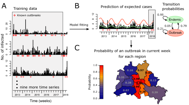
Figure 1: Overview of the method using simulated data for twelve districts in Berlin. For reasons of data protection, outbreak data cannot be shown for individual counties. To get a realistic sceanrio for illustration of the method, the data was simulated from HMMs which were fit to real data of Salmonella infections. (A) The example shows five years of data of simulated Salmonella infections in Berlin. The hidden Markov model is trained on reported cases and outbreaks, indicated by the shaded area. (B) The expected number of cases in the endemic (green) and the outbreak (red) state are shown, which are extrapolated up to the current week (dashed lines). The fitted transition proababilities are shown as a graph. (C) For each region, the posterior probabilities are calculated.

We briefly want to illustrate the workflow and components of our method with an application to a set of infectious disease surveilance data using a simulated example of the twelve districts of Berlin (Figure 1). By default the HMM uses five years of training data for outbreak detection in the current week, however other durations are possible. The past 26 weeks are excluded from the training data to avoid model training on incomplete data due to possible reporting delays. Since the frequency of disease outbreaks varies between counties, one model is trained on multiple time series (in our example one model is trained for the 12 districts of Berlin) to make sure that enough past outbreaks are available for training (Figure 1A). The fitted HMM consists of a linear predictor, initial state and transition probabilities (Figure 2B). Using the generalized linear model, the expected number of cases of the endemic and the outbreak state is predicted for the current week. Then the probability of an outbreak in the current week is calculated for all time series, which is depicted on a map in our example (Figure 3C). An alarm will be triggered, if the probability exceeds a chosen threshold.
We applied the HMM and the FF algorithm to Salmonella and Campylobacter cases reported from more than 400 counties in Germany and simulated data (Methods). Figure 2 shows Salmonella and Campylobacter data aggregated by week for Germany. The number of infections and outbreaks per week in Germany show a strong seasonal pattern and there is a decrease of Salmonella cases and a low increase of Campylobacter cases over time. This justifies the choice of our model to include seasonal and secular trends. We applied the models to predict outbreaks from 2010 to 2017. During this time there were 2126 Salmonanella outbreaks (according to our definiton, see Methods) with a duration of 1-8 weeks and 2260 Campylobacter outbreaks with a duration of 1-16 weeks. The average number of cases in counties which reported an outbreak in a week exhibits a marked increase compared to the average cases reported by counties where no outbreak occured in that week. This shows that weekly case counts of reported outbreaks are well separated from endemic weeks and therefore might be a valuable source of information to improve outbreak detection.
In all our applications the HMM consistently outperformed the FarringtonFlexible algorithm (Figure 3). At the same sensititvity the HMM had a lower false positive rate and a higher precision than the FF algorithm. To further investigate the different performances we set alarms with the FF algorithm using the ’nbPlugin’ threshold with $\alpha=0.01$, which are the default settings currently used at the RKI (Figure 3 A,B,C). Further, we chose the cutoff for the posterior probability of an outbreak such that the sensitivity was the same as for FF. This resulted in a sensitivity of 0.27 for simulated, 0.21 for Salmonella and 0.07 for Campylobacter data. At the same sensitivtiy, the false positive rate (fpr) for the HMM (0.0016) was roughly 50% lower than for FarringtonFlexible (0.0034), and the precision increased from 0.86 (FF) to 0.93 (HMM) on simulated data. On Salmonella data the fpr was 0.0074 for HMM, 0.0085 for FF and precisions amounted to 0.50 and 0.46 respectively. On the Campylobacter data, fpr was reduced roughly by 40% (HMM: 0.0053, FF: 0.009) and precision increased from 0.14 (FF) to 0.21 (HMM).
Furthermore, we investigated the distribution of posterior probabilities of the outbreak state in endemic weeks and weeks with reported outbreaks (Figure 3 G,H,I). There is a strong increase in posterior probabilities in outbreak weeks compared to endemic weeks in all scenarios. Moreover the posterior probability of an outbreak also increased with the size of reported outbreaks. Posterior probabilites in reported outbreak weeks were generally higher for Salmonella than Campylobacter data. This matches the fitted outbreak effects ($\exp\left(\beta_{4}\right)$, see Methods) of our HMMs. The average increase in the number of cases during an outbreak ranged from 1,7 - 8,3 fold (mean: 3.6) for Salmonella and 1,3 - 2,8 fold (mean: 1,8) for Campylobacter.
We also calculated absolute numbers of alarms and their overlap between methods and with reported outbreaks from the SurvNet database (Figure 3 J,K,L). Despite a significant overlap of correctly recalled outbreak weeks for both methods across the three applications, there is a varying amount of outbreak weeks that are exclusively recalled by one of the methods. For instance for Campylobacter, 190 reported outbreaks are recalled by each method. However, among those each method identifies 81 outbreaks that are not detected by the respective other approach.

4 Discussion

We introduced a supervised learning approach using hidden Markov models, which significantly improved performance of outbreak detection on simulated data, and real Salmonella and Campylobacter data. In our comparison with the FF algorithm, we showed that the HMM produced significantly less false alarms. Thus the application of our method in practice could reduce the workload of epidemiologists and save time and money. To the best of our knowledge, this is the first study that leverages data of past reported outbreaks from a surveillance system for their prospective detection.
The use of HMMs for modeling of epidemiological time series was also proposed in previous studies [20, 21, 22, 23, 24]. However, these were focused on the unsupervised segmentation of infectious disease data. The unsupervised HMMs showed good performance e.g. in the segmentation of Influenza cases lacking covariates for seasonal and periodic patterns. However, when using unsupervised HMMs with periodic and seasonal terms as proposed in [20] for the Campylbacter and Salmonella data, they did not perform as well as the FF algorithm. Thus we did not include them in the performance evaluation of this work.
It is also important do discuss some limitations of our approach. One obvious caveat of any supervised learning approach is, that outbreak labels are needed for model training. This data might not be available in other surveillance systems or might not be collected for all diseases of interest. In such cases one could either try to label time series afterwards or resort to other well established algorithms such as the FF algorithm.
The performance of a supervised learning approach for outbreak detection also depends on the quality of the outbreak labels. Our model exploits the fact that outbreak weeks have a higher average number of cases than endemic weeks. However, weeks with an excess number of cases are not reported (and labeled) as outbreaks if the compulsory registration criteria defined in the Protection against Infection Act are not met. This is not problematic for our approach as long as reported outbreak weeks show an increased average number of cases, separating outbreak from endemic weeks. This is the case for average case counts aggregated for weekly endemic and epidemic weeks for Germany (Figure 2). It is also verified by the fitted models, since the ’outbreak effect’ parameters $\exp\left(\beta_{4}\right)$ show a strong average increase in the number of cases in outbreak weeks. Another issue might be that smaller outbreaks are easily overlooked and thus not labeled. Apparently, small outbreaks are not very well distinguished from the endemic level, which is supported by the correlation between outbreak size and the assigned probability of an outbreak by the HMM (Figure 3 G,H,I). 73% (n=1915) of Salmonella and 83% (n=2271) of Campylobacter outbreak weeks exhibit outbreaks with only 2 or 3 cases. This also explains the low sensitivity of both methods, especially for the Campylobacter data set. Thus unlabeled small outbreaks are not problematic for our approach since they are not well distinguished from the endemic level. Ultimately the use of outbreak labels as defined in this study is justified by the significant improvement in the practical application to Salmonella and Campylobacter data.
Another limitation is that the assumption of (conditional) independence of observed time points in modeling infectious disease surveillance data is questionable, since the number of infections from one week might affect the next week. Although our proposed HMM does not take into account the dependence of subsequent observations, it incorporates dependence of the state of a current week (outbreak or endemic) on the previous week.
Future efforts will be needed to prove application of our proposed approach in daily practice of infectious disease surveillance. However, our results are promising that leveraging outbreak data with supervised learning will improve disease outbreak detection. Thus we foresee our approach to be instrumental to improve public health surveillance systems in the future.

Author Contributions

BZ initiated the study, developed the method, carried out all analyses and wrote the manuscript. IC contributed to method development and writing of the manuscript. Both authors read an approved the final version of the manuscript.

Conflict of interest

The authors declare that they have no conflict of interest.

Figures

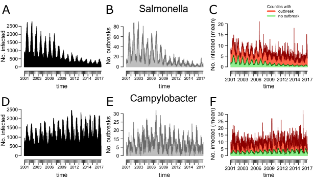
Figure 2: Aggregated weekly data of Salmonella and Campylobacter infections in Germany reported to the Robert Koch Institute. (A) The number of Salmonella infections and (B) the number of counties with a reported Salmonella outbreak show a seasonal and secular pattern. (C) The mean number of cases in counties with a reported Salmonella outbreak (red) is higher than the mean number of cases in counties without outbreak (green). (D-F) The same as (A-C) for Campylobacter infections.

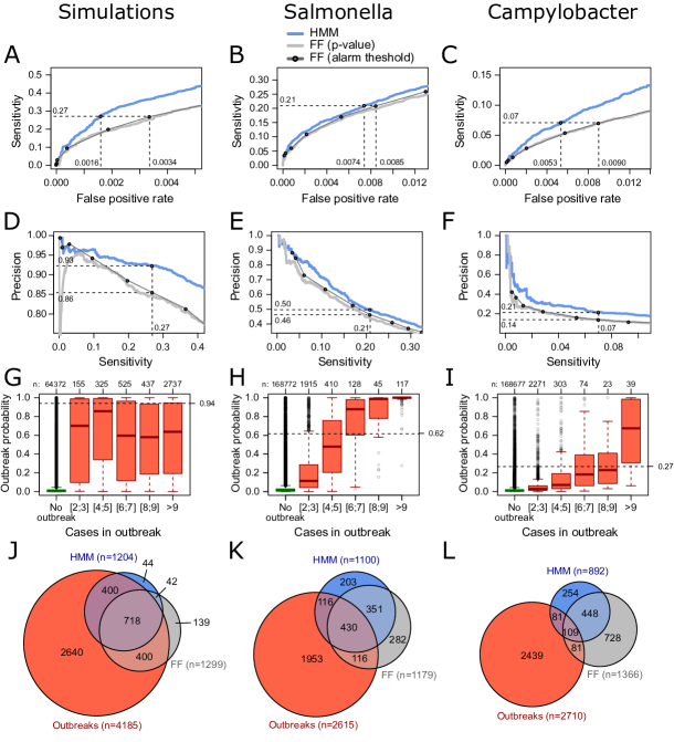
Figure 3: Results of the hidden Markov model (HMM) and the FarringtonFlexible (FF) algorithm are shown for simulations (A,D,G,J), Salmonella (B,E,H,K) and Campylobacter (C,F,I,L). Models were applied to data aggregated by county and week from 2010-2017 for Salmonella and Campylobacter. (A,B,C) False postive rate is plotted against sensitivity for posterior probability of the outbreak state (HMM) and 1 - p-value (solid grey line) for the FF algorithm. Dashed lines and grey points show sensitivity and false positive rate with cutoffs $10^{-6}$, $10^{-5}$, $10^{-4}$, $0.001$, $0.005$, $0.01$ and $0.02$ for the FF algorithm with threshold method ’nbPlugin’. (D,E,F) Sensitivity is plotted against precision for posterior probability of the outbreak state (HMM) and 1 - p-value for the FF algorithm. Dashed lines and grey points show sensitivity and false positive rate with chosen cutoffs as in (A-C). (G,H,I) Boxplots of posterior probabilities in endemic weeks (green) and weeks with reported outbreaks (red) are shown. Outbreaks were further divided by their size (i.e. the number of cases reported in the respective outbreaks). For simulations the cases in an outbreak were chosen as the excess number of cases compared to the expected endemic level. Dashed lines indicate the cutoff for posterior probabilites. (J,K,L) Venn diagrams showing the overlap of predicted outbreak weeks of the HMM and FF algorithm with reported outbreaks.

Supplementary Information

Scenario	$\beta_{0}$	$\beta_{1}$	$\beta_{2}$	$\beta_{3}$	$\phi$
1	0.1	0	0.6	0.6	1.5
2	0.1	0.0025	0.6	0.6	1.5
3	-2	0	0.1	0.3	2
4	-2	0.005	0.1	0.3	2
5	1.5	0	0.2	-0.4	1
6	1.5	0.003	0.2	-0.4	1
7	0.5	0	0.5	0.5	5
8	0.5	0.002	0.5	0.5	5
9	2.5	0	1	0.1	3
10	2.5	0.001	1	0.1	3
11	3.75	0	0.1	-0.1	1.1
12	3.75	0.001	0.1	-0.1	1.1
13	5	0	0.05	0.01	1.2
14	5	0.0001	0.05	0.01	1.2

Table 1: Parameters for all 14 simulation scenarios are shown.

References

- [1] B. C. Choi. The past, present, and future of public health surveillance. Scientifica (Cairo), 2012:875253, 2012.
- [2] D. Faensen, H. Claus, J. Benzler, A. Ammon, T. Pfoch, T. Breuer, and G. Krause. SurvNet@RKI–a multistate electronic reporting system for communicable diseases. Euro Surveill., 11(4):100–103, 2006.
- [3] D. G. Enki, P. H. Garthwaite, C. P. Farrington, A. Noufaily, N. J. Andrews, and A. Charlett. Comparison of Statistical Algorithms for the Detection of Infectious Disease Outbreaks in Large Multiple Surveillance Systems. PLoS ONE, 11(8):e0160759, 2016.
- [4] C. P. Farrington, N. J. Andrews, A. D. Beale, and M. A. Catchpole. A statistical algorithm for the early detection of outbreaks of infectious disease. Journal of the Royal Statistical Society. Series A (Statistics in Society), 159(3):547–563, 1996.
- [5] M Höhle and M. Paul. Count data regression charts for the monitoring of surveillance time series. Computational Statistics & Data Analysis, 52(9):4357 – 4368, 2008.
- [6] A. Noufaily, D. G. Enki, C. P. Farrington, P. Garthwaite, N. Andrews, and A. Charlett. An improved algorithm for outbreak detection in multiple surveillance systems. Statistics in Medicine, 32(7):1206–1222, Mar 2013.
- [7] J. Manitz and M. Höhle. Bayesian outbreak detection algorithm for monitoring reported cases of campylobacteriosis in Germany. Biom J, 55(4):509–526, Jul 2013.
- [8] S. Unkel, C. P. Farrington, P. H. Garthwaite, C. Robertson, and N. Andrews. Statistical methods for the prospective detection of infectious disease outbreaks: a review. Journal of the Royal Statistical Society: Series A (Statistics in Society), 175(1):49–82, 2012.
- [9] A. Hulth, N. Andrews, S. Ethelberg, J. Dreesman, D. Faensen, W. van Pelt, and J. Schnitzler. Practical usage of computer-supported outbreak detection in five European countries. Euro Surveill., 15(36), Sep 2010.
- [10] M. Salmon, D. Schumacher, H. Burmann, C. Frank, H. Claus, and M. Hohle. A system for automated outbreak detection of communicable diseases in Germany. Euro Surveill., 21(13), 2016.
- [11] M. Höhle. surveillance: An r package for the monitoring of infectious diseases. Computational Statistics, 22(4):571–582, Dec 2007.
- [12] G. Bedubourg and Y. Le Strat. Evaluation and comparison of statistical methods for early temporal detection of outbreaks: A simulation-based study. PLoS ONE, 12(7):e0181227, 2017.
- [13] Gesetz zur Verhütung und Bekämpfung von Infektionskrankheiten beim Menschen, 2017. Available at http://www.gesetze-im-internet.de/ifsg/index.html.
- [14] B. Zacher, M. Michel, B. Schwalb, P. Cramer, A. Tresch, and J. Gagneur. Accurate Promoter and Enhancer Identification in 127 ENCODE and Roadmap Epigenomics Cell Types and Tissues by GenoSTAN. PLoS ONE, 12(1):e0169249, 2017.
- [15] L. R. Rabiner. A tutorial on hidden markov models and selected applications in speech recognition. Proceedings of the IEEE, 77(2):257–286, Feb 1989.
- [16] W. N. Venables and B. D. Ripley. Modern Applied Statistics with S. Springer Publishing Company, Incorporated, 2010.
- [17] R. Ihaka and R. Gentleman. R: A language for data analysis and graphics. Journal of Computational and Graphical Statistics, 5(3):299–314, 1996.
- [18] S. Ghozzi and A. Ullrich. Outbreak Data Can Be Used as Labels for Machine-Learning Approaches to Outbreak Detection. in preparation, 2019.
- [19] T. Sing, O. Sander, N. Beerenwinkel, and T. Lengauer. ROCR: visualizing classifier performance in R. Bioinformatics, 21(20):3940–3941, Oct 2005.
- [20] Y. Le Strat and F. Carrat. Monitoring epidemiologic surveillance data using hidden Markov models. Statistics in Medicine, 18(24):3463–3478, Dec 1999.
- [21] R. E. Watkins, S. Eagleson, B. Veenendaal, G. Wright, and A. J. Plant. Disease surveillance using a hidden Markov model. BMC Medical Informatics and Decision Making, 9:39, Aug 2009.
- [22] C. Pelat, I. Bonmarin, M. Ruello, A. Fouillet, C. Caserio-Schonemann, D. Levy-Bruhl, Y. Le Strat, O. Retel, B. Hubert, F. Golliot, L. King, I. Mounchetrou Njoya, C. Saura, and L. Filleul. Improving regional influenza surveillance through a combination of automated outbreak detection methods: the 2015/16 season in France. Euro Surveillance, 22(32), 08 2017.
- [23] T. M. Rath, M. Carreras, and P. Sebastiani. Automated detection of influenza epidemics with hidden markov models. In Advances in Intelligent Data Analysis V, pages 521–532, Berlin, Heidelberg, 2003. Springer Berlin Heidelberg.
- [24] M. A. Martinez-Beneito, D. Conesa, A. Lopez-Quilez, and A. Lopez-Maside. Bayesian Markov switching models for the early detection of influenza epidemics. Statistics in Medicine, 27(22):4455–4468, Sep 2008.