A Multi-Domain Feature Learning Method for Visual Place Recognition

Abstract

Visual Place Recognition (VPR) is an important component in both computer vision and robotics applications, thanks to its ability to determine whether a place has been visited and where specifically. A major challenge in VPR is to handle changes of environmental conditions including weather, season and illumination. Most VPR methods try to improve the place recognition performance by ignoring the environmental factors, leading to decreased accuracy decreases when environmental conditions change significantly, such as day versus night. To this end, we propose an end-to-end conditional visual place recognition method. Specifically, we introduce the multi-domain feature learning method (MDFL) to capture multiple attribute-descriptions for a given place, and then use a feature detaching module to separate the environmental condition-related features from those that are not. The only label required within this feature learning pipeline is the environmental condition. Evaluation of the proposed method is conducted on the multi-season NORDLAND dataset, and the multi-weather GTAV dataset. Experimental results show that our method improves the feature robustness against variant environmental conditions.

I Introduction

In the last decade, the robotics community has achieved numerous breakthroughs in vision-based simultaneous localization and mapping (SLAM) [17] that have enhanced the navigation abilities of unmanned ground vehicles (UGV) and unmanned aerial vehicles (UAV) in complex environment. Visual place recognition (VPR) [7] or loop closure detection (LCD) helps robots to find loop closure in SLAM framework and is an essential element for accurate mapping and localization. Although many methods have been proposed in recent years, VPR is still a challenging problem under varying environmental conditions. Traditional VPR approaches that use handcrafted features to learn place descriptors for local scene description, often fail to extract valid features when encountering significant changes [9] in environmental conditions, such as changes in season, weather, illumination, as well as viewpoints.

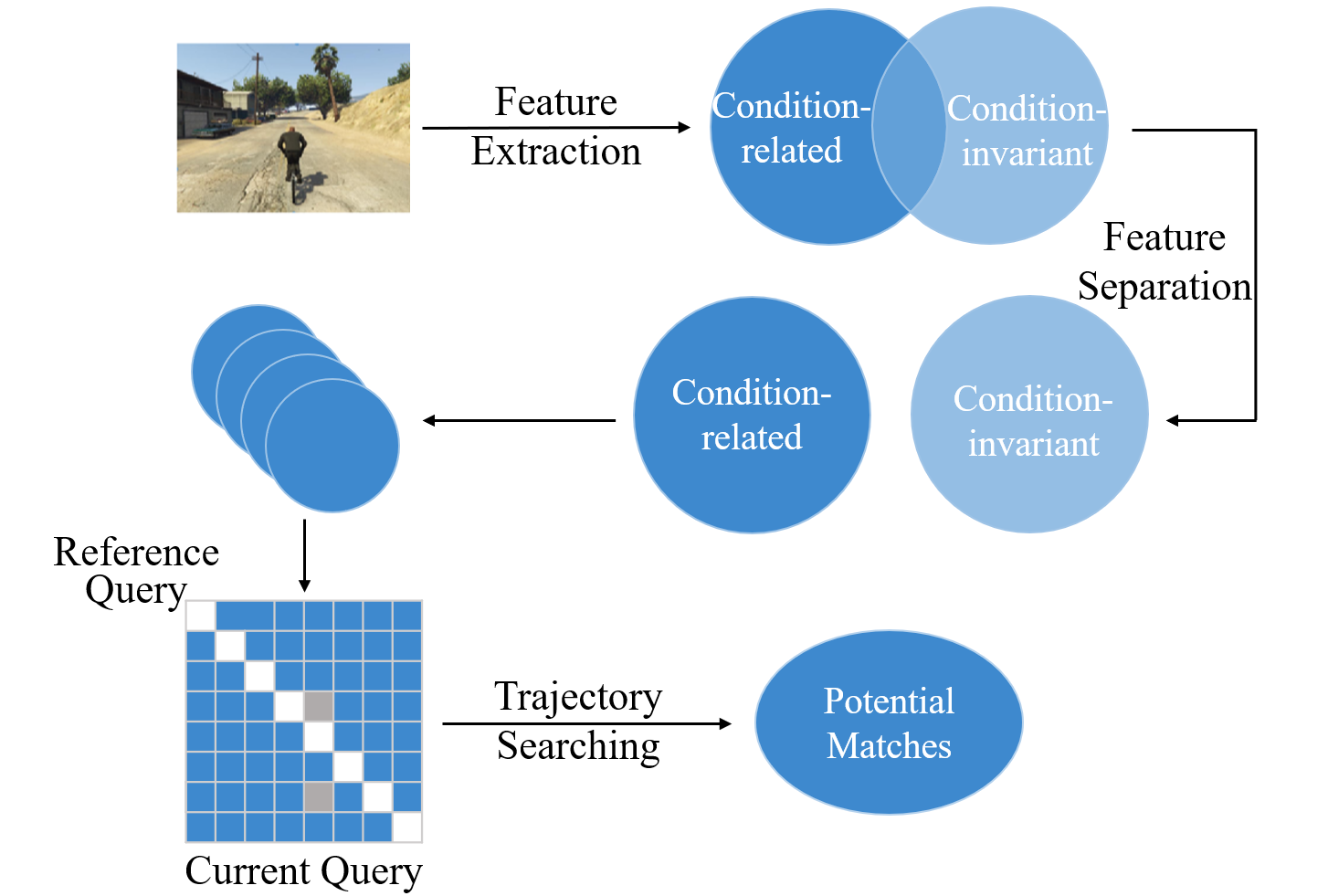
Figure 1: The pipeline of our proposed conditional visual place recognition method. In summary, there exists three core modules: 1) a CapsuleNet [12] based feature extraction module that is responsible for extracting condition-related and condition-invariant features from the raw visual inputs; 2) a condition enhanced feature separation module to further separate condition-related ones in the joint feature-distribution; 3) a trajectory searching mechanism for finding best matches based on the feature differences of query trajectory features.

Ideally, the place recognition method should be able to capture condition-invariant features for robust loop closure detection, since the appearance of scene objects (e.g., roads, terrains and houses) is often highly related to environmental conditions, and that each object has its own appearance distribution under variant conditions. To the best of our knowledge, there are few VPR methods that have explored how to improve the place recognition performance against variant environmental conditions [4]. A major drawback of these methods is that the change in environmental conditions affects the local features, resulting in decreased accuracy of VPR. In this paper, we propose the condition-directed visual place recognition method to address this issue. Our work consists of two parts: feature extraction and feature separation.

Firstly, in the feature extraction step, we utilize a CapsuleNet-based network [12] to extract multi-domain place features, as shown in Fig. 1. Traditional convolutional neural network (CNN) is efficient in object detection , regression and segmentation, but as pointed out by Hinton, the inner connections of objects are easily lost with the deep convolutional and max pooling operations. For instance, in face detection tasks, even if the facial objects (nose, eyes, mouth, lips) are in incorrect layouts, the traditional CNN method may still consider the image as a human face, since it contains all the necessary features of a human face. This problem also exists in place recognition tasks, since different places may contain similar objects but with different arrangements. CapsuleNet uses an dynamic routing method to cluster the shallow convolutional layer features in an unsupervised way. In this paper, we demonstrate another application of CapsuleNet, which could capture feature distribution under specific conditions.

The main contributions of this work can be summarized as follows:

• We propose the use of CapsuleNet-based feature extraction module, and show its robustness in the conditional feature learning for the visual place recognition task.

• We propose a feature separation method for the visual place recognition task, where features are indirectly separated based on the relationship between condition-related and condition-invariant features in an information-theoretic view.

The outline of the paper is as follows: Section II introduces the related works on visual-based place recognition methods. Section III describes our conditional visual place recognition method, which has two components: feature extraction and feature separation. In Section IV, we evaluate the proposed method on two challenging datasets: the NORDLAND [5] dataset which has same trajectories under multiple season conditions and a GTAV dataset which is generated on the same trajectory under different weather conditions in a game simulator. Finally, we provide concluding remarks in Section V.

II Related Work

Visual place recognition (VPR) methods have been well studied in past several years, and can be classified into two categories: feature- and appearance-based. In feature-based VPR, descriptive features are transformed into local place descriptors. Then, place recognition can be achieved by extracting the current place descriptors and searching similar place indexes in the bag of words. On the contrary, appearance-based VPR uses feature descriptors that are extracted from the entire image, and performs place recognition by assessing feature similarities. SeqSLAM [9] describes image similarities by directly using the sum of absolute difference (SAD) between frames, while vector of locally aggregated descriptors (VLAD) [15] aggregates local invariant features into a single feature vector and uses Euclidean distance between vectors to quantify image similarities.

Recently, many works have investigated CNN-based features for appearance-based VPR tasks. Sünderhauf et al. [14] first used pre-trained VGG model to extract middle-layer CNN outputs as image descriptors in the sequence matching pipeline. However, a pre-trained network can not be further trained for place recognition task, since the data labels are hard to define in VPR task. Recently, Chen et al. [2] and Garg et al. [4] address the conditional invariant VPR as an image classification task and rely on precise but expensive human labeling for semantic labels. Arandjelovic et al. [1] developed NetVLAD, which is a modified form of the VLAD features, with CNN networks to improve the feature robustness.

The approach that comes closest to our method is the work of Porav et al. [11], where they learn invertible generators based on the CycleGAN [8], The original CycleGAN method can transform the image from one domain to another domain, but such transformation is limited to only two domains. Thus, for multiple domain place recognition task, the method of Porav et al. requires transformation model between each pair of conditions. In contrast, our method can learn more than two conditions in the same structure.

III Proposed Method

In this section, we investigate the details of two core modules in our conditional visual place recognition method.

III-A Feature Extraction

III-A1 VLAD

VLAD is a feature encoding and pooling method, which encodes a set of local feature descriptors extracted from an image by using a clustering method such as K-means clustering. For the feature extraction module, we extract multi-domain place features from the raw image, by utilizing a CapsuleNet module. Let $q_{ik}$ be the strength of the association of data vector $x_{i}$ to the cluster $\mu_{k}$, such that $q_{ik}\geq 0$ and $\sum_{k=1}^{K}q_{ik}=1$, where $K$ is the clusters number. VLAD encodes feature $x$ by considering the residuals

$$v_{k}=\sum_{i=1}^{N}q_{ik}(x_{i}-\mu_{k}),$$ (1)

and the joint feature description $\{v_{1},v_{2},v_{3},...,v_{N}\}$, where $N$ is the local features number.

Assume we can extract $N$ lower feature descriptors (each is denoted as $x_{i}$) from the raw image, we can construct a new VLAD like module with the following equation,

$$v_{k}=\sum_{i=1}^{N}Q_{k}(l_{i})r(x_{i},\mu_{k}),$$ (2)

where $r(x_{i},\mu_{k})$ is the residual function measuring similarities between $x_{i}$ and $\mu_{k}$, and $Q_{k}(l_{i})$ is the weighting of capsule vector $l_{i}$ involved with the $k^{\text{th}}$ cluster center.

III-A2 Modified CapsuleNet

In order to transform Eq.2 into an end-to-end learning block, we consider two aspects:

1. Constructing the residual function $r(x_{i},\mu_{k})$;

2. Assigning the weights $Q_{k}(l_{i})$.

With lower layer features extracted from the shallow convolution layer, we use $N\times D_{property}$ matrix to map lower level features into higher level features, where $N$ is the CNN unit number in the shallow convolution layer.

If we want to integrate the lower-higher feature mapping within a single layer, the local lower level feature $x_{i}$ should have a linear mapping layer to represent the residual function $Q_{i}$

$$f(x_{i},\mu_{k}) =\mathbf{W}_{ik}x_{i}+b_{k}$$

$$r(x_{i},\mu_{k}) =f(x_{i},\mu_{k})-\frac{1}{N}\sum_{k}f(x_{i},\mu_{k}),$$ (3)

where $\mathbf{W}_{ik}$ and $b_{k}$ are the linear transformation weighting and bias for the $k^{\text{th}}$ capsule center.

Furthermore, to estimate the local capsule features weighting $Q_{k}(x_{i})$, we apply a soft assignment estimation defined as

$$Q_{k}(x_{i})=\frac{\exp(b_{ik})}{\sum_{j}^{K}\exp(b_{ij})},$$ (4)

where $b_{ik}$ is the probability that the $i^{\text{th}}$ local capsule feature belonging to $k^{\text{th}}$ capsule cluster $c_{k}$. Therefore, Eq.2 can be written in the following format,

$$v_{k}=\sum_{i=1}^{N}\frac{\exp(b_{ik})}{\sum_{j}^{K}\exp(b_{ij})}(f(x_{i},\mu_{k})-\frac{1}{N}\sum_{k}f(x_{i},\mu_{k})).$$ (5)

In order to learn the parameters $b_{ij},{W}_{ik}$, and $c_{k}$, we apply the iterative dynamic routing mechanism as described in [12]. For the output of $N_{object}$ higher level features, we assume the last $D_{C}$ dimensions are assigned as the condition features, e.g. $D_{C}=4$ is in the case where the condition is season.

III-B Feature Separation

In the previous section, we described the feature extraction module $p_{\theta}$. In this section, we use an additional decoder module $q_{\phi}$, and two reconstruction modules on feature $\mathcal{L}_{Feature}$ and image $\mathcal{L}_{Image}$ domain to achieve the feature separation. Naturally, condition-invariant feature $Z_{G}$ and condition-related feature $Z_{C}$ are highly correlated. Fig. 2 shows the relationship between information $Z_{G}$ and $Z_{C}$. $H(Z_{G},Z_{C})$ and $I(Z_{G};Z_{C})$ are the joint entropy and the mutual entropy respectively, while $H(z_{G}|z_{C})$ and $H(z_{C}|z_{G})$ are the conditional entropy. From the view of information theory, feature separation can be achieved in the following ways:

• Decrease the conditional entropy $H(z|x)$: less conditional entropy enforces the unique mapping from $x\in\chi$ to $z\in(Z_{G},Z_{C})$;

• Improve the geometric feature extraction capability: the more accurate geometry we capture, the higher LCD accuracy we can achieve;

• Reduce the mutual entropy $I(Z_{G};Z_{C}|x)$: use environmental conditions to direct feature extraction.

We add these three restrictions in our feature separation module.

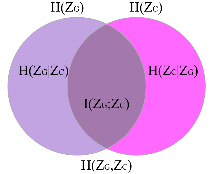
Figure 2: The relationship of condition-related $Z_{C}$ and condition-invariant $Z_{G}$ feature in the information theory view.

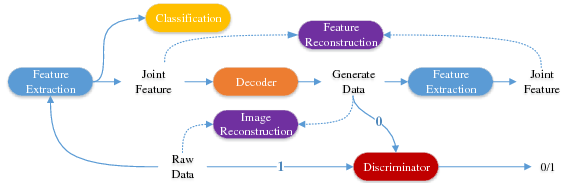
Figure 3: The framework of feature separation. The networks are combined with four modules: the feature extraction module as given in the previous section; a classification module estimating the environmental conditions; a decoder module mapping the extracted feature back to the data domain; a discriminator module distinguishing the generated data and raw data; and two reconstruction loss modules on data and feature domain respectively.

III-B1 Conditional Entropy Reduction

$H(z|x)$ measures the uncertainty of feature $z$ given the data sample $x$. The conditional entropy $H(z|x)=0$ can be achieved, if and only if $z$ is the deterministic mapping of $x$. Thus, reducing $H_{p_{\theta}}(z|x)$ can improve the uniqueness mapping from $x$ to $z$, where $p_{\theta}$ is the parameter in the encoder module. However, improving the condition entropy $H_{p_{\theta}}(z|x)$ is intractable, since we can not access the data-label pair $(x,z)$ directly. An alternative approach is to optimize the upper bound of $H_{p_{\theta}}(z|x)$, and the upper bound can be obtained through the following equation,

$$\min_{\theta,\phi}H_{p_{\theta}}(z|x) \triangleq\min_{\theta,\phi}-\sum p_{\theta}(z|x)\log(p_{\theta}(z|x))$$

$$=\min_{\theta,\phi}-\sum p_{\theta}(z|x)[\log(q_{\phi}(z|x))]$$

$$-\sum p_{\theta}(z|x)[\log(p_{\theta}(z|x))-\log(q_{\phi}(z|x))]$$

$$=\min_{\theta,\phi}H_{p_{\theta}(z|x)}[\log(q_{\phi}(z|x))]$$

$$-E_{p_{\theta}(z|x)}[\mathbf{KL}(p_{\theta}(z|x)\|(q_{\phi}(z|x)))],$$ (6)

where $\mathbf{KL}$ is the Kullback-Leibler divergence. And $H_{p_{\theta}}(\log(q_{\phi}(z|x)))$ measures the uncertainty of the predicted feature with a given sample data $x$. Since we can not extract features from the $q_{\theta}$ directly, we add an additional feature encoder module after the decoder module (see Fig .3). Eq. 6 can be converted into

$$\min_{\theta,\phi}H(z|x) \leq\min_{\theta,\phi}H_{p_{\theta}(z|x)}[\log(q_{\phi}(z|x))]$$

$$\triangleq\min_{\theta,\phi}H_{\hat{z}\sim p_{\theta}(z|x),\hat{x}\sim q_{\phi}(x|\hat{z})}[\log(p_{\theta}(z=\hat{z}|\hat{x}))]$$

$$=\mathcal{L}_{Feature}(z,\hat{z}),$$ (7)

where $\mathcal{L}_{Feature}$ is the Feature Reconstruction Loss between feature extracted from the raw data and the reconstructed data. As we can see in Eq. 7, the original $H_{p_{\theta}}(z|x)$ is transformed into its upper bound $\mathcal{L}_{Feature}(z,\hat{z})$, and the upper bound is reduced only when the feature domain and data domain are perfectly matched.

III-B2 Feature Extraction Improvement

Condition entropy reduction sub-module can restrict the mapping uncertainty from data domain to the feature domain, this restriction is highly related to the generalization ability of the encoder module. For the place recognition task, there will be highly diverse scenes in practice, however, we can only generate limited samples for network training. In theory, the GAN method use a decoder and discriminator module can learn the the potential feature-to-data transformation with limited samples. Thus, we improve the data generalization ability by applying GANs.

$$\mathcal{L}_{GAN}=\min_{\phi}\max_{\omega}E(\log(D_{\omega}(x))+$$ (8)

$$E_{x\sim q_{\phi}(x|z)}(\log(1-D_{\omega}(x))).$$

As demonstrated by Goodfellow et.al [6], with iterative updating of the decoder module $q_{\phi}$ and the discriminator module $D_{\omega}$, GAN could pull the generated data distribution closer to the real data distribution, and improve the generalization ability of the decoder module $q_{\phi}$.

III-B3 Mutual entropy reduction

$I(z_{G};z_{C}|x)$ is the mutual entropy, which can be extended by

$$I(z_{G};z_{C}|x)= H(z_{G}|x)+H(z_{C}|x)-H(z_{G},z_{C}|x),$$ (9)

where, reducing the mutual entropy is equivalent to reducing the right-hand term in the above equation. Since the conditional entropy satisfies $0\leq H(z_{G},z_{C}|x)$ , we can find the upper bound of $I(z_{G};z_{C}|x)$ by ignoring $H(z_{G},z_{C}|x)$

$$\min_{\theta}I(z_{G};z_{C}|x) \leq\min_{\theta}(H(z_{G}|x)+H(z_{C}|x)).$$ (10)

For the condition-related features, we apply a soft-max based classification module $\mathcal{L}_{Cond}$, to reduce the conditional entropy $H(z_{C}|x)$. Furthermore, we apply an $L_{2}$ image reconstruction loss to further restrict the uncertainty $H(z_{G}|x)$ given a sample data $x$,

$$\mathcal{L}_{Image}=\|x_{raw}-x_{reco}\|,$$ (11)

where $x_{raw}$ and $x_{reco}$ are the raw image and reconstructed one respectively.

By combining Eq.[7, 8, 11] and $\mathcal{L}_{Cond}$, the joint loss function can be obtained as

$$\mathcal{L}_{Joint}= \mathcal{L}_{Feature}+\mathcal{L}_{GAN}+\mathcal{L}_{Cond}+\mathcal{L}_{Image}.$$ (12)

IV Experiment Results

In this section, we analyze the performance of our method on two datasets and compare it with three feature extraction methods for the visual place recognition task. The experiments are conducted on a single NVIDIA 1080Ti card with 64G RAM on the Ubuntu 14.04 system. For our method, our can inference the local place image with just $30ms$, and each feature is just $1kb$.

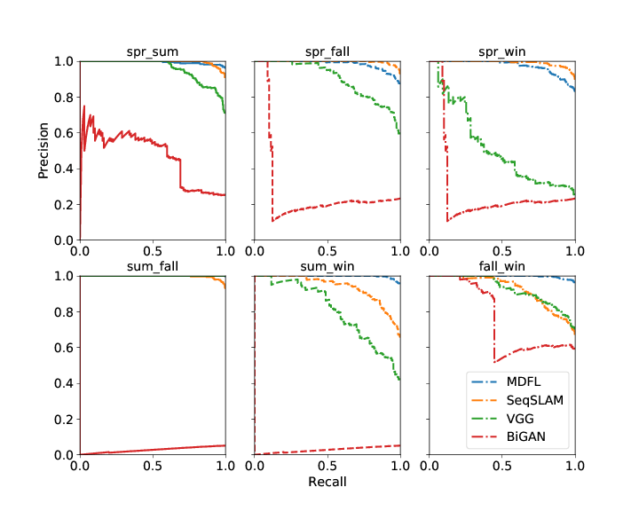
(a) Nordland datasets

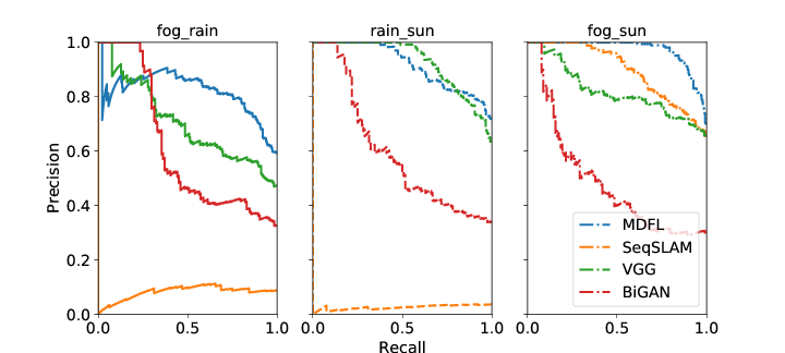
(b) GTAV datasets

Figure 4: Precision-Recall curve of various VPR methods on the two datasets. The method is considered to be good if the curve is in the upper-right corner. As we see, MDFL outperforms other methods in most of the cases.

IV-A Datasets

The datasets we used here are the Nordland dataset [13] and the GTAV dataset [16]. The Nordland dataset was recorded on a train in Norway during four different seasons, and each sequence follows the same track. In each sequence, we generate $17885$ frames from the video at $12$ Hz, and the first $16885$ frames of each sequence is used for training, and the last $1000$ frames for testing. Note that we train on all four Norldand seasonal datasets, using the seasonal labels to find the condition dependent/invariant features, and then test on the last 1000 frames of each dataset. In the training procedure, we randomly select frames and their corresponding status labels from the four sequences.

The second dataset GTAV [16] contains trajectories on the same track under three different weather status (sunny, rainy and foggy). This dataset is more challenging than the Nordland dataset, since the viewpoints are variant in the GTAV dataset. We generate more than $10,000$ frames in each sequence, $9000$ frames are used as training data, and the remaining $1000$ frames for testing.

For each dataset, all images are resized to $64\times 64\times 3$ in RGB format. The loop closure detection mechanism is followed as in the original SeqSLAM method; sequences of image features are matched instead of a single image. For more details about the structure of the SeqSLAM, we refer the reader to [9].

IV-B Accuracy Analysis

To investigate the place recognition accuracy, we compare our feature extraction method with three methods in sequential matching: the original feature in SeqSLAM that uses sum of absolute difference as local place feature description; convolution layer feature from VGG network, which is trained on the large-scale image classification dataset [10]; adversarial feature learning-based unsupervised feature obtained from the generative adversarial networks [3]; The place is considered as being matched when the distance between current frame and target frame is limited within 10 frames. We evaluate the performances in the precision-recall curve (PR-curve), area under curve (AUC) index, inference time, and storage requirement.

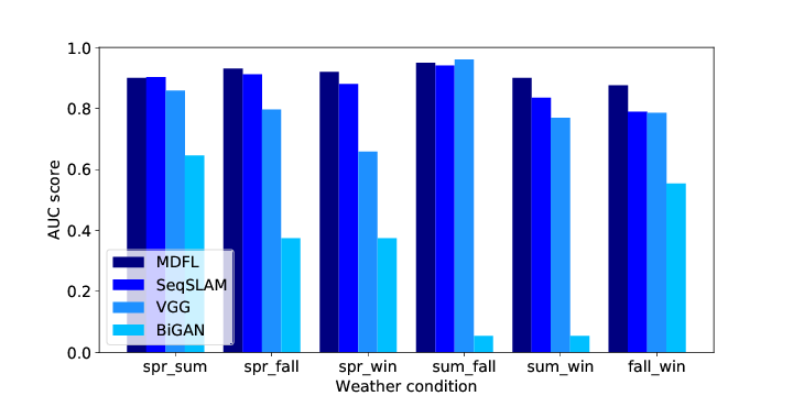
(a) AUC on Nordland datasets

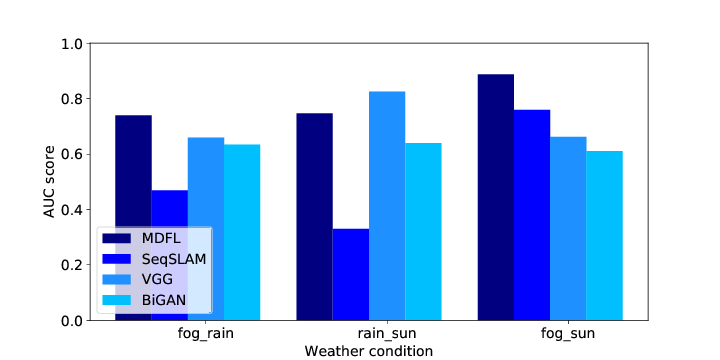
(b) AUC on GTAV datasets

Figure 5: AUC index of the various VPR methods. The methods match images from the two datasets under different conditions.

Fig.4 and  5 show the precision-recall curve and AUC index respectively for all the methods on the Nordland datasets and the GTAV datasets. In Fig. 5, the label spr-sum, spr-fall, etc. refer to the performance using the same network and same model, with different testing sequences.

In general, all the methods perform better in the Nordland dataset than in the GTAV dataset, since the viewpoints are stable and the geometric changes are smooth due to the constant speed of the train. In contrast, test sequences in GTAV datasets have significant viewpoints differences. Furthermore, limited field of view and multiple dynamic objects in GTAV also introduces additional feature noises, which causes a significant difference in scene appearance.

VGG features perform well under normal conditions, such as summer-winter in Nordland, but perform poorly under unusual conditions, which indicates that the VGG features trained on normal environmental conditions do not generalize. BiGAN does not perform well on either datasets, and this is mainly because it does not take into account the condition of the scene and considers all the images as a joint manifold. For example, the same place under different weather conditions will be encoded differently using BiGAN. Since SeqSLAM uses gray images to ignore the appearance changes under different environmental conditions, the image based features in SeqSLAM are robust against changing conditions as we can see in the Nordland dataset. However, its matching accuracy decreases greatly in the GTAV dataset, since raw image features are very sensitive to the changing viewpoints.

In general, MDFL outperforms the above features in most cases of the NORDLAND and GTAV datasets, and can handle complex situation well, but is not the best in some situations, such as spring-summer in NORDLAND and rain-summer in GTAV. One potential reason is that, in each dataset, we only consider one type of environmental condition (Season or weather), but we did not take into account the illumination changes. Since the illumination changes continuously, it is not easy to set this type of environmental condition in training. The geometric features instructed by the environment labels can capture more common geometry details among the multiple weather or season conditions. Another advantage lies in the structure of the CapsuleNet-like architecture that enables MDFL to cluster lower level geometry features into high level descriptions. The benefit of this mechanism can be better seen in the GTAV dataset, where the extracted features are more robust to the viewpoints difference. Table I shows the average AUC results of different methods in both datasets, and our MDFL method outperforms all the other methods.

TABLE I: Average AUC index on Nordland and GTAV datasets

Dataset	Caps	SeqSLAM	VGG16	BiGAN
GTAV	0.790	0.518	0.715	0.627
Nordland	0.912	0.876	0.804	0.345

V Conclusion

In this paper, we propose a novel multi-domain feature learning method for visual place recognition task. At the core of our framework lies the idea of extracting condition-invariant features for place recognition under various environmental conditions. We use a CapsuleNet-based module to capture multi-domain features from the raw image, and apply a feature separation module to indirectly separate condition-related and condition-invariant features. Based on the extracted condition-invariant features, experiments on the multi-season condition NORDLAND dataset and the multi-weather condition GTAV datasets, demonstrate the robustness of our method. The major limitation for our method is that the shallow layer CapsuleNet-based module can only cluster lower level features, and can not capture the semantic descriptions for the place recognition. In our future work, we will investigate hierarchical CapsuleNet network module to extract higher level semantic features for place recognition.

References

- Arandjelovic et al. [2016] Relja Arandjelovic, Petr Gronat, Akihiko Torii, Tomas Pajdla, and Josef Sivic. Netvlad: Cnn architecture for weakly supervised place recognition. In Proceedings of the IEEE Conference on Computer Vision and Pattern Recognition, pages 5297–5307, 2016.
- Chen et al. [2017] Z. Chen, A. Jacobson, N. Sünderhauf, B. Upcroft, L. Liu, C. Shen, I. Reid, and M. Milford. Deep learning features at scale for visual place recognition. In 2017 IEEE International Conference on Robotics and Automation (ICRA), pages 3223–3230, May 2017. doi: 10.1109/ICRA.2017.7989366.
- Donahue et al. [2016] Jeff Donahue, Philipp Krähenbühl, and Trevor Darrell. Adversarial feature learning. arXiv preprint arXiv:1605.09782, 2016.
- Garg et al. [2017] S. Garg, A. Jacobson, S. Kumar, and M. Milford. Improving condition- and environment-invariant place recognition with semantic place categorization. In 2017 IEEE/RSJ International Conference on Intelligent Robots and Systems (IROS), pages 6863–6870, Sept 2017. doi: 10.1109/IROS.2017.8206608.
- Geiger et al. [2013] Andreas Geiger, Philip Lenz, Christoph Stiller, and Raquel Urtasun. Vision meets robotics: The kitti dataset. The International Journal of Robotics Research, 32(11):1231–1237, 2013.
- Goodfellow et al. [2014] Ian Goodfellow, Jean Pouget-Abadie, Mehdi Mirza, Bing Xu, David Warde-Farley, Sherjil Ozair, Aaron Courville, and Yoshua Bengio. Generative adversarial nets. In Advances in neural information processing systems, pages 2672–2680, 2014.
- Lowry et al. [2016] S. Lowry, N. Sünderhauf, P. Newman, J. J. Leonard, D. Cox, P. Corke, and M. J. Milford. Visual place recognition: A survey. IEEE Transactions on Robotics, 32(1):1–19, Feb 2016. ISSN 1552-3098. doi: 10.1109/TRO.2015.2496823.
- Lu et al. [2017] Yongyi Lu, Yu-Wing Tai, and Chi-Keung Tang. Conditional cyclegan for attribute guided face image generation. arXiv preprint arXiv:1705.09966, 2017.
- Milford and Wyeth [2012] M. J. Milford and G. F. Wyeth. Seqslam: Visual route-based navigation for sunny summer days and stormy winter nights. In 2012 IEEE International Conference on Robotics and Automation, pages 1643–1649, May 2012. doi: 10.1109/ICRA.2012.6224623.
- Muhammed et al. [2017] M. A. E. Muhammed, A. A. Ahmed, and T. A. Khalid. Benchmark analysis of popular imagenet classification deep cnn architectures. In 2017 International Conference On Smart Technologies For Smart Nation (SmartTechCon), pages 902–907, Aug 2017. doi: 10.1109/SmartTechCon.2017.8358502.
- Porav et al. [2018] Horia Porav, Will Maddern, and Paul Newman. Adversarial training for adverse conditions: Robust metric localisation using appearance transfer. arXiv preprint arXiv:1803.03341, 2018.
- Sabour et al. [2017] Sara Sabour, Nicholas Frosst, and Geoffrey E Hinton. Dynamic routing between capsules. In Advances in Neural Information Processing Systems, pages 3859–3869, 2017.
- Sünderhauf et al. [2013] Niko Sünderhauf, Peer Neubert, and Peter Protzel. Are we there yet? challenging seqslam on a 3000 km journey across all four seasons. In Proc. of Workshop on Long-Term Autonomy, IEEE International Conference on Robotics and Automation (ICRA), page 2013. Citeseer, 2013.
- Sünderhauf et al. [2015] N. Sünderhauf, S. Shirazi, F. Dayoub, B. Upcroft, and M. Milford. On the performance of convnet features for place recognition. In 2015 IEEE/RSJ International Conference on Intelligent Robots and Systems (IROS), pages 4297–4304, Sept 2015. doi: 10.1109/IROS.2015.7353986.
- Wang et al. [2016] Y. Wang, Y. Cen, R. Zhao, S. Kan, and S. Hu. Fusion of multiple vlad vectors based on different features for image retrieval. In 2016 IEEE 13th International Conference on Signal Processing (ICSP), pages 742–746, Nov 2016. doi: 10.1109/ICSP.2016.7877931.
- Yin et al. [2017] Peng Yin, Yuqing He, Na Liu, and Jianda Han. Condition directed multi-domain adversarial learning for loop closure detection. arXiv preprint arXiv:1711.07657, 2017.
- Zhou et al. [2016] H. Zhou, K. Ni, Q. Zhou, and T. Zhang. An sfm algorithm with good convergence that addresses outliers for realizing mono-slam. IEEE Transactions on Industrial Informatics, 12(2):515–523, April 2016. ISSN 1551-3203. doi: 10.1109/TII.2016.2518481.