Controllable dispersion of domain wall movement in antiferromagnetic thin films at finite temperatures

Abstract

The dynamics of a 90^∘ domain wall in an antiferromagnetic nanostrip driven by the current-induced spin-orbital torque are theoretically examined in the presence of random thermal fluctuations. A soliton-type equation of motion is developed on the basis of energy balance between the driving forces and dissipative processes in terms of the domain wall velocity. Comparison with micromagnetic simulations in the deterministic conditions shows good agreement in both the transient and steady-state transport. When the effects of random thermal fluctuations are included via a stochastic treatment, the results clearly indicate that the dispersion in the domain wall position can be controlled electrically by tailoring the strength and duration of the driving current mediating the spin orbital torque in the antiferromagnet. More specifically, the standard deviation of the probability distribution function for the domain wall movement can be tuned widely while maintaining the average position unaffected. Potential applications of this unusual functionality include the probabilistic computing such as Bayesian learning.

I Introduction

Effective control of the domain walls (DWs) in the antiferromagnetic (AFM) materials remains a vital challenge for the prospective spintronic applications Gomonay2017 ; Baltz2018 . A number of approaches explored thus far have demonstrated the promise. For instance, the effect of the spin-transfer torque was able to manipulate the AFM DWs Hals2011 ; Swaving2011 ; Tveten2013 . Similarly, the AFM DW transfer can be induced as a result of the spin-wave mediated forces Kim2014 ; Tveten2014 , which are enhanced by the Dzyaloshinskii-Moriya interaction Qaiumzadeh2018 . In fact, the Dzyaloshinskii-Moriya interaction also assists the DW movement in the presence of a rotating magnetic field Pan2018 . Further, the normally ineffective magnetic field was shown to control the AFM DW velocity when its spatial gradient is combined with a charge current or more precisely, the spin transfer effect Rodrigues2017 ; Yamane2017 . However, the most accessible mechanism for the control of DW dynamics in the AFM thin films appears to be the spin-orbital torque (SOT). The electric current through a non-centrosymmetric antiferromagnet generates a SOT associated with a staggered (or Néel-order) field Gomonay2016 ; Yu2018 . The DW motion can also be modulated by the SOT induced at the interface with a strongly spin-orbit coupled material such as a heavy metal Shiino2016 .

Specific physical details aside, all of the aforementioned studies have considered the deterministic dynamics essentially in the limit of zero temperature. Furthermore, most of them have focused on the AFM textures in the form of 180^∘ DWs, posing an additional challenge in discriminating the domains with antiparallel Néel vectors. A more promising alternative may be to utilize the 90^∘ DWs in light of the recent experimental advances in their manipulation and detection Yu2018 . In fact, 90^∘ rotation of the Néel-vector orientation has already been identified in the electrical measurements with a large signal in the anisotropic magnetoresistance Yu2018 or its tunneling variety Park2011 . On the other hand, the theoretical understanding on the dynamics of 90^∘ DWs in the antiferromagnets has received only limited attention Gomonay2016 . Since the operation is predominantly at the ambient conditions, the effect of finite temperature and subsequent stochastic nature of the DW dynamics also add interesting perspectives.

The uncertainty in the final DW position is evidently undesirable for memory or Boolean logic applications. On the other hand, controllable stochasticity of the output signals with a desired distribution function has begun to draw much attention since its prospective utilization in machine learning or Bayesian computing. Physical implementation of the concept of probabilistic computing has so far relied predominantly on the external generators of random numbers. While the alternative approaches have also been explored, they tend to involve complex hardware arrangements (see, for instance, Ref. Pinna2018 and the references therein). It is clearly desirable if a single device or structure can meet the needs with simple electrical control. The probabilistic effect of the AFM DW motion may offer this unique functionality.

In the present work, we theoretically analyze the 90^∘ DW motion in an AFM thin film driven by the SOT pulse at finite temperatures. A soliton-type treatment is developed from the Lagrangian representation to examine the DW dynamics including the effect of random thermal fluctuations. The results clearly illustrate the characteristics of the AFM DW motion. When subjected to a SOT pulse, the DW undergoes acceleration and then velocity saturation as the dissipation compensates the anti-damping torque. Once the driving force is turn off, the inertial phase follows much like an actual particle with non-zero mass. The random thermal fields introduce substantial deviations in the DW trajectories depending on the strength and the duration of the driving SOT pulse. The corresponding variation in the probability distribution of the DW position indicates a broad range that can be tuned electrically.

II Theoretical formulation

The structure under consideration is shown in Fig. 1(a). It is essentially a bilayer structure of an AFM nanostrip and a strongly spin-orbit coupled material that can benefit from the current induced SOT mentioned earlier Shiino2016 . A vertical tunnel junction can be added on top for electrical measurement of the DW position via the tunneling anisotropic magnetoresistance. As the $x$-directional current flow induces the effective field along the $z$ axis in the present set-up, the magnetic domains need to be oriented normal to this axis ($z$) for efficiency. Accordingly, an antiferromagnet with biaxial anisotropy in the $x$-$y$ easy plane (such as those with tetragonal $D_{4h}$ symmetry) is assumed for the desired 90^∘ DW. The metallic materials are expected to offer a convenient choice for experimental realization and detection, while the similar physical principles can be applied to the dielectric systems as well.

In the analysis, the relatively small cross-section of the AFM strip makes it possible to ignore the Néel-vector variation in the $y$-$z$ plane, reducing the problem to the dynamics in the 1+1 space-time ($x$,$t$) coordinates with no additional variables. Since the Néel-vector reorientation is only in the $x$-$y$ plane, the calculation can take advantage of the Lagrangian representation in terms of the azimuthal angle $\varphi(x,t)$ between the two easy axes (using the $x$ as the reference). A similar formalism developed earlier for an easy-plane antiferromagnet Semenov2017 can be directly generalized to the case of biaxial anisotropy with the following term for the anisotropy energy,

$$W_{in}=\frac{K}{4}(n_{x}^{4}+n_{y}^{4})=\frac{K}{8}\sin^{2}2\varphi.$$ (1)

Here, $K$ ($<0$) is the anisotropy constant and $n_{x(y)}=L_{x(y)}/\left|\mathbf{L}\right|=\cos\varphi$ ($\sin\varphi$) is the normalized representation $\mathbf{n}$ of the Néel vector $\mathbf{L}$. The $z$-component ($n_{z}$) does not appear in the dynamical equations due to the hard nature of this direction Semenov2017 . Then, the dimensionless Lagrangian $\textswab{L}=\textswab{L}/\left|K\right|$ can be reduced to the canonical form in terms of dimensionless time $t$ ($=\omega_{r}t$) and space $x$ ($=\omega_{r}x/v_{m}$); i.e.,

$$\textswab{L}=\frac{1}{2}\dot{\varphi}_{(t)}^{2}-\frac{1}{2}\dot{\varphi}_{(x)}^{2}-\frac{1}{8}\sin^{2}2\varphi,$$ (2)

where $\dot{\varphi}_{(i)}\equiv\frac{\partial}{\partial i}\varphi$ ($i=x,t$), $\omega_{r}=\gamma\sqrt{2H_{\mathrm{ex}}H_{\mathrm{an}}}$ denotes the zero-field AFM resonance frequency, $\gamma$ the gyromagnetic ratio, $H_{\mathrm{an}}=\left|K\right|/\frac{1}{2}L$ the anisotropy field, $H_{\mathrm{ex}}$ the exchange field between the magnetic sublattices, and $v_{m}$ the magnon velocity.

The corresponding Euler-Lagrange equation for an open system subjected to the external forces (i.e., torques) $\rho=\rho(x,t)$ reads

$$\ddot{{\varphi}}_{(tt)}-\ddot{{\varphi}}_{(xx)}+\frac{1}{4}\sin 4\varphi=\rho.$$ (3)

It is remarkable that Eq. (3) reproduces the sine-Gordon equation in terms of variable $4\varphi$ for a conserving system (i.e., when $\rho=0$). In this case, the basic solution of Eq. (3) can be expressed in the form of a soliton moving with velocity $v$,

$$\varphi=\pm\arctan\left[\exp\left(\frac{x-vt}{\sqrt{1-v^{2}}}\right)\right].$$ (4)

The effective width $\delta_{\mathrm{dw}}$ of the soliton (or the DW) can be estimated as $\pi\sqrt{1-v^{2}}$. The corresponding Néel-vector texture $\mathbf{n}=(\cos\varphi,\sin\varphi,0)$ is shown in Fig. 1(b). Note that the velocity $v$ is also normalized to $v_{m}$ following the definitions of $x$ and $t$ (thus, $\left|v\right|<1$).

Similarly to Ref. Shiino2016 , the soliton representation [Eq. (4)] of the DW texture is treated as an ansatz for the analysis of a non-conserving system with energy dissipation and external forces. In such an approximation, only the DW velocity $v=v(x,t)$ remains the actual parameter describing the DW dynamics. To proceed further, the specific form for $\rho$ is needed in Eq. (3). The relevant contributions in the present analysis come from three terms$-$the energy dissipation via damping, the anti-damping SOT from the driving current, and the field-like torque from the random thermal fluctuations. The resulting expression for $\rho(x,t)$ is given in dimensionless units as Semenov2017

$$\rho=-2\lambda\dot{\varphi}_{(t)}+\Phi(x,t)-\frac{\partial h_{\mathrm{th}}}{\partial t}\,,$$ (5)

where $\lambda$ ($=\delta_{r}/\omega_{r}$) is the damping parameter related to the width $\delta_{r}$ of the AFM resonance and $h_{\mathrm{th}}$ ($=\gamma H_{\mathrm{th}}/\omega_{r}$) is the normalized thermal field $H_{\mathrm{th}}$. In addition, the second term representing the anti-damping SOT of $\eta(\mathbf{n\times}\hat{\mathbf{z}})\cdot\dot{\mathbf{n}}_{(t)}$ takes the form

$$\Phi(x,t)=\frac{\eta(x,t)}{M_{L}^{2}}\frac{H_{\mathrm{ex}}}{2H_{\mathrm{an}}},$$ (6)

where $M_{L}$ denotes the sublattice magnetization ($\simeq\frac{1}{2}L$) and the parameter $\eta$ reflects the strength of the spin-Hall current flowing into the AFM layer Shiino2016 . $H_{\mathrm{th}}$ is a natural source of randomness in the DW trajectories and the dispersion in its final location. With corresponding modifications to Eq. (5), the formalism discussed above can also be applied to the DW transfer driven by the Néel SOT in the asymmetric antiferromagnets Gomonay2016 .

The dynamics of the Néel-vector textures are first examined in the absence of thermal fluctuations, where the current induced SOT unambiguously determines the DW motion. Applying the ansatz of Eq. (4) sufficiently simplifies the problem to the balance of energy flows to and from the DW, avoiding the need to solve Eqs. (3) and (5) directly. In this context, the net mechanical energy of the DW with the Lagrangian given in Eq. (2) becomes

$$E(v)=\int\left(\frac{1}{2}\dot{\varphi}_{(t)}^{2}+\frac{1}{2}\dot{\varphi}_{(x)}^{2}+\frac{1}{8}\sin^{2}2\varphi\right)dx.$$ (7)

The range of integration can be safely set for the entire $x$-axis provided that the structure is much longer than the DW width. Then, for a single 90^∘ wall of Eq. (4), the calculation yields

$$E(v)=\frac{1}{2\sqrt{1-v^{2}}},$$ (8)

which corresponds to the $1/16$ of the energy for the 360^∘ kink described by the sine-Gordon equation. The description in conventional energy units can be restored by multiplying Eq. (8) by the factor $AKv_{m}/\omega_{r}$ and replacing $v$ with $v/v_{m}$. Here, $A$ denotes the cross section of the AFM thin film. Along with Eq. (8), the rate of net energy change (${dE}/{dt}$) can also be obtained from Eq. (5) as $\int[\Phi-2\lambda\dot{\varphi}_{(t)}]\dot{\varphi}_{(t)}dx$. After some algebra, the balance of energy flow to and from the AFM layer can be written finally in terms of an equation for the DW velocity

$$\frac{1}{2\lambda}\frac{dv}{dt}=\left(-v+Q\sqrt{1-v^{2}}\right)(1-v^{2}),$$ (9)

where $Q=\frac{\pi}{2\lambda}\Phi$. The solution of this expression provides the trajectory of the DW in the deterministic transport (i.e., no thermal fluctuations).

The equation of motion for the DW can be solved analytically under simple conditions. Assuming the initial stationary state $x=0$ at $t=0$ and a constant SOT $Q$ applied for a duration $t_{p}$, Eq. (9) yields

$$v_{Q}(t)=\frac{Q(1-e^{-2\lambda t})}{\sqrt{Q^{2}(1-e^{-2\lambda t})^{2}+1}},~{}~{}0<t\leq t_{p}.$$ (10)

The DW velocity increases linearly as $v_{Q}(t)=2\lambda Qt=\pi\Phi t$ in the beginning stage and then shows a saturation pattern once the dissipation compensates the anti-damping SOT as $t\gg 1/2\lambda$,

$$v_{s}=\frac{Q}{\sqrt{Q^{2}+1}}.$$ (11)

Note that this steady-state velocity $v_{s}$ reaches the maximal magnon velocity $v_{m}$ (=1) in the limit of $\lambda\rightarrow 0$ or $Q\rightarrow\infty$. Another interesting observation from Eq. (9) is that the velocity does not drop to zero even after the driving force is turned off. With the initial velocity of $v_{p}$ at $t=t_{p}$ [i.e., $v_{p}=v_{Q}(t_{p})$], the solution illustrates the characteristic inertial motion with

$$v_{0}(t)=\frac{v_{p}}{\sqrt{e^{4\lambda(t-t_{p})}(1-v_{p}^{2})+v_{p}^{2}}},~{}~{}t>t_{p}.$$ (12)

The dynamics overall appear much like those of actual particles with non-zero mass. In contrast, the DWs in a ferromagnet would stop moving as soon as the external torque ceases.

The AFM DW trajectory in the real space can be subsequently calculated by integrating the velocity over time. When the time of interest is longer than the pulse duration, the distance of travel includes the contribution by the inertia given by

$$x_{p}(t)=\frac{1}{4\lambda}\ln\left(\frac{1+v_{p}}{1-v_{p}}\times\frac{1-v_{0}(t)}{1+v_{0}(t)}\right),~{}~{}t>t_{p}.$$ (13)

Interestingly, this expression also characterizes the length that a DW moving with the velocity $v_{p}$ would travel unpropelled before losing all of the energy and coming to a stop (i.e., via inertia):

$$x_{p}(t\rightarrow\infty)~{}~{}{\Rightarrow}~{}~{}x_{\mathrm{in}}(v_{p})=\frac{1}{4\lambda}\ln\frac{1+v_{p}}{1-v_{p}}.$$ (14)

Another factor that must be considered in the DW movement is the effect of the coercivity. In the real structures, the defects like the grain boundaries and impurities may pin the DW. They keep the DW from slipping via the Brownian thermal motion. Otherwise, the diffusive dispersion in the DW position would diverge as time $t$ goes to infinity Yan2018 . The present formalism can readily account for the non-zero coercivity by introducing a lower bound to the kinetic energy for displacement. In this picture, the DW gets pinned as soon as the kinetic energy [$E(v)-E(0)$; see Eq. (8)] becomes smaller than the trapping energy $H_{c}M_{L}A\delta_{\mathrm{dw}}$, where $H_{c}$ denotes the effective field for coercivity. The impact of finite coercivity is particularly relevant during the inertial phase of the DW transport where the unpropelled movement is susceptible to the external factors. While the DW is being driven ($t\leq t_{p}$) on the other hand, we may not need an additional consideration so long as the applied SOT is sufficiently strong. A corresponding criterion can be expressed in terms of the critical velocity $v_{c}=\sqrt{4\pi H_{c}M_{L}/\left|K\right|}$ provided $v_{c}\ll 1$. Since $H_{c}$ cannot be determined a priori in terms of the material parameters, $v_{c}$ is treated as an independent phenomenological constant for the coercivity of a particular structure.

The expressions given above provide a complete solution to the problem of the DW dynamics driven by an electric current pulse. Under the pulse duration $t_{p}$ with amplitude $Q$, the net displacement becomes

$$x_{0}=x_{Q}(t_{p})+x_{\mathrm{in}}(v_{p})-x_{\mathrm{in}}(v_{c}),$$ (15)

where $x_{Q}(t_{p})$ [$=\int_{0}^{t_{p}}v_{Q}(t)dt$] denotes the distance traveled while being driven and $x_{\mathrm{in}}(v_{c})$ accounts for the reduction in the free flight (i.e., the inertial transport) due to the coercivity. Conversely, they can also be solved to deduce the relationship between $t_{p}$ and $Q$ for the desired $x_{0}$. It is evident that a shorter pulse duration is sufficient when the SOT amplitude is stronger and vice versa.

III Results and Discussion

III.1 Model validation

Before proceeding further, it is necessary to examined the validity of the adopted treatment based on the soliton description [Eq. (4)]. For this, a direct comparison is made with the micromagnetic simulation of the AFM DW dynamics Li2017 . The calculations are carried out for the AFM slab with the dimensions of 200$\times$50$\times$20 nm³. The numerical values assumed for the parameters are the sublattice magnetization $M_{L}=4\pi\times 320$ G, the anisotropy energy $K=-1.6\times 10^{6}$ erg$\cdot$cm^-3, the resonant frequency $\omega_{r}=2\pi\times 122$ GHz, and the damping parameter $\lambda=0.086$. In addition, the exchange stiffness $A_{\mathrm{ex}}$ of $10^{-7}$ erg/cm is used that further specifies the magnon velocity $v_{m}$ of $6.9\times 10^{5}$ cm/s ($=\gamma\sqrt{A_{\mathrm{ex}}H_{\mathrm{ex}}/M_{L}}$) Gomonay2016 . The relation between the SOT $Q$ and the current density $J$ (i.e., $Q/J$) is estimated to be $0.114$ nm²/nA with the effective spin-Hall angle of 0.1 Shiino2016 . The effect of coercivity is not considered for the comparison due to the limitation of the micromagnetic simulation.

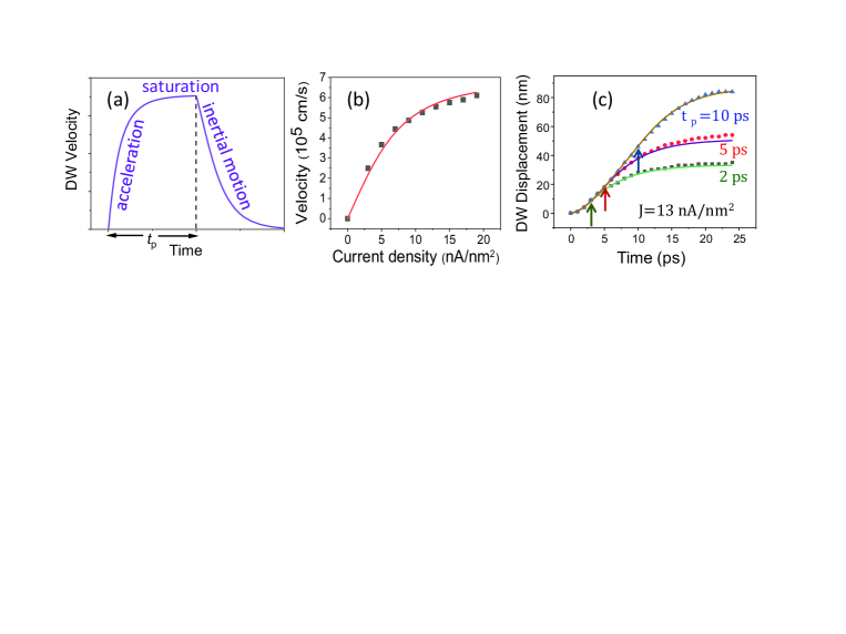
Figure 2: Comparison of the calculation results with the micromagnetic simulations in the deterministic transport (i.e., without thermal motions). (a) Characteristic evolution of the 90^∘ DW velocity in the thin-film AFM strip under a SOT pulse with duration $t_{p}$. (b) Steady-state DW velocity vs. the driving current density in the HM layer. (c) DW position as a function of time for different SOT pulse durations. The vertical arrows indicates the instants when the SOT is turned off. The driving current density $J$ is fixed at 13 nA/m². In (b,c), the data points are from micromagnetic simulations while the solid curves show the results from the model calculations. An excellent agreement is observed between them in both the steady-state and transient transport. The effect of coercivity is not considered here.

The calculations reveal the non-linear dependence of the DW velocity on the pulse intensity. As shown in Fig. 2(a), the AFM DW when subjected to an SOT pulse undergoes acceleration initially and then velocity saturation with the dissipation compensating the anti-damping SOT. Once the driving force is turn off, the inertial phase follows. Using the dimensional units, both the analytical solution and the results of the micromagnetic simulations are plotted in Fig. 2(b,c). A good agreement is observed between the two approaches in both the steady-state transport and the transient conditions with the inertial motion [Figs. 2(b) and 2(b), respectively], providing credence to the validity of the developed model. With the soliton ansatz verified, Eq. (9) can be expanded to account for the stochastic thermal motions in the DW dynamics at finite temperatures.

III.2 Effects of random thermal motion

The analysis of the thermal field influence on the DW transport supposes evaluation of thermal fluctuations $h_{\mathrm{th}}$ along the entire DW path. On the other hand, the perturbations away from the location of the wall texture are unlikely to affect the DW dynamics. The actual range of the AFM channel where the influence of random motions needs to be considered is the relatively narrow stretch corresponding to the wall texture (i.e., the DW width $\delta_{\mathrm{dw}}$). Thus the problem can be approximated to the analysis of the fluctuation effect in the finite volume of $V=A\times\delta_{\mathrm{dw}}$ associated with the soliton representation. Accordingly, the influence of the thermal field can be accounted for by conveniently adding of a randomly fluctuating field-like torque [i.e., $-\frac{\pi}{2\lambda}\frac{d}{dt}h_{\mathrm{th}}(t)$] to the current induced SOT $Q$ in the dynamical equation governing the soliton motion [see also Eq. (5)].

In describing the thermal field $h_{th}(t)$, the approximation based on a series of random step functions used commonly in the ferromagnetic systems cannot be applied here due to the explicit dependence on the time derivative Tsiantos2003 . As an alternative, a spectral representation is adopted in the form of a Fourier series expansion with random amplitudes Semenov2018 . This representation allows straightforward introduction of the upper and lower bounds in the noise spectrum by considering the auto-correlation time $\tau_{c}$ and the characteristic Néel-vector relaxation time $\tau_{m}$ (more precisely, the inverses $2\pi/\tau_{c}$ and $2\pi/\tau_{m}$, respectively). Furthermore, the fact that the lower truncation frequency $2\pi/\tau_{m}$ corresponds to the broadening of the AFM resonant frequency $\delta_{r}$ offers a physical ground for the discretization of the spectral domain in the comparable intervals. As the response of a damped Néel-vector motion becomes practically invariant to the perturbation frequency swing in the range of $\delta_{r}$ due to the broadening, the actual noise spectrum can be discretized likewise.

In other words, the AFM response to the thermal noise is virtually equivalent to a series of sinusoidal perturbations with random amplitudes and the frequencies $n\delta_{r}$ ($n=1,2,...,N$, where $N$ is given by $\tau_{m}/\tau_{c}$). The fluctuation dissipation theorem defines the amplitude of fluctuating field in the form Semenov2018 ,

$$h_{\mathrm{th}}(t)=\frac{\delta_{r}}{\omega_{r}}\left(\frac{2k_{B}T}{NV\left|K\right|}\right)^{1/2}\left(\sum_{n=1}^{N}\alpha_{n}\sin n\frac{\delta_{r}}{\omega_{r}}t+\sum_{n=1}^{N}\beta_{n}\cos n\frac{\delta_{r}}{\omega_{r}}t\right),$$ (16)

where $k_{B}T$ denotes the thermal energy, $n\frac{\delta_{r}}{\omega_{r}}t$ is actually $n\delta_{r}t$ in physical units, and $\frac{1}{2N}\sum_{n=1}^{N}\left\langle\alpha_{n}^{2}+\beta_{n}^{2}\right\rangle=1$. Note that the noise expression applies only for a duration up to $\tau_{m}$ in the time domain due to the relaxation. A time period longer than this interval requires repeated random selections. Equation (16) is clearly differentiable that can be directly incorporated into Eq. (9). The exact details of the noise model including a particular choice of the material parameters are not highly crucial in examining the possible electrical control in the thermally induced dispersion of the DW position.

Before accounting for the thermal component, Fig. 3 first examines the deterministic relation between the necessary SOT pulse strength and the duration for a desired travel distance $x_{0}$. The results are plotted in a normalized form in terms of $2\lambda t_{p}$ and $2\lambda x_{0}$ since it conveniently circumvents the explicit dependence on other physical parameters [see, for instance, Eqs. (10) and (14)]. The coercivity of $v_{c}=0.04$ is considered as well to reflect the conditions in the realistic structures [Eq. (15)]. As shown, both short and strong (red) as well as long and weak (blue) pulses can shift the DW by the same distance. The obtained relation serves as the guideline for the desired mean or average motion of the AFM DWs.

Once the influence of thermal fluctuations is accounted for, the DW dynamics deviates from the prescribed path [see the inset to Fig. 4(a)]. The resulting dispersion in the final position $x_{\mathrm{dw}}$ around $x_{0}$ can be calculated by numerically solving Eq. (9) in the presence of the random field-like torque $-\frac{\pi}{2\lambda}\frac{d}{dt}h_{\mathrm{th}}(t)$. A sufficiently large number of iterations $N_{i}$ are needed to ensure a statistically reliable outcome due to the stochastic nature of the calculation. For the numerical evaluation, the parameter values adopted earlier for Fig. 3 are also applied except $\lambda$, for which a slightly larger choice of 0.135 (thus, $\delta_{r}=2\pi\times$16.5 GHz) is used here. Likewise the magnitude of the auto-correlation time $\tau_{c}$ is treated empirically. Since our analysis is not significantly affected by the exact value of $\tau_{c}$ so long as it is sufficiently shorter than $\tau_{m}$, a small constant fraction ($\tau_{c}=0.01\tau_{m}$; $N=100$) is assumed for simplicity in Eq. (16). For a set of given conditions, the calculations are repeated 250 times ($=N_{i}$), each with an independently selected $h_{\mathrm{th}}(t)$ pattern randomly varying in time.

Figure 4(a) shows the typical probability distribution of the DW position for two SOT pulses at 300 K. While both pulses are designed to shift the DW by the same distance on average (see also two points marked in Fig. 3), the dispersion as the result of random thermal motion shows a significant difference. The short and strong pulse (red; $Q=0.015$) produces a much narrower distribution than the long and weak counterpart (blue; $Q=0.007$). It can be intuitively understood that the DW driven by a strong pulse is less likely to be influenced by the comparatively minor thermal fluctuations. At the same time, the DW is exposed to the random motions for a shorter duration in this case for it reaches the final destination quicker and then pinned by the coercivity. It is also interesting to note that the mean position $\left\langle x_{\mathrm{dw}}\right\rangle$ averaged over $N_{i}$ iterations is indeed given by $x_{0}$ as designed (from the deterministic analysis), with high accuracy. Since the pulse strength and duration can be controlled electrically, the probability distribution function in the DW position can be tuned likewise (i.e., narrower $\rightleftarrows$ broader). Combined with the structure utilizing the anisotropic magnetoresistance as shown in Fig. 1(a) Yu2018 ; Park2011 ; Lu2018 , it can be translated into a corresponding probabilistic distribution in the electrical output signal $-$ an essential component in the probabilistic computing or Bayesian learning. Finally, Fig. 4(b) plots the normalized standard deviation in the DW position $\Delta=\left\langle(x_{\mathrm{dw}}/\left\langle x_{\mathrm{dw}}\right\rangle-1)^{2}\right\rangle^{1/2}$ as a function of $Q$ for three average displacements. The observed large differences in $\Delta$ indicate that a broad range of probability distributions can be realized with a single AFM device. Moreover, the normalized deviation appears to be only weakly dependent on $x_{0}$ or $\left\langle x_{\mathrm{dw}}\right\rangle$ (thus, on the pulse duration $t_{p}$ for a given $Q$). Clearly, the determining factor is the pulse strength $Q$, to which $\Delta$ exhibits an inverse proportionality.

IV Summary

The fluctuating thermal fields in the antiferromagnets are identified as a potential mechanism to realize a probabilistic distribution in the electrical output signal, whose characteristic properties such as the standard deviation may also be tailored conveniently by electrical control. To this end, the dynamics of a 90^∘ DW driven by the current-induced SOT is theoretically examined at finite temperatures in a thin-film AFM structure. A soliton-type representation based on an energy balance equation is developed to describe the DW motion in combination with a stochastic thermal field model for AFM nano-particles. The calculation results clearly illustrate that both the average displacement of the DW position and its thermally induced dispersion can be modulated electrically by simply tuning the driving SOT strength and the duration. The corresponding probabilistic response in the electrical output signal via the magnetoresistance offers an effective means to realize the probability distribution functions that can be ”trained”. This unusual functionality may provide a key component in the emerging probabilistic computing and machine learning architectures.

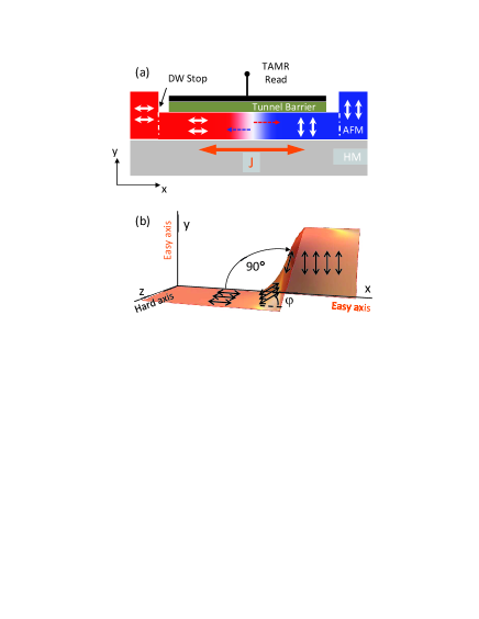
Figure 1: (a) Schematic illustration of the antiferromagnet-based DW device under consideration. The electric current $J$ through the heavy metal (HM) layer generates the spin current, providing the SOT to the AFM strip necessary for the DW motion. The 90^∘ DW can travel in either direction ($\pm x$) that is determined by the current flow in the HM layer. The shift in the DW position can be detected through the top contact either via the anisotropic magnetoresistance or its tunneling variety (TAMR) as shown. (b) Spin textures of the $90^{\circ}$ Néel DW with the heavy $z$-axis and the easy $x$- and $y$-axes.

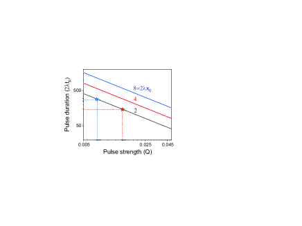
Figure 3: Calculated SOT pulse strength vs. the duration for three travel distances $x_{0}$ in the deterministic transport. The results are plotted in normalized units in terms of $2\lambda t_{p}$ and $2\lambda x_{0}$ to circumvent the explicit dependence on other physical parameters. The coercivity of $v_{c}=0.04$ is also included in the analysis. The blue and red points highlight two different conditions ($Q=$ 0.007 and 0.015, respectively) that shift the DW by the same distance.

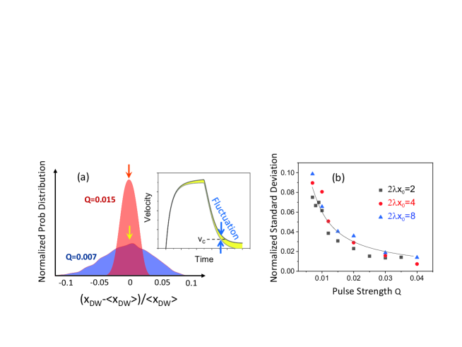
Figure 4: (a) Probability distribution of the DW position $x_{\mathrm{dw}}$ at 300 K calculated for two SOT pulses ($Q=0.015$ and $Q=0.007$ corresponding to the red and blue marks in Fig. 3, respectively). The horizontal axis shows the normalized deviation from the average position $\left\langle x_{\mathrm{dw}}\right\rangle$ which matches with $x_{0}$ from the deterministic analysis. The inset schematically illustrates the effect of random thermal fluctuations on the DW velocity. (b) Normalized standard deviation in the DW position as a function of the SOT strength for three average displacements $x_{0}$. The pulse duration corresponding to each $Q$ and $x_{0}$ can be found in Fig. 3. The solid curve represents a fit with an inverse proportionality $aQ^{-1}$ ($a=6\times 10^{-4}$). The coercivity ($v_{c}=0.04$) is accounted for in both (a) and (b).

- (1) O. Gomonay, T. Jungwirth, and J. Sinova, Concepts of antiferromagnetic spintronics, Phys. Status Solidi RRL 11, 1700022 (2017).
- (2) V. Baltz, A. Manchon, M. Tsoi, T. Moriyama, T. Ono, and Y. Tserkovnyak, Antiferromagnetic spintronics, Rev. Mod. Phys. 90, 015005 (2018).
- (3) K. M. D. Hals, Y. Tserkovnyak, and A. Brataas, Phenomenology of current-induced dynamics in antiferromagnets, Phys. Rev. Lett. 106, 107206 (2011).
- (4) A. C. Swaving and R. A. Duine, Current-induced torques in continuous antiferromagnetic textures, Phys. Rev. B 83, 054428 (2011).
- (5) E. G. Tveten, A. Qaiumzadeh, O. A. Tretiakov, and A. Brataas, Staggered dynamics in antiferromagnets by collective coordinates, Phys. Rev. Lett. 110, 127208 (2013).
- (6) S. K. Kim, Y. Tserkovnyak, and O. Tchernyshyov, Propulsion of a domain wall in an antiferromagnet by magnons, Phys. Rev. B 90, 104406 (2014).
- (7) E. G. Tveten, A. Qaiumzadeh, and A. Brataas, Antiferromagnetic domain wall motion induced by spin waves, Phys. Rev. Lett. 112, 147204 (2014).
- (8) A. Qaiumzadeh, L. A. Kristiansen, and A. Brataas, Controlling chiral domain walls in antiferromagnets using spin-wave helicity, Phys. Rev. B 97, 020402(R) (2018).
- (9) K. Pan, L. Xing, H. Y. Yuan, and W. Wang, Driving chiral domain walls in antiferromagnets using rotating magnetic fields, Phys. Rev. B 97, 184418 (2018).
- (10) D. R. Rodrigues, K. Everschor-Sitte, O. A. Tretiakov, J. Sinova, and Ar. Abanov, Spin texture motion in antiferromagnetic and ferromagnetic nanowires, Phys. Rev. B 95, 174408 (2017).
- (11) Y. Yamane, O. Gomonay, H. Velkov, and J. Sinova, Combined effect of magnetic field and charge current on antiferromagnetic domain-wall dynamics, Phys. Rev. B 96, 064408 (2017).
- (12) O. Gomonay, T. Jungwirth, and J. Sinova, High antiferromagnetic domain wall velocity induced by Néel spin-orbit torques, Phys. Rev. Lett. 117, 017202 (2016).
- (13) S. Yu. Bodnar, L. S̆mejkal, I. Turek, T. Jungwirth, O. Gomonay, J. Sinova, A. A. Sapozhnik, H.-J. Elmers, M. Kläui, and M. Jourdan, Writing and reading antiferromagnetic Mn2Au by Néel spin-orbit torques and large anisotropic magnetoresistance, Nat. Commun. 9, 348 (2018).
- (14) T. Shiino, S.-H. Oh, P. M. Haney, S.-W. Lee, G. Go, B.-G. Park, and K.-J. Lee, Antiferromagnetic domain wall motion driven by spin-orbit torques, Phys. Rev. Lett. 117, 087203 (2016).
- (15) B. G. Park, J. Wunderlich, X. Mart , V. Holý, Y. Kurosaki, M. Yamada, H. Yamamoto, A. Nishide, J. Hayakawa, H. Takahashi, A. B. Shick, and T. Jungwirth, A spin-valve-like magnetoresistance of an antiferromagnet-based tunnel junction, Nat. Mater. 10, 347 (2011).
- (16) D. Pinna, F. Abreu Araujo, J.-V. Kim, V. Cros, D. Querlioz, P. Bessiere, J. Droulez, and J. Grollier, Skyrmion gas manipulation for probabilistic computing, Phys. Rev. Applied 9, 064018 (2018).
- (17) Y. G. Semenov, X.-L. Li, X. Xu, and K. W. Kim, Helical waves in easy-plane antiferromagnets, Phys. Rev. B 96, 224432 (2017).
- (18) X. Li, X. Duan, Y. G. Semenov, and K. W. Kim, Electrical switching of antiferromagnets via strongly spin-orbit coupled materials, J. Appl. Phys. 121, 023907 (2017).
- (19) V. D. Tsiantos, T. Schrefl, W. Scholz, and J. Fidler, Thermal magnetization noise in submicrometer spin valve sensors, J. Appl. Phys. 93, 8576 (2003).
- (20) Y. G. Semenov, X. Xu, and K. W. Kim, Thermal fluctuations in antiferromagnetic nanostructures, arXiv:1806.11130v2.
- (21) Z. Yan, Z. Chen, M. Qin, X. Lu, X. Gao, and J. Liu, Brownian motion and entropic torque driven motion of domain walls in antiferromagnets, Phys. Rev. B 97, 054308 (2018).
- (22) C. Lu, B. Gao, H. Wang, W. Wang, S. Yuan, S. Dong, and J.-M. Liu, Revealing controllable anisotropic magnetoresistance in spin-orbit coupled antiferromagnet Sr2IrO4, Adv. Funct. Mater. 28, 1706589 (2018).