A variational approach to the sum splitting scheme

Abstract.

Nonlinear parabolic equations are frequently encountered in applications and efficient approximating techniques for their solution are of great importance. In order to provide an effective scheme for the temporal approximation of such equations, we present a sum splitting scheme that comes with a straight forward parallelization strategy. The convergence analysis is carried out in a variational framework that allows for a general setting and, in particular, nontrivial temporal coefficients. The aim of this work is to illustrate the significant advantages of a variational framework for operator splittings and use this to extend semigroup based theory for this type of schemes.

1. Introduction

Nonlinear parabolic equations, which we state as abstract evolution equation of the form

(1.1) $$u^{\prime}(t)+A(t)u(t)=f(t),\quad t\in(0,T)\quad\text{and}\quad u(0)=u_{0},$$

are frequently encountered in applications appearing in physics, chemistry and biology; see [2] and [28, Section 1.3]. A few standard examples of the diffusion operator $A(t)v$ are

(1.2) $$-\nabla\cdot\bigl{(}\alpha(t)|\nabla v|^{p-2}\nabla v\bigr{)},\quad-\Delta(\alpha(t)|v|^{p-2}v\bigr{)}\quad\text{and}\quad-\sum_{i=1}^{d}D_{i}\bigl{(}\alpha(t)|D_{i}v|^{p-2}D_{i}v\bigr{)}.$$

Here, the first and second operator is referred to as the $p$-Laplacian and the porous medium operator, respectively.

Due to the problems’ significance, effective techniques for their approximations become crucial. As we consider parabolic equations, for stability reasons the temporal approximation schemes need to be implicit. For equations which in addition are given in several spatial dimensions the resulting spatial and temporal approximation schemes require large scale computations. This typically demands implementations in parallel on a distributed hardware. One possibility to design temporal approximation schemes that can directly be implemented in a parallel fashion is to utilize operator splitting; see, e.g., [19] for an introduction. Note that the solutions of nonlinear parabolic problems typically lack high-order spatial and temporal regularity. Thus, there is little use to consider high-order time integrators.

In order to illustrate the splitting concept, consider the simplest implicit scheme, namely, the backward Euler method. For $N$ temporal steps, a step size $k=T/N$ and the starting value $\mathbf{U}^{0}=u^{0}$ the backward Euler approximation $\mathbf{U}^{n}$ of $u(nk)$ is given by the recursion

$$\frac{1}{k}(\mathbf{U}^{n}-\mathbf{U}^{n-1})+k\mathbf{A}^{n}\mathbf{U}^{n}=\mathbf{f}^{n},\quad n\in\{1,\ldots,N\},$$

where $(\mathbf{A}^{n})_{n}$ and $(\mathbf{f}^{n})_{n}$ are suitable approximations for $A$ and $f$, respectively. Assuming that the nonlinear resolvent of $\mathbf{A}^{n}$ exists, we find the reformulation

$$\mathbf{U}^{n}=(I+k\mathbf{A}^{n})^{-1}\bigl{(}\mathbf{U}^{n-1}+k\mathbf{f}^{n}),\quad n\in\{1,\ldots,N\}.$$

To implement one step of the backward Euler scheme in parallel, we split the Euler step into $s$ independently solvable problems. To this end, we decompose $\mathbf{A}^{n}$ and $\mathbf{f}^{n}$ as

(1.3) $$\mathbf{A}^{n}=\sum_{\ell=1}^{s}\mathbf{A}^{n}_{\ell}\quad\text{and}\quad\mathbf{f}^{n}=\sum_{\ell=1}^{s}\mathbf{f}^{n}_{\ell},\quad n\in\{1,\ldots,N\}.$$

With this abstract operator splitting, one can design various temporal approximation schemes. Two possibilities to split one single Euler step are given by formally multiplying or adding the operators $(I+k\mathbf{A}^{n}_{\ell})^{-1}$, $\ell\in\{1,\dots,s\}$. A composition of such fractional step operators yields the Lie splitting scheme

$$(I+k\mathbf{A}^{n})^{-1}\approx\prod_{\ell=1}^{s}(I+k\mathbf{A}^{n}_{\ell})^{-1}.$$

Thus, we obtain $s$ possibly easier subproblems that are solved after each other. For a straightforward parallelization it is more convenient to choose a splitting, where the single steps can be computed at the same time. The sum splitting

$$(I+k\mathbf{A}^{n})^{-1}\approx\frac{1}{s}\sum_{\ell=1}^{s}(I+ks\mathbf{A}^{n}_{\ell})^{-1}$$

offers this crucial advantage. The $s$ fractional steps are solved at the same time and their average is used as an approximation.

The decomposition (1.3) can be utilized in many different ways. A first possible application is a source term splitting, where the high-order terms are split from the low-order terms. For example a source term splitting of the reaction-diffusion equation governed by $A(t)v=-\nabla\cdot\bigl{(}\alpha(t)\nabla v\bigr{)}+p(t,v)$ would have the form

$$\mathbf{A}_{1}^{n}v=-\nabla\cdot\bigl{(}\alpha(nk)\nabla v\bigr{)}\quad\text{and}\quad\mathbf{A}_{2}^{n}v=p(nk,v).$$

Here, the actions of $(I+k\mathbf{A}^{n}_{1})^{-1}$ can be evaluated by a standard fast linear elliptic solver and the actions of the nonlinear resolvent $(I+k\mathbf{A}^{n}_{2})^{-1}$ can often be expressed in a closed form. Examples of studies dealing with various source term splittings can be found in [3, 18, 20, 7].

Another possibility is a dimension splitting, where each spatial derivative is considered as a separate differential operator. For example, the dimension splitting of the nonlinear porous medium operator and the third operator in (1.2) are given by

$$\mathbf{A}_{\ell}^{n}v=-D_{\ell\ell}\bigl{(}\alpha(nk)|v|^{p-2}v\bigr{)}\quad\text{and}\quad\mathbf{A}_{\ell}^{n}v=-D_{\ell}\bigl{(}\alpha(nk)|D_{\ell}v|^{p-2}D_{\ell}v\bigr{)},$$

respectively. This splitting yields that the action of each nonlinear resolvent $(I+k\mathbf{A}^{n}_{\ell})^{-1}$ can be separated into lower-dimensional subproblems that can be solved on their own. Note that the $p$-Laplacian lacks a natural dimension splitting. Examples of convergence results for the dimension splitting of the third equation in (1.2) can be found in [26], where the Lie scheme is used, and in [17], where the sum, Lie and Peaceman–Rachford schemes are considered for the autonomous case.

A limitation of the dimension splitting approach is the rather large need of communication between the subproblems, which can impede an effective distributed implementation. Dimension splitting is also quite restrictive in terms of the spatial domains that can be considered. A modern alternative to dimension splitting, which is applicable to a very general class of spatial domains, is the domain decomposition based splitting. Here, the subproblems are given on $s$ spatial subdomains that share a small overlap. As an example consider the three nonlinear diffusion operators (1.2) and introduce a partition of unity $(\chi_{\ell})_{\ell=1}^{s}$, where each weight function $\chi_{\ell}$ vanishes outside its corresponding spatial subdomain. The domain decompositions $\mathbf{A}_{\ell}^{n}v$ are then

$$-\nabla\cdot\bigl{(}\chi_{\ell}\alpha(nk)|\nabla v|^{p-2}\nabla v\bigr{)},\quad-\Delta\bigl{(}\chi_{\ell}\alpha(nk)|v|^{p-2}v\bigr{)}$$

$$\quad\text{and}\quad-\sum_{i=1}^{d}D_{i}\bigl{(}\chi_{\ell}\alpha(nk)|D_{i}v|^{p-2}D_{i}v\bigr{)},$$

respectively. This approach is well suited for a parallel computation, as the actions of $(I+k\mathbf{A}^{n}_{\ell})^{-1}$ can be solved independently of each other and the communication required is small, due to the small overlaps between the subdomains. Studies regarding domain decomposition based splittings applied to linear and autonomous parabolic equations include [3, 16, 23, 27]. Convergence for the Lie and sum splittings are given in [8] for the autonomous $p$-Laplace and porous medium equations.

Operator splitting schemes are typically analyzed in a semigroup framework, which yields convergence for a wide range of temporal approximation schemes, including the Lie and sum schemes; see [4] for more details on the solution concept. However, there does not seem to be a straightforward way to extend the semigroup based convergence analysis to nonautonomous evolution equations. Furthermore, the semigroup framework requires some additional regularity conditions to relate the intersection of the domains $D(A_{\ell})$, $\ell\in\{1,\dots,s\}$, with the domain $D(A)$ of the full operator. The latter, e.g., implies restrictions on the domain decomposition of the $p$-Laplace equation [8, Section 6].

In a variational setting this problem is avoided in a natural way while at the same time the analysis of nonautonomous problems is accessible. Also the structure of this approach is well suited to include a Galerkin scheme and therefore, in particular, the finite element method. However, the analysis typically needs to be tailored for each method. The variational setting is a standard tool for existence theories [9, 25, 30] and has been used in several works in the context of “unsplit” time integrators [10, 11, 12, 13]. However, in the context of temporal splitting schemes for nonlinear parabolic equations the only variational studies that we are aware of is [26]. Here, a variational analysis is employed when proving the convergence of the Lie scheme applied to nonautonomous evolution equations and, as already stated, is applied to the dimension splitting of the third equation in (1.2).

Hence, the aim of this paper is threefold. Firstly, we aim to generalize the previous semigroup based analysis for the sum scheme to nonautonomous evolution equations without any implicit regularity assumptions. The latter generalization will be applicable to splittings of reaction-diffusion, dimension and domain decomposition type. Secondly, we intend to extend the abstract variational convergence results for the Lie scheme to the sum splitting scheme. As this requires a tailored convergence proof, it is not a trivial implication. Thirdly, we also strive to illustrate the advantages of a variational approach in the context of splitting analyses.

This paper is organized as follows: In Section 2, we state the exact assumptions that are needed on the abstract variational framework considered in the paper. This section also contains an example that shows that the relevant application of domain decomposition integrators for the $p$-Laplacian operator fits into our abstract framework. This in mind, we prove the well-posedness of the sum scheme, as well as suitable a priori bounds in Section 3. The main convergence results are proven in Section 4; see Theorem 4.5 and Theorem 4.6.

2. Abstract setting

In this section, we introduce an abstract setting for the convergence analysis of the sum splitting scheme. We begin by presenting the exact assumptions made on the data and present the temporal discretization of the problem. This at hand, we can state the scheme that we will work with in this paper. The section ends with a more concrete setting that exemplifies the abstract framework.

Assumption 1.

Let $(H,(\cdot,\cdot)_{H},\|\cdot\|_{H})$ be a real, separable Hilbert space and let $(V,\|\cdot\|_{V})$ be a real, separable, reflexive Banach space such that $V$ is continuously and densely embedded into $H$. Further, there exist a seminorm $|\cdot|_{V}$ on $V$ and $c_{V}\in(0,\infty)$ such that $\|\cdot\|_{V}\leq c_{V}\big{(}\|\cdot\|_{H}+|\cdot|_{V}\big{)}$ is fulfilled.

Furthermore, for $s\in\mathbb{N}$ let $(V_{\ell},\|\cdot\|_{V_{\ell}})$, $\ell\in\{1,\dots,s\}$, be real reflexive Banach spaces that are continuously and densely embedded into $H$, fulfill $\bigcap_{\ell=1}^{s}V_{\ell}=V$ and $\sum_{\ell=1}^{s}\|\cdot\|_{V_{\ell}}$ is equivalent to $\|\cdot\|_{V}$. For every $\ell\in\{1,\dots,s\}$, there exists a seminorm $|\cdot|_{V_{\ell}}$ and $c_{V_{\ell}}\in(0,\infty)$ such that $\|\cdot\|_{V_{\ell}}\leq c_{V_{\ell}}\big{(}\|\cdot\|_{H}+|\cdot|_{V_{\ell}}\big{)}$ and $\sum_{\ell=1}^{s}|\cdot|_{V_{\ell}}$ is equivalent to $|\cdot|_{V}$.

Identifying $H$ with its dual space $H^{*}$, we obtain the Gelfand triples

$$V\overset{d}{\hookrightarrow}H\cong H^{*}\overset{d}{\hookrightarrow}V^{*}\quad\text{and}\quad V_{\ell}\overset{d}{\hookrightarrow}H\cong H^{*}\overset{d}{\hookrightarrow}V^{*}_{\ell},\quad\ell\in\{1,\dots,s\}.$$

The next assumption states the properties of the differential operator that are of importance.

Assumption 2.

Let $H$ and $V$ be given as stated in Assumption 1. Furthermore, for $T>0$ and $p>1$, let $\{A(t)\}_{t\in[0,T]}$ be a family of operators such that $A(t)\colon V\to V^{*}$ satisfy the following conditions:

• The mapping $Av\colon[0,T]\to V^{*}$, $v\in V$, given by $t\mapsto A(t)v$ is continuous.

• The operator $A(t)\colon V\to V^{*}$, $t\in[0,T]$, is radially continuous, i.e., the mapping $\tau\mapsto\langle A(t)(u+\tau v),w\rangle_{V^{*}\times V}$ is continuous on $[0,1]$ for $u,v,w\in V$.

• The operator $A(t)\colon V\to V^{*}$, $t\in[0,T]$, fulfills a monotonicity condition such that there exists $\eta\geq 0$ with

  $$\langle A(t)v-A(t)w,v-w\rangle_{V^{*}\times V}\geq\eta|v-w|_{V}^{p},\quad v,w\in V.$$

• The operator $A(t)\colon V\to V^{*}$, $t\in[0,T]$, is uniformly bounded such that there exists $\beta>0$ with

  $$\|A(t)v\|_{V^{*}}\leq\beta\big{(}1+\|v\|_{V}^{p-1}\big{)},\quad v\in V.$$

• The operator $A(t)\colon V\to V^{*}$, $t\in[0,T]$, fulfills a coercivity condition such that there exist $\mu>0$ and $\lambda\geq 0$ with

  $$\langle A(t)v,v\rangle_{V^{*}\times V}+\lambda\geq\mu|v|_{V}^{p},\quad v\in V.$$

Now, we can combine Assumption 1 and Assumption 2 to state a decomposition of the operator family $\{A(t)\}_{t\in[0,T]}$ that we employ in the analysis of the sum splitting scheme.

Assumption 3.

For $s\in\mathbb{N}$ let $H$, $V$ and $V_{\ell}$, $\ell\in\{1,\dots,s\}$, fulfill Assumption 1. For $p>1$ and $T>0$ let the operator family $\{A(t)\}_{t\in[0,T]}$ be given such that it fulfills Assumption 2. Further, let $\{A_{\ell}(t)\}_{t\in[0,T]}$, $\ell\in\{1,\dots,s\}$, be given such that $A_{\ell}(t)\colon V_{\ell}\to V_{\ell}^{*}$ fulfills Assumption 2, with $V$ replaced by $V_{\ell}$ for every $\ell\in\{1,\dots,s\}$. Moreover, let the sum property

$$\sum_{\ell=1}^{s}A_{\ell}(t)v=A(t)v\quad\text{in }V^{*},\quad t\in[0,T],v\in V$$

be fulfilled.

Remark 2.1.

Note that the optimal coefficients $\beta,\eta,\lambda,\mu$ for the operator families $\{A(t)\}_{t\in[0,T]}$, $\{A_{\ell}(t)\}_{t\in[0,T]}$, $\ell\in\{1,\dots,s\}$, of operators do not necessarily have to be the same. For the sake of simplicity, we assume that these coefficients coincide.

We also consider the differential operators of Assumption 3 as Nemytskii operators acting on spaces of Bochner integrable functions. For an introduction to Bochner integrable functions we refer the reader to [5, Chapter II] or [24, Section 4.2]. Some properties of such Nemytskii operators are collected in the next lemma. The proofs can be found in [9, Lemma 8.4.4].

Lemma 2.2.

For $p>1$, $q=\frac{p}{p-1}$ and $T>0$ let $\{A(t)\}_{t\in[0,T]}$ fulfill Assumption 2. Then the operator $(Av)(t)=A(t)v(t)$ maps $L^{p}(0,T;V)$ into $L^{q}(0,T;V^{*})$. The operator is radially continuous, i.e., the mapping $\tau\mapsto\langle A(u+\tau v),w\rangle_{L^{q}(0,T;V^{*})\times L^{p}(0,T;V)}$ is continuous on $[0,1]$ for all $u,v,w\in L^{p}(0,T;V)$. Furthermore, it fulfills a monotonicity, a boundedness and a coercivity condition such that

$$\langle Av-Aw,v-w\rangle_{L^{q}(0,T;V^{*})\times L^{p}(0,T;V)}\geq\eta\int_{0}^{T}|v(t)-w(t)|_{V}^{p}\,\mathrm{d}t,$$

$$\|Av\|_{L^{q}(0,T;V^{*})}\leq\beta\big{(}T^{\frac{1}{q}}+\|v\|_{L^{p}(0,T;V)}^{p-1}\big{)},$$

$$\langle Av,v\rangle_{L^{q}(0,T;V^{*})\times L^{p}(0,T;V)}+\lambda T\geq\mu\int_{0}^{T}|v(t)|_{V}^{p}\,\mathrm{d}t$$

for all $v,w\in L^{p}(0,T;V)$.

The Nemytskii operator of $\{A_{\ell}(t)\}_{t\in[0,T]}$, $\ell\in\{1,\dots,s\}$, as introduced in Assumption 3 also fulfills the same bounds with $V$ replaced by $V_{\ell}$. To make our setting complete, it remains to state the assumptions on $f$.

Assumption 4.

Let $V$ and $V_{\ell}$, $\ell\in\{1,\dots,s\}$, fulfill Assumption 1. Let $p$ be the same value as in Assumption 2 and $q=\frac{p}{p-1}$. Further, let $f$ be in $L^{q}(0,T;V^{*})$. Assume that there exist functions $f_{\ell}\in L^{q}(0,T;V^{*}_{\ell})$, $\ell\in\{1,\dots,s\}$, such that

$$\sum_{\ell=1}^{s}f_{\ell}(t)=f(t)\text{ in }V^{*}\quad\text{and}\quad\|f_{\ell}(t)\|_{V_{\ell}^{*}}\leq\|f(t)\|_{V^{*}},\quad\text{ a.e. }t\in(0,T).$$

Note that this assumption can be generalized to functions $f\in L^{q}(0,T;V^{*})+L^{2}(0,T;H)$, compare, for example, [11, 13]. In order to keep the presentation more simple, we only consider the smaller space $L^{q}(0,T;V^{*})$.

We can now state the abstract evolution equation that we want to consider. In the following, let $\{A(t)\}_{t\in[0,T]}$ be as stated in Assumption 3, let $f$ fulfill Assumption 4 and let $u_{0}\in H$ be given. It is our overall goal to find an approximation to the solution $u$ of

(2.1) $$\begin{split}\begin{cases}u^{\prime}+Au=f\quad&\text{in }L^{q}(0,T;V^{*}),\\ u(0)=u_{0}&\text{in }H.\end{cases}\end{split}$$

This evolution equation is uniquely solvable in a variational sense with a solution $u$ in $\mathcal{W}^{p}(0,T)\hookrightarrow C([0,T];H)$, where

$$\mathcal{W}^{p}(0,T)=\{v\in L^{p}(0,T;V):v^{\prime}\in L^{q}(0,T;V^{*})\};$$

see [22, Section 2.7] and [25, Chapter 7–8] for further details. In the following analysis, we employ the sum splitting in order to obtain a temporal discretization of (2.1). To this end, we consider an equidistant grid on $[0,T]$, where $N\in\mathbb{N}$, $k=\frac{T}{N}$ and $t_{n}=nk$ for $n\in\{0,\dots,N\}$. For $\ell\in\{1,\dots,s\}$ and $n\in\{1,\dots,N\}$ we introduce

(2.2) $$\mathbf{A}_{\ell}^{n}=A_{\ell}(t_{n})\quad\text{and}\quad\mathbf{f}_{\ell}^{n}=\frac{1}{k}\int_{t_{n-1}}^{t_{n}}f_{\ell}(t)\,\mathrm{d}t.$$

We use this to construct an approximation $\mathbf{U}^{n}\approx u(t_{n})$ of the solution $u$ of (2.1) for $n\in\{0,\dots,N\}$. This approximation is given through a recursion

(2.3) $$\begin{cases}\frac{\mathbf{U}_{\ell}^{n}-\mathbf{U}^{n-1}}{k}+s\mathbf{A}_{\ell}^{n}\mathbf{U}_{\ell}^{n}=s\mathbf{f}_{\ell}^{n}\quad&\text{in }V_{\ell}^{*},\quad\ell\in\{1,\dots,s\},\\ \mathbf{U}^{n}=\frac{1}{s}\sum_{\ell=1}^{s}\mathbf{U}_{\ell}^{n}\quad&\text{in }H\end{cases}$$

for $n\in\{1,\dots,N\}$ with $\mathbf{U}^{0}=u_{0}$.

Example 2.3.

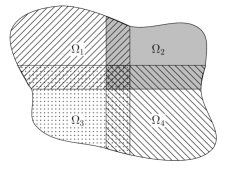
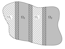
Figure 1. Examples of overlapping domains $\{\Omega_{\ell}\}_{\ell=1}^{s}$ of $\Omega\subset\mathbb{R}^{2}$, with $s=4$ subdomains (left) and $s=2$ subdomains that are further decomposed into disjoint sets (right).

A useful example that fits into our abstract setting is to approximate the solution of the parabolic $p$-Laplace equation. Let $\Omega\subset\mathbb{R}^{d}$, $d\geq 1$, be given, where $\Omega$ is a bounded domain and the boundary $\partial\Omega$ is Lipschitz. For $p\geq 2$ we consider the problem

(2.4) $$\begin{cases}u_{t}(t,x)-\nabla\cdot(\alpha(t)|\nabla u(t,x)|^{p-2}\nabla u(t,x))=g(t,x),\quad&(t,x)\in(0,T)\times\Omega,\\ \alpha(t)|\nabla u(t,x)|^{p-2}\nabla u(t,x)\cdot n=0,&(t,x)\in(0,T)\times\partial\Omega,\\ u(0,x)=u_{0}(x),&x\in\Omega,\end{cases}$$

where $n$ denotes outer pointing normal vector. The function $\alpha\colon[0,T]\to\mathbb{R}$ is an element of $C([0,T])$, $u_{0}\in L^{2}(\Omega)$ and $g\colon(0,T)\times\Omega\to\mathbb{R}$ is a suitably chosen integrable function that we explain in more detail at a later point. Applications for this type of equation can be found in [2]. Our theory allows to solve (2.4) with the help of a domain decomposition scheme. A similar setting can be found in [16] for $p=2$. The case $p\geq 2$ for an autonomous problem with a more restrictive domain decomposition around the boundary can be found in [8, Section 6]. For $s\in\mathbb{N}$ let $\{\Omega_{\ell}\}_{\ell=1}^{s}$ be a family of overlapping subsets of $\Omega$ such that $\bigcup_{\ell=1}^{s}\Omega_{\ell}=\Omega$ is fulfilled. Furthermore, let each $\Omega_{\ell}$, $\ell\in\{1,\dots,s\}$, be either an open connected set with a Lipschitz boundary or a union of pairwise disjoint open, connected sets $\Omega_{\ell,i}$ such that $\bigcup_{i=1}^{r}\Omega_{\ell,i}=\Omega_{\ell}$ and $\Omega_{\ell,i}$ has a Lipschitz boundary for every $\ell\in\{1,\dots,s\}$ and $i\in\{1,\dots,r\}$; see Fig. 1.

On these subdomains let the partition of unity $\{\chi_{\ell}\}_{\ell=1}^{s}\subset W^{1,\infty}(\Omega)$ be given such that

$$\chi_{\ell}(x)>0\text{ for all }x\in\Omega_{\ell},\quad\chi_{\ell}(x)=0\text{ for all }x\in\Omega\setminus\Omega_{\ell},\quad\sum_{\ell=1}^{s}\chi_{\ell}=1$$

for $\ell\in\{1,\dots,s\}$. For such a function $\chi_{\ell}$, $\ell\in\{1,\dots,s\}$, the weighted Lebesgue space $L^{p}(\Omega_{\ell},\chi_{\ell})^{d}$ consists of all measurable functions $v=(v_{1},\dots,v_{d})\colon\Omega_{\ell}\to\mathbb{R}^{d}$ such that

$$\|(v_{1},\ldots,v_{d})\|_{L^{p}(\Omega_{\ell},\chi_{\ell})^{d}}=\Big{(}\int_{\Omega_{\ell}}\chi_{\ell}|(v_{1},\ldots,v_{d})|^{p}\,\mathrm{d}x\Big{)}^{\frac{1}{p}}$$

is finite. The space $L^{p}(\Omega_{\ell},\chi_{\ell})^{d}$ is a reflexive Banach space; see [6, Chapter 1] and [1, Theorem 1.23]. Note that $L^{p}(\Omega_{\ell})^{d}$ is a subspace of $L^{p}(\Omega_{\ell},\chi_{\ell})^{d}$ and it holds true that $\|v\|_{L^{p}(\Omega_{\ell},\chi_{\ell})^{d}}\leq\|v\|_{L^{p}(\Omega_{\ell})^{d}}$ for every $v\in L^{p}(\Omega_{\ell})^{d}$.

For $\left(H,(\cdot,\cdot)_{H},\|\cdot\|_{H}\right)$ we use $L^{2}(\Omega)$ the space of square integrable functions on $\Omega$ with the usual norm and inner product. The energetic spaces $V$ and $V_{\ell}$ are then given as

$$V =\Bigl{\{}u\in H:\text{ there exists a }v=(v_{1},\dots,v_{d})\in L^{p}(\Omega)^{d}\text{ such that }$$

$$\qquad\qquad\int_{\Omega}uD_{i}\varphi\,\mathrm{d}x=\int_{\Omega}v_{i}\varphi\,\mathrm{d}x\quad\text{for all }\varphi\in C^{\infty}_{0}(\Omega),\ i=1,\dots,d\Bigr{\}}=W_{0}^{1,p}(\Omega)$$

and

$$V_{\ell} =\Bigl{\{}u\in H:\text{ there exists a }v=(v_{1},\dots,v_{d})\in L^{p}(\Omega_{\ell},\chi_{\ell})^{d}\text{ such that }$$

$$\qquad\qquad\int_{\Omega}uD_{i}(\chi_{\ell}\varphi)\,\mathrm{d}x=\int_{\Omega_{\ell}}v_{i}\chi_{\ell}\varphi\,\mathrm{d}x\quad\text{for all }\varphi\in C^{\infty}_{0}(\Omega),\ i=1,\dots,d\Bigr{\}},$$

which are equipped with the norms

$$\|\cdot\|_{V}=\|\cdot\|_{H}+\|\nabla\cdot\|_{L^{p}(\Omega)^{d}}\quad\text{and}\quad\|\cdot\|_{V_{\ell}}=\|\cdot\|_{H}+\|\nabla\cdot\|_{L^{p}(\Omega_{\ell},\chi_{\ell})^{d}}.$$

For $t\in[0,T]$ we introduce the operator $A(t)\colon V\to V^{*}$

$$\langle A(t)u,v\rangle_{V^{*}\times V}=\int_{\Omega}\alpha(t)|\nabla u|^{p-2}\nabla u\cdot\nabla v\,\mathrm{d}x,\quad u,v\in V.$$

Together with the partition of unity we define the decomposed energetic operators $A_{\ell}(t)\colon V_{\ell}\to V^{*}_{\ell}$, $\ell\in\{1,\dots,s\}$,

$$\langle A_{\ell}(t)u,v\rangle_{V_{\ell}^{*}\times V_{\ell}}=\int_{\Omega_{\ell}}\chi_{\ell}\alpha(t)|\nabla u|^{p-2}\nabla u\cdot\nabla v\,\mathrm{d}x,\quad u,v\in V_{\ell},\quad t\in[0,T].$$

It is also possible to allow for more general coefficients $\alpha\colon[0,T]\times\overline{\Omega}\times\mathbb{R}^{d}\to\mathbb{R}^{d}$ where $\alpha(t,\cdot,\cdot)$ fulfills the condition stated in [8, Assumption 3].

We assume that for $g\colon(0,T)\times\Omega\to\mathbb{R}$ the abstract function $[f(t)](x)=g(t,x)$, $(t,x)\in(0,T)\times\Omega$, is an element of $L^{q}(0,T;V^{*})$. We exploit that $f(t)\in V^{*}$, $t\in(0,T)$, can be represented by

$$\langle f(t),v\rangle_{V^{*}\times V}=\int_{\Omega}f^{0}(t)v\,\mathrm{d}x+\sum_{i=1}^{d}\int_{\Omega}f^{i}(t)D_{i}v\,\mathrm{d}x,\quad v\in V$$

where $f^{i}(t)\in L^{q}(\Omega)$ for $i\in\{0,\dots,d\}$. These functions are not necessarily unique unless we exchange $V=W^{1,p}(\Omega)$ by $V=W_{0}^{1,p}(\Omega)$, compare [21, Theorem 10.41, Corollary 10.49]. This in mind, we introduce $f_{\ell}(t)$ for a.e. $t\in(0,T)$ as

$$\langle f_{\ell}(t),v\rangle_{V_{\ell}^{*}\times V_{\ell}}=\int_{\Omega}\chi_{\ell}f^{0}(t)v\,\mathrm{d}x+\sum_{i=1}^{d}\int_{\Omega}\chi_{\ell}f^{i}(t)D_{i}v\,\mathrm{d}x,\quad v\in V_{\ell}.$$

Note that in this type of setting, we can also consider homogeniuous Direchlet boundary conditions in (2.4). Then an additional condition on the partition of unity becomes necessary. In this case, we have to make the further assumption that for every function $\chi_{\ell}$ there exists $\varepsilon_{0}>0$ such that for all $\varepsilon\in(0,\varepsilon_{0})$

$$\Omega_{\ell}^{\varepsilon}=\{x\in\Omega_{\ell}:\chi_{\ell}(x)\geq\varepsilon\}$$

is a Lipschitz domain.

Further examples that fit our framework are a domain decomposition scheme for the porous medium equation as presented in [8, Section 7] or a source term splitting as in [7, Section 3.3]. An application to the third equation of (1.2) is presented in [26]. Numerical experiments for this equation and the $p$-Laplace equation can be found in [8] and [17], respectively.

3. Solvability and a priori bounds for the discrete scheme

The abstract setting from the previous section in mind we are now well-prepared to state some properties of the solution of the numerical scheme (2.3). Since the scheme is implicit, we start to verify that (2.3) is uniquely solvable. Once this is at hand, we can provide a priori bounds of the solution. These bounds are a crucial part of the further analysis and allow for the convergence analysis in Section 4

Lemma 3.1.

Let Assumptions 3 and 4 be fulfilled. Then the semidiscrete problem (2.3) is uniquely solvable.

Proof.

In order to prove the existence of the elements $(\mathbf{U}_{\ell}^{i})_{i\in\{0,\dots,N\}}$, $\ell\in\{1,\dots,s\}$, that fulfill (2.3), we argue inductively. Assuming that for $i\in\{1,\dots,N\}$ the previous elements $(\mathbf{U}_{\ell}^{j})_{j\in\{0,\dots,i-1\}}$, $\ell\in\{1,\dots,s\}$, exist in the corresponding spaces, we prove the existence of $\mathbf{U}_{\ell}^{i}\in V_{\ell}$ for every $\ell\in\{1,\dots,s\}$. The operator $I+sk\mathbf{A}_{\ell}^{i}$, $\ell\in\{1,\dots,s\}$, is strictly monotone due to (3) of Assumption 2, i.e., it holds true that

$$\langle(I+sk\mathbf{A}_{\ell}^{i})v-(I+sk\mathbf{A}_{\ell}^{i})w,v-w\rangle_{V_{\ell}^{*}\times V_{\ell}}>0,\quad v,w\in V_{\ell}\text{ with }v\neq w$$

for every $\ell\in\{1,\dots,s\}$. Furthermore, $I+sk\mathbf{A}_{\ell}^{i}$ is radially continuous as $A_{\ell}(t)$, $\ell\in\{1,\dots,s\}$, is radially continuous for every $t\in[0,T]$. It remains to verify that the operator is coercive. Using (5) of Assumption 2 and the norm bound of Assumption 1, it follows

$$\frac{\langle\big{(}I+sk\mathbf{A}_{\ell}^{i}\big{)}v,v\rangle_{V_{\ell}^{*}\times V_{\ell}}}{\|v\|_{V_{\ell}}} \geq\frac{\|v\|_{H}^{2}+sk\mu|v|_{V_{\ell}}^{p}-sk\lambda}{c_{V_{\ell}}\big{(}\|v\|_{H}+|v|_{V_{\ell}}\big{)}}$$

$$\geq\frac{\min(1,sk\mu)}{c_{V_{\ell}}}\cdot\frac{\|v\|_{H}^{2}+|v|_{V_{\ell}}^{p}}{\|v\|_{H}+|v|_{V_{\ell}}}-\frac{sk\lambda}{c_{V_{\ell}}\big{(}\|v\|_{H}+|v|_{V_{\ell}}\big{)}}\to\infty$$

as $\|v\|_{V_{\ell}}\to\infty$ for $v\in V_{\ell}$ and $\ell\in\{1,\dots,s\}$. Thus, for $\mathbf{U}^{i-1}=\frac{1}{s}\sum_{\ell=1}^{s}\mathbf{U}_{\ell}^{i-1}\in H$, there exists a unique solution $\mathbf{U}_{\ell}^{i}\in V_{\ell}$ of

(3.1) $$\big{(}I+sk\mathbf{A}_{\ell}^{i}\big{)}\mathbf{U}_{\ell}^{i}=sk\mathbf{f}_{\ell}^{i}+\mathbf{U}^{i-1}$$

for every $\ell\in\{1,\dots,s\}$ due Browder–Minty theorem; see [25, Theorem 2.14] for further details. ∎

We can now turn our attention to the a priori bounds.

Lemma 3.2.

Let Assumptions 3 and 4 be fulfilled. Then for the unique solution of (2.3) there exist constants $M,M^{\prime}<\infty$ such that for every step size $k=\frac{T}{N}$ the a priori bounds

(3.2) $$\begin{split}\max_{n\in\{1,\dots,N\}}\Big{(}\frac{1}{s}\sum_{\ell=1}^{s}\|\mathbf{U}_{\ell}^{n}\|^{2}_{H}\Big{)}+\frac{1}{s}\sum_{i=1}^{N}\sum_{\ell=1}^{s}\|\mathbf{U}_{\ell}^{i}-\mathbf{U}^{i-1}\|^{2}_{H}+k\sum_{i=1}^{N}\sum_{\ell=1}^{s}\|\mathbf{U}_{\ell}^{i}\|_{V_{\ell}}^{p}\leq M\end{split}$$

and

(3.3) $$\frac{1}{k}\sum_{i=1}^{N}\Big{\|}\frac{\mathbf{U}^{i}-\mathbf{U}^{i-1}}{k}\Big{\|}^{q}_{V^{*}}=k^{1-q}\sum_{i=1}^{N}\big{\|}\mathbf{U}^{i}-\mathbf{U}^{i-1}\big{\|}^{q}_{V^{*}}\leq M^{\prime}$$

are fulfilled.

Proof.

In the following, let $i\in\{1,\dots,N\}$ and $\ell\in\{1,\dots,s\}$ be arbitrary but fixed. Recall the identity

(3.4) $$(\mathbf{U}_{\ell}^{i}-\mathbf{U}^{i-1},\mathbf{U}_{\ell}^{i})_{H}=\frac{1}{2}\big{(}\|\mathbf{U}_{\ell}^{i}\|^{2}_{H}-\|\mathbf{U}^{i-1}\|^{2}_{H}+\|\mathbf{U}_{\ell}^{i}-\mathbf{U}^{i-1}\|^{2}_{H}\big{)}$$

and the inequality $\|\cdot\|_{V_{\ell}}\leq c_{1}\big{(}\|\cdot\|_{H}+|\cdot|_{V_{\ell}}\big{)}$ with $c_{1}=\max_{\ell\in\{1,\dots,s\}}c_{V_{\ell}}$ stated in Assumption 1. Using the weighted Young inequality, see [14, Appendix B.2.d]), we obtain

$$\frac{1}{2k}\big{(}\|\mathbf{U}_{\ell}^{i}\|^{2}_{H}-\|\mathbf{U}^{i-1}\|^{2}_{H}+\|\mathbf{U}_{\ell}^{i}-\mathbf{U}^{i-1}\|^{2}_{H}\big{)}+\langle s\mathbf{A}_{\ell}^{i}\mathbf{U}_{\ell}^{i},\mathbf{U}_{\ell}^{i}\rangle_{V_{\ell}^{*}\times V_{\ell}}$$

$$=\langle s\mathbf{f}_{\ell}^{i},\mathbf{U}_{\ell}^{i}\rangle_{V_{\ell}^{*}\times V_{\ell}}\leq sc_{1}\|\mathbf{f}_{\ell}^{i}\|_{V_{\ell}^{*}}\big{(}\|\mathbf{U}_{\ell}^{i}\|_{H}+|\mathbf{U}_{\ell}^{i}|_{V_{\ell}}\big{)}$$

$$\leq sc_{1}\|\mathbf{f}_{\ell}^{i}\|_{V_{\ell}^{*}}\|\mathbf{U}_{\ell}^{i}\|_{H}+sc_{2}\|\mathbf{f}_{\ell}^{i}\|_{V_{\ell}^{*}}^{q}+\frac{s\mu}{2}|\mathbf{U}_{\ell}^{i}|_{V_{\ell}}^{p}$$

with $c_{2}=c_{1}^{q}\frac{(p\mu)^{1-q}}{q2^{1-q}}$. Thus, together with the coercivity condition from Assumption 2 (5) it follows that

(3.5) $$\begin{split}&\|\mathbf{U}_{\ell}^{i}\|^{2}_{H}-\|\mathbf{U}^{i-1}\|^{2}_{H}+\|\mathbf{U}_{\ell}^{i}-\mathbf{U}^{i-1}\|^{2}_{H}+ks\mu|\mathbf{U}_{\ell}^{i}|_{V_{\ell}}^{p}\\ &\leq 2ksc_{1}\|\mathbf{f}_{\ell}^{i}\|_{V_{\ell}^{*}}\|\mathbf{U}_{\ell}^{i}\|_{H}+2ksc_{2}\|\mathbf{f}_{\ell}^{i}\|_{V_{\ell}^{*}}^{q}+2ks\lambda.\end{split}$$

Employing the specific structure of $\mathbf{U}^{i-1}$, we obtain

(3.6) $$\begin{split}\|\mathbf{U}^{i-1}\|^{2}_{H}&=\Big{\|}\frac{1}{s}\sum_{\ell=1}^{s}\mathbf{U}_{\ell}^{i-1}\Big{\|}^{2}_{H}\leq\frac{1}{s^{2}}\Big{(}\sum_{\ell=1}^{s}\|\mathbf{U}_{\ell}^{i-1}\|_{H}\Big{)}^{2}\\ &\leq\frac{1}{s^{2}}\sum_{\ell=1}^{s}1^{2}\cdot\sum_{\ell=1}^{s}\|\mathbf{U}_{\ell}^{i-1}\|_{H}^{2}=\frac{1}{s}\sum_{\ell=1}^{s}\big{\|}\mathbf{U}_{\ell}^{i-1}\big{\|}^{2}_{H}\end{split}$$

for $i\in\{2,\dots,N\}$ due to the Cauchy–Schwarz inequality for sums. Inserting this inequality in (3.5), summing up from $\ell=1$ to $s$ as well as dividing by $s$, yields

$$\frac{1}{s}\sum_{\ell=1}^{s}\big{(}\|\mathbf{U}_{\ell}^{i}\|^{2}_{H}-\|\mathbf{U}_{\ell}^{i-1}\|^{2}_{H}+\|\mathbf{U}_{\ell}^{i}-\mathbf{U}^{i-1}\|^{2}_{H}\big{)}+k\mu\sum_{\ell=1}^{s}|\mathbf{U}_{\ell}^{i}|_{V_{\ell}}^{p}$$

$$\leq 2kc_{1}\sum_{\ell=1}^{s}\|\mathbf{f}_{\ell}^{i}\|_{V_{\ell}^{*}}\|\mathbf{U}_{\ell}^{i}\|_{H}+2kc_{2}\sum_{\ell=1}^{s}\|\mathbf{f}_{\ell}^{i}\|_{V_{\ell}^{*}}^{q}+2ks\lambda$$

for $i\in\{2,\dots,N\}$ and

$$\frac{1}{s}\sum_{\ell=1}^{s}\big{(}\|\mathbf{U}_{\ell}^{1}\|^{2}_{H}+\|\mathbf{U}_{\ell}^{i}-u_{0}\|^{2}_{H}\big{)}+k\mu\sum_{\ell=1}^{s}|\mathbf{U}_{\ell}^{1}|_{V_{\ell}}^{p}$$

$$\leq\|u_{0}\|_{H}^{2}+2kc_{1}\sum_{\ell=1}^{s}\|\mathbf{f}_{\ell}^{1}\|_{V_{\ell}^{*}}\|\mathbf{U}_{\ell}^{1}\|_{H}+2kc_{2}\sum_{\ell=1}^{s}\|\mathbf{f}_{\ell}^{1}\|_{V_{\ell}^{*}}^{q}+2ks\lambda.$$

After a summation from $i=1$ to $n\in\{1,\dots,N\}$ and using the telescopic structure, we obtain

$$\frac{1}{s}\sum_{\ell=1}^{s}\|\mathbf{U}_{\ell}^{n}\|^{2}_{H}+\frac{1}{s}\sum_{i=1}^{n}\sum_{\ell=1}^{s}\|\mathbf{U}_{\ell}^{i}-\mathbf{U}^{i-1}\|^{2}_{H}+k\mu\sum_{i=1}^{n}\sum_{\ell=1}^{s}|\mathbf{U}_{\ell}^{i}|_{V_{\ell}}^{p}$$

$$\leq\|u_{0}\|_{H}^{2}+2kc_{1}\sum_{i=1}^{n}\sum_{\ell=1}^{s}\|\mathbf{f}_{\ell}^{i}\|_{V_{\ell}^{*}}\|\mathbf{U}_{\ell}^{i}\|_{H}+2kc_{2}\sum_{i=1}^{n}\sum_{\ell=1}^{s}\|\mathbf{f}_{\ell}^{i}\|_{V_{\ell}^{*}}^{q}+2Ts\lambda.$$

For the right-hand side we can bound the summands using Assumption 4 and Hölder’s inequality

(3.7) $$\begin{split}&k\sum_{i=1}^{n}\sum_{\ell=1}^{s}\|\mathbf{f}_{\ell}^{i}\|_{V_{\ell}^{*}}^{q}=k\sum_{i=1}^{n}\sum_{\ell=1}^{s}\Big{\|}\frac{1}{k}\int_{t_{i-1}}^{t_{i}}f_{\ell}(t)\,\mathrm{d}t\Big{\|}_{V_{\ell}^{*}}^{q}\\ &\leq\sum_{i=1}^{n}\sum_{\ell=1}^{s}\int_{t_{i-1}}^{t_{i}}\|f_{\ell}(t)\|_{V_{\ell}^{*}}^{q}\,\mathrm{d}t\leq s\|f\|_{L^{q}(0,T;V^{*})}^{q}\end{split}$$

and

$$k\|\mathbf{f}_{\ell}^{i}\|_{V_{\ell}^{*}}\leq k\Big{\|}\frac{1}{k}\int_{t_{i-1}}^{t_{i}}f_{\ell}(t)\,\mathrm{d}t\Big{\|}_{V_{\ell}^{*}}\leq\int_{t_{i-1}}^{t_{i}}\|f(t)\|_{V^{*}}\,\mathrm{d}t.$$

Thus, we get that

(3.8) $$\begin{split}&\frac{1}{s}\sum_{\ell=1}^{s}\|\mathbf{U}_{\ell}^{n}\|^{2}_{H}+\frac{1}{s}\sum_{i=1}^{n}\sum_{\ell=1}^{s}\|\mathbf{U}_{\ell}^{i}-\mathbf{U}^{i-1}\|^{2}_{H}+k\mu\sum_{i=1}^{n}\sum_{\ell=1}^{s}|\mathbf{U}_{\ell}^{i}|_{V_{\ell}}^{p}\\ &\leq\|u_{0}\|_{H}^{2}+2kc_{1}\sum_{i=1}^{n}\int_{t_{i-1}}^{t_{i}}\|f(t)\|_{V^{*}}\,\mathrm{d}t\sum_{\ell=1}^{s}\|\mathbf{U}_{\ell}^{i}\|_{H}+2ksc_{2}\|f\|_{L^{q}(0,T;V^{*})}^{q}+2Ts\lambda.\end{split}$$

As this is fulfilled for every $n\in\{1,\dots,N\}$, it also follows that

$$\max_{n\in\{1,\dots,N\}}\Big{(}\frac{1}{s}\sum_{\ell=1}^{s}\|\mathbf{U}_{\ell}^{n}\|^{2}_{H}+\frac{1}{s}\sum_{i=1}^{n}\sum_{\ell=1}^{s}\|\mathbf{U}_{\ell}^{i}-\mathbf{U}^{i-1}\|^{2}_{H}+k\mu\sum_{i=1}^{n}\sum_{\ell=1}^{s}|\mathbf{U}_{\ell}^{i}|_{V_{\ell}}^{p}\Big{)}$$

$$\leq\|u_{0}\|_{H}^{2}+2ksc_{1}\|f\|_{L^{1}(0,T;V^{*})}\max_{n\in\{1,\dots,N\}}\Big{(}\frac{1}{s}\sum_{\ell=1}^{s}\|\mathbf{U}_{\ell}^{n}\|_{H}^{2}\Big{)}^{\frac{1}{2}}$$

$$\qquad+2ksc_{2}\|f\|_{L^{q}(0,T;V^{*})}^{q}+2Ts\lambda.$$

We abbreviate the terms

$$x^{2} =\max_{n\in\{1,\dots,N\}}\Big{(}\frac{1}{s}\sum_{\ell=1}^{s}\|\mathbf{U}_{\ell}^{n}\|^{2}_{H}+\frac{1}{s}\sum_{i=1}^{n}\sum_{\ell=1}^{s}\|\mathbf{U}_{\ell}^{i}-\mathbf{U}^{i-1}\|^{2}_{H}+k\mu\sum_{i=1}^{n}\sum_{\ell=1}^{s}|\mathbf{U}_{\ell}^{i}|_{V_{\ell}}^{p}\Big{)}$$

$$a =ksc_{1}\|f\|_{L^{1}(0,T;V^{*})}$$

$$b^{2} =\|u_{0}\|_{H}^{2}+2ksc_{2}\|f\|_{L^{q}(0,T;V^{*})}^{q}+2Ts\lambda$$

to obtain $x^{2}\leq 2ax+b^{2}$. This implies, in particular, that

$$(x-a)^{2}=x^{2}-2ax+a^{2}\leq a^{2}+b^{2}.$$

Taking the square root on both sides, this yields

$$|x-a|\leq\sqrt{a^{2}+b^{2}}\leq a+b.$$

As $x-a\leq|x-a|$ is fulfilled, we obtain $x\leq 2a+b$ after adding $a$ to both sides of the inequality. This shows that

$$\max_{n\in\{1,\dots,N\}}\Big{(}\frac{1}{s}\sum_{\ell=1}^{s}\|\mathbf{U}_{\ell}^{n}\|^{2}_{H}+\frac{1}{s}\sum_{i=1}^{n}\sum_{\ell=1}^{s}\|\mathbf{U}_{\ell}^{i}-\mathbf{U}^{i-1}\|^{2}_{H}+k\mu\sum_{i=1}^{n}\sum_{\ell=1}^{s}|\mathbf{U}_{\ell}^{i}|_{V_{\ell}}^{p}\Big{)}\leq M_{1},$$

where $M_{1}\geq 0$ is independent of $k$. Using the norm inequality from Assumption 1, this implies that there exists $M_{2}\geq 0$, which does not depend on $k$, such that

$$\Big{(}k\sum_{i=1}^{N}\sum_{\ell=1}^{s}\|\mathbf{U}_{\ell}^{i}\|_{V_{\ell}}^{p}\Big{)}^{\frac{1}{p}}\leq c_{1}\Big{(}k\sum_{i=1}^{N}\sum_{\ell=1}^{s}\|\mathbf{U}_{\ell}^{i}\|_{H}^{p}\Big{)}^{\frac{1}{p}}+c_{1}\Big{(}k\sum_{i=1}^{N}\sum_{\ell=1}^{s}|\mathbf{U}_{\ell}^{i}|_{V_{\ell}}^{p}\Big{)}^{\frac{1}{p}}\leq M_{2}.$$

Altogether, we have proved the first a priori bound (3.2).

In order to prove (3.3), we test (2.3) with $v\in V$ and use Assumption 2 (4) to see that

$$\Big{(}\frac{\mathbf{U}^{i}-\mathbf{U}^{i-1}}{k},v\Big{)}_{H} =\frac{1}{s}\sum_{\ell=1}^{s}\Big{(}\frac{\mathbf{U}_{\ell}^{i}-\mathbf{U}^{i-1}}{k},v\Big{)}_{H}$$

$$=\sum_{\ell=1}^{s}\big{(}\langle\mathbf{f}_{\ell}^{i},v\rangle_{V_{\ell}^{*}\times V_{\ell}}-\langle\mathbf{A}_{\ell}^{i}\mathbf{U}_{\ell}^{i},v\rangle_{V_{\ell}^{*}\times V_{\ell}}\big{)}$$

$$\leq c_{3}\|v\|_{V}\Big{(}\sum_{\ell=1}^{s}\|\mathbf{f}_{\ell}^{i}\|_{V_{\ell}^{*}}+\beta\sum_{\ell=1}^{s}\big{(}1+\|\mathbf{U}_{\ell}^{i}\|_{V_{\ell}}^{p-1}\big{)}\Big{)}$$

for $i\in\{1,\dots,N\}$, where $c_{3}$ is the maximal embedding constant of $V$ into $V_{\ell}$ for $\ell\in\{1,\dots,s\}$. Thus, we can estimate the $V^{*}$-norm by

$$k^{-1}\big{\|}\mathbf{U}^{i}-\mathbf{U}^{i-1}\big{\|}_{V^{*}}\leq c_{3}\Big{(}\sum_{\ell=1}^{s}\|\mathbf{f}_{\ell}^{i}\|_{V_{\ell}^{*}}+\beta\sum_{\ell=1}^{s}\big{(}1+\|\mathbf{U}_{\ell}^{i}\|_{V_{\ell}}^{p-1}\big{)}\Big{)}.$$

This bound can be used to see that there exists $M^{\prime}\geq 0$ such that

$$\Big{(}k^{1-q}\sum_{i=1}^{N}\big{\|}\mathbf{U}^{i}-\mathbf{U}^{i-1}\big{\|}^{q}_{V^{*}}\Big{)}^{\frac{1}{q}}$$

$$\leq c_{3}\Big{(}k\sum_{i=1}^{N}\Big{(}\sum_{\ell=1}^{s}\|\mathbf{f}_{\ell}^{i}\|_{V_{\ell}^{*}}+\beta\sum_{\ell=1}^{s}\big{(}1+\|\mathbf{U}_{\ell}^{i}\|_{V_{\ell}}^{p-1}\big{)}\Big{)}^{q}\Big{)}^{\frac{1}{q}}$$

$$\leq c_{3}\Big{(}k\sum_{i=1}^{N}\sum_{\ell=1}^{s}\|\mathbf{f}_{\ell}^{i}\|_{V_{\ell}^{*}}^{q}\Big{)}^{\frac{1}{q}}+c_{3}\beta(Ts)^{\frac{1}{q}}+c_{3}\beta\Big{(}k\sum_{i=1}^{N}\sum_{\ell=1}^{s}\|\mathbf{U}_{\ell}^{i}\|_{V_{\ell}}^{p}\Big{)}^{\frac{1}{q}}\leq M^{\prime}.$$

Due to the first a priori bound (3.2) and (3.7) the constant $M^{\prime}$ is independent of $k$. ∎

4. Convergence analysis

In the following, we introduce prolongations of the solution of the discrete problem (2.3) to the interval $[0,T]$. The main goal of this section is to prove that the sequence of such prolongations converges to the exact solution $u$ of (1.1). Corresponding to the grid $0=t_{0}<t_{1}<\dots<t_{N}=T$ with $k=\frac{T}{N}$ and $t_{n}=nk$, $n\in\{0,\dots,N\}$, we construct piecewise constant and piecewise linear functions on the interval $[0,T]$. We consider the piecewise constant functions for $t\in(t_{n-1},t_{n}]$, $n\in\{1,\dots,N\}$, and $\ell\in\{1,\dots,s\}$ given by

(4.1) $$U^{k}_{\ell}(t)=\mathbf{U}_{\ell}^{n},\quad U^{k}(t)=\mathbf{U}^{n},\quad A^{k}_{\ell}(t)=\mathbf{A}_{\ell}^{n},\quad\text{and}\quad f^{k}_{\ell}(t)=\mathbf{f}_{\ell}^{n}$$

as well as the piecewise linear function

(4.2) $$\tilde{U}^{k}(t)=\mathbf{U}^{n-1}+\frac{t-t_{n-1}}{k}(\mathbf{U}^{n}-\mathbf{U}^{n-1})$$

with $U^{k}_{\ell}(0)=U^{k}(0)=\tilde{U}^{k}(0)=u_{0}$, $A^{k}_{\ell}(0)=\mathbf{A}_{\ell}^{1}$ and $f^{k}_{\ell}(0)=\mathbf{f}_{\ell}^{1}$. As we consider step sizes $k=\frac{T}{N}$ for $N\in\mathbb{N}$, we denote the sequences $\big{(}U^{\frac{T}{N}}_{\ell}\big{)}_{N\in\mathbb{N}}$ as $(U^{k}_{\ell})_{k>0}$ for $\ell\in\{1,\dots,s\}$ in the following to keep the notation more compact. The same simplification in notation is used for the other functions introduced above. Due to the a priori bound (3.2) we see that

$$U^{k}_{\ell}\in L^{p}(0,T;V_{\ell})\cap L^{\infty}(0,T;H),\ U^{k},\tilde{U}^{k}\in L^{\infty}(0,T;H),\ \text{and}\ f^{k}_{\ell}\in L^{q}(0,T;V_{\ell}^{*}).$$

Furthermore, due to Lemma 2.2 the operator $A_{\ell}^{k}$ maps the space $L^{p}(0,T;V_{\ell})$ into $L^{q}(0,T;V_{\ell}^{*})$. Using the prolongations introduced above, we can state a discrete version of the differential equation. We first note that after summing up (2.3) from $1$ to $s$ and dividing by $s$, we obtain

$$\frac{1}{ks}\sum_{\ell=1}^{s}\big{(}\mathbf{U}_{\ell}^{n}-\mathbf{U}^{n-1}\big{)}+\sum_{\ell=1}^{s}\mathbf{A}_{\ell}^{n}\mathbf{U}_{\ell}^{n}=\sum_{\ell=1}^{s}\mathbf{f}_{\ell}^{n}\quad\text{in }V^{*}.$$

Thus, we see that

(4.3) $$\begin{split}\begin{cases}(\tilde{U}^{k})^{\prime}(t)+\sum_{\ell=1}^{s}A^{k}_{\ell}(t)U_{\ell}^{k}(t)=\sum_{\ell=1}^{s}f^{k}_{\ell}(t)\quad&\text{in }V^{*},\quad t\in(0,T),\\ U^{k}(0)=\tilde{U}^{k}(0)=u_{0}\quad&\text{in }H,\end{cases}\end{split}$$

where $(\tilde{U}^{k})^{\prime}$ is the weak derivative of $\tilde{U}^{k}$. In the following, we will consider the limiting process of all the appearing terms to connect to the original problem (2.1) with (4.3).

Lemma 4.1.

Let Assumption 3 be fulfilled and let $W\in L^{p}(0,T;V)$ be given. For $\ell\in\{1,\dots,s\}$ it follows that $A_{\ell}^{k}(t)W(t)\to A_{\ell}(t)W(t)$ in $V_{\ell}^{*}$ as $k\to 0$ for a.e. $t\in(0,T)$. Furthermore, it holds true that $A_{\ell}^{k}W\to A_{\ell}W$ in $L^{q}(0,T;V_{\ell}^{*})$ as $k\to 0$.

Proof.

Let $\ell\in\{1,\dots,s\}$ and $\varepsilon>0$ be arbitrary. Due to the continuity condition on $A_{\ell}$, for almost every $t\in(0,T)$ we find $\delta>0$ such that for all $k<\delta$ it follows that

$$\|A_{\ell}^{k}(t)W(t)-A_{\ell}(t)W(t)\|_{V^{*}}=\|A_{\ell}(t_{n})W(t)-A_{\ell}(t)W(t)\|_{V^{*}}\leq\varepsilon,$$

where $t$ is within an interval $(t_{n-1},t_{n}]$, $n\in\{1,\dots,N\}$. The second assertion of the lemma is a consequence of Lebesgue’s theorem of dominated convergence and the boundedness condition (4) from Assumption 2. ∎

Lemma 4.2.

Let Assumption 4 be fulfilled. Then it follows that $f_{\ell}^{k}\to f_{\ell}$ in $L^{q}(0,T;V_{\ell}^{*})$, $\ell\in\{1,\dots,s\}$, as $k\to 0$.

Proof.

The statement above can easily be verified for a function from the space $C([0,T];V_{\ell}^{*})$. As the space $C([0,T];V_{\ell}^{*})$ is a dense subspace of $L^{q}(0,T;V_{\ell}^{*})$ for $\ell\in\{1,\dots,s\}$ a density argument can be used to verify the claimed statement. ∎

Lemma 4.3.

Let Assumptions 3 and 4 be fulfilled. Then there exists a subsequence $(k_{i})_{i\in\mathbb{N}}$ of step sizes $k_{i}=\frac{T}{N_{i}}$ and $U\in\mathcal{W}^{p}(0,T)$ such that

$$U_{\ell}^{k_{i}}\rightharpoonup U\quad\text{in }L^{p}(0,T;V_{\ell})\quad\text{and}\quad U_{\ell}^{k_{i}}\stackrel{{\scriptstyle\ast}}{{\rightharpoonup}}U,\quad U^{k_{i}}\stackrel{{\scriptstyle\ast}}{{\rightharpoonup}}U\quad\text{in }L^{\infty}(0,T;H),$$

as well as

$$\tilde{U}^{k_{i}}\stackrel{{\scriptstyle\ast}}{{\rightharpoonup}}U\quad\text{in }L^{\infty}(0,T;H)\quad\text{and}\quad(\tilde{U}^{k_{i}})^{\prime}\rightharpoonup U^{\prime}\quad\text{in }L^{q}(0,T;V^{*})$$

for every $\ell\in\{1,\dots,s\}$ as $i\to\infty$. Here, $U^{\prime}$ denotes the weak derivative of $U$.

Proof.

In the following proof, we do not distinguish between subsequences by notation. Using Lemma 3.2, we obtain that

$$\|U_{\ell}^{k}\|_{L^{\infty}(0,T;H)}^{2}\leq sM,$$

$$\|U^{k}\|_{L^{\infty}(0,T;H)}^{2}=\|\tilde{U}^{k}\|_{L^{\infty}(0,T;H)}^{2}\leq M,$$

$$\|U_{\ell}^{k}\|_{L^{p}(0,T;V_{\ell})}^{p}=k\sum_{i=1}^{N}\|\mathbf{U}_{\ell}^{i}\|_{V_{\ell}}^{p}\leq M,$$

$$\big{\|}(\tilde{U}^{k})^{\prime}\big{\|}_{L^{q}(0,T;V^{*})}^{q}=k^{1-q}\sum_{i=1}^{N}\big{\|}\mathbf{U}^{n}-\mathbf{U}^{n-1}\big{\|}^{q}_{V^{*}}\leq M^{\prime}.$$

Therefore, the sequence $(U_{\ell}^{k})_{k>0}$ is bounded in $L^{p}(0,T;V_{\ell})$ as well as $L^{\infty}(0,T;H)$, $(\tilde{U}^{k})_{k>0}$ is bounded in $L^{\infty}(0,T;H)$, and $\big{(}(\tilde{U}^{k})^{\prime}\big{)}_{k>0}$ is bounded in $L^{q}(0,T;V^{*})$. Since $L^{p}(0,T;V_{\ell})$ is a reflexive Banach space and $L^{\infty}(0,T;H)$ is the dual space of the separable Banach space $L^{1}(0,T;H)$, there exists a subsequence of $(U_{\ell}^{k})_{k>0}$ and $U_{\ell}\in L^{p}(0,T;V_{\ell})\cap L^{\infty}(0,T;H)$ such that

$$U_{\ell}^{k}\rightharpoonup U_{\ell}\quad\text{in }L^{p}(0,T;V_{\ell})\quad\text{and}\quad U_{\ell}^{k}\stackrel{{\scriptstyle\ast}}{{\rightharpoonup}}U_{\ell}\quad\text{in }L^{\infty}(0,T;H)$$

as $k\to 0$. Analogously, there exist a suitable further subsequence, $\tilde{U}\in L^{\infty}(0,T;H)$ and $W\in L^{q}(0,T;V^{*})$ such that

$$\tilde{U}^{k}\stackrel{{\scriptstyle\ast}}{{\rightharpoonup}}\tilde{U}\quad\text{in }L^{\infty}(0,T;H)\quad\text{and}\quad(\tilde{U}^{k})^{\prime}\rightharpoonup W\quad\text{in }L^{q}(0,T;V^{*})$$

as $k\to 0$. In the following, we prove that $U_{1}=\dots=U_{s}=:U$ is fulfilled. As $\bigcap_{\ell=1}^{s}V_{\ell}=V$ and the norm $\sum_{\ell=1}^{s}\|\cdot\|_{V_{\ell}}$ is equivalent to $\|\cdot\|_{V}$ this implies that $U\in L^{p}(0,T;V)$. We show that $U_{1}=U_{2}$ in $L^{p}(0,T;V_{1}\cap V_{2})\cap L^{\infty}(0,T;H)$, the other equalities follow in an analogous manner. We can write

$$U_{1}^{k}(t)-U_{2}^{k}(t) =\mathbf{U}_{1}^{n}-\mathbf{U}^{n-1}-(\mathbf{U}_{2}^{n}-\mathbf{U}^{n-1})$$

$$=ks\big{(}\mathbf{f}_{1}^{n}-\mathbf{A}_{1}^{n}\mathbf{U}_{1}^{n}\big{)}-ks\big{(}\mathbf{f}_{2}^{n}-\mathbf{A}_{2}^{n}\mathbf{U}_{2}^{n}\big{)}$$

$$=s\int_{t_{n-1}}^{t_{n}}\big{(}\big{(}f_{1}(\tau)-A_{1}(\tau)U_{1}^{k}(\tau)\big{)}-\big{(}f_{2}(\tau)-A_{2}(\tau)U_{2}^{k}(\tau)\big{)}\big{)}\,\mathrm{d}\tau$$

for $t\in(t_{n-1},t_{n}]$, $n\in\{1,\dots,N\}$, as $U_{1}^{k}(t_{n-1})=\mathbf{U}^{n-1}=U_{2}^{k}(t_{n-1})$ holds true by the construction of our scheme. Therefore, we obtain

$$\|U_{1}^{k}(t)-U_{2}^{k}(t)\|_{V^{*}} \leq s\sum_{\ell=1}^{2}\int_{t_{n-1}}^{t_{n}}\|f_{\ell}(\tau)-A_{\ell}(\tau)U_{\ell}^{k}(\tau)\|_{V^{*}}\,\mathrm{d}\tau$$

$$\leq sk^{\frac{1}{p}}\sum_{\ell=1}^{2}\Big{(}\int_{t_{n-1}}^{t_{n}}\|f_{\ell}(\tau)-A_{\ell}(\tau)U_{\ell}^{k}(\tau)\|_{V^{*}}^{q}\,\mathrm{d}\tau\Big{)}^{\frac{1}{q}},$$

where we used Hölder’s inequality in the last step. We can bound the integrals by

$$\Big{(}\int_{t_{n-1}}^{t_{n}}\|f_{\ell}(\tau)-A_{\ell}(\tau)U_{\ell}^{k}(\tau)\|_{V^{*}}^{q}\,\mathrm{d}\tau\Big{)}^{\frac{1}{q}}$$

$$\leq\Big{(}\int_{t_{n-1}}^{t_{n}}\|f_{\ell}(\tau)\|_{V^{*}}^{q}\,\mathrm{d}\tau\Big{)}^{\frac{1}{q}}+\Big{(}\int_{t_{n-1}}^{t_{n}}\|A_{\ell}(t_{n})\mathbf{U}_{\ell}^{n}\|_{V^{*}}^{q}\,\mathrm{d}\tau\Big{)}^{\frac{1}{q}}$$

$$\leq\|f_{\ell}\|_{L^{q}(0,T;V_{\ell}^{*})}+k^{\frac{1}{q}}\beta\big{(}1+\|\mathbf{U}_{\ell}^{n}\|_{V_{\ell}}^{p-1}\big{)},$$

for $\ell\in\{1,2\}$ which is bounded independently of $n$ and $k$ due to the a priori bound (3.2). Thus, it follows that $\|U_{1}^{k}(t)-U_{2}^{k}(t)\|_{V^{*}}\to 0$ as $k\to 0$ for every $t\in[0,T]$ and it is bounded by a constant independent of $t$. Using Lebesgue’s theorem of dominated convergence and the fact that $L^{q}(0,T;V^{*})\hookrightarrow L^{1}(0,T;V^{*})$, it follows that

$$\|U_{1}^{k}-U_{2}^{k}\|_{L^{1}(0,T;V^{*})}\leq c_{1}\|U_{1}^{k}-U_{2}^{k}\|_{L^{q}(0,T;V^{*})}\to 0\quad\text{as }k\to 0$$

for $c_{1}\in(0,\infty)$. This shows that $U_{1}-U_{2}=0$ in $L^{1}(0,T;V^{*})$. By assumption the embedding $L^{p}(0,T;V_{1}\cap V_{2})\cap L^{\infty}(0,T;H)\hookrightarrow L^{1}(0,T;V^{*})$ is continuous. The injectivity of the embedding operator implies that both $U_{1}-U_{2}=0$ in $L^{p}(0,T;V_{1}\cap V_{2})$ and $U_{1}-U_{2}=0$ in $L^{\infty}(0,T;H)$. The limits $U$ and $\tilde{U}$ coincide in $L^{1}(0,T;V^{*})$ since

$$\|U_{1}^{k}-U_{2}^{k}\|_{L^{1}(0,T;V^{*})}^{q} \leq c_{1}^{q}\int_{0}^{T}\|U^{k}(t)-\tilde{U}^{k}(t)\|_{V^{*}}^{q}\,\mathrm{d}t$$

$$=\sum_{n=1}^{N}\int_{t_{n-1}}^{t_{n}}\Big{\|}\mathbf{U}^{n}-\mathbf{U}^{n-1}-\frac{t-t_{n-1}}{k}(\mathbf{U}^{n}-\mathbf{U}^{n-1})\Big{\|}_{V^{*}}^{q}\,\mathrm{d}t$$

$$=\frac{1}{k^{q}}\sum_{n=1}^{N}\|\mathbf{U}^{n}-\mathbf{U}^{n-1}\|_{V^{*}}^{q}\int_{t_{n-1}}^{t_{n}}(t_{n}-t)^{q}\,\mathrm{d}t$$

$$=\frac{k}{q}\sum_{n=1}^{N}\|\mathbf{U}^{n}-\mathbf{U}^{n-1}\|_{V^{*}}^{q}\leq\frac{k^{q}}{q}M^{\prime}\to 0\quad\text{ as }k\to 0,$$

where we used the a priori bound (3.3). Making use of the continuous embedding $L^{\infty}(0,T;H)\hookrightarrow L^{1}(0,T;V^{*})$, it follows that $U$ and $\tilde{U}$ coincide in $L^{\infty}(0,T;H)$.

Last, we prove that the limit $W\in L^{q}(0,T;V^{*})$ is the weak derivative of $U$. To this end, let $v\in V$ and $\varphi\in C_{c}^{\infty}(0,T)$ be arbitrary. Using $\tilde{U}^{k}\stackrel{{\scriptstyle\ast}}{{\rightharpoonup}}U$ in $L^{\infty}(0,T;H)$ as $k\to 0$, it yields

$$-\int_{0}^{T}\langle W(t),v\rangle_{V^{*}\times V}\varphi(t)\,\mathrm{d}t =-\lim_{k\to 0}\int_{0}^{T}\langle(\tilde{U}^{k})^{\prime}(t),v\rangle_{V^{*}\times V}\varphi(t)\,\mathrm{d}t$$

$$=\lim_{k\to 0}\int_{0}^{T}(\tilde{U}^{k}(t),v)_{H}\varphi^{\prime}(t)\,\mathrm{d}t=\int_{0}^{T}(U(t),v)_{H}\varphi^{\prime}(t)\,\mathrm{d}t.$$

Applying [15, Kapitel IV, Lemma 1.7], we obtain $W=U^{\prime}$ in $L^{q}(0,T;V^{*})$. ∎

The next lemma is an auxiliary result to identify the limit from the previous lemma with the solution of (2.1).

Lemma 4.4.

Let Assumption 3 be fulfilled and let the operator $A_{\ell}^{k}\colon L^{p}(0,T;V_{\ell})\to L^{q}(0,T;V_{\ell}^{*})$ be given as in (4.1). Then for a sequence $\big{(}W_{\ell}^{k}\big{)}_{k>0}$ in $L^{p}(0,T;V_{\ell})$, $\ell\in\{1,\dots,s\}$, and an element $W\in L^{p}(0,T;V)$ such that

$$W_{\ell}^{k}\rightharpoonup W\quad\text{in }L^{p}(0,T;V_{\ell})\quad\text{and}\quad A_{\ell}^{k}W_{\ell}^{k}\rightharpoonup B_{\ell}\quad\text{in }L^{q}(0,T;V_{\ell}^{*})$$

for every $\ell\in\{1,\dots,s\}$ as $k\to 0$ and $\sum_{\ell=1}^{s}B_{\ell}=B\in L^{q}(0,T;V^{*})$ with

(4.4) $$\limsup_{k\to 0}\sum_{\ell=1}^{s}\int_{0}^{T}\langle A_{\ell}^{k}(t)W_{\ell}^{k}(t),W_{\ell}^{k}(t)\rangle_{V_{\ell}^{*}\times V_{\ell}}\,\mathrm{d}t\leq\int_{0}^{T}\langle B(t),W(t)\rangle_{V^{*}\times V}\,\mathrm{d}t$$

it follows that $AW=\sum_{\ell=1}^{s}A_{\ell}W=\sum_{\ell=1}^{s}B_{\ell}=B$ in $L^{q}(0,T;V^{*})$.

Proof.

Due to the monotonicity of $A_{\ell}(t)$, $t\in[0,T]$ and $\ell\in\{1,\dots,s\}$, we can write for every $X\in L^{p}(0,T;V)$

$$\sum_{\ell=1}^{s}\int_{0}^{T}\langle A_{\ell}^{k}(t)W_{\ell}^{k}(t)-A_{\ell}^{k}(t)X(t),W_{\ell}^{k}(t)-X(t)\rangle_{V_{\ell}^{*}\times V_{\ell}}\,\mathrm{d}t\geq 0.$$

Thus, using Lemma 4.1 it follows that

$$\sum_{\ell=1}^{s}\int_{0}^{T}\langle A_{\ell}^{k}(t)W_{\ell}^{k}(t),W_{\ell}^{k}(t)\rangle_{V_{\ell}^{*}\times V_{\ell}}\,\mathrm{d}t$$

$$\geq\sum_{\ell=1}^{s}\int_{0}^{T}\big{(}\langle A_{\ell}^{k}(t)W_{\ell}^{k}(t),X(t)\rangle_{V_{\ell}^{*}\times V_{\ell}}+\langle A_{\ell}^{k}(t)X(t),W_{\ell}^{k}(t)-X(t)\rangle_{V_{\ell}^{*}\times V_{\ell}}\big{)}\,\mathrm{d}t$$

$$\stackrel{{\scriptstyle k\to 0}}{{\longrightarrow}}\sum_{\ell=1}^{s}\int_{0}^{T}\big{(}\langle B_{\ell}(t),X(t)\rangle_{V_{\ell}^{*}\times V_{\ell}}+\langle A_{\ell}(t)X(t),W(t)-X(t)\rangle_{V_{\ell}^{*}\times V_{\ell}}\big{)}\,\mathrm{d}t$$

$$=\int_{0}^{T}\big{(}\langle B(t),X(t)\rangle_{V^{*}\times V}+\langle A(t)X(t),W(t)-X(t)\rangle_{V^{*}\times V}\big{)}\,\mathrm{d}t.$$

This implies

$$\liminf_{k\to 0}\sum_{\ell=1}^{s}\int_{0}^{T}\langle A_{\ell}^{k}(t)W_{\ell}^{k}(t),W_{\ell}^{k}(t)\rangle_{V_{\ell}^{*}\times V_{\ell}}\,\mathrm{d}t$$

$$\geq\int_{0}^{T}\big{(}\langle B(t),X(t)\rangle_{V^{*}\times V}+\langle A(t)X(t),W(t)-X(t)\rangle_{V^{*}\times V}\big{)}\,\mathrm{d}t.$$

Applying (4.4), this yields

$$\int_{0}^{T}\langle B(t),W(t)\rangle_{V^{*}\times V}\,\mathrm{d}t$$

$$\geq\int_{0}^{T}\big{(}\langle B(t),X(t)\rangle_{V^{*}\times V}+\langle A(t)X(t),W(t)-X(t)\rangle_{V^{*}\times V}\big{)}\,\mathrm{d}t.$$

The assertion of the lemma follows by the Minty monotonicity trick, where $X=W\pm\theta\tilde{X}$ for $\theta\in[0,1]$ and $\tilde{X}\in L^{p}(0,T;V)$ is inserted in the inequality. Dividing by $\theta$ and considering $\theta\to 0$ then yields $AW=B$ in $L^{q}(0,T;V^{*})$. See, e.g., [25, Lemma 2.13] for further details. ∎

Combining the prior lemmas, we can now state one of the main results of this section. We prove that the limit of the sequence of prolongations is the solution of (2.1).

Theorem 4.5.

Let Assumptions 3 and 4 be fulfilled. Let $u$ be the solution of (2.1). Then for step sizes $k=\frac{T}{N}$ the sequences $(U_{\ell}^{k})_{k>0}$, $(U^{k})_{k>0}$ and $(\tilde{U}^{k})_{k>0}$ defined in (4.1) and (4.2), respectively, fulfill

(4.5) $$U_{\ell}^{k} \rightharpoonup u\quad \text{in }L^{p}(0,T;V_{\ell}),$$

(4.6) $$U^{k}(t) \rightharpoonup u(t)\quad \text{in }H,$$

(4.7) $$U^{k}\stackrel{{\scriptstyle\ast}}{{\rightharpoonup}}u,\quad\tilde{U}^{k} \stackrel{{\scriptstyle\ast}}{{\rightharpoonup}}u\quad \text{in }L^{\infty}(0,T;H),$$

(4.8) $$(\tilde{U}^{k})^{\prime} \rightharpoonup u^{\prime}\quad \text{in }L^{q}(0,T;V^{*}),$$

(4.9) $$\sum_{\ell=1}^{s}A_{\ell}^{k}U_{\ell}^{k} \rightharpoonup Au\quad \text{in }L^{q}(0,T;V^{*})$$

as $k\to 0$ for $t\in[0,T]$ and $\ell\in\{1,\dots,s\}$.

Proof.

In the following, we will not distinguish between different subsequences by notation. Due to Lemma 2.2 as well as the a priori bound (3.2) there exists a constant $\tilde{M}>0$ such that for every $k>0$, $t\in[0,T]$, and $\ell\in\{1,\dots,s\}$

$$\|A_{\ell}^{k}U_{\ell}^{k}\|_{L^{q}(0,T;V_{\ell}^{*})}\leq\tilde{M}\quad\text{and}\quad\|U^{k}(t)\|_{H}\leq\tilde{M}$$

is fulfilled. Therefore, we can extract a subsequence of step sizes such that there exits $B_{\ell}\in L^{q}(0,T;V_{\ell}^{*})$ and $y_{t}\in H$ with

(4.10) $$A_{\ell}^{k}U_{\ell}^{k}\rightharpoonup B_{\ell}\quad\text{in }L^{q}(0,T;V_{\ell}^{*})\quad\text{and}\quad U^{k}(t)\rightharpoonup y_{t}\quad\text{in }H$$

as $k\to 0$ for $\ell\in\{1,\dots,s\}$. In the following, we abbreviate $B:=\sum_{\ell=1}^{s}B_{\ell}$. Next we identify the derivative of $U$ with equation (2.1). Due to Lemma 4.2 and Lemma 4.3, the following equality holds true

$$U^{\prime}=\operatorname*{w-lim}_{k\to 0}(\tilde{U}^{k})^{\prime}=\operatorname*{w-lim}_{k\to 0}\sum_{\ell=1}^{s}\big{(}f_{\ell}^{k}-A_{\ell}^{k}U_{\ell}^{k}\big{)}=f-B\quad\text{in }L^{q}(0,T;V^{*}),$$

where $\operatorname*{w-lim}$ denotes the weak limit. The limit $U$ obtained in Lemma 4.3 is an element of $\mathcal{W}^{p}(0,T)\hookrightarrow C([0,T];H)$. Thus, we can work with the continuous representative of $U$ in the following. This in mind, we prove $y_{t}=U(t)$ and $u_{0}=U(0)$ for $t\in[0,T]$. To this end, let $v\in V$ and $\varphi\in C([0,T])\cap C^{1}(0,T)$ be arbitrary. Recalling the equation for the time discrete values (4.3), we can write

$$(U(t),v)_{H}\varphi(t)-(U(0),v)_{H}\varphi(0)-\int_{0}^{t}(U(\tau),v)_{H}\varphi^{\prime}(\tau)\,\mathrm{d}\tau$$

$$=\int_{0}^{t}\langle U^{\prime}(\tau),v\rangle_{V^{*}\times V}\varphi(\tau)\,\mathrm{d}\tau$$

$$=\sum_{\ell=1}^{s}\int_{0}^{t}\langle f_{\ell}(\tau)-B_{\ell}(\tau),v\rangle_{V_{\ell}^{*}\times V_{\ell}}\varphi(\tau)\,\mathrm{d}\tau$$

$$=\lim_{k\to 0}\Big{(}\int_{0}^{t_{n}}\langle(\tilde{U}^{k})^{\prime}(\tau)+\sum_{\ell=1}^{s}\big{(}A_{\ell}^{k}(\tau)U_{\ell}^{k}(\tau)-B_{\ell}(\tau)\big{)},v\rangle_{V^{*}\times V}\varphi(\tau)\,\mathrm{d}\tau$$

$$\quad-\sum_{\ell=1}^{s}\int_{t}^{t_{n}}\langle f_{\ell}^{k}(\tau)-B_{\ell}(\tau),v\rangle_{V_{\ell}^{*}\times V_{\ell}}\varphi(\tau)\,\mathrm{d}\tau\Big{)}$$

for $t\in(t_{n-1},t_{n}]$, $n\in\{1,\dots,N\}$. Applying integration by parts and the fact that the linear and the constant interpolations always coincide at the grid points then shows that

$$\int_{0}^{t_{n}}\langle(\tilde{U}^{k})^{\prime}(\tau),v\rangle_{V^{*}\times V}\varphi(\tau)\,\mathrm{d}\tau$$

$$=\big{(}U^{k}(t_{n}),v\big{)}_{H}\varphi(t)-\big{(}U^{k}(0),v\big{)}_{H}\varphi(0)-\int_{0}^{t_{n}}\big{(}\tilde{U}^{k}(\tau),v\big{)}_{H}\varphi^{\prime}(\tau)\,\mathrm{d}\tau.$$

Recall that in Lemma 4.3 we have proved that $\tilde{U}^{k}\stackrel{{\scriptstyle\ast}}{{\rightharpoonup}}U$ in $L^{\infty}(0,T;H)$ as $k\to 0$. Therefore, (4.10) and the fact that $(f_{\ell}^{k}-B_{\ell})_{k>0}$ is a bounded sequence in $L^{q}(0,T;V_{\ell}^{*})$ for every $\ell\in\{1,\dots,s\}$ shows that

$$(U(t),v)_{H}\varphi(t)-(U(0),v)_{H}\varphi(0)-\int_{0}^{t}(U(\tau),v)_{H}\varphi^{\prime}(\tau)\,\mathrm{d}\tau$$

$$=(y_{t},v)_{H}\varphi(t)-(u_{0},v)_{H}\varphi(0)-\int_{0}^{t}(U(\tau),v)_{H}\varphi^{\prime}(\tau)\,\mathrm{d}\tau,$$

is fulfilled. This implies $U(t)=y_{t}$ and $U(0)=u_{0}$ for every $t\in[0,T]$.

It remains to prove that $B=AU$ is fulfilled. To this end, we use Lemma 4.4. Applying Lemma 4.3, it follows that $U_{\ell}^{k}\rightharpoonup U$ in $L^{p}(0,T;V_{\ell})$ as $k\to 0$ for $\ell\in\{1,\dots,s\}$. Further, in (4.10), we have seen that $A_{\ell}^{k}U_{\ell}^{k}\rightharpoonup B_{\ell}$ in $L^{q}(0,T;V_{\ell}^{*})$ as $k\to 0$ for every $\ell\in\{1,\dots,s\}$. Therefore, we still have to verify

$$\limsup_{k\to 0}\sum_{\ell=1}^{s}\int_{0}^{T}\langle A_{\ell}^{k}(t)U_{\ell}^{k}(t),U_{\ell}^{k}(t)\rangle_{V_{\ell}^{*}\times V_{\ell}}\,\mathrm{d}t\leq\int_{0}^{T}\langle B(t),U(t)\rangle_{V^{*}\times V}\,\mathrm{d}t$$

in order to apply Lemma 4.4. To this end, we test the semidiscrete problem (2.3) with $\mathbf{U}_{\ell}^{n}$ for $\ell\in\{1,\dots,s\}$ and $n\in\{1,\dots,N\}$ to obtain that

$$\langle\mathbf{U}_{\ell}^{n}-\mathbf{U}^{n-1}+sk\mathbf{A}_{\ell}^{n}\mathbf{U}_{\ell}^{n},\mathbf{U}_{\ell}^{n}\rangle_{V_{\ell}^{*}\times V_{\ell}}=\langle sk\mathbf{f}_{\ell}^{n},\mathbf{U}_{\ell}^{n}\rangle_{V_{\ell}^{*}\times V_{\ell}}.$$

Summing up the equation form $\ell=1$ to $s$, dividing by $s$, and applying the identity from (3.4), it follows that

$$\frac{1}{2s}\sum_{\ell=1}^{s}\big{(}\|\mathbf{U}_{\ell}^{n}\|_{H}^{2}-\|\mathbf{U}^{n-1}\|_{H}^{2}\big{)}+k\sum_{\ell=1}^{s}\langle\mathbf{A}_{\ell}^{n}\mathbf{U}_{\ell}^{n},\mathbf{U}_{\ell}^{n}\rangle_{V_{\ell}^{*}\times V_{\ell}}\leq k\sum_{\ell=1}^{s}\langle\mathbf{f}_{\ell}^{n},\mathbf{U}_{\ell}^{n}\rangle_{V_{\ell}^{*}\times V_{\ell}}.$$

After another summation for $n=1$ to $N$ and an application of and (3.6), we can rewrite this inequality to

$$\frac{1}{2s}\sum_{\ell=1}^{s}\|\mathbf{U}_{\ell}^{N}\|_{H}^{2}-\|u_{0}\|_{H}^{2}+k\sum_{n=1}^{N}\sum_{\ell=1}^{s}\langle\mathbf{A}_{\ell}^{n}\mathbf{U}_{\ell}^{n},\mathbf{U}_{\ell}^{n}\rangle_{V_{\ell}^{*}\times V_{\ell}}\leq k\sum_{n=1}^{N}\sum_{\ell=1}^{s}\langle\mathbf{f}_{\ell}^{n},\mathbf{U}_{\ell}^{n}\rangle_{V_{\ell}^{*}\times V_{\ell}},$$

due to a telescopic sum structure. Inserting the definition of the prolongations from (4.1) and (4.2), we see that

$$\frac{1}{2s}\sum_{\ell=1}^{s}\big{(}\|U_{\ell}^{k}(T)\|_{H}^{2}-\|u_{0}\|_{H}^{2}\big{)}+\sum_{\ell=1}^{s}\int_{0}^{T}\langle A_{\ell}^{k}(t)U_{\ell}^{k}(t),U_{\ell}^{k}(t)\rangle_{V_{\ell}^{*}\times V_{\ell}}\,\mathrm{d}t$$

$$\leq\sum_{\ell=1}^{s}\int_{0}^{T}\langle f_{\ell}(t),U_{\ell}^{k}(t)\rangle_{V_{\ell}^{*}\times V_{\ell}}\,\mathrm{d}t.$$

Together with (3.6) and the weak lower semicontinuity of the norm this yields

$$\limsup_{k\to 0}\sum_{\ell=1}^{s}\int_{0}^{T}\langle A_{\ell}^{k}(t)U_{\ell}^{k}(t),U_{\ell}^{k}(t)\rangle_{V_{\ell}^{*}\times V_{\ell}}\,\mathrm{d}t$$

$$\leq\limsup_{k\to 0}\Big{(}\sum_{\ell=1}^{s}\int_{0}^{T}\langle f_{\ell}^{k}(t),U_{\ell}^{k}(t)\rangle_{V_{\ell}^{*}\times V_{\ell}}\,\mathrm{d}t-\frac{1}{2s}\sum_{\ell=1}^{s}\big{(}\|U_{\ell}^{k}(T)\|_{H}^{2}-\|u_{0}\|_{H}^{2}\big{)}\Big{)}$$

$$\leq\limsup_{k\to 0}\Big{(}\sum_{\ell=1}^{s}\int_{0}^{T}\langle f_{\ell}^{k}(t),U_{\ell}^{k}(t)\rangle_{V_{\ell}^{*}\times V_{\ell}}\,\mathrm{d}t-\frac{1}{2}\|U^{k}(T)\|_{H}^{2}+\frac{1}{2}\|u_{0}\|_{H}^{2}\big{)}\Big{)}$$

$$\leq\sum_{\ell=1}^{s}\int_{0}^{T}\langle f_{\ell}(t),U(t)\rangle_{V_{\ell}^{*}\times V_{\ell}}\,\mathrm{d}t-\frac{1}{2}\|U(T)\|_{H}^{2}+\frac{1}{2}\|u_{0}\|_{H}^{2}$$

$$=\int_{0}^{T}\langle f(t),U(t)\rangle_{V^{*}\times V}\,\mathrm{d}t-\int_{0}^{T}\langle U^{\prime}(t),U(t)\rangle_{V^{*}\times V}\,\mathrm{d}t.$$

Therefore, we have proved that

$$\limsup_{k\to 0}\sum_{\ell=1}^{s}\int_{0}^{T}\langle A_{\ell}^{k}(t)U_{\ell}^{k}(t),U_{\ell}^{k}(t)\rangle_{V_{\ell}^{*}\times V_{\ell}}\,\mathrm{d}t\leq\int_{0}^{T}\langle B(t),U(t)\rangle_{V^{*}\times V}\,\mathrm{d}t.$$

Applying Lemma 4.4, this verifies that $B=AU$ is fulfilled in $L^{q}(0,T;V^{*})$. Thus, $U$ is a variational solution to the original problem (2.1). As this problem has a unique solution $u\in\mathcal{W}^{p}(0,T)$, it follows that $U=u$.

Next, we argue that the original sequence $(U_{\ell}^{k})_{k>0}$ converges weakly to the unique solution $u$ of (2.1) in $L^{p}(0,T;V_{\ell})$ for every $\ell\in\{1,\dots,s\}$. The arguments above show that every converging subsequence of the bounded sequence $(U_{\ell}^{k})_{k>0}$ has the limit $u$. Applying the subsequence principle, see, e.g, [29, Proposition 10.13], yields that the entire sequence converges to this limit which proves (4.5). An analogous argumentation shows that (4.6)–(4.8) hold true for the original sequence. To prove (4.9), we recall (4.8) and the statement of Lemma 4.2. Inserting these two limiting process in (4.3) yields (4.9). ∎

Theorem 4.6.

Let Assumptions 3 and 4 be fulfilled. Then for step sizes $k=\frac{T}{N}$ the sequence $(U^{k})_{k>0}$ defined in (4.1) fulfills

$$U^{k}(t)\to u(t)\quad\text{in }H\quad\text{as }k\to 0,\quad\text{for }t\in[0,T],$$

where $u$ is the solution (2.1). If $\eta$ in Assumption 2 (3) is strictly positive then the sequence $(U_{\ell}^{k})_{k>0}$ converges strongly to $u$ in $L^{p}(0,T;V_{\ell})$ for $\ell\in\{1,\dots,s\}$.

Proof.

For the analysis we split up the terms as follows

$$\frac{1}{s}\sum_{\ell=1}^{s}\|u(t)-U_{\ell}^{k}(t)\|_{H}^{2}$$

$$+2\sum_{\ell=1}^{s}\int_{0}^{t}\langle A_{\ell}^{k}(\tau)u(\tau)-A_{\ell}^{k}(\tau)U_{\ell}^{k}(\tau),u(\tau)-U_{\ell}^{k}(\tau)\rangle_{V_{\ell}^{*}\times V_{\ell}}\,\mathrm{d}\tau$$

$$=X_{1}^{k}(t)+X_{2}^{k}(t)+X_{3}^{k}(t)$$

with

$$X_{1}^{k}(t) =\|u(t)\|_{H}^{2}+2\sum_{\ell=1}^{s}\int_{0}^{t}\langle A_{\ell}^{k}(\tau)u(\tau),u(\tau)\rangle_{V_{\ell}^{*}\times V_{\ell}}\,\mathrm{d}\tau,$$

$$X_{2}^{k}(t) =-\frac{2}{s}\sum_{\ell=1}^{s}(u(t),U_{\ell}^{k}(t))_{H}-2\sum_{\ell=1}^{s}\int_{0}^{t}\langle A_{\ell}^{k}(\tau)u(\tau),U_{\ell}^{k}(\tau)\rangle_{V_{\ell}^{*}\times V_{\ell}}\,\mathrm{d}\tau$$

$$\quad-2\sum_{\ell=1}^{s}\int_{0}^{t}\langle A_{\ell}^{k}(\tau)U_{\ell}^{k}(\tau),u(\tau)\rangle_{V_{\ell}^{*}\times V_{\ell}}\,\mathrm{d}\tau,$$

$$X_{3}^{k}(t) =\frac{1}{s}\sum_{\ell=1}^{s}\|U_{\ell}^{k}(t)\|_{H}^{2}+2\sum_{\ell=1}^{s}\int_{0}^{t}\langle A_{\ell}^{k}(\tau)U_{\ell}^{k}(\tau),U_{\ell}^{k}(\tau)\rangle_{V_{\ell}^{*}\times V_{\ell}}\,\mathrm{d}\tau.$$

We analyze $X_{1}^{k}$, $X_{2}^{k}$ and $X_{3}^{k}$ separately. For $X_{1}^{k}$ we apply Lemma 4.1 and obtain

$$\lim_{k\to 0}X_{1}^{k}(t)=\|u(t)\|_{H}^{2}+2\int_{0}^{t}\langle A(\tau)u(\tau),u(\tau)\rangle_{V^{*}\times V}\,\mathrm{d}\tau.$$

We use Lemma 4.1, (4.5), (4.6) and (4.9) as well as the definition of $U^{k}$ from (4.1) to see

$$\lim_{k\to 0}X_{2}^{k}(t) =\lim_{k\to 0}\Big{(}-2(u(t),U^{k}(t))_{H}-2\sum_{\ell=1}^{s}\int_{0}^{t}\langle A_{\ell}^{k}(\tau)u(\tau),U_{\ell}^{k}(\tau)\rangle_{V_{\ell}^{*}\times V_{\ell}}\,\mathrm{d}\tau$$

$$\quad-2\sum_{\ell=1}^{s}\int_{0}^{t}\langle A_{\ell}^{k}(\tau)U_{\ell}^{k}(\tau),u(\tau)\rangle_{V_{\ell}^{*}\times V_{\ell}}\,\mathrm{d}\tau\Big{)}$$

$$=-2\|u(t)\|_{H}^{2}-4\int_{0}^{t}\langle A(\tau)u(\tau),u(\tau)\rangle_{V^{*}\times V}\,\mathrm{d}\tau.$$

The convergence of $(X_{3}^{k}(t))_{k>0}$ needs somewhat more attention. Here, we assume that $t\in(t_{n-1},t_{n}]$, $n\in\{1,\dots,N\}$, and obtain

$$X_{3}^{k}(t) =\frac{1}{s}\sum_{\ell=1}^{s}\|U_{\ell}^{k}(t)\|_{H}^{2}+2\sum_{\ell=1}^{s}\int_{0}^{t}\langle A_{\ell}^{k}(\tau)U_{\ell}^{k}(\tau),U_{\ell}^{k}(\tau)\rangle_{V_{\ell}^{*}\times V_{\ell}}\,\mathrm{d}\tau$$

$$\leq\frac{1}{s}\sum_{\ell=1}^{s}\|\mathbf{U}_{\ell}^{n}\|_{H}^{2}+2k\sum_{i=1}^{n}\sum_{\ell=1}^{s}\langle\mathbf{A}_{\ell}^{i}\mathbf{U}_{\ell}^{i}-\mathbf{f}_{\ell}^{i},\mathbf{U}_{\ell}^{i}\rangle_{V_{\ell}^{*}\times V_{\ell}}$$

$$\quad+2\sum_{\ell=1}^{s}\int_{0}^{t_{n}}\langle f_{\ell}^{k}(\tau),U_{\ell}^{k}(\tau)\rangle_{V_{\ell}^{*}\times V_{\ell}}\,\mathrm{d}\tau$$

$$\quad-2\sum_{\ell=1}^{s}\int_{t}^{t_{n}}\langle A_{\ell}^{k}(\tau)U_{\ell}^{k}(\tau),U_{\ell}^{k}(\tau)\rangle_{V_{\ell}^{*}\times V_{\ell}}\,\mathrm{d}\tau.$$

Inserting (3.6) and the identity (3.4) as well as applying a telescopic sum argument, it follows that

$$2k\sum_{i=1}^{n}\sum_{\ell=1}^{s}\langle\mathbf{A}_{\ell}^{i}\mathbf{U}_{\ell}^{i}-\mathbf{f}_{\ell}^{i},\mathbf{U}_{\ell}^{i}\rangle_{V_{\ell}^{*}\times V_{\ell}}$$

$$=-\frac{2}{s}\sum_{i=1}^{n}\sum_{\ell=1}^{s}(\mathbf{U}_{\ell}^{i}-\mathbf{U}^{i-1},\mathbf{U}_{\ell}^{i})_{H}\leq-\frac{1}{s}\sum_{\ell=1}^{s}\|\mathbf{U}_{\ell}^{n}\|_{H}^{2}+\|u_{0}\|_{H}^{2}.$$

Assumption 2 (5) yields the bound

$$-2\sum_{\ell=1}^{s}\int_{t}^{t_{n}}\langle A_{\ell}^{k}(\tau)U_{\ell}^{k}(\tau),U_{\ell}^{k}(\tau)\rangle_{V_{\ell}^{*}\times V_{\ell}}\,\mathrm{d}\tau\leq 2ks\lambda.$$

Therefore, we obtain that

$$X_{3}^{k}(t) \leq\|u_{0}\|_{H}^{2}+2\sum_{\ell=1}^{s}\int_{0}^{t_{n}}\langle f_{\ell}^{k}(\tau),U_{\ell}^{k}(\tau)\rangle_{V_{\ell}^{*}\times V_{\ell}}\,\mathrm{d}\tau+2ks\lambda.$$

Due to Lemma 4.2 and (4.5), it follows that

$$\limsup_{k\to 0}X_{3}^{k}(t)\leq\|u_{0}\|_{H}^{2}+2\int_{0}^{t}\langle f(\tau),u(\tau)\rangle_{V^{*}\times V}\,\mathrm{d}\tau.$$

Thus, we have proved that

$$\limsup_{k\to 0}\Big{(}\frac{1}{s}\sum_{\ell=1}^{s}\|u(t)-U_{\ell}^{k}(t)\|_{H}^{2}$$

$$\quad+2\sum_{\ell=1}^{s}\int_{0}^{t}\langle A_{\ell}^{k}(\tau)u(\tau)-A_{\ell}^{k}(\tau)U_{\ell}^{k}(\tau),u(\tau)-U_{\ell}^{k}(\tau)\rangle_{V_{\ell}^{*}\times V_{\ell}}\,\mathrm{d}\tau\Big{)}$$

$$\leq-\|u(t)\|_{H}^{2}+\|u_{0}\|_{H}^{2}+2\int_{0}^{t}\langle f(\tau)-A(\tau)u(\tau),u(\tau)\rangle_{V^{*}\times V}\,\mathrm{d}\tau$$

$$=-\|u(t)\|_{H}^{2}+\|u_{0}\|_{H}^{2}+2\int_{0}^{t}\langle u^{\prime}(\tau),u(\tau)\rangle_{V^{*}\times V}\,\mathrm{d}\tau$$

$$=-\|u(t)\|_{H}^{2}+\|u_{0}\|_{H}^{2}+\int_{0}^{t}\frac{\,\mathrm{d}}{\,\mathrm{d}t}\|u(\tau)\|_{H}^{2}\,\mathrm{d}\tau=0.$$

The monotonicity condition from Assumption 2 (3) and (3.6) then imply that

$$\|u(t)-U^{k}(t)\|_{H}^{2}$$

$$\leq\frac{1}{s}\sum_{\ell=1}^{s}\|u(t)-U_{\ell}^{k}(t)\|_{H}^{2}+2\eta\sum_{\ell=1}^{s}\int_{0}^{t}|u(\tau)-U_{\ell}^{k}(\tau)|_{V_{\ell}}^{p}\,\mathrm{d}\tau$$

$$\leq\Big{(}\frac{1}{s}\sum_{\ell=1}^{s}\|u(t)-U_{\ell}^{k}(t)\|_{H}^{2}$$

$$\quad+2\sum_{\ell=1}^{s}\int_{0}^{t}\langle A_{\ell}^{k}(\tau)u(\tau)-A_{\ell}^{k}(\tau)U_{\ell}^{k}(\tau),u(\tau)-U_{\ell}^{k}(\tau)\rangle_{V_{\ell}^{*}\times V_{\ell}}\,\mathrm{d}\tau\Big{)}\to 0$$

as $k\to 0$ for every $t\in[0,T]$. This proves that $U^{k}(t)\to u(t)$ in $H$ as $k\to 0$ for every $t\in[0,T]$. Assuming that $\eta$ in Assumption 2 (3) is strictly positive and applying the norm bound from Assumption 1, it follows that

$$\|u-U_{\ell}^{k}\|_{L^{p}(0,T;V_{\ell})} \leq c_{V_{\ell}}\Big{(}\int_{0}^{T}\big{(}\|u(t)-U_{\ell}^{k}(t)\|_{H}+|u(t)-U_{\ell}^{k}(t)|_{V_{\ell}}\big{)}^{p}\,\mathrm{d}t\Big{)}^{\frac{1}{p}}\to 0$$

as $k\to 0$ for every $\ell\in\{1,\dots,s\}$. ∎

Remark 4.7.

If $\eta$ from Assumption 2 (3) is only strictly positive for some of the operator families $\{A_{\ell}(t)\}_{t\in[0,T]}$, $\ell\in\{1,\dots,s\}$, then one can see that in these particular spaces we have $U_{\ell}^{k}\to u$ in $L^{p}(0,T;V_{\ell})$.

References

- [1] R. A. Adams and J. J. F. Fournier. Sobolev Spaces, volume 140 of Pure and Applied Mathematics (Amsterdam). Elsevier/Academic Press, Amsterdam, second edition, 2003.
- [2] G. Aronsson, L. C. Evans, and Y. Wu. Fast/slow diffusion and growing sandpiles. J. Differential Equations, 131(2):304–335, 1996.
- [3] A. Arrarás, K. J. in ’t Hout, W. Hundsdorfer, and L. Portero. Modified Douglas splitting methods for reaction-diffusion equations. BIT, 57(2):261–285, 2017.
- [4] V. Barbu. Nonlinear semigroups and differential equations in Banach spaces. Editura Academiei Republicii Socialiste România, Bucharest; Noordhoff International Publishing, Leiden, 1976. Translated from the Romanian.
- [5] J. Diestel and J. J. Uhl, Jr. Vector Measures. American Mathematical Society, Providence, R.I., 1977.
- [6] P. Drábek, A. Kufner, and F. Nicolosi. Quasilinear Elliptic Equations with Degenerations and Singularities, volume 5 of De Gruyter Series in Nonlinear Analysis and Applications. Walter de Gruyter & Co., Berlin, 1997.
- [7] M. Eisenmann. Methods for the Temporal Approximation of Nonlinear, Nonautonomous Evolution Equations. PhD thesis, TU Berlin, 2019.
- [8] M. Eisenmann and E. Hansen. Convergence analysis of domain decomposition based time integrators for degenerate parabolic equations. Numer. Math., 140(4):913–938, 2018.
- [9] E. Emmrich. Gewöhnliche und Operator-Differentialgleichungen: Eine integrierte Einführung in Randwertprobleme und Evolutionsgleichungen für Studierende. Vieweg-Studium : Mathematik. Vieweg+Teubner Verlag, 2004.
- [10] E. Emmrich. Convergence of the variable two-step BDF time discretisation of nonlinear evolution problems governed by a monotone potential operator. BIT, 49(2):297–323, 2009.
- [11] E. Emmrich. Two-step BDF time discretisation of nonlinear evolution problems governed by monotone operators with strongly continuous perturbations. Comput. Methods Appl. Math., 9(1):37–62, 2009.
- [12] E. Emmrich. Variable time-step -scheme for nonlinear evolution equations governed by a monotone operator. Calcolo, 46(3):187–210, 2009.
- [13] E. Emmrich and M. Thalhammer. Stiffly accurate Runge-Kutta methods for nonlinear evolution problems governed by a monotone operator. Math. Comp., 79(270):785–806, 2010.
- [14] L. C. Evans. Partial Differential Equations, volume 19 of Graduate Studies in Mathematics. American Mathematical Society, Providence, RI, 1998.
- [15] H. Gajewski, K. Gröger, and K. Zacharias. Nichtlineare Operatorgleichungen und Operatordifferentialgleichungen. Akademie-Verlag, Berlin, 1974. Mathematische Lehrbücher und Monographien, II. Abteilung, Mathematische Monographien, Band 38.
- [16] E. Hansen and E. Henningsson. Additive domain decomposition operator splittings—convergence analyses in a dissipative framework. IMA J. Numer. Anal., 37(3):1496–1519, 2017.
- [17] E. Hansen and A. Ostermann. Dimension splitting for evolution equations. Numer. Math., 108(4):557–570, 2008.
- [18] E. Hansen and T. Stillfjord. Convergence of the implicit-explicit Euler scheme applied to perturbed dissipative evolution equations. Math. Comp., 82(284):1975–1985, 2013.
- [19] W. Hundsdorfer and J. Verwer. Numerical Solution of Time-Dependent Advection-Diffusion-Reaction Equations, volume 33 of Springer Series in Computational Mathematics. Springer-Verlag, Berlin, 2003.
- [20] O. Koch, Ch. Neuhauser, and M. Thalhammer. Embedded exponential operator splitting methods for the time integration of nonlinear evolution equations. Appl. Numer. Math., 63:14–24, 2013.
- [21] G. Leoni. A First Course in Sobolev Spaces, volume 105 of Graduate Studies in Mathematics. American Mathematical Society, Providence, RI, 2009.
- [22] J.-L. Lions and W.A. Strauss. Some non-linear evolution equations. Bull. Soc. Math. France, 93:43–96, 1965.
- [23] T.P. Mathew, P.L. Polyakov, G. Russo, and J. Wang. Domain decomposition operator splittings for the solution of parabolic equations. SIAM J. Sci. Comput., 19(3):912–932, 1998.
- [24] N. S. Papageorgiou and P. Winkert. Applied Nonlinear Functional Analysis. An Introduction. De Gruyter, Berlin, 2018.
- [25] T. Roubíček. Nonlinear Partial Differential Equations with Applications, volume 153 of International Series of Numerical Mathematics. Birkhäuser/Springer Basel AG, Basel, second edition, 2013.
- [26] R. Temam. Sur la stabilité et la convergence de la méthode des pas fractionnaires. Ann. Mat. Pura Appl. (4), 79:191–379, 1968.
- [27] P. N. Vabishchevich. Domain decomposition methods with overlapping subdomains for the time-dependent problems of mathematical physics. Comput. Methods Appl. Math., 8(4):393–405, 2008.
- [28] J. L. Vázquez. The Porous Medium Equation. Oxford Mathematical Monographs. The Clarendon Press, Oxford University Press, Oxford, 2007. Mathematical theory.
- [29] E. Zeidler. Nonlinear Functional Analysis and its Applications. I. Springer-Verlag, New York, 1986.
- [30] E. Zeidler. Nonlinear Functional Analysis and its Applications. II/B. Springer-Verlag, New York, 1990.