Self-respecting worker in the precarious gig economy: A dynamic principal-agent model

Abstract

We introduce a dynamic principal-agent model to understand the nature of contracts between an employer and an independent gig worker. We model the worker’s self-respect with an endogenous backward-looking participation constraint; he accepts a job offer if and only if its utility is at least as large as his reference value, which is based on the average of previously realized wages. If the dynamically changing reference value capturing the worker’s demand is too high, then no contract is struck until the reference value hits a threshold. Below the threshold, contracts are offered and accepted, and the worker’s wage demand follows a stochastic process. We apply our model to perfectly competitive and monopsonistic labor market structures and investigate first-best and second-best solutions. We show that a far-sighted employer with market power may sacrifice instantaneous profit to regulate the agent’s demand. Moreover, the far-sighted employer implements increasing and path-dependent effort levels. Our model captures the worker’s bargaining power by a vulnerability parameter that measures the rate at which his wage demand decreases when unemployed. With a low vulnerability parameter, the worker can afford to go unemployed and need not take a job at all costs. Conversely, a worker with high vulnerability can be exploited by the employer, and in this case our model also exhibits self-exploitation.

Keywords: Contingent work, alternative work arrangements, precarious work, vulnerability, contract theory, stochastic control theory, endogenous backward-looking participation constraint.
JEL Classification: C73, D82, D86, J33, J41

1 Introduction

In the gig economy, understood as a broad term for all sorts of contingent work and alternative work arrangements, employees work on a contractual basis, typically on short-term projects, called gigs. The gig economy concept in this paper includes, for instance, platform-based food-delivery couriers, temporary agency manufacturing and agricultural workers, self-employed stand-up comedians, freelance computer programmers (so-called digital nomads), or even managers with fixed-term contracts and performance-based remuneration packages (Spreitzer, Cameron, and Garrett (2017), Broughton et al. (2018)). Although these gig workers may be different, they have in common that their employment is flexible and risky incentives are a significant part of their wage. As a consequence, the gig workers face a myriad of emotional and financial challenges to thrive, leading to a precarious existence (Ashford, Caza, and Reid (2018)).

In our approach, the notion of risk is at the heart of the gig economy, similar to Bieber and Moggia (2021) or Kerényi (2021). We follow Bieber and Moggia’s primary consideration: “[…] the underlying shift in employment relations is best understood as a transformation of risk: owners of firms reduce their business risk by demanding more flexibility of their workers, thereby exposing them to greater personal risk.” (Bieber and Moggia (2021) p. 282) In many cases, this risk shift in favor of the employers is facilitated by the unregulated environment of gig work (Stewart and Stanford (2017)). However, there is more and more public discussion about regulating the gig economy. Here, we refer to recent court decisions in Spain or the California referendum In the unregulated situation, even though flexible employment could have many benefits, many vulnerable gig workers cannot handle the shifted risk.

One way to control the shifted risk is the worker’s self-respect, inspired by Rawls (1971), who mentions self-respect as “perhaps the most important primary good” (Rawls (1971) p. 440). In general, self-respect means the worker’s sense of his own value. Our self-respect concept is a heuristic strategy for the worker in wage negotiation, which formulates the worker’s wage demand, based on his own lived experience. More specifically, it is based on the average of his previously realized wages. During the negotiation, the worker sticks to his own idea of his value and refuses to work for less. This heuristic strategy creates a new situation in the worker’s bargaining position against the employer, because the employer must consider the worker’s insistence on his own value. This way, the worker can moderate the risk shifted to him.

We capture the risk shifting and the worker’s self-respect by introducing a continuous-time dynamic principal-agent model. The model describes the ever-changing relationship between the representative employer (as the principal, she) and the representative worker (as the agent, he), similarly to Holmström and Milgrom (1987), DeMarzo and Sannikov (2006), Sannikov (2008)), and Cvitanić and Zhang (2012). In this setup, the principal repeatedly offers contracts to the worker and continuously adjusts the parameters of them – an output-independent fix wage, and the share of the output. The output of the work is a standard Brownian motion with a non-negative drift that is proportional to the agent’s effort. This captures the effect of the worker’s effort, but also includes the inherent uncertainty in the produced output, which is associated with the changes in work demand. In the model, the unpredictable and continuously adjustment of the contracts, and the offered share of the risky output are the two mechanisms of how the principal shifts the risk to the worker. In our model, the principal is risk-neutral and is interested in her profit. Regarding the agent, we assume hand-to-mouth consumption, that is, there are no savings, and consumption equals wage. Since wage depends on the stochastic output, the wage is also random, so consumption from the job is risky. The agent is risk-averse with a mean-variance utility function of consumption, which, in this setting, is equivalent to a CARA expected utility function. It is well-known that the utility of consumption captured by the mean-variance utility function is a certainty equivalent, and hence, it is measured in money terms. Moreover, doing a job has effort costs, which we also measure in money terms. We use the term net wage for wage minus effort costs. Then, the utility of the gig job equals to the utility of the net wage.

In principal-agent models, the agent’s decision whether he accepts the contract or not (participation constraint), is captured by a minimum utility he expects from the job. Generally speaking, we can view this as a reference value, and it is most often introduced as the reservation utility of an outside option. For example, Holmström and Milgrom (1987) works with a constant outside option, and in the more recent theory formalized by Cvitanić and Zhang (2012), the reservation utility appears as a general process. However, as Bieber and Moggia (2021) say about outside options in the gig economy: “In principle, all workers have the option of quitting or not accepting a job, of voicing their discontent and renegotiating their terms of employment. But in practice, workers whose skills are in abundant supply and whose geographic mobility is limited tend to lack outside options.” (Bieber and Moggia (2021) p. 290) In line with this, motivated by not necessarily rational, but psychological and emotional arguments, we take a heuristic approach to the participation constraint. In our model, the reference value is determined by the agent’s lived experience, namely by the wage levels he achieved in the recent past. The agent accepts a gig job if and only if the utility of the offer is at least as large as his current reference value, which is the exponentially weighted moving average of previously realized net wages. As the reference value capturing the self-respect of the agent is not related to any available outside option, the agent has to commit to it to gain bargaining power. If a gig job is not accepted, then there is no output, the realized wage is zero, and the reference value of the agent becomes lower for the next round, when he might do a gig job again. The agent views the periods staying out of gig work as inherent in a flexible system. He knows that it goes hand in hand with the decision-making rule that gives him the bargaining power by sticking to his principles and not allowing himself to be exploited. This mechanism can be interpreted as a psychological foundation for voluntary unemployment. The worker’s self-respect captures the emotional fluctuations inherent in the gig economy and represents the coping mechanism and decision-making associated with it.

The idea of reference value-based decision rules or preferences is gaining popularity in related research areas. Using psychological games (see Geanakoplos, Pearce, and Stacchetti (1989) and Battigalli and Dufwenberg (2009)), the reference value, the wage demand can also be interpreted as the principal’s belief about the agent’s minimal utility expectation of a job, based on backward-looking, adaptive expectations. Interestingly, our participation constraint can also be interpreted as the agent having extreme loss aversion below the reference value in the reference-dependent utility function of Kőszegi and Rabin (2006). The reference value is also related to habit formation (see, for instance, Pollak (1970) and Abel (1990)), where the previously realized net wages form a consumption habit for the agent. However, in habit formation models, if the agent receives a contract with lower expected utility than the reference value, then he will work more. In contrast, in our model he will not work at all, his reference value and consumption becomes lower. As a consequence, if a gig job is not accepted, then the worker’s consumption goes down over time, which can be seen as a form of immiseration, relating our model to Rogerson (1985). The reference value in our model has a backward-looking nature, whereas forward-looking expectations appear in the literature on job search (see Mortensen (1986), Van den Berg (1990), or DellaVigna et al. (2017), among others) and also in recent papers with reference-dependent preferences (see Macera (2018a) and Macera (2018b)). A forward-looking dynamically changing participation constraint as an exogenous stochastic outside opportunity appears in Wang and Yang (2019). Santibáñez, Possamaï, and Zhou (2020) introduce an endogenous, forward-looking reservation utility in a bank monitoring setting. For similar, reference based approach to model intrinsic motivation, see Eliaz and Spiegler (2018). In comparison, our reference value specification leads to a dynamic, endogenous and backward-looking participation constraint.

Both the labor market’s structure and the observability of the agent’s effort in a gig job crucially influence the wage negotiation. We analyze the two extreme labor market models within our setting; perfect competition and monopsony. In the former case, many employers compete for the worker, while in the latter, a single principal is the only buyer of the agent’s workforce. Both cases are relevant, but most of the time employer power can be substantial in online labor markets (Dube et al. (2020)). It is characteristic of many gig economy segments that an employer can observe the worker’s activity with advanced sensors, algorithms, and consumer rating systems (Wood (2018), Allon, Cohen, and Sinchaisri (2018), Wu et al. (2019), Woodcock (2020)). In the principal-agent model, depending on what the principal can observe, two solution concepts can be formulated. The first-best solution means that the principal can prescribe the agent’s effort in the contract. In our model, this first-best approach leads to a predictable and riskless working environment. It can be interpreted as the traditional permanent employment benchmark against the gig economy. In the second-best solution, only the output is observable, and the principal must incentivize the agent by offering a share of the risky output. Most of the time, the reality is somewhere in between these special cases, but all of them offer interesting insights into the inner workings of the gig economy. We consider the observable effort (first-best) as well as the unobservable effort (second-best) case for both labor market structures (perfect competition, monopsony) to have four cases in total.

Having established our modelling framework, we explore the participants’ decision making, their relative bargaining power, and the emerging wage dynamics as predicted by our model. First, as a benchmark, we consider a dynamic equivalent of the well-known Holmström-Milgrom model (cf. Holmström and Milgrom (1987), Lundesgaard (2001), and Bolton and Dewatripont (2005) pp. 137-139). In this benchmark, both the principal and the agent optimize with respect to their instantaneous payoffs. In the first-best case, the principal pays a fixed wage if the observable effort equals the specified level. In the second-best case, to provide incentives, the principal offers a non-zero share of the output to the agent together with an optimal fixed component. This makes the agent’s wage, and as a consequence, his reference value, stochastic. The novelty offered by our model at this stage is the dynamics of the agent’s reference value. We find that there is a threshold reference value, below which a contract is offered and accepted, and above which no contract is struck. Above the threshold reference value, no contract is offered as long as the reference value decreases to the threshold. Below the threshold, we show a non-negative drift in all the four cases. The dynamics are deterministic in the first-best cases and stochastic in the second-best cases for both market structures.

Next, we consider the case of a far-sighted principal, when she optimizes the present value of her lifetime profit. The agent is still myopic, his decision is driven by the same self-respecting heuristic strategy as before. The two perfect competition cases (first-best, second-best) are equivalent to the corresponding cases in benchmark specification (optimization of instantaneous payoffs). In the monopsonistic cases, however, the principal is faced with a non-trivial stochastic control problem that we study in detail. Both for the first-best and the second-best cases, there is again a reference value threshold separating the contract and no-contract regimes that we find to be lower than in the benchmark cases. There is an interval of reference values, where a myopic principal would employ the agent realizing a positive instantaneous profit, but for the sake of regulating the agent’s demands in the long run, the far-sighted principal does not. This result can be interpreted as a form of job rationing (see Cave (1983) and Bester (1989)). In the second-best case, the optimal share of the output also depends on the reference value. Compared to the first-best case, we find that the principal implements lower and path-dependent effort levels. The reference value follows a sticky Brownian motion (for further details, see Harrison and Lemoine (1981)) with a positive drift. Sticky Brownian motion appears in the contract theory literature by Zhu (2012), Piskorski and Westerfield (2016), Jacobs, Kolb, and Taylor (2017) and Jacobs, Kolb, and Taylor (2018).

The threshold reference value plays a central role in our model. The higher the threshold reference value, the higher the wage level a worker can provide for himself. The threshold reference value thus grasps the relative bargaining power of the worker. In our model, the threshold reference value is determined by the time scale parameters of the principal and the agent. The lower the employer’s subjective discount rate, the more patient she is and the higher she evaluates her subsequent profits. In our model, this results in a better bargaining position for the principal. The time scale parameter of the worker determines how pronounced the past and recently realized wages are when determining the reference value. Mathematically, this parameter represents the decay parameter of the exponential averaging. In other words, in the no-contract regime, when the worker is not working, this parameter shows the rate at which the worker is forced to give in below his demands over time. This means that the lower this parameter, the longer the worker can persevere, the less vulnerable he is, and the higher the threshold reference value. Along with this interpretation, the time scale parameter of the worker is called the vulnerability parameter. If there is an order of magnitude difference between the times scale parameters in favor of the employer, we can observe another interesting phenomenon. Although wages continue to increase in nominal terms by increasing the vulnerability parameter, the agent is increasingly exploiting himself.

2 Model setup

Our model captures the interaction of an employer (a principal, she) and a worker (an agent, he) on the labor market of the gig economy. A standard Brownian motion $B=\left\{B_{t},\mathcal{F}_{t};0\leq t<\infty\right\}$ on $(\Omega,{\cal F},{\cal Q})$ drives the noisy output process $X$ as

$$dX_{t}=\chi_{t}\,(a_{t}\,dt+\sigma\,dB_{t})\,,$$

where $\sigma$ is the volatility of the random component, $a_{t}$ is the agent’s effort level and $\chi_{t}$ is the contract indicator at time $t$. $\chi_{t}=1$ if a contract is struck between the principal and the agent (referred to as contract regime), and $\chi_{t}=0$ if not (referred to as no-contract regime).

The principal continuously offers contracts to the agent that specify the instantaneous wage as a linear function of the output. The agent’s wage process $W$ thus evolves according to

$$dW_{t}=\chi_{t}\left(s_{t}\,dX_{t}+f_{t}\,dt\right)=\chi_{t}\left(\sigma\,s_{t}\,dB_{t}+\left(s_{t}\,a_{t}+f_{t}\right)dt\right)\,,$$

where $s_{t}$ is the share of the output and $f_{t}$ is the fix wage component offered to the agent at time $t$. This fix amount may be negative, in that case it is interpreted as a rent.

The principal’s profit process $P$, which is determined by the remaining part of the output

$$dP_{t}=dX_{t}-dW_{t}=\chi_{t}\left((1-s_{t})\,\sigma\,dB_{t}+\left((1-s_{t})\,a_{t}-f_{t}\right)\,dt\right)\,.$$

The principal is risk-neutral in our model. This means she is interested only in expected profits. We define the principal’s expected instantaneous profit or simply profit $p_{t}$ as

$$p_{t} =E\left[\left.dP_{t}\,\right|\,{\cal F}_{t-}\right]\,/\,dt=\chi_{t}\left((1-s_{t})\,a_{t}-f_{t}\right)\,.$$ (1)

We will define and investigate myopic and far-sighted principals in Section 3 and Section 4, but for all the cases, we make the natural assumption about the principal’s participation constraint, that $p_{t}$ is at least zero.

We will discuss different preferences and objectives for the principal later (Section 3 and Section 4), now we turn to the agent’s preferences that will remain the same throughout the paper. We define an instantaneous utility for the agent that incorporates the disutility of his effort as well as both the expected value and the uncertainty of his wage. We specify the agent’s cost of effort in the usual form $c\cdot\frac{a_{t}^{2}}{2}$. The coefficient $c$ makes it possible that the cost of effort is in the same monetary units as the wage. With this understanding and without loss of generality we choose $c=1$. The agent’s net wage is evolving according to

$$d\tilde{W}_{t}=dW_{t}-\frac{a_{t}^{2}}{2}\,dt=\chi_{t}\left(\sigma\,s_{t}\,dB_{t}+\left(s_{t}\,a_{t}+f_{t}-\frac{a_{t}^{2}}{2}\right)dt\right)\,.$$

If the agent accepts the contract, he can expect the fix salary but, due to the random output, the share component is risky. We do not explicitly model the agent’s savings; we assume that he is hand to mouth, that is, his current consumption is always the same as his current wage. We express his instantaneous utility $u_{t}$ in mean-variance form as

$$u_{t}=\frac{E\left(d\tilde{W}_{t}\right)-\frac{\gamma}{2}\,d\left[\tilde{W}\right]_{t}}{dt}=s_{t}\,a_{t}+f_{t}-\frac{a_{t}^{2}}{2}-\frac{s_{t}^{2}}{2}\,\gamma\,\sigma^{2}\,,$$ (2)

where $\gamma\in\mathbb{R}^{+}$ is the agent’s coefficient of absolute risk aversion and the notation $[\tilde{W}]_{t}$ stands for the quadratic variation of the net wage process. The agent’s utility is only relevant if the contract is struck, therefore we omitted $\chi_{t}$ here.

The agent accepts the contract at time $t$ if the utility of the offer $u_{t}$ is greater or equal than his current reference value $R_{t}$. Note that this decision is not irreversible, after a rejection, the agent can pick up the work again if so he wishes. A strictly myopic, rational agent would accept any contract that offers a non-negative utility, as the alternative leads to no work, no output, and therefore zero wage. In our model, although the agent is formally myopic, he is not rational. He sticks to his guns and only accepts contracts that offer him utility at least as large as his reference. The principal is aware of the agent’s reference value, and she knows the agent is committed. This heuristic decision rule on the agent’s part, therefore, represents a quasi far-sighted, long-term strategy for him, based on self-respect.

One of the main novelties in our paper is that we define the reference value in a backward-looking endogenous manner. In particular, let $R_{t}$ be the exponentially-weighted running average of previous realized net wages:

$$R_{t}=\int_{-\infty}^{t}\kappa\,e^{-\kappa\,\left(t-z\right)}\,d\tilde{W}_{z}\,,$$ (3)

where $\kappa\in\mathbb{R}^{+}$ is a time-scale parameter characterizing the agent. This specification means that the worker’s self-respect is based on his previously realized wages. He only accepts the next contract if he can expect to maintain his income level. Process $R_{t}$ follows the SDE

$$dR_{t}=-\kappa\,R_{t}\,dt+\kappa\,d\tilde{W}_{t}=-\kappa\,R_{t}\,dt+\chi_{t}\,\kappa\left(\sigma\,s_{t}\,dB_{t}+\left(s_{t}\,a_{t}+f_{t}-\frac{a_{t}^{2}}{2}\right)dt\right)$$

as can readily be shown by differentiating Equation (3). Distinguishing the $\chi_{t}=0$, $\chi_{t}=1$ cases we can write this also as

$$dR_{t}=\begin{cases}-\kappa R_{t}\,dt,&\chi_{t}=0\\ \left(s_{t}\,a_{t}+f_{t}-\frac{a_{t}^{2}}{2}-R_{t}\right)\,\kappa\,dt+\kappa\,\sigma\,s_{t}\,dB_{t},&\chi_{t}=1\end{cases}\,.$$ (4)

The reference value follows a stochastic diffusive dynamics in the contract regime ($\chi_{t}=1$). In the no-contract regime ($\chi_{t}=0$), when the agent realizes zero wage, the reference value decreases at rate $\kappa$. The parameter $\kappa$ captures the worker’s vulnerability: at high $\kappa$ values, the worker has to lower his wage demand rapidly and this leads to unfavorable contracts once he picks up work again. In this case, the bargaining power stemming from the worker’s self-respect is compromised as the threat of him staying out of gig job for an extended amount of time becomes less credible. Hereinafter, we refer to $\kappa$ as the vulnerability parameter.

Having discussed the principal’s and the agent’s decisions, when they offer and accept contracts, we can write the contract indicator formally as

$$\chi_{t} ={\bf 1}_{p_{t}\,\geq\,0}\cdot{\bf 1}_{u_{t}\ \geq\,R_{t}}\,.$$ (5)

The first factor in Equation (5) means the principal always wants to reach at least zero profit. The second factor captures the agent’s behavior related to his self-respect. Finally, we remark that using psychological games (see Geanakoplos, Pearce, and Stacchetti (1989) and Battigalli and Dufwenberg (2009)), $R_{t}$ can also be interpreted as the principal’s belief about the agent’s minimal utility expectation of a job, based on adaptive expectations. Then, the psychological instantaneous utility of a job is $\hat{u_{t}}=u_{t}-R_{t}$ and with a zero utility outside option the contract indicator can be written as

$$\chi_{t} ={\bf 1}_{p_{t}\,\geq\,0}\cdot{\bf 1}_{\hat{u}_{t}\,\geq\,0}\,,$$

which practically corresponds to the rearrangement of the contract indicator in Equation (5).

3 Impact of reference value to the principal’s myopic strategy

To introduce our main ideas, first we apply our endogenous reference based framework to the classical Holmström–Milgrom model. We consider a myopic principal who optimizes her instantaneous profit $p_{t}$ (see Equation (1)) at every time $t$. In our dynamic approach, this model corresponds to a series of one-shot decisions. The results in this section are directly transported from the Holmström–Milgrom solution. The role of the outside option in the agent’s participation constraint is replaced by the dynamically changing backward-looking reference value.

3.1 Perfect competition

In this subsection, we investigate the case when there is perfect competition for the agent’s workforce. On the one hand, this means that the principal has to settle for zero profit. On the other hand, she also has to offer a contract with the highest possible utility for the agent. Mathematically, these translate to the principal optimizing the agent’s utility $u_{t}$ with her zero-profit constraint.

If the optimized contract satisfies the agent’s requirement $u_{t}\geq R_{t}$, then he accepts it. If this contract, that is formulated solely in the interest of the agent, still falls short of his reference value, then he rejects the offer, and in this case, there is no work and no production.

The first-best solution in the principal-agent literature is defined as follows. The principal can observe not only the output but also the effort exerted by the agent. This means the principal can and does prescribe the necessary effort in the contract. The contract parameters $a_{t}$, $s_{t}$ and $f_{t}$ are all control variables at the principal’s disposal. Therefore $u_{t}$ in this case is optimized with respect to $a_{t}$, $s_{t}$, and $f_{t}$ with the principal’s zero-profit constraint.

Setting $p_{t}$ to zero (see Equation (1)), the fix wage $f_{t}$ can be expressed as

$$f_{t}=(1-s_{t})\,a_{t}\,.$$ (6)

Substituting this into Equation (2), we obtain

$$u_{t} =a_{t}-\frac{a_{t}^{2}}{2}-\frac{s_{t}^{2}}{2}\,\gamma\,\sigma^{2}\,.$$ (7)

As $f_{t}$ has been fixed by the zero-profit constraint, this expression is optimized with respect to $a_{t}$ and $s_{t}$. We obtain

$$a^{*}_{t} =1\,,$$

$$s^{*}_{t} =0\,,$$

$$f^{*}_{t} =1\,.$$

Note that $s^{*}_{t}=0$. This is a general property in first-best solutions. As the principal can directly observe and enforce the agent’s effort, she does not need to incentivize him with a share of the output. The worker gets only a time-constant fix wage ($f_{t}=1$), therefore, the first best solutions essentially correspond to the traditional permanent employment as a benchmark against the precarious gig economy.

Substituting the optimized contract parameters into Equation (7), we obtain the optimized utility as

$$u_{t}^{*} =\frac{1}{2}\,.$$

This is the utility the principal offers to the agent. If $u_{t}^{*}$ is greater or equal to the agent’s reference value $R_{t}$, then he accepts the offer otherwise he does not. Using the principal’s zero-profit constraint, in this case the contract indicator (see Equation (5)) is simplified to the following form:

$$\chi_{t} ={\bf 1}_{u_{t}^{*}\,\geq\,R_{t}}\,.$$

It follows that the agent’s participation constraint translates to a threshold condition

$$\chi_{t} ={\bf 1}_{R_{t}\,\leq\,\bar{r}}\,,$$

where the threshold reference value in this case is

$$\bar{r}=\frac{1}{2}\,.$$

In contrast to the first-best case, the principal cannot observe and enforce the agent’s effort $a_{t}$ in the second-best case, therefore she needs to incentivize him by offering a share of the output. The agent determines $a_{t}$ autonomously, optimizing his utility, given the contract parameters $s_{t}$ and $f_{t}$. Using Equation (2), this yields the optimal effort

$$a^{*}_{t} =s_{t}\,.$$ (8)

As in the first-best case, the principal’s zero-profit constraint holds, therefore Equations (6) and (7) remain valid. Substituting expression (8) into Equation (7), now we obtain the agent’s utility as

$$u_{t} =s_{t}-\frac{s_{t}^{2}}{2}\,(1+\gamma\,\sigma^{2})$$ (9)

that needs to be optimized with respect to only $s_{t}$. The optimal contract parameters now take the form

$$s^{*}_{t} =\frac{1}{1+\gamma\,\sigma^{2}}\,,$$

$$a^{*}_{t} =\frac{1}{1+\gamma\,\sigma^{2}}\,,$$

$$f^{*}_{t} =\frac{\gamma\,\sigma^{2}}{(1+\gamma\,\sigma^{2})^{2}}\,,$$

the agent’s utility is

$$u_{t}^{*} =\frac{1}{2\,(1+\gamma\,\sigma^{2})}\,,$$

and the threshold reference value is

$$\bar{r}=\frac{1}{2\,(1+\gamma\,\sigma^{2})}\,.$$

As expected, now we obtain a non-zero share $s^{*}_{t}$, which is necessary for incentivizing the agent. With this non-zero share, the agent’s wage becomes random, exposing the agent to income risk as well as consumption and utility risk due to the hand-to-mouth assumption. The results above are driven by a trade-off between the principal’s need to incentivize the agent and the agent’s risk-aversion. The cost of moral hazard is reflected in the fact that the expected output $a_{t}^{*}$, the fix wage $f_{t}^{*}$, and the utility $u_{t}^{*}$ are smaller than in the first-best case.

3.2 Monopsony

After the perfect competition case, let us consider the other extreme situation, where the principal is the only buyer of the agent’s workforce, that is, monopsonistic. In our proposed model, monopsony means that the principal maximizes her profit with the agent’s binding participation constraint.

In the first-best solution

$$u_{t}=R_{t}\,,$$

and the agent’s binding participation constraint means the fix wage $f_{t}$ can be expressed as (see Equation (2))

$$f_{t}=R_{t}-s_{t}\,a_{t}+\frac{a_{t}^{2}}{2}+\frac{s_{t}^{2}}{2}\,\gamma\,\sigma^{2}\,.$$ (10)

Substituting into the principal’s profit $p_{t}$ (see Equation (1)), we obtain

$$p_{t} =a_{t}-R_{t}-\frac{a_{t}^{2}}{2}-\frac{s_{t}^{2}}{2}\,\gamma\,\sigma^{2}\,.$$ (11)

As $f_{t}$ has been fixed by the agent’s binding participation constraint, this expression is optimized with respect to $a_{t}$ and $s_{t}$. We obtain

$$a^{*}_{t} =1$$ (12)

$$s^{*}_{t} =0$$ (13)

$$f^{*}_{t} =R_{t}+\frac{1}{2}\,.$$ (14)

Substituting the optimized contract parameters into Equation (11), we obtain the optimized profit as

$$p_{t}^{*} =\frac{1}{2}-R_{t}\,.$$ (15)

The principal is only interested in the contract if this optimized profit is non-negative or $p_{t}^{*}\geq 0$. From (15) it follows that the principal’s participation constraint translates to the same type of threshold condition, that is $R_{t}\leq\frac{1}{2}$, as in the perfect competition case and

$$\chi_{t} ={\bf 1}_{R_{t}\,\leq\,\bar{r}}\,,$$

with

$$\bar{r}=\frac{1}{2}\,.$$ (16)

When $R_{t}>\bar{r}$, there is no contract and the principal’s profit is zero. We can thus write the optimized profit function for all $R_{t}\in\mathbb{R}$ as

$$p^{*}_{t} =\left(\bar{r}-R_{t}\right)^{+}\,.$$

In the second-best case, as in the monopsonistic first-best case, the agent’s binding participation constraint holds, therefore Equations (10) and (11) remain valid. Substituting $a_{t}^{*}=s_{t}$ into Equation (11) the principal’s profit now takes the form

$$p_{t} =s_{t}-\frac{s_{t}^{2}}{2}\left(1+\gamma\,\sigma^{2}\right)-R_{t}$$

that needs to be optimized with respect to $s_{t}$ only. The optimal contract parameters now become

$$s^{*}_{t} =\frac{1}{1+\gamma\,\sigma^{2}}\,,$$ (17)

$$a^{*}_{t} =\frac{1}{1+\gamma\,\sigma^{2}}\,,$$ (18)

$$f^{*}_{t} =R_{t}-\frac{1-\gamma\,\sigma^{2}}{2\left(1+\gamma\,\sigma^{2}\right)^{2}}\,.$$ (19)

Substituting the optimized contract parameters into Equation (11), we now obtain the optimized profit as

$$p_{t}^{*}=\frac{1}{2\left(1+\gamma\,\sigma^{2}\right)}-R_{t}\,.$$ (20)

Inspecting Equation (20) reveals the value of the threshold as

$$\bar{r}=\frac{1}{2(1+\gamma\,\sigma^{2})}\,.$$ (21)

Table 1 summarizes the optimal contract parameters and the participant’s results in both market structures.

	Perfect competition			Monopsony
	First-best	Second-best		First-best	Second-best
$s^{*}_{t}$	$0$	$\frac{1}{1+\gamma\sigma^{2}}$		$0$	$\frac{1}{1+\gamma\sigma^{2}}$
$a^{*}_{t}$	$1$	$\frac{1}{1+\gamma\sigma^{2}}$		$1$	$\frac{1}{1+\gamma\sigma^{2}}$
$f^{*}_{t}$	$1$	$\frac{\gamma\sigma^{2}}{\left(1+\gamma\sigma^{2}\right)^{2}}$		$R_{t}+\frac{1}{2}$	$R_{t}-\frac{1-\gamma\sigma^{2}}{2\left(1+\gamma\sigma^{2}\right)^{2}}$
$u^{*}_{t}$	$\frac{1}{2}$	$\frac{1}{2\left(1+\gamma\sigma^{2}\right)}$		$R_{t}$	$R_{t}$
$p^{*}_{t}$	$0$	$0$		$\frac{1}{2}-R_{t}$	$\frac{1}{2\left(1+\gamma\sigma^{2}\right)}-R_{t}$
$\bar{r}$	$\frac{1}{2}$	$\frac{1}{2\left(1+\gamma\sigma^{2}\right)}$		$\frac{1}{2}$	$\frac{1}{2\left(1+\gamma\sigma^{2}\right)}$

Table 1: Key quantities in the contract regime. $\chi_{t}=1$, $p_{t}\geq 0$ and $u_{t}\geq R_{t}$, thus $R_{t}\leq\bar{r}$.

Let us compare the monopsonistic first-best results we just obtained with the perfect competition first-best results from the previous subsection. We can see that the optimal contract parameters $s_{t}^{*}$ and $a^{*}_{t}$ are the same in these two cases. These are determined by the trade-off between incentivization and risk-aversion, which is independent of the monopsony assumption. The difference between the two labor-market situations is how the surplus is divided between the principal and the agent. Under perfect competition, the surplus goes to the agent, while under monopsony, the principal gets the whole surplus as profit. In the perfect competition case, the contract is determined by the principal’s zero-profit constraint that is independent of the agent’s reference value, therefore $f_{t}^{*}$, $p_{t}^{*}$ and $u_{t}^{*}$ do not depend on $R_{t}$ either. In the case of monopsony, the principal determines the contract based on the agent’s participation constraint, therefore $f_{t}^{*}$, $p_{t}^{*}$ and $u_{t}^{*}$ are all functions of reference value $R_{t}$.

We can see that in the second-best case, the share offered by the principal is no longer zero. Expression $\frac{1}{1+\gamma\,\sigma^{2}}$ represents the trade-off between the need to incentivize the agent, and the risk the agent is exposed to as he receives a share of the noisy output. As in the first-best cases, the contract parameters $s_{t}^{*}$ and $a_{t}^{*}$ are the same in the two different labor market situations. Compared to the first-best cases, in the second-best cases, the threshold references and the principal’s profits are both lower. This is a consequence of the reduced control at the principal’s disposal – in the second-best case, she can not control the agent’s effort directly. In other words, the surplus in the second-best cases is reduced by a non-zero risk cost. As in the first-best cases, the participants divide up these reduced surpluses. In our approach the reference value is an essential concept, therefore we show the principal’s first-best and second-best profits as functions of $R_{t}$ in Figure 1. In the gig economy context, if the worker has secured high wages for himself in the past then his wage demand is also higher, which leads to lower profit for the employer. If the worker’s reference value is higher than a threshold the employer cannot offer a contract with positive profit for herself, in this case there will be no contract.

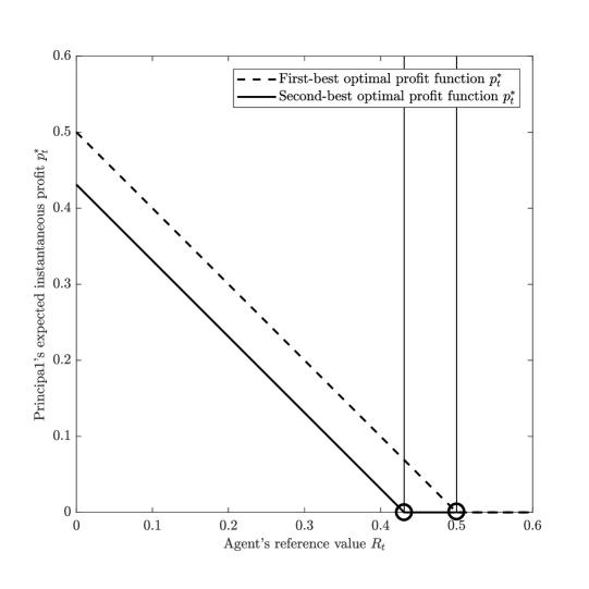
Figure 1: The principal’s expected instantaneous profit functions $p_{t}^{*}$ in the monopsony case with parameters $\sigma=0.2$, $\gamma=4$, $\kappa=0.2$. The dashed curve shows the first-best, the solid curve shows the second-best case. The threshold reference values for each case are illustrated with the circles on the curves and with the vertical dotted lines.

Results in this subsection are equivalent with those obtained from the well-known static Holmström–Milgrom model. Indeed, our dynamic model simply represents a flow of essentially independent one-shot games. However our endogenous treatment for the agent’s participation constraint establishes a connections between different time instances. This leads to non-trivial dynamics for $R_{t}$ that we explore in the next subsection.

3.3 Dynamics of the reference value

In each cases, substituting the optimal contract parameters $a_{t}^{*}$, $s_{t}^{*}$ and $f_{t}^{*}$ into Equation (4), we obtain the dynamics of the reference value $R_{t}$, and in particular, for the perfect competition first-best case as

$$dR_{t}=\begin{cases}-\kappa\,R_{t}\,dt,&R_{t}\geq\frac{1}{2}\\ \kappa\left(\frac{1}{2}-R_{t}\right)dt,&R_{t}<\frac{1}{2}\end{cases}\,,$$ (22)

for the monopsony first-best case as

$$dR_{t}=\begin{cases}-\kappa\,R_{t}\,dt,&R_{t}\geq\frac{1}{2}\\ 0,&R_{t}<\frac{1}{2}\end{cases}\,,$$ (23)

for the perfect competition second-best case as

$$dR_{t}=\begin{cases}-\kappa\,R_{t}\,dt,&R_{t}\geq\frac{1}{2\,\left(1+\gamma\,\sigma^{2}\right)}\\ \kappa\left(\frac{1+2\,\gamma\,\sigma^{2}}{2\,(1+\gamma\,\sigma^{2})^{2}}-R_{t}\right)dt+\kappa\,\frac{\sigma}{1+\gamma\,\sigma^{2}}\,dB_{t},&R_{t}<\frac{1}{2\,\left(1+\gamma\,\sigma^{2}\right)}\end{cases}\,,$$ (24)

and for the monopsony second-best case as

$$dR_{t}=\begin{cases}-\kappa\,R_{t}\,dt,&R_{t}\geq\frac{1}{2\,\left(1+\gamma\,\sigma^{2}\right)}\\ \kappa\,\frac{\gamma\,\sigma^{2}}{2\,(1+\gamma\,\sigma^{2})^{2}}dt+\kappa\,\frac{\sigma}{1+\gamma\,\sigma^{2}}\,dB_{t},&R_{t}<\frac{1}{2\,\left(1+\gamma\,\sigma^{2}\right)}\end{cases}\,.$$ (25)

In both second-best cases, the reference value follows a sticky reflecting Brownian motion on $(-\infty,\bar{r}]$. Starting below $\bar{r}$, the reference value process behaves like a Brownian motion with some drift and variance rate. When the upper boundary $\bar{r}$ is reached, it is reflected back below the boundary. However, the overall time spent at the boundary is positive as the reflection is sticky. See in particular Theorem 5 of Engelbert and Peskir (2014) for the SDE specification of sticky reflecting Brownian motion and the existence of a weak solution.

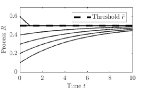
(a) Perfect competition, first-best case

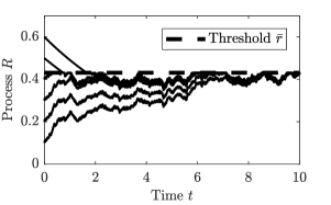
(b) Perfect competition, second-best case

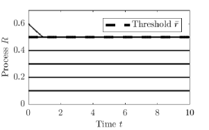
(c) Monopsony, first-best case

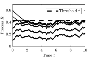
(d) Monopsony, second-best case

Figure 2: Examples of the dynamics of the reference value in the myopic principal setting. The parameters are $\sigma=0.2$, $\gamma=4$, $\kappa=0.2$.

We illustrate the four different dynamics in Figure 2. We show trajectories with different initial reference values. All the trajectories are generated from the simulation of one particular Brownian motion trajectory. In all four cases, if the initial reference value is above the threshold, the players do not contract for a while, and the reference value then decays exponentially. This corresponds to a gig worker who has too high initial demands. He does not find work as the employer cannot realize positive profits by contracting at such high wages. As time passes, out of gig jobs and thus with zero income, the worker’s demands drop. The higher the value of the parameter $\kappa$, the faster the worker is forced to lower his demands, or in other words, the more vulnerable he is.

Below the threshold, the four cases exhibit different dynamics. In the two first-best cases, as there is no random component in the agent’s wage, the dynamics are deterministic (zero volatility in Equations (22)–(23)). In the perfect competition case, the agent absorbs the surplus; therefore, he receives a higher wage than his current reference value. This leads to his reference value increasing and converging to the threshold value. In the monopsony case, the surplus is taken as the principal’s profit, and the agent receives a wage equal to his reference value. This leads to a non-increasing, constant reference value. The second-best dynamics are similar to their respective first-best versions for both the perfect competition and the monopsony cases. However, the threshold values are lower as discussed in the previous subsection, and agent’s reference value becomes stochastic because of the random output share he receives as incentive component of his overall pay.

4 Impact of reference value to the principal’s far-sighted strategies

So far, both the agent and the principal were myopic in the model. In this section, the agent is still myopic, but now we consider a far-sighted principal whose objective is not merely an instantaneous profit, but rather a discounted life-time profit. Perfect competition in our model means that the principal offers a contract that is optimal for the agent, while she is satisfied with zero instantaneous profit. This translates to a zero life-time profit, so there is no room for long-time strategies on the principal’s part. However, a monopsonistic principal is able to realize a positive profit and her aim is to maximize it. In this case, it is meaningful to study far-sighted strategies on the principal’s part. In what follows, we explore whether such far-sighted strategies can increase the principal’s profit and the ways the principal can regulate the agent’s wage demand.

The far-sighted principal’s performance depending on the policies $a_{t}$, $s_{t}$, and $f_{t}$ is measured by the present value of her lifetime profit

$$E_{r}\left[\rho\int_{0}^{\infty}e^{-\rho t}\,(dX_{t}-dW_{t})\right]=E_{r}\left[\rho\int_{0}^{\infty}e^{-\rho t}\,\chi_{t}\,\left((1-s_{t})\,a_{t}-f_{t}\right)dt\right],$$ (26)

where $\rho$ is her subjective discount rate and $E_{r}$ denotes the expectation conditional on $R_{0}=r$. The factor $\rho$ in front of the integrals normalizes total pay-offs to the same scale as flow pay-offs.

Applying a (not necessarily optimal) contract policy $a_{t}$, $s_{t}$, and $f_{t}$, the performance still depends on the agent’s initial reference value $r$. To highlight the significance of the principal’s far-sighted approach, we will calculate the performance for two different policies. First, we explore how the myopic strategy obtained in the previous section performs under the far-sighted objective (Equation (26)). The myopic strategy is, of course, suboptimal, yet it establishes a benchmark for comparison. Next, we will properly solve the control problem defined by Equation (26) and dynamics (4), thereby obtaining the optimal solution. We present our results both for the first-best and for the second-best cases below.

4.1 First-best case

When investigating the suboptimal myopic strategy’s performance under the far-sighted objective, we do not need to solve a new control problem. We simply plug in the optimized myopic control variables $a^{*}_{t}$, $s^{*}_{t}$, $f^{*}_{t}$ from Equations (12)–(14) to Equation (26). We obtain the myopic principal’s suboptimal value function in the first-best case as

$$V^{(sub)}(r) =E_{r}\left[\rho\int_{0}^{\infty}e^{-\rho t}\,\chi_{t}\left(\frac{1}{2}-R_{t}\right)dt\right]\,.$$

If $r\leq\frac{1}{2}$ ($\chi_{0}=1$ in this case), then $dR_{t}=0$ (see Equation (23)), therefore $R_{t}=R_{0}$ and $\chi_{t}=1$ for all times $t$. Without any stochastic effects, the conditional expected value is trivial and we obtain

$$V^{(sub)}(r) =\rho\int_{0}^{\infty}e^{-\rho t}\left(\frac{1}{2}-r\right)dt=\frac{1}{2}-r\,.$$ (27)

If $r>\frac{1}{2}$, then $R_{t}$ decays exponentially to $\bar{r}=\frac{1}{2}$ and then remains constant (see the topmost trajectories in Figure 2(c)). During the decay $\chi_{t}=0$, therefore the instantaneous profit is zero. At the threshold the profit remains zero (cf. Equation (23)), this means that the lifetime profit is also zero. Combining these results we finally obtain

$$V^{(sub)}(r)=\left(\frac{1}{2}-r\right)^{+}\,.$$

Note, this is essentially the same as the profit function obtained for the myopic first-best case (see Equation (15)).

Next, we solve for the optimal first-best value function. As before, the first-best case means that the principal controls not only the $s_{t}$, $f_{t}$ contract variables, but also the agent’s effort $a_{t}$. The first-best optimal value function is thus defined as

$$V(r)=\max_{\{a_{t},s_{t},f_{t}\}_{t\geq 0}}E_{r}\left[\rho\int_{0}^{\infty}e^{-\rho t}\,\chi_{t}\left(\left(1-s_{t}\right)a_{t}-f_{t}\right)dt\right]\,,$$ (28)

where the dynamics of $R_{t}$ is given by Equation (23). We solve the control problem separately for the no-contract and the contract regimes with the help of Hamilton–Jacobi–Bellman (HJB) equations. Details of the solution for this control problem can be found in Appendix A.1. We obtain the optimal contract parameters as

$$a^{*}(r) =1$$ (29)

$$s^{*}(r) =0$$ (30)

$$f^{*}(r) =r+\frac{1}{2},$$ (31)

the threshold as

$$\bar{r} =\frac{\rho}{2\,\left(\kappa+\rho\right)},$$ (32)

and the optimal value function $V$ is continuously differentiable and takes the form

$$V(r)=\begin{cases}\frac{1}{2}-r,&r<\bar{r}\\ \frac{\kappa}{2\,\left(\kappa+\rho\right)}\left(\frac{r}{\bar{r}}\right)^{-\frac{\rho}{\kappa}},&r\geq\bar{r}\end{cases}\,.$$ (33)

We obtain that the myopic and the far-sighted principal implements the same contract (cf. Equations (12)–(14) and Equations (29)–(31)). The required and enforced effort level $a^{*}$ is constant $1$, and the share $s^{*}$ equals zero. The principal does not need to incentivize the agent with a share in the first-best case, only the fix wage $f^{*}$ depends on the reference value $r$. The function $f^{*}(r)$ is the same for both types of principals.

Although there is no difference in the implemented contract parameters for the myopic and the far-sighted principals, the thresholds (see Equations (16) and (32)), and consequently, the value functions (see Equations (27) and (22)) also differ. Figure 3 shows the suboptimal and optimal value functions as the dashed curves. The threshold reference values for each case are illustrated with the circles on the curves and with the vertical dotted lines. We can see that the suboptimal value function is never above the optimal value function (although they coincide in the optimal contract regime), as expected. The threshold is substantially lower for the optimal solution than for the suboptimal. This means there is an interval of reference values, where a principal with the suboptimal myopic strategy would employ the agent (and realize a positive instantaneous profit), but a far-sighted principal would not. The myopic principal is satisfied with the realized positive short-term profit by accommodating the agent’s high wage demand. However, the far-sighted principal takes into account the dynamics of the reference value. She chooses to deny employment, thereby forcing the agent, who is now without gig income, to lower his demand. The contract is only struck after the agent’s reference value drops to a relatively low threshold level, where the principal can realize higher profits. Of course, the temporarily missing production hurts the principal too. However, the principal performs better in the long run, but the produced output decreases. This is a special case of job-rationing. From the principal’s standpoint, the trade-off is between realizing relatively low short-term profits by employing an agent who expects a high wage or to suffer a period of zero profits but then making larger profits employing a less demanding agent.

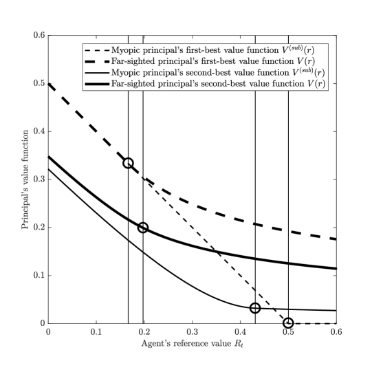
Figure 3: The principal’s value functions in the monopsonistic labor market with parameters $\sigma=0.2$, $\gamma=4$, $\kappa=0.2$, $\rho=0.1$. The threshold reference values for each case are illustrated with the circles on the curves and with the vertical lines.

Inspecting our result for the far-sighted principal’s threshold $\bar{r}$ (Equation (32)) allows for the analysis of this trade-off in terms of the principal’s and agent’s attributes. The value of $\bar{r}$ is indicative of how the principal and the agent share the fruits of production. The higher the threshold is, the higher the wage the agent can secure for himself and the lower the principal’s profit. According to Equation (32), $\bar{r}$ depends on the ratio between $\rho$ and $\kappa$, if $\rho$ is large (small) relative to $\kappa$, $\bar{r}$ becomes larger (smaller). The parameter $\rho$ is the employer’s subjective discount rate, in financial terms her expected return. A large $\rho$ means the employer greatly discounts long-term profits, she is more focused on making profits in the short-term. She cannot afford the delay in production and is forced to employ the worker sooner rather than later, even for a high wage. Her bargaining power is relatively weak and her share of the output will be low. On the other hand, $\kappa$ measures the worker’s vulnerability, the rate at which the worker’s reference value decreases when unemployed (see Equation (4)). The greater $\kappa$, the sooner the worker is ready to take up work, even at low wages. This decreases his bargaining power, his share of the output will be low. Our model thus connects the employer’s and the worker’s relative bargaining power to characteristic time-scale attributes of them. How long can the employer afford to wait for the worker to drop his wage demands? How long can the worker go without contract, and thus without gig income? Whoever can afford to be more patient, will be relatively less vulnerable, and will win out in the wage battle.

So far, we have investigated the principal’s first-best solution. The principal can prescribe and enforce the agent’s effort, thus the effort does not depend on the reference value, it is constant. In this case, there is no need to incentivize the agent with a share of the output. Therefore there is no random component in the wage. The trade-off between incentive and risk-aversion, the risk shift to the worker, inherent in the classical principal-agent literature, has thus been switched off in our analysis. This allowed us to explore the effect of self-respect, and introduce the new, dynamic type of trade-off between the agent’s vulnerability and the principal’s time preference in isolation. In what follows, we turn our attention to the dynamic model’s second-best solution that allows us to explore the interplay between the two types of trade-offs.

4.2 Second-best case

Following the same procedure as in the first-best case, we define the myopic principal’s suboptimal value function in the second-best case as

$$V^{(sub)}(r)=E_{r}\left[\rho\int_{0}^{\infty}e^{-\rho t}\,\chi_{t}\left((1-s^{*}_{t})\,a^{*}_{t}-f^{*}_{t}\right)dt\right]\,,$$ (34)

where now $s^{*}_{t}$, $a^{*}_{t}$, $f^{*}_{t}$ are coming from Equations (17)–(19), threshold $\bar{r}$ from Equation (21), and $R$ follows the dynamics in Equation (25). Details of our calculation can be found in Appendix A.2, here we just present the results. With reference value threshold $\bar{r}=\frac{1}{2\,(1+\gamma\,\sigma^{2}))}$, we obtain

$$V^{(sub)}(r)=\begin{cases}c_{1}\,\exp\{b\,r\}+c_{2}-r,&r<\bar{r}\\ V^{(sub)}(\bar{r})\left(\frac{r}{\bar{r}}\right)^{-\frac{\rho}{\kappa}},&r\geq\bar{r}\end{cases}\,.$$

with parameters

$$V^{(sub)}(\bar{r}) =\frac{1-(\bar{r}-c_{2})\,b}{\frac{\rho}{\kappa}\,\bar{r}^{-1}+b}\,,\quad c_{1}=\frac{1-\frac{\rho}{\kappa}\,V^{(sub)}(\bar{r})\,\bar{r}^{-1}}{b\,\exp\{b\cdot\bar{r}\}}$$

$$c_{2} =\frac{1+\frac{\rho-\kappa}{\rho}\,\gamma\,\sigma^{2}}{2(1+\gamma\,\sigma^{2})^{2}}\,,\quad b=\frac{1}{2\,\kappa}\left(\sqrt{\gamma^{2}+\frac{8\,\rho(1+\gamma\,\sigma^{2})^{2}}{\sigma^{2}}}-\gamma\right)\,.$$

The second-best myopic suboptimal value function we obtain is shown in Figure 3 as the thin solid curve.

Finally, we investigate the optimal control problem for the far-sighted principal in the second-best case. The effort $a_{t}$ is now determined by the agent, guided by the incentive as the principal offers a share of the output and shifts her business risk to the agent. Although now the principal is far-sighted, the agent is still myopic in choosing his effort. Therefore, we obtain the result $a^{*}_{t}=s_{t}$ as in the myopic case (see Equation (18)). The contract variables $s_{t}$ and $f_{t}$ are still at the disposal of the principal, therefore her second-best optimal value function is given as the solution to the control problem

$$V(r)=\max_{\{s_{t},f_{t}\}_{t\geq 0}}E_{r}\left[\rho\int_{0}^{\infty}e^{-\rho t}\,\chi_{t}\left((1-s_{t})\,s_{t}-f_{t}\right)dt\right]\,,$$ (35)

with the dynamics given in Equation (4) and $a_{t}=s_{t}$. A characterization of the solution of this non-trivial control problem is given the following Proposition 1, see Appendix A.3 for the corresponding proof.

Proposition 1.

Consider the optimal control problem in (35) with reference point dynamics given by (4) and $a_{t}=s_{t}$. The corresponding value function ${V}$ is in $C^{2}(\mathbb{R})$ and satisfies the ordinary differential equation

$$0 = \frac{1}{2}\frac{1}{1+\gamma\,\sigma^{2}-\frac{\kappa}{\rho}\,\gamma\,\sigma^{2}\,V^{\prime}(r)-\frac{\kappa^{2}}{\rho}\sigma^{2}\,V^{\prime\prime}(r)}-r-V(r)\,,$$ (36)

on $(-\infty,\bar{r})$, where $\bar{r}$ is a free boundary, with boundary conditions

$$0 = \lim_{r\searrow-\infty}V^{\prime\prime}(r)\,,$$

$$0 = \lim_{r\nearrow\bar{r}}-\kappa\,r\,V^{\prime}(r)-\rho\,V(r)\,,$$

$$0 = \lim_{r\nearrow\bar{r}}-\kappa\,rV^{\prime\prime}(r)-\left[\rho+\kappa\right]\,V^{\prime}(r)\,.$$

On $(\bar{r},\infty)$, the value function satisfies the ordinary differential equation

$$0 = -\kappa\,r\,V^{\prime}(r)-\rho\,V(r)\,,$$

with solution $V(r)=V(\bar{r})\,(r/\bar{r})^{-\rho/\kappa}$, for $r\geq\bar{r}$, and $V(\bar{r})=\lim_{r\nearrow\bar{r}}V(r)$. The corresponding optimal control is given by

$${a}^{*}_{t} = {s}^{*}_{t}\,,$$

$${f}^{*}_{t} = {\bf 1}_{R_{t}<\bar{r}}\,\left(R_{t}-\left({s}^{*}_{t}\right)^{2}/2+\gamma\,\sigma^{2}\,\left({s}^{*}_{t}\right)^{2}/2\right)\,,$$

$${s}^{*}_{t} = {\bf 1}_{R_{t}<\bar{r}}\,\frac{1}{1+\gamma\,\sigma^{2}-\frac{\kappa}{\rho}\,\gamma\,\sigma^{2}\,V^{\prime}(R_{t})-\frac{\kappa^{2}}{\rho}\sigma^{2}\,V^{\prime\prime}(R_{t})}\,.$$

Note that these results still contain differential equations that need to be solved. The second order differential equation for $V$ on $(-\infty,\bar{r})$ in (36) is non-linear and a well-known path to a closed-form solution does not exits. Thus, we solve the differential equations numerically. In particular, we employ a Picard-type iteration and some heuristics motivated by our results of the previous cases to determine the free boundary $\bar{r}$. In all our numerical calculation the scheme works well and produces a candidate that indeed satisfies the differential equations characterizing the unique smooth solution. See Appendix A.4 for details.

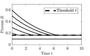
(a) Monopsony, first-best case

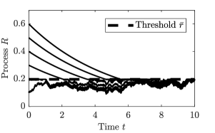
(b) Monopsony, second-best case

Figure 4: Examples of the dynamics of the reference value with optimal strategies in the far-sighted principal setting. The parameters are $\sigma=0.2$, $\gamma=4$, $\kappa=0.2$, $\rho=0.1$.

The second-best optimal value function we obtain is shown in Figure 3 as the thick solid curve. We can see that the second-best optimal value function is strictly lower than the first-best. This is but natural, as in the case of the first-best solution the principal has a higher degree of control in the form of directly enforcing the agent’s effort. However, a new feature in the second-best case is that the optimal value function (thick solid curve) is strictly higher than the suboptimal (thin solid curve) even in the contract regime. This is different from the behavior of the first-best curves (thick and thin dashed curves) and can be explained by the different types of reference value dynamics, see Figure 4. In the first-best case, the dynamics is deterministic. In fact, in the contract regime the reference value stays constant. This means that in the contract regime, the optimal and suboptimal strategies are equivalent, resulting in equal value functions for the principal. This is different in the second-best case, where the principal always offers a share from the output leading to stochastic dynamics in the contract regime. Accordingly, the suboptimal strategy indeed comes into effect for all possible reference values in both the contract and no-contract regime.

5 Effort policy, output, profit and wage levels

In this section, we explore implications of our model variants on the implemented effort levels, on the produced output, and on the agent’s and principal’s benefits. To this end, we define and calculate the instantaneous expected output $x_{t}$, the agent’s instantaneous expected wage $w_{t}$, and his instantaneous expected net wage $\tilde{w}_{t}$ in an analogous manner to the principal’s instantaneous expected profit $p_{t}$ (see Equation (1)). To ease up the language, in what follows, we will often omit the instantaneous and the expected classifiers for these quantities. All results will be presented assuming the more interesting monopsonistic labor market.

5.1 Reference value dependence

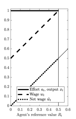
(a) Myopic principal, first-best case

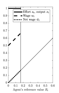
(b) Far-sighted principal, first-best case

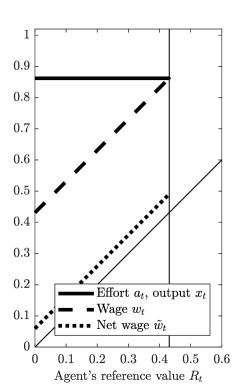
(c) Myopic principal, second-best case

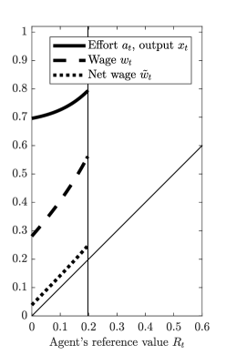
(d) Far-sighted principal, second-best case

Figure 5: The agent’s effort $a_{t}$ (expected output $x_{t}$), expected wage $w_{t}$, and expected net wage $\tilde{w}_{t}$ in the monopsonistic labor market. The parameters are $\sigma=0.2$, $\gamma=4$, $\kappa=0.2$, $\rho=0.1$.

In this subsection, we show the quantities of interest implied by our model, as functions of the agent’s reference value. As the reference value is a running average of the agent’s realized net wages, these curves can also be thought of as representing path-dependence in the model. The four panels in Figure 5 give a comparison along the myopic versus far-sighted, and along the first-best versus second-best dimensions. In all our model variants, the instantaneous expected output $x_{t}$ always equals to the agent’s effort level $a^{*}$, therefore these are both shown as the solid curves. The dashed curves, and the dotted curves show the wage, and the net wage, respectively. The gap between the output and the wage curves represents the principal’s profit, while the gap between the wage and the net wage is the cost of effort. The threshold reference value is shown as a vertical upper limit for the plotted functions’ domain. For easy comparison between the forward-looking net wage, and the backward-looking averaged net wage (which is the reference value itself), we also plotted the identity function as a thin solid line on each panel.

Comparing the top two panels (Figure 5(a), 5(b)) we see that the only difference between the myopic first-best and the far-sighted first-best solutions is in the threshold reference value. In accordance with our earlier discussions, for the myopic principal the threshold is simply set by her non-negative profit condition. The far-sighted principal however enforces a lower wage level for the agent, thereby securing a positive profit for herself even at the (much lower) threshold. As in the first-best cases the reference value is stationary, the net wage curves align with the identity curves.

When considering the second-best solution, the principal needs to offer a share of the output to incentivize the agent. Our model in this case yields for the contract share $s^{*}=a^{*}=x_{t}$, therefore in the bottom panels the solid curves also represent the share functions. The non-zero share implies uncertainty in the wage of the risk-averse agent, which has several consequences. The contracted effort, the produced output, and the expected wage all shift lower in the second-best panels (Figure 5(c), 5(d)) compared to their first-best counterparts (Figure 5(a), 5(b)). We interpret these diminishing values being due to costs of the incentives the principal needs to offer. On the other hand, the net wages are now higher than the reference values (see the identity lines and the dotted curves above them in Figures 5(c) and 5(d)). This means the forward-looking expected net wage is greater than the backward-looking average of realized net wages. The difference is the cost of the wage uncertainty, for which the principal must compensate the agent.

Comparing the effort policies in the second-best cases, we observe that the principal implements lower effort levels and a lower threshold in the far-sighted case, compared to the myopic case. Both of these differences indicate the far-sighted principal’s ability to regulate future wage expectation of the agent by setting the expected output and hence the expected net wage lower. On the far-sighted, second-best panel (Figure 5(d)), unlike on all the others, the output and wage curves exhibit convexity. This is stemming from the fact that this is the only case, when the reference value dynamics is stochastic, the principal can control its volatility, and she cares about the reference value’s distance from the threshold. We offer an intuition to explain the convexity of the share function. Closer to the threshold reference value, the principal benefits from increasing the wage volatility, which she can achieve by raising the share contract parameter. Whatever happens next, it is advantageous for her. If the reference moves down, the agent’s future wage demand will be lower. If the reference moves upwards, it means both the output and her profit will be high, and if the reference hits the threshold, she will not offer work anyway. The increasing effort policy in the far-sighted second-best case implies that the share parameter and the induced effort level are path-dependent.

5.2 Vulnerability and self-exploitation of the worker

Here, we examine how the worker’s vulnerability parameter $\kappa$ affects the produced output, the worker’s effort and his wage level. We calculate the quantities of interest at the $\bar{r}$ threshold, as we focus on the best possible situation for the worker in our analysis. The results presented in this subsection involve a monopsonic labor market, and a far-sighted principal. First, we show results with the agent’s vulnerability parameter confined on a scale similar to the principal’s discount parameter ($\rho=0.1$ and $\kappa\in[0,0.3]$). In the first-best case we can give analytic expressions for the quantities of the interest. As $\bar{r}=\frac{\rho}{2(\kappa+\rho)}$ (see Equation (32)), we obtain

$$x_{t} =a_{t}=1,$$

$$w_{t} =\bar{r}+\frac{1}{2}=\frac{2\,\rho+\kappa}{2\,(\rho+\kappa)}$$

$$\tilde{w}_{t} =\bar{r}=\frac{\rho}{2\,(\kappa+\rho)}$$

for the output, wage and net wage. In the second-best case, we cannot obtain analytical formulas for these quantities, so we use the numerical method mentioned above to determine them.

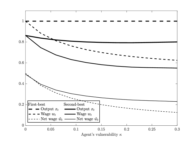
Figure 6: Effects of the agent’s vulnerability parameter $\kappa$ on the output $x_{t}$, wage $w_{t}$ and net wage $\tilde{w}_{t}$ for $R_{t}=\bar{r}$. The labor market is monopsonistic, the principal is far-sighted and the parameters are $\sigma=0.2$, $\gamma=4$, $\kappa=0.2$, $\rho=0.1$. The agent’s vulnerability parameter $\kappa$ is of the same order of magnitude as the principal’s discount parameter $\rho$. Output $x_{t}$ is equal to the agent’s effort $a_{t}$, and in the second-best case, is also equal to the share $s_{t}$.

In Figure 6, dashed curves show our results for the first-best case, and the second-best results are shown as solid curves. The top thick curves represent the output $x_{t}$. They also represent the agent’s effort $a_{t}$, and the solid top thick curve also represents $s_{t}$ in the second-best case (see Equation (8)). The middle curves show the agent’s wage. This is the gross wage that is actually handed to the worker. The bottom thin curves represent the net wage; these are lower than their respective middle counterparts because the cost of effort is subtracted from the gross wage. In other words, the gap between the middle and bottom thin curves represent the agent’s cost of effort.

In the first-best case, the principal has direct control over the agent’s effort; therefore she enforces a constant, high effort level ($a_{t}=1$). This leads to a constant high-level output ($x_{t}=1$) as well. As the agent’s vulnerability parameter $\kappa$ grows, his gross wage and his net wage both decrease with a constant cost of effort gap between them. Vulnerability is reflected in the fact that by increasing $\kappa$, the agent works the same amount, but earns less and less.

The second-best case is more complicated. The principal does not have direct control over the effort; therefore she needs to incentivize the agent. This leads to a high share value $s_{t}$, which introduces uncertainty in the risk-averse agent’s wage. Because this incentivization vs. risk-aversion trade-off is made, the agent’s effort and thus the output becomes smaller compared to the first-best case. The gross wage becomes smaller, while the net wage becomes higher, with a smaller cost of effort gap between them. Although the agent’s earning is now smaller, but he also has to work less, and therefore his net wage, interpreted as his utility, becomes higher. Both of these quantities still decrease with the growing vulnerability of the agent, but their decay is less pronounced compared to the first-best case. These differences that all favor the agent one way or another can all be explained with the principal’s reduced level of control.

Now consider the situation when the worker is extremely vulnerable. Figure 7 shows the same quantities as Figure 6, but now the vulnerability parameter $\kappa$ can be an order of magnitude higher than the employer’s discount parameter $\rho$. The dashed curves representing the first-best case do not show new phenomena. The output (and the worker’s effort) is constant, and the worker’s wage and net wage still steadily decrease.

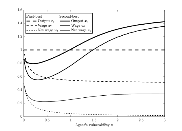
Figure 7: Effects of the agent’s vulnerability parameter $\kappa$ on the output $x_{t}$, wage $w_{t}$ and net wage $\tilde{w}_{t}$ for $R_{t}=\bar{r}$. The labor market is monopsonistic, the principal is far-sighted and the parameters are $\sigma=0.2$, $\gamma=4$, $\kappa=0.2$, $\rho=0.1$. The agent’s vulnerability parameter $\kappa$ is an order of magnitude larger than the principal’s discount parameter $\rho$. Output $x_{t}$ is equal to the agent’s effort $a_{t}$, and in the second-best case, is also equal to the share $s_{t}$.

The second-best case is more interesting (see the solid curves in Figure 7). After the declining phase discussed above (see Figure 6), the output, the wage, and the net wage all tend to increase. Above a certain $\kappa$, the effect of incentivization and so the risk shift to the worker becomes very pronounced as the employer offers more and more share of the output. In fact, the share becomes even greater than one, which means that the employer not only offers all the output to the worker but also complements it with an output-proportional premium. As the incentive increases, the worker chooses to invest more and more effort and thus the output and his gross wage also increases. On the other hand, the worker’s net wage only increases moderately and soon levels off. The relative weakness of the worker in this regime is exhibited in a new way: as his vulnerability increases, he works harder and harder, but his net wage (essentially, his utility) remains nearly constant. This phenomenon represents self-exploitation in our model.

6 Conclusion

In the new world of gig works, where collective action is less and less effectual against the risk shift, individual strategies become more and more important. We introduced a dynamic principal-agent model that captures the psychological and financial challenges facing the worker due to the risk shift, which is the essential determinant of the gig economy. Our model’s central idea is self-respect as a coping mechanism for the worker. His self-respect-driven behavior – based on the worker’s lived experience –, represents an individual heuristic strategy that puts the worker in a better bargaining position even in unfavorable labor market situations. This strategy may occasionally lead to discontinuation of work, as the employer does not meet the worker’s seemingly exaggerated wage demand. This lull in production hurts the employer as well, which is the source of the worker’s bargaining power.

In the gig economy, the rapidly changing environment demands flexibility from the participants, but all too often this happens to the detriment of the worker. His wage demand which is based on his lived experience ensures a sort of income stability for him in face of ever-changing job conditions. The extent to which the worker can employ this heuristic strategy is characterized by a vulnerability parameter in our model. A vulnerable worker will receive lower wages for the same job, and in extreme cases we see self-exploitation – he works more and more for a marginally higher income and is forced to bear extremely high personal risks.

There are many possibilities for further research. We observed that the principal implements lower and increasing effort levels and a lower threshold in the far-sighted case, compared to the myopic case. The implied path dependence could explain patterns observed in the gig economy. It is possible to extend our model with unemployment benefits and calculate the average amount of time the agent spends unemployed at the ergodic distribution over his reference value. We conjecture that unemployment benefits in such a setting could increase employment, as opposed to decreasing it, as predicted by neoclassical models. One can also adjust the building blocks of our framework to a specific application of contingent work to gain more insights. For example, our framework relates to the managerial power theory in executive compensation from the 2000s, see Bebchuk and Fried (2003). The mostly verbally formulated theory broadly states that the agent-manager can impose his compensation demands on the firm-principal. We can formalize this relationship in our setup as follows: the agent-manager forms his compensation demands by his past experience as given by our reference value and the ability to impose his demands is captured by our vulnerability parameter. Thus, our framework provides a basis for putting the managerial power theory in a formal model allowing theoretical predictions and subsequent empirical analyses.

Appendix A Appendix

For the model specified in section 2, we now impose conditions on the agent’s and principal’s strategy, $a$ and $(s,f)$, respectively, to guarantee the existence of the related stochastic process. Our model is Markovian with effective state process $R$, and therefore we focus on feedback strategies. The agent’s effort level is a stochastic process $a=\{a_{t},0\leq t<\infty\}$ given by a non-negative bounded function of $R$, that is, $a_{t}=a(R_{t})$ for some measurable function $a$ such that $0\leq a(r)\leq C_{a}$, for all $r\in\mathbb{R}$ and some $C_{a}>0$. The share is a stochastic process $s=\{s_{t},0\leq t<\infty\}$ given by a bounded function of $R$, that is, $s_{t}=s(R_{t})$ for some measurable function $s$ such that $|s(r)|\leq C_{s}$, for all $r\in\mathbb{R}$ and some $C_{s}>0$. The fixed component is a stochastic processes $f=\{f_{t},0\leq t<\infty\}$ given by a function of $R$, that is, $f_{t}=f(R_{t})$ for some measurable function $f$ such that $|f(r)|\leq c_{f}+C_{f}|r|$, for all $r\in\mathbb{R}$ and some $c_{f},C_{f}>0$.

A.1 Far-sighted principal: First-best optimal

The formulation of the problem as well as from the results in section 3 suggest that no contract is struck above a threshold $\bar{r}$, that is to be determined.

The HJB equation corresponding to value function $V$ in Equation (28) with dynamics of $R$ in Equation (4) is

$$\rho V(r)=-\kappa rV^{\prime}(r),$$

for the no-contract regime, $r\geq\bar{r}$, and

$$\rho V(r)=\max\limits_{\{a,s,f\}}\left\{\rho\left((1-s)a-f\right)+\kappa(s\,a+f-\frac{1}{2}a^{2}-r)V^{\prime}(r)+\frac{1}{2}\kappa^{2}\sigma^{2}s^{2}V^{\prime\prime}(r)\right\}$$

for the contract regime, $r<\bar{r}$. In the no-contract regime, we obtain

$$V(r) =V(\bar{r})\left(\frac{r}{\bar{r}}\right)^{-\frac{\rho}{\kappa}},\text{ for }r\geq\bar{r}.$$

In the contract regime, $r<\bar{r}$, the term in the HJB depending on $f$ and that has to be maximized is of the form

$$-\rho f+\kappa fV^{\prime}(r).$$

As the value function is non-increasing, that is, $V^{\prime}(r)\leq 0$, the optimal $f$ is the minimal choice such that a contract is struck ($u_{t}\geq R_{t}$). In other words

$$f^{*} =r-sa+\frac{a^{2}}{2}+\frac{s^{2}}{2}\gamma\sigma^{2}\,,$$

see also Equation (10). For $r<\bar{r}$, we can thus write down the reduced HJB equation only in terms of $a$ and $s$ as control variables

$$\rho V(r)=\max_{\{a,s\}}\left\{\rho\left(a-\frac{1}{2}a^{2}-\frac{1}{2}\gamma\sigma^{2}s^{2}-r\right)+\frac{1}{2}\kappa\gamma\sigma^{2}s^{2}V^{\prime}(r)+\frac{1}{2}\kappa^{2}\sigma^{2}s^{2}V^{\prime\prime}(r)\right\}.$$

Optimizing with respect to $a$ first, and then optimizing with respect to $s$ using that $V$ is convex, that is, $V^{\prime\prime}(r)\geq 0$, we obtain the optimal controls as

$$a^{*} =1$$

$$s^{*} =0,$$

and by back-substitution, we obtain an equation for the value function

$$V(r) =\frac{1}{2}-r,\text{ for }r<\bar{r}.$$

We still have to determine the threshold $\bar{r}$ and $V(\bar{r})$ to completely characterize the solution. The latter follows from the continuity of $V$ what is a direct consequence of its specification in (28), leading to

$$V(\bar{r}) =\frac{1}{2}-\bar{r}.$$

For any given threshold $\bar{r}$, the value function as specified so far satisfies the HJB. Denote by $r^{\prime}$ an arbitrary threshold and define

$$V(r;r^{\prime}) =\left\{\begin{array}[]{ll}\frac{1}{2}-r,&\hbox{ for }r<r^{\prime}\\ \left(\frac{1}{2}-r^{\prime}\right)(r/r^{\prime})^{-\frac{\rho}{\kappa}},&\hbox{ for }r\geq r^{\prime}.\end{array}\right.$$

The optimality condition pinning down $\bar{r}$ is obtained as the first order condition in $r^{\prime}$ on the relevant region $r\geq r^{\prime}$, that is

$$0 =\partial_{r^{\prime}}V(r;\bar{r})=-(r/\bar{r})^{-\frac{\rho}{\kappa}}+\frac{\rho}{\kappa}\left(\frac{1}{2}-\bar{r}\right)(r/\bar{r})^{-\frac{\rho}{\kappa}}\,\bar{r}^{-1}$$

with solution

$$\bar{r} =\frac{\rho}{2(\kappa+\rho)}.$$

From there, it follows that $\lim_{r\searrow\bar{r}}V^{\prime}(r)=-1=\lim_{r\nearrow\bar{r}}V^{\prime}(r)$, that is, the value function $V$ is continuously differentiable.

A.2 Far-sighted principal: Second-best suboptimal

In the no-contract regime, that is, for $r\geq\bar{r}$, with $\bar{r}=1/(2(1+\gamma\sigma^{2}))$ given in Equation (21), the differential equation describing the value function and the form of its solution are still the same as in previous cases

$$\rho V^{(sub)}(r) =-\kappa r{V^{(sub)}}^{\prime}(r),\text{ for }r>\bar{r}$$

$$V^{(sub)}(r) =V^{(sub)}(\bar{r})\left(\frac{r}{\bar{r}}\right)^{-\frac{\rho}{\kappa}}\,\text{ for }r\geq\bar{r}.$$

In contrast to the previous case, the threshold $\bar{r}$ is a priori, but as before, the value $V^{(sub)}(\bar{r})$ is still to be determined.

In the contract regime, that is, for $r<\bar{r}$, the effort $a^{*}$, the share $s^{*}$ and the fix wage $f^{*}$ are determined by the myopic strategy (see Equations (17)–(19)). The Feynman Kac formula applied to (34) gives

$$\rho V^{(sub)}(r)=\rho\left(\frac{1}{2}s^{*}-r\right)+\frac{1}{2}\kappa\gamma\sigma^{2}s^{*2}{V^{(sub)}}^{\prime}(r)+\frac{1}{2}\kappa^{2}\sigma^{2}s^{*2}{V^{(sub)}}^{\prime\prime}(r),$$ (37)

which is a second order linear ODE. We look for the solution in the form

$$V^{(sub)}(r)=-r+c_{1}\cdot\exp\{b\cdot r\}+c_{2},$$

where $c_{1}$, $c_{2}\in\mathbb{R}$ and $b>0$ are constants. The strict inequality $b>0$ results from the boundary condition $\lim_{r\searrow-\infty}V^{(sub)}(r)=c_{2}-r$, for some constant $c_{2}$. The derivatives of the function $V^{(sub)}(r)$ take the form

$${V^{(sub)}}^{\prime}(r) =-1+c_{1}\cdot b\cdot\exp\{b\cdot r\},$$

$${V^{(sub)}}^{\prime\prime}(r) =c_{1}\cdot b^{2}\cdot\exp\{b\cdot r\}.$$

Substituting these to the Equation (37), we obtain

$$c_{1}\exp\{b\cdot r\}\left(1-\frac{1}{2\rho}\kappa\gamma\sigma^{2}{s^{*}}^{2}\cdot b-\frac{1}{2\rho}\kappa^{2}\sigma^{2}{s^{*}}^{2}\cdot b^{2}\right)-\frac{1}{2}s^{*}+\frac{1}{2\rho}\kappa\gamma\sigma^{2}{s^{*}}^{2}+c_{2}=0.$$ (38)

The expression in the parentheses is the coefficient of the exponential part while the rest is a constant. For Equation (38) to hold for all $r$, both components must individually be zero. From these we obtain

$$c_{2}=\frac{1+\frac{\rho-\kappa}{\rho}\gamma\sigma^{2}}{2(1+\gamma\sigma^{2})^{2}}$$

and the positive solution to the quadratic

$$b=\frac{1}{2\kappa}\left(\sqrt{\gamma^{2}+\frac{8\rho(1+\gamma\sigma^{2})^{2}}{\sigma^{2}}}-\gamma\right).$$

This leaves us with $V^{(sub)}(\bar{r})$ and $c_{1}$ to be determined.

By its definition in (34) we see that $V^{(sub)}$ is continuously differentiable. Using the continuity in $\bar{r}$ ($\lim_{r\nearrow\bar{r}}V^{(sub)}(r)=\lim_{r\searrow\bar{r}}V^{(sub)}(r)$)

$$-\bar{r}+c_{1}\exp\{b\cdot\bar{r}\}+c_{2}=V^{(sub)}(\bar{r}),$$

and the smoothness in $\bar{r}$ ($\lim_{r\nearrow\bar{r}}{V^{(sub)}}^{\prime}(r)=\lim_{r\searrow\bar{r}}{V^{(sub)}}^{\prime}(r)$)

$$-1+c_{1}\cdot b\cdot\exp\{b\cdot\bar{r}\}=-\frac{\rho}{\kappa}V^{(sub)}(\bar{r})\bar{r}^{-1}$$

we obtain

$$V^{(sub)}(\bar{r})=\frac{1-(\bar{r}-c_{2})b}{\frac{\rho}{\kappa}\bar{r}^{-1}+b}$$

and

$$c_{1}=\frac{1-\frac{\rho}{\kappa}V^{(sub)}(\bar{r})\bar{r}^{-1}}{b\exp\{b\cdot\bar{r}\}}.$$

A.3 Far-sighted principal: Second-best optimal

Proof of Proposition 1.

The HJB equation corresponding to the optimal control problem in Equation (35) reads

$$0 = \max_{\{s,f\}}\left\{-\kappa\,r\,V^{\prime}+\chi\left(\kappa\left[f+\frac{s^{2}}{2}\right]V^{\prime}+\frac{\kappa^{2}\sigma^{2}s^{2}}{2}V^{\prime\prime}+\rho\left[s-s^{2}-f\right]\right)\right\}-\rho\,V\,.$$

We maximize the expression that becomes active when $\chi=1$ , that is, on the set $D=\{(r,f,s):f+s^{2}/2-\gamma\,\sigma^{2}\,s^{2}/2\geq r\}$ we analyze

$$G(r;f,s,V^{\prime},V^{\prime\prime}) = \kappa\left[f+\frac{s^{2}}{2}\right]V^{\prime}+\frac{\kappa^{2}\sigma^{2}s^{2}}{2}V^{\prime\prime}+\rho\left[s-s^{2}-f\right]\,.$$

The function $G$ is linear in the fixed salary rate $f$ with coefficient $\kappa\,V^{\prime}-\rho$. By the structure of the payoff we see that $v$ is nonincreasing in $r$, that is, $V^{\prime}\leq 0$, and thus we obtain directly that $\kappa\,V^{\prime}-\rho\leq-\rho<0$. Accordingly, the optimal choice is taking the minimal possible value for $f$ satisfying the constraint given by the set $D$, that is,

$$f^{*}(r;s,V^{\prime},V^{\prime\prime})=r-s^{2}/2+\gamma\,\sigma^{2}\,s^{2}/2\,.$$

Plug $f^{*}(r;s)$ in $G$ and write in abuse of notation

$$G(r;s,V^{\prime},V^{\prime\prime}) = \kappa\left[r+\gamma\,\sigma^{2}\,s^{2}/2\right]V^{\prime}+\frac{\kappa^{2}\sigma^{2}s^{2}}{2}V^{\prime\prime}+\rho\left[s-r-s^{2}/2-\gamma\,\sigma^{2}\,s^{2}/2\right]\,.$$

The first order condition is

$$\partial_{s}G(r;s,V^{\prime},V^{\prime\prime}) = \kappa\,\gamma\,\sigma^{2}\,s\,V^{\prime}+\kappa^{2}\sigma^{2}\,s\,V^{\prime\prime}+\rho\left[1-s-\gamma\,\sigma^{2}\,s\right]\,.$$

To obtain the optimal share $s^{*}$ the sign of the squared term $s^{2}$ in $G$ is important.
Case (a): For $\kappa\,\gamma\,\sigma^{2}\,V^{\prime}+\kappa^{2}\sigma^{2}\,V^{\prime\prime}-\rho-\rho\,\gamma\,\sigma^{2}<0$, the optimal choice for $s$ is given by

$$s^{*}(r,V^{\prime},V^{\prime\prime}) = \frac{1}{1+\gamma\,\sigma^{2}-\frac{\kappa}{\rho}\,\gamma\,\sigma^{2}\,V^{\prime}-\frac{\kappa^{2}}{\rho}\sigma^{2}\,V^{\prime\prime}}\,.$$ (39)

Case (b): Now, consider $\kappa\,\gamma\,\sigma^{2}\,V^{\prime}+\kappa^{2}\sigma^{2}\,V^{\prime\prime}-\rho-\rho\,\gamma\,\sigma^{2}\geq 0$. This implies the optimal policy $|s^{*}|=\infty$. As $f^{*}$ and $a^{*}$ are already determined, both depending on $s$, the state process $R$ has the following dynamics

$${\rm d}R_{t} = \frac{1}{2}\,\kappa\,\gamma\,\sigma^{2}\,s_{t}^{2}\,{\rm d}t+\kappa\,\sigma\,s_{t}\,{\rm d}B_{t}.$$

For $|s_{t}|\nearrow\infty$, the process $R$ is immediately pushed upwards until a lower boundary, say, $\underline{r}$, is reached. At $\underline{r}$ we have $\kappa\,\gamma\,\sigma^{2}\,V^{\prime}+\kappa^{2}\sigma^{2}\,V^{\prime\prime}-\rho-\rho\,\gamma\,\sigma^{2}=0$. However, a boundary $\underline{r}$ is a contradiction to the lower linear bound of $V$ given by $V^{(sub)}$. Thus, we can conclude that the optimal choice for $s^{*}$ is given in (39).
For $\chi=1$, the HJB simplifies to

$$0 = \frac{\rho}{2}s^{*}(r,V^{\prime},V^{\prime\prime})-\rho\,r-\rho\,V\,,$$

or,

$$0 = \frac{1}{2}\frac{1}{1+\gamma\,\sigma^{2}-\frac{\kappa}{\rho}\,\gamma\,\sigma^{2}\,V^{\prime}-\frac{\kappa^{2}}{\rho}\sigma^{2}\,V^{\prime\prime}}-r-V\,.$$

Next, consider the case $\chi=0$ and the HJB reads

$$0 = -\kappa\,r\,V^{\prime}-\rho\,V\,.$$

The principal optimally chooses between the regime $\chi=1$ where an acceptable contract is offered to the agent and the regime where no acceptable contract is offered, that is, $\chi=0$. The HJB results in

$$0 = \max\left\{\frac{1}{2}\frac{\rho}{1+\gamma\,\sigma^{2}-\frac{\kappa}{\rho}\,\gamma\,\sigma^{2}\,V^{\prime}-\frac{\kappa^{2}}{\rho}\sigma^{2}\,V^{\prime\prime}}-\rho\,r;-\kappa\,r\,V^{\prime}\right\}-\rho\,V\,.$$

This is a variational inequality formulation. Denote by $\bar{r}$ the threshold separating the two regimes, that is

$$\bar{r}=\inf\left\{r\in\mathbb{R}:\frac{1}{2}\frac{\rho}{1+\gamma\,\sigma^{2}-\frac{\kappa}{\rho}\,\gamma\,\sigma^{2}\,V^{\prime}(r)-\frac{\kappa^{2}}{\rho}\sigma^{2}\,V^{\prime\prime}(r)}-\rho\,r=-\kappa\,r\,V^{\prime}(r)\right\}\,.$$

Focusing on the regime where the principal offers the agent an acceptable contract $(-\infty,\bar{r})$, then

$$0 = \frac{1}{2}\frac{\rho}{1+\gamma\,\sigma^{2}-\frac{\kappa}{\rho}\,\gamma\,\sigma^{2}\,V^{\prime}(r)-\frac{\kappa^{2}}{\rho}\sigma^{2}\,V^{\prime\prime}(r)}-\rho\,r-\rho\,V(r)\,,\text{ for }r<\bar{r}$$

$$0 = \lim_{r\nearrow\bar{r}}-\kappa\,r\,V^{\prime}(r)-\rho\,V(r)\,,$$

$$0 = \lim_{r\searrow-\infty}V^{\prime\prime}(r)\,.$$

The first boundary condition in the second line is a direct consequence of the variational inequality formulation of the HJB. The second boundary condition in the third line results from linear upper bound (first-best case) and lower bound (suboptimal second-best case). The upper boundary $\bar{r}$ is a free boundary and we need an additional boundary condition to pin down its location. Applying the optimality of $\bar{r}$, the first-order derivative boundary condition can be differentiated to obtain the needed additional boundary condition; it is sometimes called super contact condition, see Sec. 4.6 in Dixit [1993] for a related situation. In the following, this condition is derived.

At $\bar{r}$ the state process is reflected. The reflection is costly in economic terms, see Dixit [1993]. For $R=\bar{r}$, we have that

$${\rm d}R = -\kappa\,\bar{r}\,{\rm d}t\,,\text{ and }\chi=0\,.$$

The value at the non contract point $\bar{r}$ is given by the value of the discounted future income stream when the state process drifts in the region where the agent is offered an acceptable contract. Noting that ${\rm d}R$ is negative write

$$V(\bar{r}+{\rm d}R) = {E}\left[e^{-\rho\,{\rm d}t}\,V(\bar{r})\right]\,\,\,=\,\,\,V(\bar{r})-\rho\,V(\bar{r})\,{\rm d}t\,,$$

and

$$0 = \left(-\kappa\,\bar{r}\,\frac{V(\bar{r}+{\rm d}R)-V(\bar{r})}{{\rm d}R}-\rho\,V(\bar{r})\right)\,{\rm d}t\,,$$

giving

$$0 = \lim_{r\nearrow\bar{r}}-\kappa\,r\,V^{\prime}(r)-\rho\,V(r)\,.$$

This boundary condition holds for any exogenously specified barrier $r^{\prime}$ separating contract and no contract region, that is, for $\chi_{t}={\bf 1}_{R_{t}<r^{\prime}}$. Denote by $V(\cdot;r^{\prime})$ the solution to the original problem with this constraint, that is, a potentially suboptimal choice of offering a contract that is accepted whenever $R<r^{\prime}$, that is, $\chi_{t}={\bf 1}_{R_{t}<r^{\prime}}$. Then $V(\cdot;r^{\prime})$ is characterized on $(-\infty,r^{\prime})$ by

$$0 = \frac{1}{2}\frac{\rho}{1+\gamma\,\sigma^{2}-\frac{\kappa}{\rho}\,\gamma\,\sigma^{2}\,V^{\prime}(r;r^{\prime})-\frac{\kappa^{2}}{\rho}\sigma^{2}\,V^{\prime\prime}(r;r^{\prime})}-\rho\,r-\rho\,V(r;r^{\prime})\,,\text{ for }r<r^{\prime}$$

$$0 = \lim_{r\nearrow r^{\prime}}-\kappa\,r\,V^{\prime}(r;r^{\prime})-\rho\,V(r;r^{\prime})\,,$$

$$0 = \lim_{r\searrow-\infty}V^{\prime\prime}(r;r^{\prime})\,,$$

with notation $V^{\prime}(r;r^{\prime})=\partial_{r}V(r;r^{\prime})$ and $V^{\prime\prime}(r;r^{\prime})=\partial_{rr}V(r;r^{\prime})$. The function $V(\cdot;r^{\prime})$ is extended to $(r^{\prime},\infty)$ by

$$0 = -\kappa\,r\,V^{\prime}(r;r^{\prime})-\rho\,V(r;r^{\prime})\,,\text{ for }r>r^{\prime},$$

or $V(r;r^{\prime})=V(r^{\prime};r^{\prime})\,(r/r^{\prime})^{-\rho/\kappa}$, for $r>r^{\prime}$. The optimality of $\bar{r}$ given by

$$0 = \partial_{r^{\prime}}V(r;\bar{r})\,,\text{ for }r\in\mathbb{R}\,.$$

Differentiating the latter in the variable $r$ gives

$$0 = \partial_{r\,r^{\prime}}V(r;\bar{r})\,\,\,=\,\,\,\partial_{r^{\prime}}V^{\prime}(r;\bar{r})\,,\text{ for }r\in\mathbb{R}\,,$$

where we assumed enough regularity to interchange the order of differentiation. Next, we specify the function $W$ by

$$W(r^{\prime}) = -\kappa\,r^{\prime}\,V^{\prime}(r^{\prime}-;r^{\prime})-\rho\,V(r^{\prime}-;r^{\prime})\,,\text{ for }r^{\prime}\in\mathbb{R}\,,$$

which is zero by the boundary condition at $r^{\prime}$, and compute its derivative

$$0\,\,\,=\,\,\,\partial_{r^{\prime}}W(r^{\prime}) = -\kappa\,V^{\prime}(r^{\prime}-;r^{\prime})-\kappa\,r^{\prime}\left(V^{\prime\prime}(r^{\prime}-;r^{\prime})+\partial_{r^{\prime}}V^{\prime}(r^{\prime}-;r^{\prime})\right)$$

$$-\rho\,\left(V^{\prime}(r^{\prime}-;r^{\prime})+\partial_{r^{\prime}}V(r^{\prime}-;r^{\prime})\right)\,.$$

At $\bar{r}$ we apply the optimality condition and its differentiated version, that is, $0=\partial_{r^{\prime}}V(r;\bar{r})$ and $0=\partial_{r^{\prime}}V^{\prime}(r;\bar{r})$, to see

$$0 = -\kappa\,\bar{r}V^{\prime\prime}(\bar{r}-;\bar{r})-\left[\rho+\kappa\right]\,V^{\prime}(\bar{r}-;\bar{r})\,.$$

One can also check that first and second derivative of $V(\cdot;\bar{r})$ are continuous at $\bar{r}$. Therefore, $V\in C^{2}(\mathbb{R})$. ∎

A.4 Far-sighted principal: Second-best optimal (numerical solution technique)

In the no-contract regime, the HJB equation for the value function is still the same as in previous cases

$$\rho V_{0}(r)=-\kappa rV_{0}^{\prime}(r).$$ (40)

In the contract regime, the optimal fix wage $f^{*}$ is determined as before (see Equation (10)). We can thus write down the reduced HJB equation only in terms of $s$ as a control variable

$$\rho V_{1}(r)=\max_{s}\left\{\rho\left(s-\frac{s^{2}}{2}\left(1+\gamma\sigma^{2}\right)-r\right)+\frac{1}{2}\kappa\gamma\sigma^{2}s^{2}V_{1}^{\prime}(r)+\frac{1}{2}\kappa^{2}\sigma^{2}s^{2}V_{1}^{\prime\prime}(r)\right\}.$$ (41)

Optimizing with respect to $s$, we obtain the optimal control as

$$s^{*}(r)=\frac{\rho}{\rho\left(1+\gamma\sigma^{2}\right)-\gamma\kappa\sigma^{2}V_{1}^{\prime}(r)-\kappa^{2}\sigma^{2}V_{1}^{\prime\prime}(r)},$$ (42)

and by back-substitution, we obtain a differential equation for the value function

$$V_{1}(r)=\frac{1}{2}\cdot\frac{\rho}{\rho\left(1+\gamma\sigma^{2}\right)-\gamma\kappa\sigma^{2}V_{1}^{\prime}(r)-\kappa^{2}\sigma^{2}V_{1}^{\prime\prime}(r)}-r.$$ (43)

Comparing Equation (42) and (43) we can write down a simple relation between the value function and the optimal share function:

$$V_{1}(r)=\frac{1}{2}\cdot s^{*}(r)-r.$$ (44)

Equation (43) is a second-order non-linear ODE with one particular solution

$$\hat{V}_{1}(r)=\frac{1}{2}\cdot\frac{\rho}{\rho\left(1+\gamma\sigma^{2}\right)+\gamma\kappa\sigma^{2}}-r.$$ (45)

Although we have analytical particular solution, we cannot solve the ODE in its most general form.

We use an implicit iterative method on a fine discrete grid for the reference value $r$. We start with a reasonable initial value function $V$ that spans both the contract and no-contract regimes. In the no-contract regime, we use the implicit discrete approximation

$$V_{0}^{\prime}(r)=\frac{V_{0}(r)-V(r-\Delta r)}{\Delta r}.$$ (46)

In the contract regime, we use the implicit discrete approximations

$$V_{1}^{\prime}(r) =\frac{V(r+\Delta r)-V(r-\Delta r)}{2\Delta r}$$ (47)

$$V_{1}^{\prime\prime}(r) =\frac{V(r+\Delta r)+V(r-\Delta r)-2V_{1}(r)}{(\Delta r)^{2}}.$$ (48)

Plugging Equation (46) into Equation (40) we obtain

$$V_{0}(r)=\frac{\kappa r}{\kappa r+\rho\Delta r}V(r-\Delta r).$$

Using Equation (44) we determine function $s(r)$ from $V(r)$. This is a good approximation if the iteration is close to converging. This also means we use Equation (41) without the maximization with respect to $s$, we simply assume that the $s(r)$ calculated from $V(r)$ is close to the optimal $s^{*}(r)$ function. Plugging (47) and (48) into (41) (without $s$ maximization), we obtain

$$V_{1}(r)=\frac{1}{\rho(\Delta r)^{2}+\kappa^{2}\sigma^{2}s^{2}(r)}\Bigg{[}\rho(\Delta r)^{2}\left(s(r)-\frac{s^{2}(r)}{2}\left(1+\gamma\sigma^{2}\right)-r\right)+\\ +\frac{1}{2}\gamma\kappa\sigma^{2}s^{2}(r)(\Delta r)\left(V\left(r+\Delta r\right)-V\left(r-\Delta r\right)\right)+\frac{1}{2}\kappa^{2}\sigma^{2}s^{2}(r)\left(V(r+\Delta r)+V(r-\Delta r)\right)\Bigg{]}.$$

Next we calculate the updated value function as

$$V^{(new)}(r)=\max\left\{V_{0}(r),V_{1}(r)\right\}.$$

We repeat this iteration until $V^{(new)}(r)$ is sufficiently close to $V(r)$.

For small $r$ values we use the boundary condition derived from Equation (45), for large $r$ values we assume zero curvature at the boundary.

References

- Abel [1990] Abel, A. B. 1990. Asset prices under habit formation and catching up with the Joneses. The American Economic Review 80(2):38–42. https://www.jstor.org/stable/2006539.
- Allon, Cohen, and Sinchaisri [2018] Allon, G., M. Cohen, and W. P. Sinchaisri. 2018. The impact of behavioral and economic drivers on gig economy workers. Available at SSRN 3274628 https://dx.doi.org/10.2139/ssrn.3274628.
- Ashford, Caza, and Reid [2018] Ashford, S. J., B. B. Caza, and E. M. Reid. 2018. From surviving to thriving in the gig economy: A research agenda for individuals in the new world of work. Research in Organizational Behavior 38:23–41. https://doi.org/10.1016/j.riob.2018.11.001.
- Battigalli and Dufwenberg [2009] Battigalli, P., and M. Dufwenberg. 2009. Dynamic psychological games. Journal of Economic Theory 144(1):1–35. https://doi.org/10.1016/j.jet.2008.01.004.
- Bebchuk and Fried [2003] Bebchuk, L. A., and J. M. Fried. 2003. Executive compensation as an agency problem. Journal of Economic Perspectives 17(3):71–92. https://doi.org/10.1257/089533003769204362.
- Bester [1989] Bester, H. 1989. Incentive-compatible long-term contracts and job rationing. Journal of Labor Economics 7(2):238–55. https://doi.org/10.1086/298207.
- Bieber and Moggia [2021] Bieber, F., and J. Moggia. 2021. Risk shifts in the gig economy: The normative case for an insurance scheme against the effects of precarious work. Journal of Political Philosophy 29(3):281–304. https://doi.org/10.1111/jopp.12233.
- Bolton and Dewatripont [2005] Bolton, P., and M. Dewatripont. 2005. Contract theory. Cambridge, Massachusetts, USA: The MIT Press. ISBN 978-0-262-02576-8.
- Broughton et al. [2018] Broughton, A., R. Gloster, R. Marvell, M. Green, J. Langley, and A. Martin. 2018. The experiences of individuals in the gig economy. Department for Business, Energy and Industrial Strategy. https://www.gov.uk/government/publications/gig-economy-research.
- Carreño and Faus [2021] Carreño, B., and J. Faus. 2021. Spain’s gig economy poses labour rights conundrum as regulation eyed. Reuters. March 3. https://reut.rs/3S3W8xl. Retrieved: 28 March 2021.
- Cave [1983] Cave, G. 1983. Job rationing, unemployment, and discouraged workers. Journal of Labor Economics 1(3):286–307. https://doi.org/10.1086/298014.
- Conger [2020] Conger, K. 2020. Uber and Lyft drivers in California will remain contractors. The New York Times. Nov 4. https://nyti.ms/3b4WX8p. Retrieved: 28 March 2021.
- Cvitanić and Zhang [2012] Cvitanić, J., and J. Zhang. 2012. Contract theory in continuous-time models. Springer Science & Business Media. ISBN 978-3-642-14199-7. 10.1007/978-3-642-14200-0.
- DellaVigna et al. [2017] DellaVigna, S., A. Lindner, B. Reizer, and J. F. Schmieder. 2017. Reference-dependent job search: Evidence from Hungary. The Quarterly Journal of Economics 132(4):1969–2018. https://doi.org/10.1093/qje/qjx015.
- DeMarzo and Sannikov [2006] DeMarzo, P. M., and Y. Sannikov. 2006. Optimal security design and dynamic capital structure in a continuous-time agency model. The Journal of Finance 61(6):2681–724. https://doi.org/10.1111/j.1540-6261.2006.01002.x.
- Dixit [1993] Dixit, A. K. 1993. The art of smooth pasting, vol. 55. Chur, Switzerland: Harwood Academic Publisher. ISBN 3-7186-5384-2.
- Dube et al. [2020] Dube, A., J. Jacobs, S. Naidu, and S. Suri. 2020. Monopsony in online labor markets. American Economic Review: Insights 2(1):33–46. https://doi.org/10.1257/aeri.20180150.
- Eliaz and Spiegler [2018] Eliaz, K., and R. Spiegler. 2018. Managing intrinsic motivation in a long-run relationship. Economics Letters 165:6–9. https://doi.org/10.1016/j.econlet.2018.01.018.
- Engelbert and Peskir [2014] Engelbert, H.-J., and G. Peskir. 2014. Stochastic differential equations for sticky Brownian motion. Stochastics An International Journal of Probability and Stochastic Processes 86(6):993–1021. https://doi.org/10.1080/17442508.2014.899600.
- Geanakoplos, Pearce, and Stacchetti [1989] Geanakoplos, J., D. Pearce, and E. Stacchetti. 1989. Psychological games and sequential rationality. Games and Economic Behavior 1(1):60–79. https://doi.org/10.1016/0899-8256(89)90005-5.
- Harrison and Lemoine [1981] Harrison, J. M., and A. J. Lemoine. 1981. Sticky Brownian motion as the limit of storage processes. Journal of Applied Probability 18(1):216–26. https://doi.org/10.2307/3213181.
- Holmström and Milgrom [1987] Holmström, B., and P. Milgrom. 1987. Aggregation and linearity in the provision of intertemporal incentives. Econometrica: Journal of the Econometric Society 303–28. https://doi.org/10.2307/1913238.
- Jacobs, Kolb, and Taylor [2017] Jacobs, J. A., A. M. Kolb, and C. R. Taylor. 2017. Optimal reputation systems for platforms. Working Paper, Duke University. https://faculty.fuqua.duke.edu/ioconference/papers/2017/2%20Aaron%20Kolb__JKTplatforms.pdf.
- Jacobs, Kolb, and Taylor [2018] ———. 2018. Communities, co-ops, and clubs: Social capital and incentives in large collective organizations. Working Paper, Kelley School of Business Research Paper. https://dx.doi.org/10.2139/ssrn.3155391.
- Kerényi [2021] Kerényi, P. 2021. Incentives in the gig economy. ECONOMY AND FINANCE: ENGLISH-LANGUAGE EDITION OF GAZDASÁG ÉS PÉNZÜGY 8(2):146–63. https://doi.org/10.33908/EF.2021.2.2.
- Kőszegi and Rabin [2006] Kőszegi, B., and M. Rabin. 2006. A model of reference-dependent preferences. The Quarterly Journal of Economics 121(4):1133–65. https://doi.org/10.1093/qje/121.4.1133.
- Lundesgaard [2001] Lundesgaard, J. 2001. The Holmström–Milgrom model: A simplified and illustrated version. Scandinavian Journal of Management 17(3):287–303. https://doi.org/10.1016/S0956-5221(99)00039-1.
- Macera [2018a] Macera, R. 2018a. Intertemporal incentives under loss aversion. Journal of Economic Theory 178:551–94. https://doi.org/10.1016/j.jet.2018.10.003.
- Macera [2018b] ———. 2018b. Present or future incentives? On the optimality of fixed wages with moral hazard. Journal of Economic Behavior & Organization 147:129–44. https://doi.org/10.1016/j.jebo.2017.12.004.
- Mortensen [1986] Mortensen, D. T. 1986. Job search and labor market analysis. In O. Ashenfelter and D. Card, eds., Handbook of Labor Economics, vol. 2, chap. 15, 849–919. Elsevier. https://doi.org/10.1016/S1573-4463(86)02005-9.
- Piskorski and Westerfield [2016] Piskorski, T., and M. M. Westerfield. 2016. Optimal dynamic contracts with moral hazard and costly monitoring. Journal of Economic Theory 166:242–81. https://doi.org/10.1016/j.jet.2016.08.003.
- Pollak [1970] Pollak, R. A. 1970. Habit formation and dynamic demand functions. Journal of Political Economy 78(4, Part 1):745–63. https://doi.org/10.1086/259667.
- Rawls [1971] Rawls, J. 1971. A theory of justice. The Belknap Press of Harvard University Press, Cambridge, Massachusetts. ISBN 0-674-01772-2.
- Reuters [2020] Reuters. 2020. Spain’s supreme court rules food delivery riders are employees, not freelancers. Reuters. September 23. https://reut.rs/3Oykf4g. Retrieved: 28 March 2021.
- Rogerson [1985] Rogerson, W. P. 1985. Repeated moral hazard. Econometrica: Journal of the Econometric Society 69–76. https://doi.org/10.2307/1911724.
- Sannikov [2008] Sannikov, Y. 2008. A continuous-time version of the principal-agent problem. The Review of Economic Studies 75(3):957–84. https://doi.org/10.1111/j.1467-937X.2008.00486.x.
- Santibáñez, Possamaï, and Zhou [2020] Santibáñez, N. H., D. Possamaï, and C. Zhou. 2020. Bank monitoring incentives under moral hazard and adverse selection. Journal of Optimization Theory and Applications 184(3):988–1035. https://doi.org/10.1007/s10957-019-01621-9.
- Spreitzer, Cameron, and Garrett [2017] Spreitzer, G. M., L. Cameron, and L. Garrett. 2017. Alternative work arrangements: Two images of the new world of work. Annual Review of Organizational Psychology and Organizational Behavior 4:473–99. https://doi.org/10.1146/annurev-orgpsych-032516-113332.
- Stewart and Stanford [2017] Stewart, A., and J. Stanford. 2017. Regulating work in the gig economy: What are the options? The Economic and Labour Relations Review 28(3):420–37. https://doi.org/10.1177%2F1035304617722461.
- Van den Berg [1990] Van den Berg, G. J. 1990. Nonstationarity in job search theory. The Review of Economic Studies 57(2):255–77. https://doi.org/10.2307/2297381.
- Wang and Yang [2019] Wang, C., and Y. Yang. 2019. Optimal self-enforcement and termination. Journal of Economic Dynamics and Control 101:161–86. https://doi.org/10.1016/j.jedc.2018.12.010.
- Wood [2018] Wood, A. J. 2018. Powerful times: Flexible discipline and schedule gifts at work. Work, Employment and Society 32(6):1061–77. https://doi.org/10.1177%2F0950017017719839.
- Woodcock [2020] Woodcock, J. 2020. The algorithmic panopticon at Deliveroo: Measurement, precarity, and the illusion of control. Ephemera: Theory & Politics in Organization 20(3). http://www.ephemerajournal.org/sites/default/files/pdfs/contribution/20-3Woodcock.pdf.
- Wu et al. [2019] Wu, Q., H. Zhang, Z. Li, and K. Liu. 2019. Labor control in the gig economy: Evidence from Uber in China. Journal of Industrial Relations 61(4):574–96. https://doi.org/10.1177%2F0022185619854472.
- Zhu [2012] Zhu, J. Y. 2012. Optimal contracts with shirking. The Review of Economic Studies 80(2):812–39. https://doi.org/10.1093/restud/rds038.