Flux and storage of energy in non-equilibrium, stationary states

Abstract

Systems kept out of equilibrium in stationary states by an external source of energy store an energy $\Delta U=U-U_{0}$. $U_{0}$ is the internal energy at equilibrium state, obtained after the shutdown of energy input. We determine $\Delta U$ for two model systems: ideal gas and Lennard-Jones fluid. $\Delta U$ depends not only on the total energy flux, $J_{U}$, but also on the mode of energy transfer into the system. We use three different modes of energy transfer where: the energy flux per unit volume is (i) constant; (ii) proportional to the local temperature (iii) proportional to the local density. We show that $\Delta U/J_{U}=\tau$ is minimized in the stationary states formed in these systems, irrespective of the mode of energy transfer. $\tau$ is the characteristic time scale of energy outflow from the system immediately after the shutdown of energy flux. We prove that $\tau$ is minimized in stable states of the Rayleigh-Benard cell.

Systems out of equilibrium are notoriously difficult to describe in a single coherent methodology based on variational principles. Principles such as Prigogine minimum entropy production jaynes1980 , Attard second entropy variation attard2008 or, Ziegler maximum entropy production martyushev2013 etc. suggested over the last 100 years, have not reached the same status as the maximum entropy principle known from equilibrium thermodynamics vita2010 ; bartlett2016 ; velasco2011 . A new paradigm, such as the driven lattice gas system, is believed to become an "Ising model" for non-equilibrium statistical physics katz1984 ; zia2010 ; stinchcombe2001 ; pleimling2010 ; dickman2018 ; zia2002 . Steady State Thermodynamics (SST) is yet another description framework for non-equilibrium stationary states, which is still being developed dickman2014 ; pradhan2011 ; sasa2006 ; oono1998 . Here we present a different approach to stationary states, based on two quantities: the energy stored in non-equilibriums states, $\Delta U$, and the total energy flux, $J_{U}$ in these states.

The second law of thermodynamics states that the entropy of a system has its maximum value at the equilibrium state. Entropy, $S$, is a function of state, thus for an isolated system of $N$ molecules of total internal energy $U$ enclosed in a volume, $V$ , the entropy has a fixed value $S=S(U,V,N)$. Internal constraints make it possible to divide the system into $n$ isolated subsystems of entropies $S_{i}=S(U_{i},V_{i},N_{i})$ for $i=1\cdots n$ , where $\sum_{i}^{n}N_{i}=N$, $\sum_{i}^{n}V_{i}=V$, $\sum_{i}^{n}U_{i}=U$. The maximum entropy principle states callen1985 ; holyst2012 that $S(U,V,N)\geq\sum_{i}^{n}S_{i}$. We develop a similar methodology for non-equilibrium stationary states, by introducing internal constraints in these states. Next we make a conjecture on variational principles for these states. We do not claim the generality of this conjecture, but simply prove it for three studied cases. In order to illustrate our methodology we study two systems: ideal gas and Lennard-Jones fluid. Next we test our methodology on two competing states in the Rayleigh-Benard (RB) cell cross1993 . Summarizing our results obtained for these systems: we find that $\Delta U$ is minimized in non-equilibrium stationary states for a fixed $J_{U}$. Minimization is with respect to all constrained states of the system, similarly as in equilibrium thermodynamics. Due to the lack of a general theoretical framework for describing the non-equilibrium systems under consideration, we are not able to formulate a general argument for the validity of the conjectured principle. Nevertheless, it is plausible that, under well defined conditions, the energy storage obeys some sort of variational principle. In the search for this principle we employed dimensional analysis and considered the relevant physical quantities. This analysis suggests the ratio $\Delta U/J_{U}$, which has the dimension of time and a nice physical interpretation, as a candidate for the quantity to be extremized.

Ideal gas between two planar walls: An ideal gas is confined between two planar walls of surface area $\mathcal{A}$ located at $z=\pm L$. The temperature of the walls is constant $T_{-L}=T_{L}=T_{0}$. Energy is supplied to the volume of the fluid (e.g. by microwaves). In stationary states the total flux of energy into the system, $J_{U}$, matches the total flux at the walls. In the hydrodynamic limit, the time evolution of the system is given by the conservation laws for mass, momentum, and energy supplemented by the relations between thermodynamic forces and fluxes and thermodynamic equations of state. For an ideal gas $U=(3/2)Nk_{B}T$, $p=\rho k_{B}T$, where $U$ is the internal energy, $p$ is the pressure, $\rho=N/V$ is the number density of a fluid, $V$ is the volume, $N$ is the number of gas particles and $k_{B}$ is the Boltzmann constant. We observed in our previous simulations/calculations babin2005 ; holyst2008 for gas-liquid evaporating systems that mechanical equilibrium is established very fast (in comparison to heat flow). Therefore we also expect a constant pressure across the system in this case. The stationary state satisfies $\mathbf{v}=0$ (gas velocity), $p=const$ babin2005 ; holyst2008 . These two equations come from the conservation of mass and momentum. (The same results, i.e., $\mathbf{v}=0$ and $p=const$ in the stationary states are also obtained in MD simulations of the Lennard-Jones system described later.) The conservation of energy is given by $\nabla\cdot\mathbf{j}_{\varepsilon}(\mathbf{r})=\sigma_{\varepsilon}$, where $\mathbf{j}_{\varepsilon}(\mathbf{r})$ is local heat flux and $\sigma_{\varepsilon}$ is the external heat source. The integral of $\sigma_{\varepsilon}$ over the volume is $\int_{V}\sigma_{\varepsilon}=J_{U}$. The local flux of energy per unit area is proportional to the temperature gradient $\mathbf{j}_{\varepsilon}=-\kappa\nabla T$, where $\kappa$ is the thermal conductivity and thus:

$$-\kappa\nabla^{2}T(\mathbf{r})=\sigma_{\varepsilon}.$$ (1)

We solve Eq(1) for three forms of the source term describing different manners of energy supply: (i) $\sigma_{\varepsilon}=\lambda_{1}$, (ii) $\sigma_{\varepsilon}=\lambda_{2}T(z)$, and (iii) $\sigma_{\varepsilon}=\lambda_{3}\rho(z)$. The equations are transformed into dimensionless form by rescaling the variables $\tilde{z}=z/L$, $\tilde{T}=T/T_{0}$ and $\tilde{\rho}=\rho/\rho_{0}$ together with (i) $\tilde{\lambda}_{1}=\lambda_{1}L^{2}/(\kappa T_{0})$, (ii) $\tilde{\lambda}_{2}=\lambda_{2}L^{2}/\kappa$, and (iii) $\tilde{\lambda}_{3}=\lambda_{3}L^{2}\rho_{0}/(\kappa T_{0})$, with $\lambda_{i}>0,i=1,2,3$. Here, $\rho_{0}$ is the number density of the ideal gas at temperature $T_{0}$ and pressure $p_{0}$. The temperature is a function of coordinate $z$, only. In all these cases we introduce energy directly into the volume. This mode of energy transfer is well known by e.g. electromagnetic waves (microwaves , visible light etc.). If we couple a microwave device with a thermovision camera we can in principle add energy to hotter places (where density is low) or to less hot spots, where density is high. Thus the three modes of energy transfer are physically feasible.

For case (i) the equation for stationary temperature profile is $d^{2}\tilde{T}(\tilde{z})/d\tilde{z}^{2}=-\tilde{\lambda}_{1}$ with symmetric boundary conditions $\tilde{T}(-1)=\tilde{T}(1)=1$. This equation has the solution $\tilde{T}(\tilde{z})=-\frac{\tilde{\lambda}_{1}}{2}(\tilde{z}^{2}-1)+1$. The energy of this stationary state is calculated using the assumption of local equilibrium. The energy density field $U/(V\rho_{0}T_{0})=\varepsilon(\tilde{T}(\tilde{z}),\tilde{\rho}(\tilde{z}))=(3/2)k_{B}\tilde{\rho}(\tilde{z})\tilde{T}(\tilde{z})$ for an ideal gas. Upon rescaling by the equilibrium value $U_{0}/(V\rho_{0}T_{0})=\varepsilon_{0}=(3/2)k_{B}$, the dimensionless local energy density $\tilde{\varepsilon}=\varepsilon/\varepsilon_{0}$ obeys $\tilde{\varepsilon}(\tilde{T}(\tilde{z}),\tilde{\rho}(\tilde{z}))/\tilde{T}(\tilde{z})=\tilde{\rho}(\tilde{z})$. Our system does not exchange molecules with the environment therefore the number of particles is constant. This condition is given by the equation $\int_{-1}^{1}\tilde{\rho}(\tilde{z})d\tilde{z}=2$ and thus implies $\int_{-1}^{1}d\tilde{z}\tilde{\varepsilon}(\tilde{T}(\tilde{z}),\tilde{\rho}(\tilde{z}))/\tilde{T}(\tilde{z})=2$. The reduced pressure obeys $\tilde{p}=\tilde{T}(\tilde{z})\tilde{\rho}(\tilde{z})=\tilde{\varepsilon}(\tilde{T}(\tilde{z}),\tilde{\rho}(\tilde{z}))$, thus since $\tilde{p}$ is constant, so is $\tilde{\varepsilon}$. We obtain $\tilde{\varepsilon}$ as

$$\tilde{\varepsilon}=\frac{2}{\int_{-1}^{1}d\tilde{z}/\tilde{T}(\tilde{z})}.$$ (2)

Integrating the temperature profile we obtain

$$\tilde{\varepsilon}(\tilde{\lambda}_{1})=\frac{\sqrt{\tilde{\lambda}_{1}(\tilde{\lambda}_{1}+2)}}{2\mathrm{tanh}^{-1}\Bigg{(}\sqrt{\frac{\tilde{\lambda}_{1}}{\tilde{\lambda}_{1}+2}}\Bigg{)}}.$$ (3)

For cases (ii) and (iii) of the external flux see Supplemental Material (SM).

We introduce a rigid, impenetrable, adiabatic wall in the system at $z=z_{1}$. The wall divides the system into two subsystems (1) and (2). The internal energy at equilibrium is $U_{0}=2L\mathcal{A}\varepsilon_{0}$, the same as in the unconstrained system. We calculate the storage of energy over its equilibrium value, $\Delta U_{1}+\Delta U_{2}=U_{1}+U_{2}-U_{0}$ in the same way as presented above. The division into two subsystems satisfies the following conditions in our methodology: 1) The subsystems are in mutual equilibrium after the shutdown of energy input, so that no additional fluxes appear after removal of the constraints at equilibrium. 2) The subsystems reach a stationary state characterized by $U_{1}$, $U_{2}$ and fluxes $J_{U_{1}}$, $J_{U_{2}}$. 3) The mode of energy transfer to each subsystem is the same. Since $J_{U}=\mathcal{A}\int_{-L}^{L}\sigma_{\varepsilon}dz$ we obtain for case (i):

$$\frac{\Delta U}{J_{U}}=\frac{\varepsilon_{0}}{\lambda_{1}}\Big{(}\tilde{\varepsilon}-1\Big{)}$$ (4)

and

$$\frac{\Delta U_{1}+\Delta U_{2}-U_{0}}{J_{U_{1}}+J_{U_{2}}}=\frac{\varepsilon_{0}}{\lambda_{1}}\Big{(}f_{1}(\tilde{z}_{1})+f_{2}(\tilde{z}_{1})-1\Big{)}$$ (5)

with

$$f_{1}(\tilde{z}_{1})=\frac{(1-\tilde{z}_{1})\sqrt{\Lambda^{(1)}_{-}(\Lambda^{(1)}_{-}+2)}}{4\mathrm{tanh}^{-1}\Big{(}\sqrt{\frac{\Lambda^{(1)}_{-}}{\Lambda^{(1)}_{-}+2}}\Big{)}}\qquad\mathrm{and}\qquad f_{2}(\tilde{z}_{1})=\frac{(1+\tilde{z}_{1})\sqrt{\Lambda^{(1)}_{+}(\Lambda^{(1)}_{+}+2)}}{4\mathrm{tanh}^{-1}\Big{(}\sqrt{\frac{\Lambda^{(1)}_{+}}{\Lambda^{(1)}_{+}+2}}\Big{)}}$$ (6)

where $\tilde{z}_{1}=L_{1}/L$, $\Lambda^{(1)}_{-}=\tilde{\lambda}_{1}(1-\tilde{z}_{1})^{2}$ and $\Lambda^{(1)}_{+}=\tilde{\lambda}_{1}(1+\tilde{z}_{1})^{2}$. By inspection, in the range $0\leq\tilde{z}_{1}<1$ the functions $f_{i}(\tilde{z}_{1}),i=1,2$ are positive and lie above their tangent lines at $\tilde{z}_{1}=0$, i.e., $f_{i}(\tilde{z}_{1})>f^{\prime}_{i}(\tilde{z}_{1})\big{|}_{\tilde{z}_{1}=0}\tilde{z}_{1}+\frac{\varepsilon}{2},\;i=1,2$ for fixed $\tilde{\lambda}_{1}>0$. Since $f_{1}(\tilde{z}_{1})=f_{2}(-\tilde{z}_{1})$ one has $f^{\prime}_{1}(\tilde{z}_{1})\big{|}_{\tilde{z}_{1}=0}=-f^{\prime}_{2}(\tilde{z}_{1})\big{|}_{\tilde{z}_{1}=0}$ and hence $f_{1}(\tilde{z}_{1})+f_{2}(\tilde{z}_{1})>2\frac{\varepsilon}{2}$ which proves that

$$\frac{\Delta U_{1}+\Delta U_{2}}{J_{U_{1}}+J_{U_{2}}}\geq\frac{\Delta U}{J_{U}}.$$ (7)

The equality holds only for equal partition of the system into two subsystems ($z_{1}=0$). This equation states that the energy stored in two subsystems is larger than in the unconstrained system for a fixed flux $J_{U}=J_{U_{1}}+J_{U_{2}}$. This observation holds irrespective of the sign of $\Delta U$ i.e. irrespective of the equilibrium reference state footnote . Cases (ii) and (iii) also satisfy Eq. (7) (discussed in SM). Additionally in SM we present calculations of case (i) with $\kappa={\rm const}\sqrt{T}$ (expected for the dilute gas), which further confirm Eq. (7) for this system. It is well understood that a true ideal gas would have non-interacting particles with a zero collision cross section. We use the equation of state of the ideal gas as an approximation for the interacting gas characterized by finite, temperature dependent, $\kappa$.

Lennard-Jones liquid in a rectangular box: In order to perform analytical calculations for the ideal gas model we had to assume local equilibrium. This assumption is inherent in irreversible thermodynamics equations. In order to test our analytical results for the ideal gas model we performed Molecular Dynamics (MD) simulations of Lennard-Jones system. MD simulations provided qualitatively the same results as analytical calculations presented in the previous section. In the MD simulations Newton equations of motion are solved, thus no assumptions concerning local equilibirum or constancy of heat conductivity are made. Nevertheless, during MD simulations our system stays quite close to local equilibrium. In general we can expect a violation of the local equilibrium assumption only when the flux of the energy flowing across the system is faster than the process of local distribution of energy between all degrees of freedom. Such conditions are expected in e.g. shock waves.

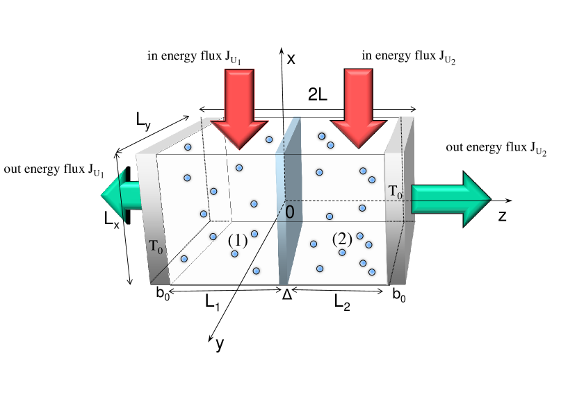
Figure 1: Lennard-Jones simulation box with the shaded region in the middle dividing the system into (1) and (2) subsystems of size $L_{1}$ and $L_{2}$ respectively. The finite size of this wall precludes interactions between the molecules in different subsystems. Heating is indicated by the red arrows. Cooling is performed at the boundaries at a distance $b_{0}$ from two walls and shown schematically by the green arrows. The fluxes $J_{U_{1}}$ and $J_{U_{2}}$ in and out are equal in the stationary state. The total size of the system $L$ is fixed.

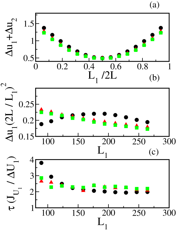
Figure 2: (a) Energy stored $\Delta u_{1}+\Delta u_{2}$ per LJ atom in subsystem (1) and (2) as a function of the size of one subsystem $L_{1}$ for a fixed flux $J_{U}=J_{U_{1}}+J_{U_{2}}$. The flux of energy per unit volume is constant (red triagles); proportional to temperature (black circles); proportional to density(green squares). The minimal value of $\Delta U_{1}+\Delta U_{2}=\Delta U$ is equal to the value for the unconstrained system for $L_{1}=L_{2}$ (see Eq(7)). (b) The energy (per particle) in subsystem (1) as a function of $L_{1}$. This energy scales as $U_{1}/V\sim L_{1}^{2}$. It is not an extensive quantity, since the energy at equilibrium $U_{0}/V\sim{const}$. (c) The characteristic time $\tau$ of energy out-flow from the sub-system (1) after the shutdown of energy flux into the sub-system. Energy decreases as $\exp(-t/\tau)$ (see SM) with an initial decay time $\tau=2\Delta U_{1}/J_{U_{1}}$. Factor 2 appears because the out-flow of energy is only by one wall.

In all the simulations we set the flux constant for the system and subsystems i.e. $J_{U}=J_{U_{1}}+J_{U_{2}}$. We also set the same $J_{U}$ for all the modes of energy transfer into the system. Thus we make a comparison between different cases using only one parameter, i.e., the energy $\Delta U$ stored in a system. Molecular Dynamics (MD) simulations allen1987 ; verlet1967 (Fig.1) were performed in the system of fixed number $N=266240$ of Lennard-Jones (LJ) atoms. The simulation box was divided into two subsystems (1) and (2) of sizes $L_{1}$ and $L_{2}$, respectively. The total size $L_{1}+L_{2}$ of the box was constant. Energy was added only to the regions (1),(2) (Fig.1) once per 10 time steps in three manners (i),(ii),(iii) as described for the ideal gas model. When the flux of energy was proportional to the density each LJ atom received the same amount of kinetic energy. For flux proportional to temperature the portion of energy added to each atom was proportional to its kinetic energy. For energy flux proportional to volume the same amount of energy was added to the same volume, i.e., all the atoms in a given volume received a given amount of energy equally shared between them. All temperature and density profiles in the stationary states are shown in SM for the system with and without internal walls. In Fig. 2a we show the dependence of the energy $\Delta U$ stored in the system, as a function of the size $L_{1}$ of one subsystem for fixed fluxes $J_{U}=J_{U_{1}}+J_{U_{2}}$. This figure contains results for all three scenarios of the energy transfer. All physical quantities are given in LJ units. When $L_{1}=L_{2}$, $\Delta U$ reaches a minimal value (equal to the value obtained for the unconstrained system) as expected from Eq(7). In Fig(2b) we show the scaling of the energy per particle stored in the subsystem (1) as a function of the size of the subsystem $L_{1}$. Finally we observe that after the shutdown of energy flux into the system, the energy decreases as $\exp(-t/\tau)$ (see SM) at short times, with a decay time $\tau=\Delta U/J_{U}$ (Fig(2c)). In summary, the MD simulations of LJ fluid confirm Eq. (7). In most of our simulations the system was in a single phase state, but we also confirmed Eq. (7) for the two-phase non-equilibrium system. We observed a spontaneous phase separation and the two phases present in the stationary state with a liquid at the cold boundary and a heated gas inside the simulation box. In these simulations we could not obtain stationary states with convection (as in the Rayleigh-Benard cell) irrespective of the value of the energy flux input into the system.

2D Rayleigh Benard system of hard discs (HD): We further tested Eq. (7) in the Rayleigh-Benard (RB) cell (Fig(3) for two competing stationary states. One is called the conductive state Fig(3b) and second one the convective state as shown in Fig(3c). For small temperature gradients the conductive state is stable, while for large temperature gradients it is the convective state that is stable. We use the internal walls to stabilize the conductive state above the transition to the convective state. This methodology allows for comparison of $\Delta U/J_{U}$ for both states at the same gravitational field and temperatures at the walls.

Discs of diameter $\sigma$ and mass $m$, were placed in a rectangular simulation box of size $L_{x}d\times L_{y}d$ (where $d=\sigma/\sqrt{0.4}$). Two sizes were studied $50d\times 100d$ (the small system) and $100d\times 100d$ (the large system). The dimensionless density, $\rho^{*}=N\sigma^{2}/(L_{x}L_{y}d^{2})=0.4$. The upper plate had a constant temperature $T_{0}$, the lower plate was heated to temperatures $T=T^{*}\times T_{0}$, with $T^{*}\geq 1$. All the disks were subjected to a gravitational force ${F}=m(0,-g)$. The HD fluid was simulated with event-driven dynamics, where discs followed parabolic trajectories between collisions.The discs collided in an elastic manner with the side walls and between themselves. The collisions with the upper and lower plates allowed for a transfer the thermal energy to the system. Upon collision with the upper or lower plate the disc velocity was drawn from the Maxwell distribution corresponding to the temperature of the plate and the direction was chosen randomly from $0$ to $180$ degree angles with respect to the platerapaport2004 . The total energy of the system is the sum of the kinetic and potential energy of the discs (details in SM).

For $T^{*}=1$ the system reaches the thermal equilibrium state with an internal energy $U_{0}$. For $T^{*}>1$ energy is being pumped into the system at the bottom plate until the system reaches a stationary state, characterized by the energy stored in the system above its equilibrium value, $\Delta U=U-U_{0}$. In the stationary state, this system is expected to conduct heat in a conductive manner up to a temperature which corresponds to the RB instabilitycross1993 , $T^{*}_{RB}$. This temperature ($T^{*}_{RB}$) marks the onset of the convective mode of heat transfer, characterised by the formation of convective rolls. In our system measuring $100d\times 100d$, the transition temperature $T^{*}_{RB}$ is about 15.5. For $T^{*}>15.5$ we observe a convective state with a single roll filling almost the whole area of the simulation box. However for the system measuring $50d\times 100d$, the system is too small to develop rolls at all the studied temperatures (up to $T^{*}=25$). This observation makes it possible to constrain the system by the internal wall and stabilize the conductive state against convective instability. We introduced a constraint into the system by inserting a vertical adiabatic wall in the middle of the $100d\times 100d$ simulation box. The wall divides the system into two $50d\times 100d$ independent sub-systems (1) and (2). The $50d\times 100d$ sub-system is too small to develop even a single convective roll for $T^{*}>15.5$. Thus a conductive stationary state is observed for each $T^{*}$ that is considered. Next, by removing the adiabatic wall for $T^{*}>15.5$ we merge two sub-systems in the conductive state into a single $100d\times 100d$ system in the convective state. For $T<T_{RB}^{*}$, the merging sub-systems (1) and (2) does not change the conductive stationary state and in particular $\Delta U_{1}+\Delta U_{2}=\Delta U$ for $J_{U_{1}}+J_{U_{2}}=J_{U}$ at all temperatures $T^{*}<T_{RB}^{*}$.

Figure (3) shows the results of the simulations. The conductive state (shown in Fig(3b)) is stable for $T^{*}<T^{*}_{RB}$. In this state the whole system and the subsystems satisfy the equations $\Delta U=\Delta U_{1}+\Delta U_{2}$ and $J_{U}=J_{U_{1}}+J_{U_{2}}$. However for $T^{*}>T^{*}_{RB}$ the sub-system (1) and (2) are still in a conductive state, while the whole system without the constraint reaches a convective state (Fig(3c)). We find $\Delta U/J_{U}<(\Delta U_{1}+\Delta U_{2})/(J_{U_{1}}+J_{U_{2}})$ for $T^{*}>T^{*}_{RB}$ as predicted by Eq. (7). Concluding, in the RB cell $\Delta U/J_{U}$ is minimized in stationary states.

Conclusions and further discussion: We have presented a new methodology for the analysis of nonequilibrium states, based on internal constraints known from equilibrium thermodynamics. We have pointed out the importance of the mode of energy transfer into the system and introduced two new quantities characterizing the non-equilibrium stationary state: $\Delta U$ the excess energy stored in the non-equilibrium state over the equilibrium value and $\tau=\Delta U/J_{U}$, the characteristic time of energy out-flow from the system after shutdown of energy flux into the system. $\Delta U>0$ in all examples discussed in this paper, because we used a reference equilibrium state of lower energy, than the energy of the stationary state.

We observed that in all cases studied the quantity $\Delta U/J_{U}$ is minimized in stationary states. However, the following counterexample suggests that this may not be a general principle footnote1 . Consider a huge box with adiabatic walls attached to our system by a thin heat-conducting wire ending at a point inside our system. The point is chosen in such a way, that the temperature at this point is lower in the constrained system than in the unconstrained one. Such a point always exists in the systems studied. This box stores an extra energy during the energy flow from our system to the box. The flow stops when the temperature of the box reaches the stationary state temperature in the point of choice in our system. This sort of box does not influence the stationary state of the system but, nonetheless, changes the total amount of energy stored in the total system. Since in this way one an arbitrary large amount of energy can be stored, we cannot claim that for a fixed flux the energy stored in the system is minimized. We can make many different variants of this counterexample, in particular, allowing a small flux through this box and in this way affecting the final non-equilibrium state of the system. Since such situations are not eliminated by the current formulation of prerequisites, their further analysis is needed. Those prerequisites which are related to non-equilibrium states require special attention. Indeed, the division of a system into subsystems, so obvious for the equilibrium state is not at all obvious for non-equilibrium states. This is due to the crucial role of surfaces bounding the system establishing the final non-equilibrium, stationary state.

Our methodology and observations require further tests. Such tests can be performed for chemical systems with many competing stationary states or in hydrodynamic systems. One example, which we are going to study is the reaction between nitrogen dioxide and nitrogen tetroxide creel1976 . A system consisting of these two chemical compounds is illuminated by light. Light is absorbed by nitogen dioxide but not by nitrogen tetroxide. The absorption of light results in heating of the sample and in an increase in the backward reaction from tetroxide to dioxide. In this system many stationary states appear. We hope that such test will further support our current observations.

Figure 3: (a) $\Delta U/J_{U}$ as a function of the lower plate dimensionless temperature, $T^{*}$ in the Rayleigh-Benard 2D system. The vertical solid line marks Rayleigh-Benard instability at about $T^{*}=T_{RB}^{*}=15.5.$ The open squares are the MD data for the constrained system in the conductive state (for all $T^{*}$) with wall in the middle (see (b) ). The open circles are the MD data for the unconstrained system in the conductive state (see (b)) for $T<T_{RB}$ and convective state (see (c)) for $T>T_{RB}$. (b) Snapshots of the stationary velocity field (at $T^{*}=17$) in the conductive state (constrained state) (c) Snapshots of the stationary velocity field in the convective state, stable for $T^{*}>T_{RB}^{*}$

.

- (1) E.T.Jaynes, Ann.Rev.Phys.Chem. 31, 579 (1980).
- (2) P.Attard, Entropy 10, 380 (2008).
- (3) L.M.Martyushev, Entropy 15, 1152 (2013).
- (4) A. Di Vita Phys.Rev. E 81, 041137 (2010).
- (5) S. Bartlett and N. Virgo Entropy 18, 431 (2016).
- (6) R.M. Velasco, L. S. Garcıa-Colın and F. J. Uribe Entropy 13, 82 (2011).
- (7) S.Katz, J.Lebowitz, H.Spohn J.Stat.Phys., 34, 497 (1984).
- (8) R.K.P.Zia, J Stat Phys. 138, 20 (2010).
- (9) R. Stinchcombe Adv. Phys. , 50, 431 (2001).
- (10) M. Pleimling, B. Schmittmann and R. K. P. Zia EPL, 89, 50001 (2010).
- (11) R. Dickman and R. K. P. Zia, Phys.Rev.E 97, 062126 (2018).
- (12) R.K.P.Zia, E.L. Praestgaard and O.G.Mouritsen P Am. J. Phys. 70, 384 (2002).
- (13) R.Dickman Phys.Rev. E 90, 062123 (2014).
- (14) P. Pradhan, R. Ramsperger, and U. Seifert Phys.Rev. E 84, 041104 (2011).
- (15) S. Sasa and H. Tasaki J. Stat.Phys. 125, 125 (2006)
- (16) Y. Oono and M. Paniconi Prog.Theor. Phys. Suppl.130, 29 (1998).
- (17) H.B. Callen, Thermodynamics and an Introduction to Thermostatics (Wiley, New York, 1985).
- (18) R. Holyst and A.Poniewierski, Thermodynamics for Chemists, Physicists and Engineers (Springer, 2012).
- (19) M.C. Cross and P.C. Hohenberg, Rev. Mod. Phys. 65, 851 (1993).
- (20) V. Babin and R. Holyst, J.Phys.Chem. B 109, 11367 (2005).
- (21) R.Holyst and M. Litniewski, Phys.Rev.Lett. 100, 055701 (2008).
- (22) Note that in Eq. (4) is positive because the energy is supplied to the system and the flux .
- (23) M.P. Allen and D.J. Tildesley, Computer Simulations of Liquids (Clarendon, Oxford, 1987).
- (24) L. Verlet, Phys. Rev. 159, 98 (1967).
- (25) D.C. Rapaport The Art of Molecular Dynamics Simulation (Cambridge University Press, second edition, 2004).
- (26) This counterexample has been presented to us by the referee.
- (27) C.L.Creel and J.Ross J.Chem.Phys. 65, 3779 (1976).