Self-similar distributions of fluid velocity and stress heterogeneity in a dissolving porous limestone

Abstract

In a porous rock, the spatial distribution of the pore space induces a strong heterogeneity in fluid flow rates and in the stress distribution in the rock mass. If the rock microstructure evolves through time, for example by dissolution, fluid flow and stress will evolve accordingly. Here, we consider a core sample of porous limestone that has undergone several steps of dissolution. Based on 3D X-ray tomography scans, we calculate numerically the coupled system of fluid flow in the pore space and stress in the solid. We determine how the flow field affects the stress distribution both at the pore wall surface and in the bulk of the solid matrix. We show that, during dissolution, the heterogeneous stress evolves in a self-similar manner as the porosity is increased. Conversely, the fluid velocity shows a stretched exponential distribution. The scalings of these common master distributions offer a unified description of the porosity evolution, pore flow, and the heterogeneity in stress for a rock with evolving microstructure. Moreover, the probability density functions of stress invariants (mechanical pressure or von Mises stress) display heavy tails towards large stresses. If these results can be extended to other kinds of rocks, they provide an additional explanation of the sensitivity to failure of porous rocks under slight changes of stress.

JGR: Solid Earth

Niels Bohr Institute, University of Copenhagen, Blegdamsvej 17, DK-2100 Copenhagen, Denmark. Dept. of Geosciences, Physics of Geological Processes, University of Oslo, Norway. Université Grenoble Alpes, ISTerre, CS40700, Grenoble, France.

Manuscript published in J. Geophys.Res. Solid Earth 122, 1726–1743 (2017),

doi:10.1002/2016JB013536.

The fluid-solid interaction problem is solved numerically in a porous limestone core sample at several stages of dissolution.

Probability density functions of fluid velocity and solid stress evolve self-similarly as porosity and flow rate is varied.

The unified distributions provide an additional explanation of the sensitivity of rocks to failure due to fluid flow and dissolution.

1 Introduction

Reactive fluid flow in porous rocks under stress is ubiquitous both in nature and in industrial applications. Porous flow controls rock weathering, diagenesis in the crust, karst formation, and large scale fluid circulations at the origin of ore deposits (Jamtveit and Hammer, 2012; Bjørlykke and Høeg, 1997). Fluid flow coupled to deformation of porous rocks control the degree to which earthquake-induced deformation can drive transient or permanent changes in crustal permeability (Rice and Cleary, 1976). In fault zones, fluid may exert a pore pressure large enough to reduce the apparent strength along the slip surface, providing an explanation for the apparent low heat frictional force observed on the San Andreas fault in California (Byerlee, 1990). When coupled to rock transformations in fault zones, this mechanism was also proposed to explain how long term variations of fluid pressure could control the seismic cycle (Sibson, 1992; Gratier et al., 2003).

Industrial applications include enhanced oil recovery, carbon dioxide sequestration, hydraulic fracturing, and cement ageing. Injection of CO₂ into geological formations, aquifers or depleted petroleum reservoirs, poses a promising route to reduce greenhouse gas emissions in the framework of Carbon Capture and Storage (IEA, 2014). Since such formations often contain carbonate minerals, they may react with the injected CO₂ rich fluid, resulting in changes of the pore-space geometry that couples to deformation (Rohmer et al., 2016). This modifies both reactive surface area, porosity, permeability and, finally, the ability of the rock to store carbon in minerals (Noiriel et al., 2004, 2005).

Search for macroscopic properties, such as porosity or permeability, from local scale description of microstructures, show that the presence of heterogeneities controls nonlinearities in the transport properties of a porous medium (Bernabé and Revil, 1995). The recent development of the field of Digital Rock Physics now allows to calculate various mechanical and transport properties in rocks based on the full 3D images of the samples measured by X-ray microtomography (Arns et al., 2002; Andrä et al., 2013; Øren et al., 2007). Fluid flow at the pore scale has been studied using 3D porous media extracted by X-ray microtomography to characterize processes such as capillary trapping, CO₂ sequestration, multiphase flow, solute transport, time-dependent evolution of microstructures during fluid-rock interactions (Blunt et al., 2013; Noiriel, 2015; Bultreys et al., 2016; Misztal et al., 2015), and numerical modeling methods are reviewed in (Meakin and Tartakovsky, 2009). Elastic properties change during rock transformation (dissolution and precipitation) and depend on the initial microstructure (Wojtacki et al., 2015). For example, if either micro- or macropores dissolve preferentially in a limestone rock, the resulting change of elastic parameters and seismic wave velocities would be different (Arson and Vanorio, 2015).

On the one hand, simulations of flow through porous solids have determined that there exists orders of magnitude variations in local fluid velocity, even at the millimeter scale (Brown, 1987; Bijeljic et al., 2013; De Anna et al., 2013; Le Borgne et al., 2013), indicating that both local pressure gradients and channeling flow are important (Brown, 1987). On the other hand, the study of coupled fluid flow and solid deformation is the basis of the theory of poro-elasticity (Rice and Cleary, 1976; Coussy, 2004). Here, we study the coupling between stress and fluid flow in a porous rock that dissolves. The complexity of fluid flow and stress heterogeneity stems from randomness of the medium and the possible coupling between forces in the solid and forces exerted by the flowing fluid. The stress distribution in the solid phase, and in particular at the solid-fluid interface, is highly heterogeneous at the scale of grains and pores in the rock. Regions of high stress are prone to stress-enhanced dissolution and crack formation, while regions of low stress are prone to precipitation due to solute transport in the pore space. These processes, over time, alter the pore space geometry and constitute a feedback loop between flow and deformation.

We characterize numerically how heterogeneities in stress, fluid flow, and microstructures impact the hydro-mechanical behavior of a limestone rock that has undergone several steps of dissolution. We aim to answer the following questions:

1. How does single-phase fluid flow through the pore space of a rock sample under external load affect the stress distribution in it, and, in particular, what is the effect of a heterogeneous microstructure on the stress distribution?

2. How does rock dissolution modify the state of stress and yield strength in the solid?

3. How does dissolution in the rock modify single phase fluid flow?

The main objectives are (1) to examine whether the stress distributions in the bulk of the solid and at the solid-fluid interface can be described by a common probability density function (PDF), and (2) to quantify the effects of dissolution, i.e. changes in the complex pore space, on the stress distribution and flow properties. We address these objectives by computational means, using the finite element method to solve the coupled fluid-solid mechanics problem in three-dimensional digitized porous rocks. From our computations, we achieve the fluid velocity field and the stress field in both the fluid and in the solid. We further estimate the mechanical pressure and von Mises stress in the solid under various conditions of external and internal loading. We apply our method to a sample of limestone that has undergone successive steps of dissolution through the percolation of an acidic fluid. This sample was imaged in 3D before percolation and at three successive steps of dissolution using synchrotron X-ray microtomography (Noiriel et al., 2004, 2005).

The results of the present study can be of primary interest in domains where the heterogeneous and multiscale nature of rocks plays a key role, including, for example, oil and gas reservoir engineering, CO₂ geological sequestration, and fracture mechanics.

2 Model and method

In this section, we present the numerical methods and the computational model used to calculate the state of stress in a porous solid with a percolating fluid. As we are interested in the instantaneous effects of steady fluid flow, we assume a timescale where the effect of chemical reactions is negligible and where the pore space geometry does not change—i.e. there is no evolution of the microstructure. In this regime, the computational problem involves a one-way coupling of normal stress from the fluid flow to the solid stress field.

2.1 Fluid flow in the pore space

The Navier-Stokes equations, governing the incompressible fluid flow in the pores, are given by

$$\rho\left(\frac{\partial{\mathbf{v}}}{\partial t}+({\mathbf{v}}\cdot{\mbox{\boldmath$\nabla$}{}}){\mathbf{v}}\right)-\mu{\mbox{\boldmath$\nabla$}{}}^{2}{\mathbf{v}}=-{\mbox{\boldmath$\nabla$}{}}{P},$$ (1)

$$\mbox{\boldmath$\nabla$}\cdot\mathbf{v}=0,$$ (2)

defined on a domain $\Omega_{\ell}$. Here, $\mathbf{v}(\mathbf{x},t)$ is the velocity field, $P$ is the pressure of the fluid, $\rho$ is the (constant) fluid density, and $\mu$ is the dynamic viscosity. Closure is obtained by supplying an initial condition $\mathbf{v}(\mathbf{x},0)=\mathbf{v}_{0}(\mathbf{x})$, and a set of boundary conditions:

$${\mathbf{v}}({\mathbf{x}},t) = \mathbf{0}\quad\textrm{for}\quad\mathbf{x}\in\Gamma_{\textrm{wall}},$$ (3)

$${P}({\mathbf{x}},t) = P_{\textrm{in}}\quad\textrm{for}\quad\mathbf{x}\in\Gamma_{\textrm{in}},$$ (4)

$${P}({\mathbf{x}},t) = P_{\textrm{out}}\quad\textrm{for}\quad\mathbf{x}\in\Gamma_{\textrm{out}}.$$ (5)

Here, $\Gamma=\Gamma_{\textrm{wall}}\cup\Gamma_{\textrm{in}}\cup\Gamma_{\textrm{out}}$ represents the entire boundary of $\Omega_{\ell}$, which we, for now, assume does not deform in time, while $P_{\textrm{in}}$ and $P_{\textrm{out}}$ are constant fluid pressures imposed at the inlet and outlet of the system, respectively.

For a porous rock we consider that the characteristic length scale $\ell_{p}$ of the pore space is small, such that the ratio between inertial and viscous forces is low, i.e. the Reynolds number $\mathrm{Re}=\rho|{\mathbf{v}}|\ell_{\textrm{p}}/\mu\ll 1$. Thus the advection part of Eq. (1), $\partial{{\mathbf{v}}}/\partial{t}+({\mathbf{v}\cdot\mbox{\boldmath$\nabla$}{}}){\mathbf{v}}$, is assumed to be negligible. This assumption is verified, as in experiments by Noiriel et al. (2004) (see Sec. 2.4), the speed $|{\mathbf{v}}|$ is in the range 1–$4\text{\times}{10}^{-3}\text{\,}\mathrm{m}\text{\,}{\mathrm{s}}^{-1}$, the typical pore size $\ell_{\textrm{p}}$ is in the range 1–$3\text{\times}{10}^{-4}\text{\,}\mathrm{m}$, and the kinematic viscosity of water $\mu/\rho=$1\text{\times}{10}^{-5}\text{\,}{\mathrm{m}}^{2}\text{\,}{\mathrm{s}}^{-1}$$, which gives a Reynolds number $\mathrm{Re}<0.1$.

In the limit of low Reynolds number, the Navier–Stokes equations (1) and (2) reduce to the Stokes equations, which are linear in velocity and pressure, and can therefore be solved using optimized linear solvers. The time dependence has now vanished, and we are seeking the steady flow field. By introducing the dimensionless variables $\tilde{\mathbf{x}},\tilde{\mathbf{v}}$ and $\tilde{P}$, implicitly defined by

$${\mathbf{x}}=L\tilde{\mathbf{x}},\quad{\mathbf{v}}=\frac{L}{{\mu}}(P_{\textrm{in}}-P_{\textrm{out}})\tilde{\mathbf{v}},\quad{P}{=}(P_{\textrm{in}}-P_{\textrm{out}})\tilde{P}+\frac{P_{\textrm{in}}+P_{\textrm{out}}}{2},$$ (6)

where $L$ is the system length, we obtain from equation (1) the well-known Stokes equation in non-dimensional form,

$$\tilde{\mbox{\boldmath$\nabla$}{}}^{2}\tilde{\mathbf{v}} = \tilde{\mbox{\boldmath$\nabla$}{}}{P},$$ (7)

$$\tilde{\mbox{\boldmath$\nabla$}{}}\cdot\tilde{\mathbf{v}} = 0,$$ (8)

$$\tilde{\mathbf{v}}(\tilde{\mathbf{x}})=\mathbf{0} \tilde{\mathbf{x}}\in\tilde{\Gamma}_{\textrm{wall}},$$ for (9)

$$\tilde{P}(\tilde{\mathbf{x}})=\frac{1}{2} \tilde{\mathbf{x}}\in\tilde{\Gamma}_{\textrm{in}},$$ for (10)

$$\tilde{P}(\tilde{\mathbf{x}})=-\frac{1}{2} \tilde{\mathbf{x}}\in\tilde{\Gamma}_{\textrm{out}}.$$ for (11)

Here, $\tilde{\mbox{\boldmath$\nabla$}{}}=L\mbox{\boldmath$\nabla$}{}$ is the scaled del operator, and $\tilde{\Gamma}$ (with the respective subscripts) is the scaled domain. Since these expressions are all independent of the constants $\rho$, $\mu$, $P_{\textrm{in}}$, and $P_{\textrm{out}}$, all solutions to the Stokes equations are the same up to a scaling constant and a shift in pressure.

The stress tensor in Stokes flow in dimensional quantities is given by

$${\mbox{\boldmath$\sigma$}}=-{P}\mathbf{I}+\mu({\mbox{\boldmath$\nabla$}{}}{\mathbf{v}}+{\mbox{\boldmath$\nabla$}{}}{\mathbf{v}}^{\top}),$$ (12)

which means that the dimensional strain tensor can be found from the non-dimensional one,

$${\tilde{\mbox{\boldmath$\sigma$}}=-\tilde{P}\mathbf{I}+\tilde{\mbox{\boldmath$\nabla$}{}}\tilde{\mathbf{v}}+\tilde{\mbox{\boldmath$\nabla$}{}}\tilde{\mathbf{v}}^{\top},}$$ (13)

by the transformation

$$\mbox{\boldmath$\sigma$}=(P_{\textrm{in}}-P_{\textrm{out}})\tilde{\mbox{\boldmath$\sigma$}}-\frac{P_{\textrm{in}}+P_{\textrm{out}}}{2}\mathbf{I}.$$ (14)

As a consequence, for a given pore space geometry, performing one single steady-state simulation is sufficient to obtain the stress field for arbitrary inlet and outlet fluid pressures. Only the linear transformation described above is required to achieve the field resulting from the sought inlet/outlet conditions.

In the forthcoming, we use the following definitions:

$$P_{0} = \frac{P_{\textrm{in}}+P_{\textrm{out}}}{2}\qquad\textrm{(base pressure)}$$ (15)

$$\Delta P = P_{\textrm{in}}-P_{\textrm{out}}\qquad\textrm{(pressure drop)}$$ (16)

to quantify the effect of fluid flow in the pore space.

2.2 Fluid-solid stress coupling at the pore scale

At the boundary between fluid and solid, $\Gamma_{\textrm{wall}}$, the normal stress should be continuous if the solid–fluid interfacial tension is neglected:

$$\left[\left[{\mbox{\boldmath$\sigma$}}\right]\right]=\mbox{\boldmath$\sigma$}\cdot\mathbf{n}\big{|}_{\Gamma_{\textrm{wall}}^{(\textrm{s})}}-\mbox{\boldmath$\sigma$}\cdot\mathbf{n}\big{|}_{\Gamma_{\textrm{wall}}^{(\ell)}}=\mathbf{0},$$ (17)

where $\mathbf{n}$ is the unit normal at the interface, pointing into the solid. The superscripts $(\textrm{s})$ and $(\ell)$ denote evaluation at the solid and liquid sides of the interface, respectively. If we assume that we consider time scales in which the solid does not deform due to fluid flow (Eqs. (7)–(11)), the no-slip boundary condition (9) on the fluid is valid, and hence the viscous stress boundary condition on the solid is prescribed by the fluid. As mentioned above, this yields a one-way coupling from the fluid to the solid phase which encompasses computational simplification.

2.3 State of stress in the solid phase

For small deformations, the solid phase is described by linear elasticity, such that stress, $\sigma$, and strain, $\epsilon$, are related via Hooke’s law,

$$\mbox{\boldmath$\sigma$}=\frac{E}{1+\nu}\left[\mbox{\boldmath$\epsilon$}+\frac{\nu}{1-2\nu}\mathbf{I}\mathrm{tr}{(}\mbox{\boldmath$\epsilon$}{)}\right],$$ (18)

where $E$ is Young’s modulus and $\nu$ is Poisson’s ratio. The strain tensor in the solid is given by

$$\mbox{\boldmath$\epsilon$}=\frac{1}{2}\left(\mbox{\boldmath$\nabla$}\mathbf{u}+\mbox{\boldmath$\nabla$}\mathbf{u}^{\top}\right),$$ (19)

where $\mathbf{u}(\mathbf{x})$ is the displacement field. By considering the static elastic field (i.e. time scales much larger than the time elastic waves take to propagate through the system), stress equilibrium in the rock is expressed by

$$\mbox{\boldmath$\nabla$}\cdot\mbox{\boldmath$\sigma$}[\mathbf{u}(\mathbf{x})]=\mathbf{0},$$ (20)

where the right hand side is equal to zero since we neglect body forces, such as gravity.

Closure of the equation system is obtained by supplying the following boundary conditions. Inside the rock, at the pore-solid interface, this boundary condition is given by Eq. (17). At the outside boundary of the solid, $\Gamma_{\mathrm{ext}}$, i.e. the part of the boundary which is not in contact with the fluid, a prescribed normal traction (equivalent to a pressure force) is imposed:

$$\mbox{\boldmath$\sigma$}\cdot\mathbf{n}=-P_{\mathrm{ext}}\mathbf{n},\quad\textrm{for}\quad\mathbf{x}\in\Gamma_{\mathrm{ext}}\setminus\Gamma_{\textrm{bot}},$$ (21)

except at the bottom plane $\Gamma_{\textrm{bot}}$, where we apply a no-slip condition on the displacement field,

$$\mathbf{u}(\mathbf{x})=\mathbf{0},\quad\textrm{for}\quad\mathbf{x}\in\Gamma_{\textrm{bot}},$$ (22)

in order to remove translational and rotational freedom and thereby achieve uniqueness of solution. Doing so, the force exerted by the fluid flowing in the pore space to the solid surfaces are integrated as a boundary condition and therefore coupled to the state of stress of the solid.

2.4 Geometry and mesh of the porous samples

We consider a digital 3D rock sample which was studied and described by Noiriel et al. (2004). It is a crinoïdal limestone of middle Oxfordian age extracted from the Lérouville formation (Paris Basin). Acidic fluid was injected into this sample, leading to dissolution and porosity increase. The experiments were performed in the diffusion-controlled regime, at low injection rates to avoid dissolution fingering instabilites. The sample has undergone three steps of dissolution and, between each dissolution step, it was scanned in 3D, using X-ray microtomography at the European Synchrotron Radiation Facility, at a voxel resolution of $4.91\text{\,}\mathrm{\SIUnitSymbolMicro m}$. The results are four digitized volumes: the initial sample before percolation, and three volumes after the three stages of dissolution (Fig. 1). The original 3D digitized volumes were segmented to separate the pore space from the solid phase and re-sampled at $9.8\text{\,}\mathrm{\SIUnitSymbolMicro m}$ voxel size. The volumes used in the present study have dimensions of $340^{3}$ voxels. The segmented images were prepared such that they constituted one connected cluster both for the solid and fluid phases; i.e. all disconnected “islands” were removed. The removed disconnected pores represented a fraction less than 0.05 of the total pore volume. The segmented volumes were then converted to a tetrahedral mesh for the fluid phase using iso2mesh (Fang and Boas, 2009), a MATLAB interface to TetGen (Si, 2015) for the surface mesh, and CGAL (The CGAL Project, 2016) for the volumetric mesh. The triangulated surface of this mesh is used as the inner surface of the solid mesh. This surface mesh was then embedded into a cubic surface mesh, which constituted the outer mesh (Figure 2). This cubic mesh was chosen to be slightly (about 2 %) larger than the fluid mesh, such that the whole sample could be loaded uniformly, yielding the same total force on each side of the cube. A tetrahedral volume mesh was then generated between these surfaces. In this way, (1) the solid matrix can be loaded with a uniform normal stress at the outside boundary, and (2) no-slip conditions can be appropriately applied for the fluid phase at the entire surface $\Gamma$, except inlet $\Gamma_{\textrm{in}}$ and outlet $\Gamma_{\textrm{out}}$.

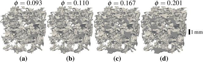
Figure 1: Fluid meshes of the limestone sample at different steps of dissolution. Sub-figures show (a) initial geometry, and (b) 1 step, (c) 2 steps and (d) 3 steps of dissolution. Fluid flow was from bottom to top during the experiments.

2.5 Computational model

The rock we consider is a cubic, sealed, elastic porous sample which can be mechanically loaded along all axes, and saturated with a steadily flowing single phase liquid. With this model, by varying the flow rate and the externally applied stress, one may obtain (1) the fluid velocity field in the pore-space of the sample at the different steps of dissolution; (2) the stress distribution in the solid space of the sample as a function of applied fluid pressure and external stress; and (3) the probability distributions of invariants of the stress tensor throughout the sample surface or volume.

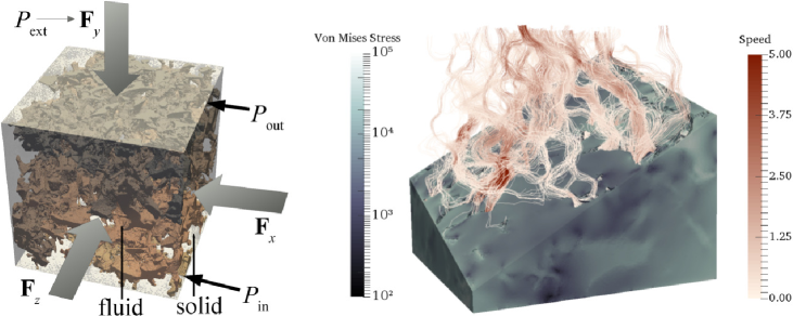
Figure 2: Left: Schematic set-up of the model. Right: Simulated 3D volume, after 3 dissolution steps, with fluid velocity streamlines and von Mises stress in the solid. The upper half has been clipped to display the fluid phase.

2.6 Implementation

The coupled fluid-solid problem is solved numerically using the FEniCS/DOLFIN framework (Logg et al., 2012a, b). The FEniCS project is a collection of software for automated solution of differential equations using the Finite Element Method (FEM), whereas DOLFIN is a C++/Python library functioning as the main user interface to FEniCS. It allows for efficient solution of differential equations requiring only a weak (variational) formulation of the problem to be specified.

2.6.1 Fluid phase

The fluid equations (7) to (11) are solved using a continuous-Galerkin method with first-order Lagrange (P₁) elements both for the velocity and pressure fields (Langtangen et al., 2002). Since this mixed-space formulation of the Stokes equations causes stability problems, as it violates the Babuska–Brezzi condition (Brenner and Scott, 2008), we use a pressure stabilization technique. This amounts to allowing a small grid-dependent compressibility which will smooth out the pressure field solution (Langtangen et al., 2002), i.e.

$$\mbox{\boldmath$\nabla$}\cdot\mathbf{v}=\delta h^{2}\mbox{\boldmath$\nabla$}^{2}P,$$ (23)

where $h$ is the element size and $\delta$ is a heuristically chosen parameter. Here, we have omitted the tildes used for scaled units for the sake of visual clarity. We verified that $\delta$ ($=0.04$) was chosen small enough for the absolute difference in inlet/outlet flux to be well below $2\text{\,}\mathrm{\char 37\relax}$, such that the mass of fluid is almost conserved.

The weak formulation of the fluid equations can thus be stated as the following: Find $\mathbf{v}\in\mathcal{V},P\in\mathcal{P}$ such that

$$\int_{\Omega_{\ell}}\left(\mbox{\boldmath$\nabla$}\mathbf{v}:\mbox{\boldmath$\nabla$}\mathbf{v}^{\prime}-P\mbox{\boldmath$\nabla$}\cdot\mathbf{v}^{\prime}+P^{\prime}\mbox{\boldmath$\nabla$}\cdot\mathbf{v}+\delta h^{2}\mbox{\boldmath$\nabla$}P\cdot\mbox{\boldmath$\nabla$}P^{\prime}\right)\mathrm{d}V\\ =-\int_{\Gamma_{\textrm{in}}}P_{\textrm{in}}\mathbf{n}\cdot\mathbf{v}^{\prime}\mathrm{d}S-\int_{\Gamma_{\textrm{out}}}P_{\textrm{out}}\mathbf{n}\cdot\mathbf{v}^{\prime}\mathrm{d}S$$ (24)

for all $\mathbf{v}^{\prime}\in\mathcal{V},P^{\prime}\in\mathcal{P}$, and $\mathbf{v}(\mathbf{x})=\mathbf{0}$ for $\mathbf{x}\in\Gamma_{\textrm{wall}}$. Here, $\mathcal{V}$ and $\mathcal{P}$ are the function spaces for velocity and pressure, respectively.

2.6.2 Solid phase

The elasticity problem is resolved similarly as the fluid phase using P₁ finite elements for the displacement field. The stress in the fluid is transferred to the boundary of the solid phase. The pressure field is given as nodal values, due to the use of first-order Lagrange elements, and can therefore be transferred directly to the solid mesh. However, the viscous stress is a derivative of the velocity field, and therefore exists as constant values on each element. Therefore, by stress reconstruction, the stress is interpolated on the boundary nodes, yielding an error of the order of the element size. To minimize this error, the mesh was refined near the fluid-solid boundaries. Additionally, the magnitude of the viscous stress is orders of magnitude smaller than that of the pressure, as shall be demonstrated in the next section, yielding an even smaller relative error in the boundary stress.

The weak problem formulation can be put as follows: Find $\mathbf{u}^{\prime}$ in $\mathcal{V}$ such that

$$\int_{\Omega_{\textrm{s}}}\mbox{\boldmath$\sigma$}[\mathbf{u}]:\mbox{\boldmath$\epsilon$}[\mathbf{u}^{\prime}]\,\mathrm{d}V\\ =-\int_{\Gamma_{\mathrm{ext}}\setminus\Gamma_{\textrm{bot}}}P_{\mathrm{ext}}\mathbf{n}\cdot\mathbf{u}^{\prime}\,\mathrm{d}S-\int_{\Gamma_{\textrm{wall}}}P\,\mathbf{n}\cdot\mathbf{u}^{\prime}\,\mathrm{d}S+\int_{\Gamma_{\textrm{wall}}}\mathbf{u}^{\prime}\cdot\mbox{\boldmath$\sigma$}_{\ell}^{\mathrm{visc}}\cdot\mathbf{n}\,\mathrm{d}S,$$ (25)

for all $\mathbf{u}^{\prime}\in\mathcal{V}$, and $\mathbf{u}(\mathbf{x})=\mathbf{0}$ for $\mathbf{x}\in\Gamma_{\textrm{wall}}$.

2.7 Probability density functions

In the simulated samples, the empirical probability density functions (PDFs), $p(\psi)$ for any given scalar field (e.g. pressure, stress invariants, fluid velocity components), $\psi$, can be calculated either on the surface or in the bulk (volume) of the sample. That is, $p(x)\,\mathrm{d}W$ gives the probability of finding the value $x$ in an arbitrary infinitesimal volume or area $\mathrm{d}W$.

For the volumetric probability distribution functions, optimal representation is achieved by weighting each nodal value by the size of its surrounding volume, similar to its Voronoi cell. For a given node $i$, this weight can be expressed as

$$w_{i}=\frac{1}{4V}\sum_{j\in\mathcal{E}_{i}}V_{j}.$$ (26)

Here, $\mathcal{E}_{i}$ is defined as the set of all mesh elements which contain node $i$, $V_{j}$ is the volume of element $j$, and $V$ is the total volume. Similarly, for the surface PDFs, the nodal weight is found by

$$w_{i}=\frac{1}{3A}\sum_{j\in\mathcal{F}_{i}}A_{j}$$ (27)

where $\mathcal{F}_{i}$ is defined as the set of all mesh facets which have node $i$ as a vertex, $A_{j}$ is the area of facet $j$, and $A$ is the total area. The PDF is then calculated by normalizing the weighted histogram of the given field. In order to minimize the effect of application of external loading, the nodes closest (within 2%) to the cubic bounding box are omitted.

3 Results

This section presents the results from the coupled fluid-solid simulations. In turn, we present the results from the fluid, and then the stress calculations in the solid due to fluid flow and porosity increase.

3.1 Main assumptions

Our results are sensitive to a series of assumptions made, mainly related to the discretization of flow in the porous samples:

• The segmentation process of solid and fluid does not unambiguously capture microporosity as some voxels could contain a fraction of solid and a fraction of porosity.

• The removal of disconnected pores and the micropores smaller than the voxel size should contribute to stress heterogeneities. Note that the removed disconnected pores represented a fraction less than 0.05 of the total pore volume.

• The meshing of the complex microstructure could be done in different ways. Note that we are here using unstructured meshes which better approximate the true microstructures than what would using e.g. a cartesian grid.

• The elastic parameters of the solid phase are assumed to be constant throughout the sample.

• The boundary conditions could have been chosen differently (e.g., strain controlled rather than stress controlled).

• The sample has a finite size, limiting the range of length scales for the observed spatial correlations.

As such, perfect agreement in comparison to experiments should not be expected. However, the meshes corresponding to snapshots of the sample at different stages of dissolution are prepared in the same way, and therefore the evolution of the distributions should hold as long as we consider viscous flow and linear elastostatics. Moreover, the largest stress concentrations are expected to be found near the biggest pores, meaning that the discretization is justified, although e.g. the “mesh porosity” is not the true porosity. Moreover, the fluid-solid solver was validated against cases where analytical expressions where available, e.g. for fluid flow in a cylindrical pipe and the stress field around a fluid-filled spherical pore. However, as the methods are rather standard and the framework is tested by the group of developers, we believe that the main sources of error lie in the points above, not in the solver itself.

3.2 Fluid flow in the pore space

Here we present the results from pure fluid flow simulations. Due to the invariance under a linear transformation described in Sec. 2.1, the results are given in scaled units. Similarly as in section 2.6.1, we have omitted the corresponding tildes for scaled units. Physical values are found by using Eqs. (6) and (14).

In Fig. 3, the simulated flow field is visualized by streamlines, i.e. integrated Lagrangian trajectories of the velocity field. As expected with increasing porosity, the flow through the sample increases. At low porosity, a few preferential flow paths are present. At higher porosities, more paths appear and cross-link with each other.

Flow through porous media is on the macroscale governed by Darcy’s law,

$${\mathbf{q}=-\frac{k}{\mu}\mbox{\boldmath$\nabla$}{P}},$$ (28)

where $\mathbf{q}$ is the flux (discharge per area) and $k$ is the permeability. Here, the flux is related to the mean velocity through the relation $\mathbf{q}=\phi\mathbf{v}$. Historically, much effort has been devoted to relating the permeability $k$ to porosity $\phi$, the most popular being the Kozeny–Carman relation commonly expressed as $k=C\phi^{3}/(1-\phi)^{2}$ (Costa, 2006; Matyka et al., 2008), where $C$ is a constant of dimension $(\textrm{length})^{2}$ related to the geometry of the porous medium. The mean absolute velocity (speed) and the mean axial velocity (parallel to the pressure gradient), are plotted as functions of porosity, $\left<v_{y}\right>(\phi)$, in the left panel of Fig. 4, and display superlinear increase with porosity. The solid lines represent power-law fittings to the data, which both yield exponents $\simeq 3$. Taking the pressure drop to be constant, the Kozeny–Carman relation predicts that the flux through any cross section of the sample $q{=\mathbf{q}\cdot\hat{\mathbf{n}}=\phi\left<v_{y}\right>}$ of a porous media should depend on porosity as

$$q\propto\frac{\phi^{3}}{(1-\phi)^{2}}.$$ (29)

This means that the average velocity should scale as $\left<v\right>\sim q/\phi\sim\phi^{2}/(1-\phi)^{2}$. The fittings shown in Fig. 4 are thus not in quantitative agreement with Kozeny–Carman relations. However, this is not unexpected, as Kozeny–Carman relations, being derived for packed beds, are usually more applicable to configurations such as high porosity sandstone, and less so for low-porosity limestone undergoing dissolution. This observation is consistent with the data presented in the right panel of Fig. 4, where permeability $k$ in physical units is plotted as a function of porosity $\phi$, and the relationship $k\sim\phi^{4}$ grows faster than the prediction from the Kozeny–Carman relation. The behaviour seen here is comparable to the data reported by Ehrenberg et al. (2006), although the magnitude is somewhat higher here, especially as dissolution progresses. The permeability calculated here, however, coincides well with the permeability reported in the original experiment (Noiriel et al., 2004).

Fig. 5 displays the measured probability distribution of fluid speed in the four volumes. The inset of Fig. 5 shows the raw (non-normalized) data, with a shift of the distribution towards higher speed as porosity is increased. The relevant features of the distributions are extracted by rescaling the speed, $v$, by the mean speed $\left<v\right>$ in each sample (displayed in Fig. 4), as shown in the main panel of Fig. 5. The distributions collapse, apart from in the tail (possibly due to the finite size of the computational meshes). As the porosity increases, the distribution approaches a stretched exponential function for large $v$,

$$p\left(\hat{v}\right)\sim\exp\left(-\alpha\hat{v}^{\beta}\right)$$ (30)

where $\hat{v}=v/\left<v\right>$, the exponent $\beta\simeq 1/2$, and the scale parameter $\alpha\simeq 0.25$. This observation is consistent with established velocity statistics for disordered porous media (Matyka et al., 2016) and the stretched exponential distribution can theoretically be inferred by considering the porous media as a collection of cylinders with exponentially distributed radii (Holzner et al., 2015).

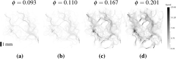
Figure 3: Streamlines of simulated velocity field in the sample at different steps of dissolution. Sub-figures (a)–(b) correspond to those in Fig. 1.

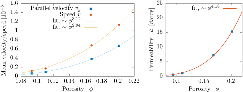
Figure 4: Left: Mean axial velocity/speed in the bulk of the fluid versus porosity in the sample, in scaled units. Right: Corresponding permeability in SI units.

Figure 5: Probability density of the fluid velocity in the pore space at different steps of dissolution. The velocity distributions are collapsed upon rescaling by the average velocity. Inset: Non-normalized distribution.

The fluid pressure distribution is shown in Fig. 6, and displays a highly heterogeneous distribution between the inlet pressure $P_{\textrm{in}}=1/2$ and the outlet pressure $P_{\textrm{out}}=-1/2$. The distribution is characterized by fluctuations (spikes) that are interpreted to be related to a heterogeneous distribution of dead-end pores. To quantify the heterogeneity in the pressure field arising from the flow, the deviation from a linear pressure profile (like what appears in hydrostatics with a constant gravitational force) can be calculated as:

$$\Delta P_{\textrm{lin}}(\mathbf{x})=P(\mathbf{x})-P_{\textrm{lin}}(\mathbf{x}),$$ (31)

where $P_{\textrm{lin}}(\mathbf{x})=1/2-y$, $y\in[0,1]$ is the scaled coordinate along the direction of the imposed pressure drop, such that $y=0$ corresponds to the inlet face, and conversely for $y=1$. The resulting distribution is shown in the inset of Fig. 6. The distribution is seen to be sharply peaked around $\Delta P_{\textrm{lin}}=0$, due to the fixed pressure at inlet and outlet, but apart from this, slightly skewed towards negative values. This indicates a geometrical asymmetry in the sample: more dead-end pores stretch from the top (low pressure) to the bottom of the samples, than the other way around.

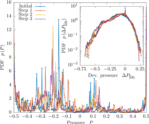
Figure 6: Fluid pressure statistics at the pore walls in the sample at different steps of dissolution.

The fluid pressure exerts a normal traction $p\hat{\mathbf{n}}$ upon the solid matrix. The viscous flow field, on the other hand, contributes to a tangential traction. The scaled viscous stress tensor is given by

$$\mbox{\boldmath$\sigma$}_{\mathrm{visc}}=\mbox{\boldmath$\nabla$}\mathbf{v}+\mbox{\boldmath$\nabla$}\mathbf{v}^{\top},$$ (32)

and to quantify this (while suppressing the influence of the boundary normal, which must be reconstructed on nodes, introducing an error of order element size) we report the distribution of $\tau$, the largest absolute eigenvalue of $\sigma_{\mathrm{visc}}$; sampled over the surface nodes (as in (Voronov et al., 2010)). The resulting distribution is shown in Fig. 7. From the latter figure, it is clear that the viscous forces are, generally, at least 1–2 orders of magnitude lower than the pressure drop, which again is lower than the base pressure $P_{0}$ and the external pressure $P_{\mathrm{ext}}$. We emphasize that this observation is independent of the value of the viscosity $\mu$, as the equations are linear and therefore only one unique solution for the stress field exists apart from a scaling (by $\Delta P$) and a shift (by $P_{0}$).

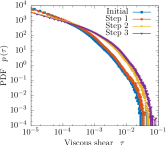
Figure 7: Fluid shear stress statistics at the pore walls in the sample at different steps of dissolution.

3.3 Stress in the porous solid

In the following, the results from calculating the state of stress in the solid due to fluid flow and porosity increase are reported. In all cases, a Poisson’s ratio $\nu=0.3$, an external pressure $P_{\mathrm{ext}}=$2.2\text{\times}{10}^{7}\text{\,}\mathrm{Pa}$$, and a base pressure $P_{0}=$1.0\text{\times}{10}^{7}\text{\,}\mathrm{Pa}$$ were used.

3.3.1 Measures of state of stress in the solid

In order to assess the impact of applied external stress on the porous sample, we consider frame-invariant quantities. Combinations of the first two invariants of the stress tensor will therefore be used ($I_{1}$ and $I_{2}$). First, the mechanical pressure is defined as

$$P_{\mathrm{mech}}=-\frac{\mathrm{tr}{{(}\mbox{\boldmath$\sigma$}{)}}}{3}.$$ (33)

Secondly, the von Mises stress (von Mises, 1913) is defined by

$$\sigma_{\textrm{vM}}=\sqrt{\frac{3}{2}\mbox{\boldmath$\sigma$}_{\textrm{dev}}:\mbox{\boldmath$\sigma$}_{\textrm{dev}}},$$ (34)

where the deviatoric stress tensor is defined by $\mbox{\boldmath$\sigma$}_{\textrm{dev}}=\mbox{\boldmath$\sigma$}+P_{\mathrm{mech}}\mathbf{I}$. The von Mises stress is commonly used to predict yielding of materials under multi-axial loading. The tightly related von Mises yield criterion states that a material starts to deform irreversibly when $\sigma_{\textrm{vM}}$ reaches a certain critical threshold $\sigma_{\textrm{yield}}$. As such, it is a measure of how close to fracturing the material is when considering a brittle material such as a rock in the first kilometers of the Earth’s crust. We note that we could as well have considered some of the common alternatives to the von Mises stress, such as the maximum principal stress (strain) i.e. the largest eigenvalue of the stress (strain) tensor, $\sigma_{1}$ (or $\sigma_{1}-\nu(\sigma_{2}+\sigma_{3})$), and the results are largely similar.

3.3.2 Influence of pressure drop over fluid on stress in the solid

Fig. 8 shows the probability distributions of $P_{\mathrm{mech}}$ in the sample before dissolution, normalized by the external pressure $P_{\mathrm{ext}}$, obtained for various fluid pressure drops $\Delta P\in[0,P_{\mathrm{ext}}]$. The distributions are peaked around $P_{\mathrm{mech}}/P_{\mathrm{ext}}=1$, with a markedly heavy tail for large $P_{\mathrm{mech}}$.

In the inset of Fig. 8 the distributions are seen to collapse by the normalization

$$\hat{P}=\frac{P_{\mathrm{mech}}-P_{\mathrm{ext}}}{P_{\mathrm{ext}}S_{\Delta P}(\frac{\Delta P}{P_{\mathrm{ext}}})}.$$ (35)

Here, $S_{\Delta P}(\Delta P/P_{\mathrm{ext}})$ is a scaling function described below.

For large $\hat{P}$, a power-law behaviour $p(\hat{P})\sim\hat{P}^{-\gamma}$, where $\gamma\simeq 5$, can possibly be observed. The support is however only over one order of magnitude and therefore other distributions might also provide good fits, e.g. a stretched exponential distribution.

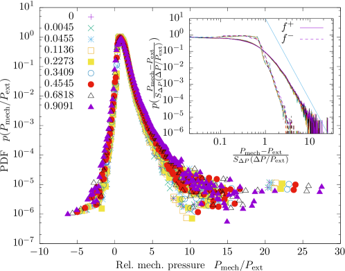
Figure 8: Probability density function of the mechanical pressure $P_{\mathrm{mech}}$ at the pore walls in the sample before dissolution, at various imposed fluid pressure drops $\Delta P$. Here, $P_{\mathrm{ext}}=$2.2\text{\times}{10}^{7}\text{\,}\mathrm{Pa}$$, $P_{0}=$1.0\text{\times}{10}^{7}\text{\,}\mathrm{Pa}$$. Inset: data collapse by rescaling. The straight line shows power-law decay $p(x)\sim x^{-5}$ as a guide to the eye. Similar plots are also found for the various dissolution steps.

The probability distributions of the von Mises stress $\sigma_{\textrm{vM}}$, corresponding to Fig. 8 are shown in Fig. 9. The distributions of $\sigma_{\textrm{vM}}$ display similar characteristics as the distributions for $P_{\mathrm{mech}}$. Scaling by $S_{\Delta P}(\Delta P/P_{\mathrm{ext}})$ yields the same data collapse as for $\hat{P}$, i.e. distributions of

$$\hat{\sigma}_{\textrm{vM}}=\frac{\sigma_{\textrm{vM}}}{P_{\mathrm{ext}}S_{\Delta P}(\frac{\Delta P}{P_{\mathrm{ext}}})}$$ (36)

are independent of $\Delta P$.

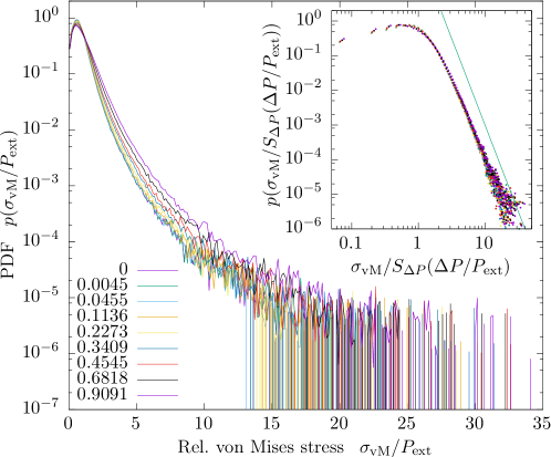
Figure 9: Probability density function of the von Mises stress $\sigma_{\textrm{vM}}$ at the pore walls in the initial step of the sample, at various imposed pressure drops $\Delta P$. $P_{\mathrm{ext}}$ and $P_{0}$ are the same as in Fig. 8. Inset: data collapse by rescaling. A power-law decay with exponent $-5$ is shown as a guide to the eye. Similar plots are also found for the various dissolution steps.

In Fig. 10, the data points show the mean of the pore-wall distribution of $\sigma_{\textrm{vM}}/P_{\mathrm{ext}}$, plotted as a function of (normalized) pressure drop. A linear least-squares fit is used to determine the scaling function:

$$S_{\Delta P}(\frac{\Delta P}{P_{\mathrm{ext}}})=0.27\frac{\Delta P}{P_{\mathrm{ext}}}+0.82.$$ (37)

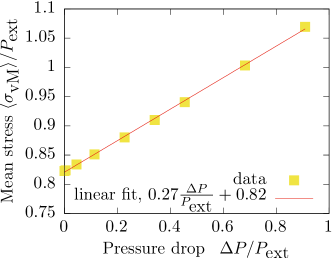
Figure 10: Mean von Mises stress as a function of the pressure drop $\Delta P$ inducing flow through the sample. The means are taken over the distributions in Fig. 9.

3.4 Influence of dissolution and increasing porosity

The probability distributions of the mechanical pressure at the pore walls of the sample at different stages of dissolution are shown in Fig. 11. Here, the pressure values used were $P_{\mathrm{ext}}=$2.2\text{\times}{10}^{7}\text{\,}\mathrm{Pa}$$, $P_{0}=$1.0\text{\times}{10}^{7}\text{\,}\mathrm{Pa}$$, and $\Delta P=0$. The peaks of the distributions are located at the same position, $P_{\mathrm{mech}}=P_{\mathrm{ext}}$, but the distributions become wider as the porosity is increased, indicating more stress concentration and more stress shadows with increasing dissolution.

To segregate the distributions of values above ($+$) and below ($-$) the peak at $P_{\mathrm{mech}}=P_{\mathrm{ext}}$, we define

$$f^{\pm}=\pm\frac{P_{\mathrm{mech}}-P_{\mathrm{ext}}}{P_{\mathrm{ext}}S(\frac{\Delta P}{P_{\mathrm{ext}}})S_{\phi}(\phi)}$$ (38)

where the scaling function $S_{\phi}(\phi)$ is defined below (see Eq. 39). As shown in the inset of Fig. 11, the resulting distributions largely collapse: the distributions of $f^{+}$ are seen to fall onto the same curve, while $f^{-}$ displays a slightly varying slope with dissolution step.

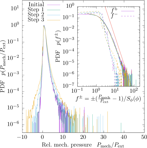
Figure 11: Probability density function of the mechanical pressure at the pore walls for all dissolution steps, at fixed $\Delta P=0$. $P_{\mathrm{ext}}$ and $P_{0}$ are the same as in Fig. 8. Inset: data collapse by rescaling. The line shows a power-law with exponent -5 as a guide to the eye. Similar plots exist for other pressure drops.

The probability distribution of the (relative) von Mises stress is plotted for the pore walls in Fig. 12 and for the solid bulk in Fig. 13. The pore-wall distributions display the same behavior and collapse by $S_{\phi}(\phi)$ as that of $f^{+}$ above. In comparison, the bulk distribution extends the suggested power-law distribution, $p(\sigma_{\textrm{vM}})\sim\sigma_{\textrm{vM}}^{-\gamma}$, $\gamma\simeq 5$, for large $\sigma_{\textrm{vM}}$.

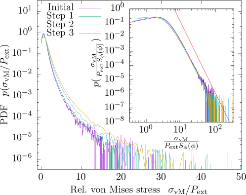
Figure 12: Probability density function of the von Mises stress at the pore walls for all samples, at fixed $\Delta P=0$. $P_{\mathrm{ext}}$ and $P_{0}$ are the same as in Fig. 8. Inset: data collapse by rescaling. Similar plots exist for other pressure drops.

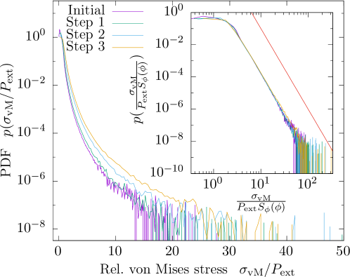
Figure 13: Probability density function of the von Mises stress in the bulk for all samples, at fixed $\Delta P=0$. $P_{\mathrm{ext}}$ and $P_{0}$ are the same as in Fig. 8. Inset: data collapse by rescaling, and a superimposed power law with exponent -5 as a guide to the eye. Similar plots exist for the other pressure drops.

The bulk averages of $\sigma_{\textrm{vM}}$, corresponding to the probability distributions shown in Fig. 13, are plotted in Fig. 14. The scaling function $S_{\phi}(\phi)$ is approximated as a fit to these points. We expect no deviatoric stress at $S_{\phi}(0)=0$, and the simplest form satisfying this is

$$S_{\phi}(\phi)=C\phi^{\beta}.$$ (39)

Here, the exponent $\beta\simeq 0.56$ yields the best fit of the experimental data using a least-square method. An even better fit would be achieved by using more complicated expressions with more fitting parameters, but for that to be justified one would also have required more than the four porosity levels available herein. Alternatively, exponential fits could be used, analogous to the compiled data of critical axial stress as a function of porosity in limestones summarized in (Croize et al., 2013, Sec. 3.1.3).

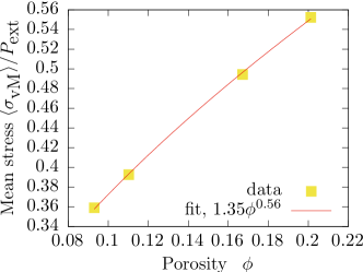
Figure 14: Bulk mean von Mises stress versus porosity. The data points correspond to the distributions in Fig. 13.

3.5 Common probability density functions

As a consequence of the above analysis, all distributions considered will collapse onto the same master curves, by the scaling relationships

$$\hat{\tilde{P}}=\frac{P_{\mathrm{mech}}-P_{\mathrm{ext}}}{P_{\mathrm{ext}}S_{\Delta P}(\frac{\Delta P}{P_{\mathrm{ext}}})S_{\phi}(\phi)},$$ (40)

and

$$\tilde{\sigma}_{\textrm{vM}}=\frac{\sigma_{\textrm{vM}}}{P_{\mathrm{ext}}S_{\Delta P}\left(\frac{\Delta P}{P_{\mathrm{ext}}}\right)S_{\phi}(\phi)},$$ (41)

where the scaling functions $S_{\Delta P}(\Delta P/P_{\mathrm{ext}})$ and $S_{\phi}(\phi)$ are given by Eqs. (39) and (37), respectively. This unified description of stress heterogeneities in the limestone sample studied here represents the main outcome of the present study.

4 Discussion

4.1 Complexity of fluid flow in a porous medium

Brown (1987) solved Reynolds equations in 2D in a synthetic rough aperture fracture and showed that for low aperture, the roughness of the walls had a significant effect, leading to flow channeling. In a porous medium, the pore structure complexity generates a wide range of flow velocities, from the fast advective flows in the main channels, to the very slow diffusive flows in dead ends where the fluid is almost stagnant and rarely mix with that in the main channels (Bijeljic et al., 2013). The pore heterogeneities have a strong effect on the long-range spatial correlations of the flux. Numerical simulations show that the distributions of the kinetic energy and the velocity in the fluid follow power laws over at least five orders of magnitude (Andrade Jr et al., 1997; Makse et al., 2000) and that the flow is correlated in space and time (Le Borgne et al., 2008), leading to intermittency (De Anna et al., 2013). Increasing the complexity of pore geometry, from a simple bead-pack porous medium to natural rock samples with micropores and microfractures increases as well the range of velocities observed in the fluid. The velocity distribution is characterized by a main peak, controlled by the pressure drop imposed on the system, and a tail of slow velocities that increases with pore network complexity (Bijeljic et al., 2013; Jin et al., 2016). Based on Lattice Boltzmann simulations, Matyka et al. (2016) proposed that the probability distribution function of fluid velocity, for velocities larger than the average fluid velocity, follows a “power-exponential” law. This is in contrast with other studies which have proposed either a Gaussian or an exponential distribution (Mansfield and Issa, 1996; Datta et al., 2013; Bijeljic et al., 2013; Lebon et al., 1996).

With regards to the speed distributions presented in Sec. 3, a stretched exponential probability density function provides a good fit for large speeds. A shifted, stretched exponential (“power-exponential”) distribution, as proposed by Matyka et al. (2016), would also be in agreement with our results, but this would require introducing another fitting parameter. Moreover, the evolving pore structure due to dissolution in our sample does not significantly alter the functional dependence of the probability density function of fluid velocities, when rescaled by the average velocity.

4.2 Coupling fluid flow and deformation

The fluid flow in the porous medium exerts both shear and normal stress on the solid walls, as shown numerically for a rough fracture (Lo and Koplik, 2014). Because of the complexity of the porous medium, additional complexity of the flow pattern exists and long range correlations in the stress distribution at the solid interface emerge.

Flow-induced stresses have been modeled for several biological applications where porosity of the medium was quite high (above 80 %) and the solids were very soft. Under these conditions, numerical simulations indicate that the fluid viscous stress at the pore walls follows a gamma distribution (Voronov et al., 2010). Numerical models of fluid flow in highly deformable elastic porous media indicated that, as the elastic solid deforms under flow, the relationship between pressure drop and flux becomes non-linear and saturates for large pressure gradients (Hewitt et al., 2016). Hysteresis due to the coupling between fluid and solid can emerge (Guyer and Kim, 2015). Pham et al. (2014) calculated the stress exerted by a fluid around a spherical solid using Lattice Boltzmann simulations, and the existence of areas with stress concentration on the solid, and log-normal stress distribution was observed. However, in all these studies, the porosity was quite large and/or the solids were very soft and relevant for bioengineering applications. This renders comparison with solids that are stronger and with lower porosity, such as rocks, challenging.

In rocks, elastic deformations are quite small, usually below one percent, before irreversible strain occurs. Depending on stress and the mechanisms of irreversible deformation, such as closure and opening of microcracks or pore collapse, the relationship between porosity and permeability evolves, controlling the pore pressure gradient (David et al., 1994). Under loading, the microscale heterogeneities control both the initiation of microcracks and the overall strength of the material. Using a 2D discrete element modeling approach applied to a granite rock, Lan et al. (2010) showed a difference between geometrical heterogeneities (i.e. difference of grain size), which control the nucleation of microfractures and initiation of damage, and strength heterogeneities at the grain contacts (i.e. elastic stiffness), which control the overall strength of the solid under uniaxial loading. In these simulations, the stresses inside the grains show a normal distribution for both the maximum and the minimum principal stress, with an average value which corresponds to the external loading. Conversely, the normal stress at grain contacts shows a bimodal distribution. Some contacts are under tensile normal stress conditions and provide sites for the nucleation of extensional microfractures.

The evolution of elastic parameters and permeability during small elastic deformations of a Bentheim sandstone was experimentally measured and successfully modeled using X-ray microtomography images where unstructured meshes were built (Jasinski et al., 2015). The effect of fluid viscosity on the effective elastic properties of rocks and the attenuation of elastic waves was studied in (Saenger et al., 2011) by solving the dynamic elastic equation in 3D rock samples imaged with X-ray microtomography. Other researchers have simulated deformation of calcium carbonates with a back-coupling to flow through dissolution (Pereira Nunes et al., 2016) and precipitation (Jiang and Tsuji, 2014), although without accounting for the stress distribution in the solid matrix. In the present work, the fluid-solid coupling is only one-way and therefore the effect of flow on changing pore-space geometry can not be assessed.

By considering probability density functions of bulk and pore-wall properties, the results presented in Sec. 3 show that for a steadily flowing fluid in the pore space of a limestone, the dominating force from the fluid stems from the base pressure in the solid, as the viscous force generated by the fluid is generally orders of magnitude lower. This implies that under such conditions, the viscous stress is of minor importance. Moreover, the stress distributions are controlled by the pressure drop $\Delta P$ in a simple manner. In particular, the position of the tail of the distributions of stress in the sample may ultimately depend on the maximum difference between external and internal pressure. This broad tail, with a power-law decay with a quite strong exponent of -5, has the following consequence: a slight increase in fluid pressure or a small amount of dissolution will significantly increase the number of locations in the solid where the von Mises criteria (or another failure criteria) will be reached. A consequence of such behavior is the following. It is known that the injection or removal of fluid at depth can to trigger induced seismicity (Talwani and Acree, 1984). Recent field observations at the outcrop scale show that a small fluid injection can trigger microearthquakes at some distance from the injection point (Guglielmi et al., 2015). If they can be extended to other kinds of rocks, our results, with a heavy power-law tail of stress heterogeneities, show that a small change in fluid pressure can drive a significant volume of the rock towards failure. The nature of microstructural heterogeneities and their relationships to fluid flow and stress would then provide an additional explanation of induced seismicity.

Whether the observed self-similarity persists if the porosity is increased beyond the range considered here, is an open question, and could be assessed e.g. by using tomography data from experiments where more dissolution is performed. However, in the Earth’s crust failure would occur before reaching a high porosity, which is what happens for example in karst with the formation of caves. Further, how the distribution changes if such failure occurs, i.e. the stress heterogeneity leads to fractures, is an interesting point in question. We expect the self-similar behaviour will reach its end at latest when the first failure occurs, as the solid matrix will then reorganize itself.

5 Conclusion

We have in this work computationally studied how an evolving microstructure influences fluid flow in the pore space of a rock, and how fluid flow influences the state of stress in the solid phase. We have considered a limestone which has been scanned at four stages of dissolution using X-ray microtomography.

Steady incompressible laminar fluid flow in the sample at each stage of dissolution was computed by solving Stokes’ equations. By assuming negligible displacement of the fluid-solid boundary due to elastic deformation, the stress field from the fluid enters as a boundary condition on the solid, yielding a one-way numerical coupling. Both the fluid and the solid problems were solved numerically using the finite element method through the FEniCS/DOLFIN framework.

Our main finding is that, as the rock is dissolved, and as the pressure drop driving the fluid flow is increased, the distribution of heterogeneous stress in the sample evolves in a self-similar manner. In particular, the probability distributions of the mechanical pressure and the von Mises stress can be collapsed onto the same curve by a normalization. The common master curves display a broad distribution, with a suggested power-law tail for high stresses. The broad tail shows that the rock is very sensitive to small perturbations, and a slight fluid pressure increase locally would drive a significant number of local heterogeneities toward failure. We propose that this heavy tail can be used as a simple criterion for the integrity of porous rocks.

Whether the observed self-similar evolution is restricted to dissolution processes remains to be answered. For example, do other morphology-changing processes, such as fracturing or precipitation (lowering porosity) evolve similarly? A more fundamental question is related to identifying the link between pore geometry and the velocity distribution/stress distribution. Future work will include a back-coupling from solid deformation to fluid flow, yielding transient dynamics of fracture and/or precipitation–dissolution processes.