The VLT-FLAMES Tarantula Survey

Abstract

Aims. We estimate physical parameters for the late-type massive stars observed as part of the VLT-FLAMES Tarantula Survey (VFTS) in the 30 Doradus region of the Large Magellanic Cloud (LMC).

Methods. The observational sample comprises 20 candidate red supergiants (RSGs) which are the reddest (($B-V$) $>$ 1 mag) and brightest ($V$ $<$ 16 mag) objects in the VFTS. We use optical and near-IR photometry to estimate their temperatures and luminosities, and introduce the luminosity–age diagram to estimate their ages.

Results. We derive physical parameters for our targets, including temperatures from a new calibration of $(J-K_{\rm s})_{0}$ colour for luminous cool stars in the LMC, luminosities from their $J$-band magnitudes (thence radii), and ages from comparisons with state-of-the-art evolutionary models. We show that interstellar extinction is a significant factor for our targets, highlighting the need to take it into account in analysis of the physical parameters of RSGs. We find that some of the candidate RSGs could be massive AGB stars. The apparent ages of the RSGs in the Hodge 301 and SL 639 clusters show a significant spread (12–24 Myr). We also apply our approach to the RSG population of the relatively nearby NGC 2100 cluster, finding a similarly large spread.

Conclusions. We argue that the effects of mass-transfer in binaries may lead to more massive and luminous RSGs (which we call ‘red stragglers’) than expected from single-star evolution, and that the true cluster ages correspond to the upper limit of the estimated RSG ages. In this way, the RSGs can serve as a new and potentially reliable age tracer in young star clusters. The corresponding analysis yields ages of 24${}^{+5}_{-3}$ Myr for Hodge 301, 22${}^{+6}_{-5}$ Myr for SL 639, and 23${}^{+4}_{-2}$ Myr for NGC 2100.

1 Introduction

Multi-epoch spectroscopy of an unprecedented sample of hot, massive stars in the 30 Doradus region of the Large Magellanic Cloud (LMC) was obtained by the VLT-FLAMES Tarantula Survey (VFTS, Evans et al. 2011, hereafter Paper I). To try to obtain an unbiased view of the massive-star population of 30 Dor, no restrictions on colour were employed in the VFTS target list, so as to potentially include heavily reddened O-type stars that were expected to be present in the region. The resulting observed sample therefore included spectra of 91 later-type stars in the region (with spectral types ranging from early A to M, see Table 3 of Paper I), plus spectra for an additional 102 stars thought to be mostly cool foreground stars. Among these two sets of cool stars are $\sim$20 stars that are known red supergiants (RSGs) or new candidate RSGs. Here we investigate their stellar parameters and evolutionary status, and discuss their ages in the context of the age of the 30 Dor region and its component stellar groups.

RSGs represent the final evolutionary stage of most massive stars before core-collapse. They also represent the physically largest evolutionary phase possible for single stars, making them critical for understanding the total fractions, mass ranges, and evolutionary states of interacting massive binaries (Levesque 2017). Indeed, the high incidence of interacting massive binaries (Sana et al. 2012) is expected to lead to about half of the type II supernova population resulting from post-interaction or merged stars (Podsiadlowski et al. 1992, Zapartas et al. in prep.) and to delayed supernovae relative to single star evolution (e.g. Zapartas et al. 2017). However, our understanding of these stars is hindered as correct determination of their physical parameters is still challenging due to the many uncertainties associated with modelling their complex atmospheres and winds (e.g. Massey et al. 2005; Levesque 2010; Davies et al. 2013). The evolutionary history of RSGs also depends on metallicity, initial mass, and probably binarity. The RSGs found in two clusters in the 30 Doradus region, Hodge 301 (Hodge 1988) and SL 639 (Shapley & Lindsay 1963), are particularly interesting because they enable study of two samples of RSGs that are each presumably coeval, as discussed later.

The wavelength coverage of the VFTS spectra was tailored to the analysis of OB-type stars (see Paper I). While useful to classify late-type stars, the coverage is not sufficient to estimate effective temperatures for RSGs, so we have resorted to photometric methods to investigate the physical properties of our sample. There are a number of different approaches discussed in the literature, so we briefly review these to assess potential advantages or drawbacks. A radial-velocity (RV) analysis of the VFTS spectroscopy of the sample is presented in a companion paper (Patrick et al. submitted).

This paper is organised as follows: Section 2 introduces our observational sample and Section 3 uses three photometric techniques to estimate the physical parameters of each star. We discuss our results in Section 4, with brief conclusions presented in Section 5.

2 Observational sample

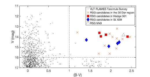
Figure 1: Colour–magnitude diagram for the VFTS targets, highlighting the candidate RSGs studied and their membership of (or association with) the Hodge 301 and SL 639 clusters. The photometric criteria ($V$ $<$ 16 mag, $(B-V)$ $>$ 1 mag) are indicated by the dashed lines.

The VFTS included observations of 91 targets with spectral types ranging from A through to M (see Table 3 in Paper I). To select candidate RSGs for this study (and that of Patrick et al.) we used photometric criteria of ($B-V$) $>$ 1 mag and $V$ $<$ 16 mag, as shown in the colour–magnitude diagram in Fig. 1.

Apparently foreground stars with RV $<$ 100 km s^-1 were excluded from the VFTS sample by inspection of the spectra at the outset of the project (see Section 2.2.2. of Paper I). At that stage, we also omitted a small number of cool stars that appeared to have RVs consistent with membership of the LMC but with very low signal-to-noise (S/N) spectra. In the context of this study and the RV analysis by Patrick et al. (submitted), these low S/N spectra can still provide new insights, so we supplemented the primary VFTS targets with three stars that were omitted from Paper I but that appear to be members of the LMC. For future reference the full listing of the 102 previously discarded targets is given in Table LABEL:rejects, where they are given IDs of the form 2xxx to distinguish them from the primary VFTS catalogue.

Given our focus on Hodge 301 and SL 639 we also include photometry of RSG WB97#5 (Walborn & Blades 1997; Grebel & Chu 2000) in Hodge 301, which was not observed in the VFTS due to crowding in the core of this cluster. For completeness, we also consider the brightest RSG in the region, Mk 9 (Melnick 1985); by chance this was not included in the VFTS sample due to the high density of targets in and around R136 (which limited the fibre allocations).

The observational parameters of the resulting 20 candidate RSGs are summarised in Table 1. They can loosely be characterised as belonging to one of three groups: associated with the older clusters Hodge 301 and SL 639, (loosely) associated with the young star-forming region NGC 2060, and those in the field with no clear association. The locations of our sample in the 30 Dor region are shown in Fig. 2, with the spatial extent of the four clusters as defined by Evans et al. (2015) also shown.

Table 1 includes the mean RVs for each target from cross-correlation of the LR02 spectra (3960–4564 Å) with a synthetic spectrum from a marcs model atmosphere (see Patrick et al. submitted). All but one have RVs consistent with the systemic line-of-sight velocity of the 30 Dor region. The exception is VFTS 793, with a significantly lower velocity of RV $=$ 187 $\pm$ 1 km s^-1. The parallax ($p$) for VFTS 793 from the Gaia Data Release 2 (DR2) catalog (Gaia collaboration, Lindegren et al. 2018) is $p$ $=$ 0.1874 $\pm$ 0.016 mas, giving a distance modulus of 13.63 mag ($\approx$5.3 kpc). As such, we consider this object as a foreground giant and exclude it from our subsequent analysis.

The RV estimates for the members of each cluster are in good agreement, and help to reveal three further stars which are potentially associated with the clusters. VFTS 236 is at a projected distance of only 14 pc from Hodge 301, and its RV estimate is near-identical to those for VFTS 281 and 289. Similarly, the estimates for VFTS 852 and 2090 (at projected distances of $\sim$36 pc) are in good agreement with those for the two members of SL 639, see Patrick et al. (subm.) for statistical arguments regarding membership of the respective clusters. For comparison, the mean RV for the remaining ten stars in Table 1 (excl. VFTS 793) is 271 $\pm$ 15 $\mbox{km s}^{-1}$, i.e. the three spatially-outlying stars from the clusters appear kinematically associated with them cf. the general velocity dispersion of the cool stars across the region. The radius adopted for these two clusters by Evans et al. (2015) was a (knowingly conservative) ad hoc assumption of 20^′′ to delineate the sample to investigate the cluster ages. That we find potentially associated stars at larger radii is not unexpected, and is analogous to the RSG population in the nearby NGC 2100 cluster, which extends out to radii of nearly 30 pc with a similarly small velocity dispersion (Patrick et al. 2016). Thus, we consider these three stars (VFTS 236, 852, 2090) as candidate members of their respective clusters.

Our analysis used magnitudes from the following sources: $V$-band from Paper I, $I$-band from DENIS (Cioni et al. 2000) and $JHK_{\rm s}$-bands from 2MASS (Skrutskie et al. 2006). Significant spectral variability is thought to occur in only a relatively small fraction of RSGs in the LMC (see discussion by Bonanos et al. 2009). However, semi-regular photometric variability is seen in many RSGs and to account for the fact that we are using heterogeneous catalogues we adopted systematic photometric uncertainties of 0.2 mag in the $V$-band and 0.1 mag in the near-IR bands (based on the average variability of well-studied RSGs, e.g. Josselin et al. 2000; Kiss et al. 2006; Yang & Jiang 2011, 2012). We caution that a small fraction of RSGs can undergo long-term variations of a magnitude or more in the visible, which may influence some of our results based on $V$-band magnitudes (cf. the near-IR), but our near-IR analysis should be robust to such effects.

3 Determination of physical parameters

3.1 Effective temperatures & luminosities of red supergiants

The effective temperatures of RSGs have been subject to a number of substantial studies in recent years. Levesque et al. (2005) used optical spectrophotometry and revised marcs models to arrive at an effective temperature scale that was approximately 10% warmer than previously published values. They used this result to produce a ‘$V-K$’ calibration of the effective temperature scale of RSGs and applied this to stars in the Magellanic Clouds (Levesque et al. 2006, 2007). However, Davies et al. (2013) argued that such optical analyses are strongly influenced by the strong TiO bands in RSG spectra, which are thought to be formed further out in the atmosphere, yielding lower temperatures than spectral fits to the optical and near-IR continuum. The ‘$V-K$’ method shows good agreement with theory in the derived temperatures for bright field RSGs in the Magellanic Clouds (Levesque et al. 2006, 2007). However, in the case of the 30 Dor sample that have substantially higher extinctions (cf. Table 1) the application of this method requires a precise extinction determination for each target. Clearly, the ‘$V-K$’ calibration will be more sensitive to uncertainties in the $V$-band extinction, than to uncertainties in the $K_{\rm s}$-band.

Near-IR photometry can be useful to identify RSGs for spectroscopic follow-up (e.g. Patrick et al. 2015), for example, via their $J-K$ colours (Nikolaev & Weinberg 2000). However, it has not generally been used on its own to estimate physical parameters. Motivated by the above complications in using $V-K$, we investigated the use of near-IR photometry to estimate temperatures for our sample. These two approaches are now discussed below, as well as the use of single-band photometry to estimate stellar luminosities independently of T_eff, as advocated by Davies et al. (2013).

Table 1: Observational properties of the late-type sample from the VLT-FLAMES Tarantula Survey (VFTS).

VFTS ID	$\alpha$	$\delta$	$V$	$I$	$J$	$H$	$K_{\rm s}$	AV	RV (LR02)	Notes
	(J2000)	(J2000)	(mag)	(mag)	(mag)	(mag)	(mag)	(mag, $r\,<\,$1$\aas@@fstack{\prime}$5)	(km s-1)
023	05 37 16.08	$-$69 08 52.86	15.63	13.44	11.814	10.814	10.484	2.42 $\pm$ 0.46	267.3 $\pm$ 2.6
081	05 37 35.99	$-$69 12 29.93	13.71	11.69	10.279	9.363	9.067	1.96 $\pm$ 0.25	283.2 $\pm$ 2.4	K4 (GF15)
198	05 37 54.64	$-$69 09 03.36	14.02	11.82	10.301	9.391	9.067	1.67 $\pm$ 0.52	255.0 $\pm$ 1.4	K4.5 Iab (GF15)
222	05 38 00.57	$-$69 09 41.64	14.86	12.93	11.456	10.588	10.312	1.40 $\pm$ 0.33	250.4 $\pm$ 1.0
236	05 38 06.61	$-$69 03 45.25	13.80	11.90	10.536	9.677	9.413	1.14 $\pm$ 0.25	258.5 $\pm$ 0.9	Hodge 301 candidate
275	05 38 16.00	$-$69 10 11.39	14.22	11.47	9.308	8.336	7.867	1.28 $\pm$ 0.22	286.7 $\pm$ 1.0	M4 (GF15), M1.5 (L07)
281	05 38 16.68	$-$69 04 14.09	13.99	11.38	9.786	8.906	8.552	1.14 $\pm$ 0.25	260.3 $\pm$ 1.6	Hodge 301 member
289	05 38 17.64	$-$69 04 12.03	13.96	12.13	10.848	10.011	9.722	1.14 $\pm$ 0.25	258.1 $\pm$ 1.7	Hodge 301 member
341	05 38 26.69	$-$69 08 52.70	14.02	11.66	9.782	8.754	8.340	2.18 $\pm$ 0.81	278.7 $\pm$ 2.9	K5 (GF15)
655	05 38 51.19	$-$69 06 41.29	15.13	13.02	11.497	10.598	10.260	2.00 $\pm$ 0.55	282.0 $\pm$ 0.9
744	05 39 07.13	$-$69 01 52.77	15.63	13.23	11.688	10.668	10.363	1.92 $\pm$ 0.91	248.2 $\pm$ 3.1
793	05 39 28.18	$-$69 05 50.49	13.58	12.33	11.422	10.735	10.616	1.75 $\pm$ 0.30	187.4 $\pm$ 1.0	Foreground, K I (GF15)
828	05 39 39.41	$-$69 11 52.05	14.52	11.60	9.864	8.965	8.524	2.50 $\pm$ 0.30	247.0 $\pm$ 1.1	SL 639 member, M (GF15)
839	05 39 41.78	$-$69 11 31.01	14.64	12.03	10.280	9.352	8.935	2.50 $\pm$ 0.30	248.0 $\pm$ 1.2	SL 639 member
852	05 39 52.39	$-$69 09 41.26	14.30	12.21	10.682	9.733	9.407	2.15 $\pm$ 0.21	243.2 $\pm$ 3.0	SL 639 candidate
2002	05 37 13.50	$-$69 08 34.65	14.21	11.57	9.720	8.721	8.292	2.46 $\pm$ 0.55	284.3 $\pm$ 3.4	M3 (GF15)
2028	05 37 58.67	$-$69 14 24.07	13.27	11.06	9.532	8.716	8.383	1.20 $\pm$ 0.33	274.0 $\pm$ 2.5	G5 Ia (GF15)
2090	05 40 07.01	$-$69 11 41.50	14.88	12.65	11.035	10.067	9.717	2.50 $\pm$ 0.30	247.1 $\pm$ 1.0	SL 639 candidate
WB97 5	05 38 17.01	$-$69 04 00.98	13.60	11.58	10.077	9.193	8.866	1.17 $\pm$ 0.24	…	Hodge 301 member
Mk 9	05 38 48.48	$-$69 05 32.58	13.62	10.86	9.173	8.297	7.869	1.92 $\pm$ 0.30	…	M3.5 Ia (GF15)

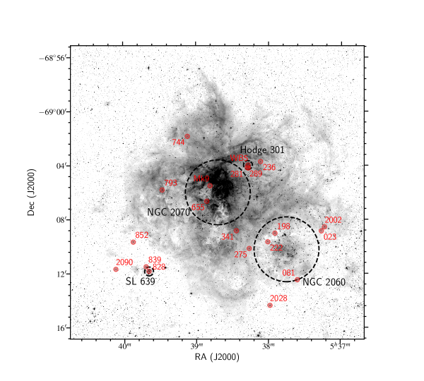
Figure 2: Spatial distribution of the late-type stars in 30 Doradus and extent of the NGC 2070, NGC 2060, Hodge 301 and SL 639 clusters (as adopted by Evans et al. 2015, in which the larger clusters have indicative diameters of $\sim$70 pc and the smaller, older clusters have diameters of $\sim$9.5 pc). The image is from a $V$-band mosaic taken with ESO’s Wide Field Imager on the 2.2 m telescope at La Silla (under programme 076.C-0888).

3.1.1 V – K method

We initially estimated stellar parameters using the $V$ $-$ $K$ method from Levesque et al. (2005). Aside from the issues arising from using the TiO bands, we were interested to investigate this approach for comparison with other methods. As discussed, many of our sources have high extinction, so the most critical aspect with this method is to obtain reliable estimates for the optical extinction ($A_{V}$) to each target. For this purpose we used the mean reddening of (morphologically normal) O-type stars from Walborn et al. (2014) within a search radius of 1$\aas@@fstack{\prime}$5 of each candidate RSG (typically yielding 3–5 O-type stars per target). Given estimates of $E(B-V)$ for each target and adopting a ratio of total-to-selective extinction of $R_{V}$ $=$ 4.48 $\pm$ 0.24 (De Marchi et al. 2016), we estimated the line-of-sight extinction from $A_{V}$ $=$ $E(B-V)$ $\times$ $R_{V}$. The resulting extinction estimates and their uncertainties are listed in Table 1, where the values for most of the stars in Hodge 301 and SL 639 are identical simply because they are located so close to each other. Our estimated reddening toward Hodge 301 is in good agreement with the mean value of $E(B-V)$ $=$ 0.28 $\pm$ 0.05 from Grebel & Chu (2000).

We then used the calibrations of T_eff and bolometric corrections (BC_K) as a function of $V-K$ colour from Levesque et al. (2006, 2007). Their technique was based on fits to spectrophotometric observations of 36 RSGs in the LMC with synthetic spectra calculated from marcs atmosphere models (Gustafsson et al. 2003, 2008). The general precision of the method, i.e. the standard deviation of temperature differences between the marcs model fitting of the TiO region and the $V$ $-$ $K$ calibration is $\sim$100 K (see Levesque 2017).

To apply this technique to our sample we dereddened our sources using: $(V-K_{\rm s})_{0}$ $=$ $(V-K_{\rm s}$) $-$ 0.87 $A_{V}$, based on $A_{K}$ $=$ 0.13 $A_{V}$ (from the $R_{V}$ dependent extinction law of O’Donnell 1994, adoping $R_{V}$ $=$ 4.48), then calculated bolometric magnitudes from: $M_{\rm Bol}$ $=$ $K$ $-$ 0.13 $A_{V}$ $-$ DM $+$ BC_K, in which we adopt a distance modulus to the LMC of 18.5 mag. Estimates of T${}_{\rm eff}^{(V-K)}$ and L^(V-K) using their calibration are given in Table 3.

3.1.2 J – K method

Bessell & Wood (1984) presented bolometric corrections for late-type stars in the Clouds based on the $(J-K_{\rm s})$ colours for 90 stars. Dorda et al. (2016) employed this relation for RSG stars, entailing transforming the photometric system and then dereddening the colours for each target. They then used the results from Bessell & Wood (1984) to estimate BC_K, thence luminosity (L^(J-K)), analagous to the method in Section 3.1.1. We also investigate this approach for our sample.

The $(J-K_{\rm s})$ colours also appear to be useful to estimate effective temperatures of RSGs. Tabernero et al. (2018) presented temperatures for 217 RSGs in the LMC from fits to spectra of the 8400–8800 Å region using synthetic spectra calculated from 1D Local Thermodynamic Equilibrium (LTE) kurucz models (Mészáros et al. 2012). This region is relatively free of telluric and molecular bands, and includes several Fe I lines as well as the strong Calcium Triplet lines in RSGs, e.g. Fig. 2 from Tabernero et al. (see also, e.g. Britavskiy et al. 2014). As shown in Fig. 3, with the benefit of the large sample of results from Tabernero et al., a good correlation between T_eff and $(J-K_{\rm s})$ is revealed, with a linear fit (valid for 0.8 mag  $<$ $(J-K_{\rm s})$ $<$ 1.4 mag) described by:

$${\rm T}_{\rm eff}^{(J-K)}=-791\times(J-K_{\rm s})_{0}+4741,$$ (1)

with a standard deviation of $\sigma$(T${}_{\rm eff})$ $=$ 140 K. To use this relation it is necessary to deredden the colour, i.e. $(J-K_{\rm s})_{0}$ $=$ $(J-K_{\rm s})$ $-$ $E(J-K)$. From Schlegel et al. (1998) the near-IR reddening can be derived as $E(J-K)$ $=$ 0.535$E(B-V)$, assuming $R_{V}$ $=$ 3.1, with the reddening value of $E(B-V)$ specific to each target. A calibration of T_eff vs. $(J-K_{\rm s})_{0}$ from Neugent et al. (2012) is also shown in Fig. 3, which was derived using a sample of yellow SGs ($(J-K_{\rm s})$ $<$ 0.9 mag) and candidate RSGs in the LMC. Their hotter sample and their fits with varying log $g$ values (cf. the constant value of zero adopted by Tabernero et al.) both contribute to the difference in slopes.

Our estimates of temperature (T${}_{\rm eff}^{(J-K)}$, from Eqn. 1) and luminosity (L^(J-K)) from this method are given in Table 3, in which the uncertainties on the former are the dispersion of 140 K in the calibration combined with the uncertainty in T_eff arising from the uncertainty on the extinction. For consistency, the latter includes use of the same $E(J-K)$ relation as for the Tabernero et al. sample (although using $R_{V}$ $=$ 4.48 would lead to only a small change in colour, with minimal impact on T_eff cf. the spread in Fig. 3).

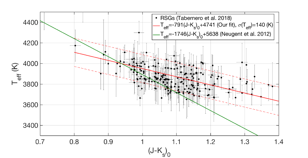
Figure 3: Effective temperature (T_eff) vs. $(J-K_{\rm s})_{0}$ colour for the 217 RSGs in the LMC from Tabernero et al. (2018). The red line is our linear fit to their data and the green line shows a previous calibration from a sample of yellow SGs and RSGs by Neugent et al. (2012).

3.1.3 Single-band photometry

Empirical luminosity calibrations for single-band photometry of RSGs in the LMC and SMC were given by Davies et al. (2013, their Table 4). These calibrations assumed that the bolometric correction for the RSGs is constant for each given photometric band, a consequence of the near-uniform temperatures (to $\pm$100 K) of the stars analysed by Davies et al. To investigate this method for our sample we used the available $I$-, $J$- and $K_{\rm s}$-band magnitudes, allowing us to test for the effects of extinction and to understand which band gives the most robust results. For each band ($x$), we calculated the absolute magnitude for each target as: $M_{x}$ $=$ $m_{x}$ $-$ $A_{x}$ $-$ DM, with estimates of extinction of: $A_{I}$ $=$ 0.54 $A_{V}$, $A_{J}$ $=$ 0.32 $A_{V}$, $A_{K}$ $=$ 0.13 $A_{V}$, based on the adopted value of $R_{V}$=4.48 by applying the extinction law of O’Donnell (1994). While the extinction coefficient for each band depends on spectral type (van Loon et al. 2003), taking into account that all our targets have K or early M spectral types, the resulting difference in extinction is very small and we did not take it into account.

The resulting luminosity estimates (L^(I), L^(J), and L^(K)) are listed in Table 3. The internal dispersion of the three bands for our stars was $\sigma$(log(L/L_☉)) $=$ 0.05, although we note the calibration itself was limited to a sample of 19 RSGs in the Clouds (Davies et al. 2013). As pointed out by Davies et al. (2013) a major advantage of this approach is that the resulting stellar luminosities are relatively insensitive to errors in the effective temperature since we are near the flux maximum of the spectral energy distribution. The resulting uncertainties in the luminosities for each method listed in Table 3 consist of the internal dispersion of the methods together with the individual uncertainties on the $A_{V}$ and $R_{V}$ values.

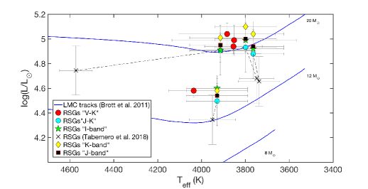
Figure 4: Hertzsprung–Russell diagram showing results for four stars from the photometric methods discussed in Section 3 compared with published results from Tabernero et al. (2018, linked by the dashed lines to our results).

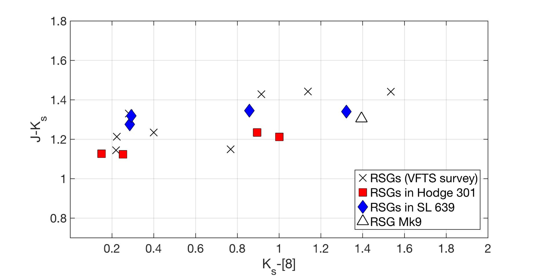
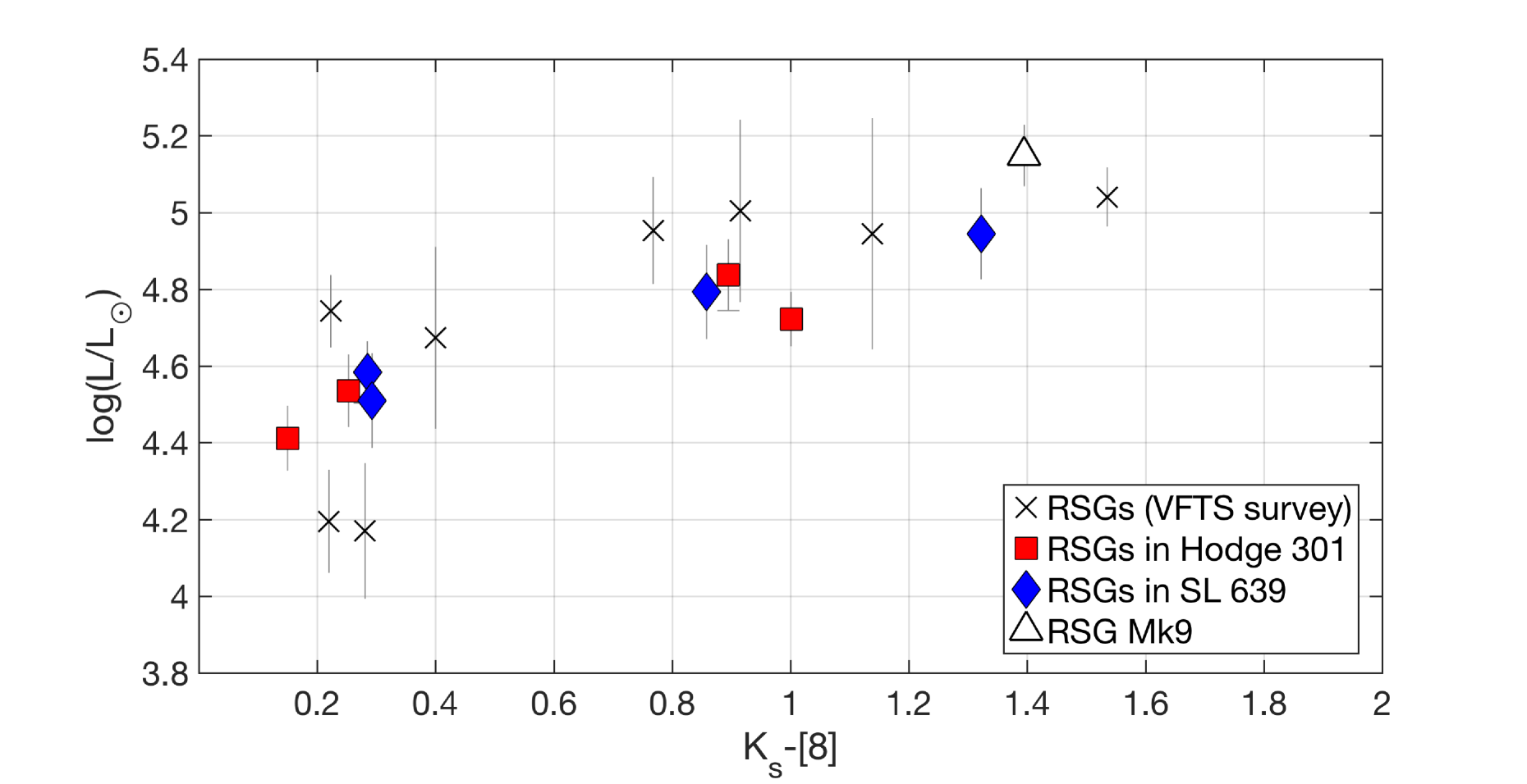
Figure 5: Upper panel: $(J-K_{\rm s})$ vs. $(K_{\rm s}-[8.0])$ diagram for our sample. Lower panel: Luminosity vs. $(K_{\rm s}-[8.0])$ for the same stars.

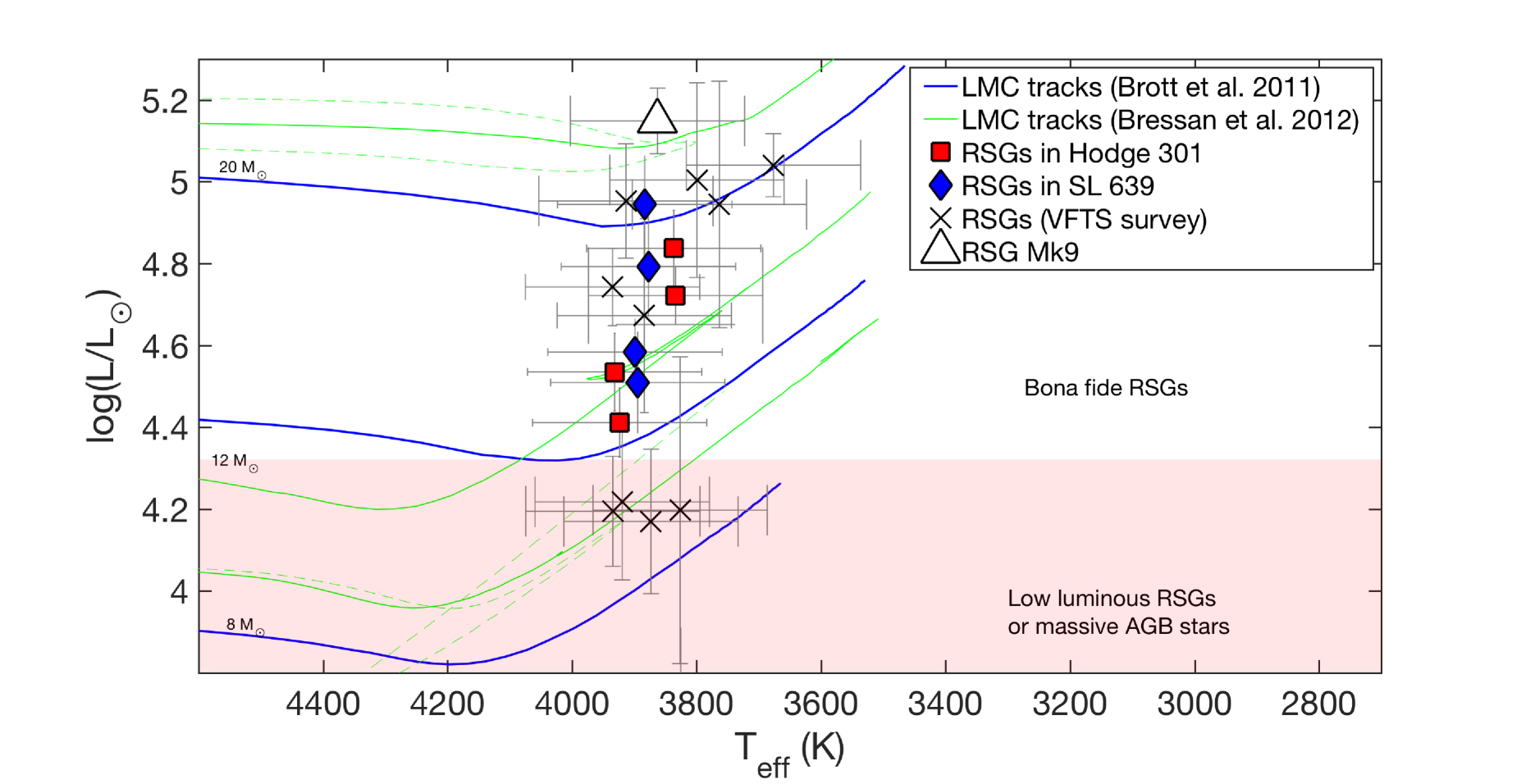
Figure 6: Hertzsprung–Russell diagram for our targets, in which temperatures were estimated using the $J$ $-$ $K$ approach and luminosities estimated from $J$-band magnitudes. The classifications of the targets based on our analysis are highlighted by the comments and filled region. Blue loops in the parsec evolutionary models from Bressan et al. (2012) are marked by dashed lines (see text for details).

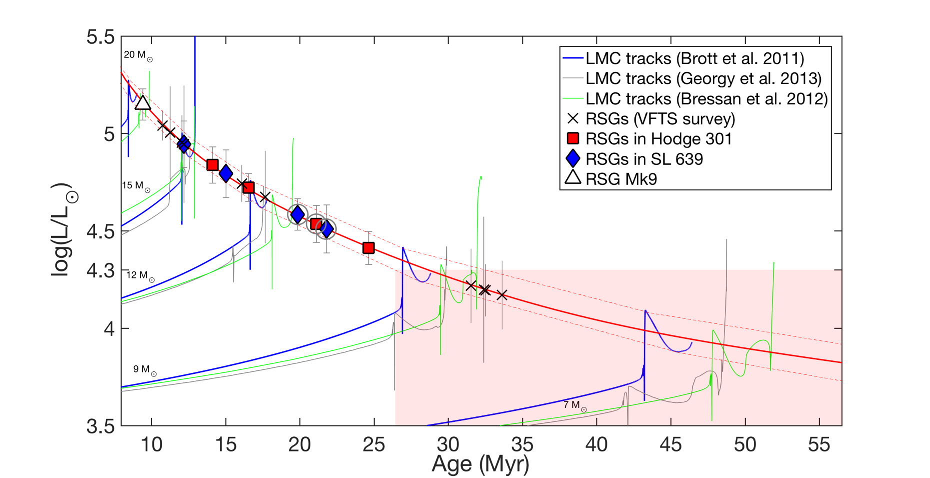
Figure 7: Luminosity–age diagram for our sample of RSGs compared with evolutionary tracks for LMC metallicity from Brott et al. (2011), Georgy et al. (2013) and Bressan et al. (2012). The luminosities that RSGs are expected to occupy during the He-burning phase from the Brott et al. (2011) models are shown by the red dashed lines. The red solid line corresponds to a fourth-degree polynomial interpolation of the RSG region: Age $=$ $-$0.413L⁴$-$3.868L³+128.081L²$-$796.823L+1534.899 (Myr), where L is in units of log(L/L_☉). This interpolation can be used for ages of 8 to 55 Myr. The filled red area highlights ages that would be excluded by a luminosity threshold of log(L/L_☉) = 4.3 dex being adopted as a lowest RSG luminosity limit according to Fig.6. Using our derived stellar luminosities we can place each star in the RSG region to read off an evolutionary age, or age range, as shown. The cluster candidates are marked by grey circles.

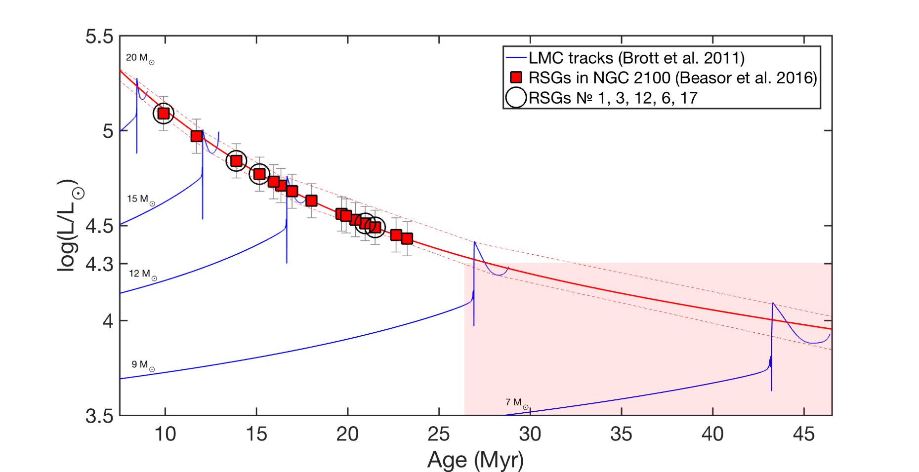
Figure 8: Luminosity–age diagram as in Fig. 7 but using results from Beasor & Davies (2016) for RSGs in the relatively nearby NGC 2100 cluster. The five most distant RSGs from the visual cluster centre are highlighted to investigate potential spatial effects (see text for discussion).

3.1.4 Comparison of the three methods

Estimates of temperature and luminosity for four of our targets are available from Tabernero et al. (2018). Our results from the three methods outlined above are compared with theirs in the Hertzsprung–Russell (H–R) diagram in Fig. 4. Tabernero et al. calculated luminosities using the same J–K method as here, but without correcting for extinction, hence our estimates are all larger than theirs. Note that the three methods explored here give similar luminosity estimates once extinction is taken into account. Indeed, for our heavily reddened sample, it is critical to correctly account for interstellar extinction to obtain reliable estimates of their luminosities.

The star with a large difference in T_eff cf. Tabernero et al. is VFTS 2028 (T${}_{\rm eff}^{(J-K)}$ $=$ 3914 $\pm$ 143 K here, cf. the published value of 4572 $\pm$ 75 K). From inspection of Fig. 3 we note that the published value is a substantial outlier cf. the overall population of RSGs. The reason for such an outlier is that the T_eff vs. (J-K${}_{\rm s})_{0}$ calibration is showing the average trend, without taking into account information on the luminosity class and spectral type of RSGs. As shown by Tabernero et al., at a given bolometric luminosity the temperatures of RSGs can vary with different spectral types and luminosity classes (Ia–Ib), such that the temperamperature difference may be partly explained by their assumption of log $g$ $=$ 0. Published estimates of T_eff and L are also available for VFTS 275 from Levesque et al. (2007, their LMC170452). This object has some photometric and spectral type variability (as reported by Levesque et al.), but our estimates are in reasonable agreement.

Based on the above discussion we therefore adopt L^(J) and T${}_{\rm eff}^{(J-K)}$ in our subsequent analysis. The locations of our RSGs in the H–R diagram are shown in Fig. 6 together with appropriate evolutionary tracks from Brott et al. (2011) and Bressan et al. (2012, parsec models). The selection of L^(J) is to mitigate against IR excesses arising from strong mass-loss, which start to be significant in the $H$- or $K$-bands. Moreover, the peak of the spectral energy distribution for RSGs occurs in the $I$- and $J$-bands, and the effects of extinction in the $J$-band are relatively low compared to the optical. Indeed, luminosities estimated from integration of the spectral energy distributions for RSGs in dwarf irregular galaxies in the Local Group, using either the $I$- or $J$-band, are found to be in good agreement (Britavskiy et al. in prep.).

We note that RSGs may experience strong mass loss that would lead to significant circumstellar extinction, as seen in some of the most luminous RSGs (e.g. Massey et al. 2005; Davies et al. 2008; Beasor & Davies 2018). Fig. 5 shows the $(J-K_{\rm s})$ vs. $(K_{\rm s}-[8.0])$ colour-colour diagram for our sample, together with the distribution of L^(J) vs. $(K_{\rm s}-[8.0])$, where the 8.0 $\mu$m magnitudes ([8.0]) are from the Spitzer Space Telescope Legacy Survey (SAGE, Meixner et al. 2006). Note that three of our targets are not included in Fig. 5 as there were no [8.0] magnitudes available. A significant mid-IR excess ($K_{\rm s}$ $-$ [8.0] $>$ 0.5 mag; van Loon et al. 2003) is present in some of the more luminous RSGs (lower panel of Fig. 5). This indicates the presence of a dusty circumstellar envelope around these RSGs, and consequently, our luminosity estimates for these RSGs may be slightly underestimated. However, for the less luminous stars, we do not see similar evidence for circumstellar dust emission.

3.2 Determination of masses, radii and ages

Stellar radii for our sample were derived from the Stefan–Boltzmann relation, i.e.: R/R_⊙ $=$ (L^(J)/L_⊙)^0.5(T${}_{\rm eff}^{(J-K)}$/5770)^-2. The uncertainties on the radii were calculated with the help of Monte Carlo simulations by using the standard deviations in the T_eff and L estimates. To estimate the initial masses of each target we interpolated their position in the H–R diagram, compared with the evolutionary tracks for an initial rotation rate of 150 km s^-1 from Brott et al. (2011, which gives a detailed discussion of the treatment of rotation). The interpolation was based on the tracks for 7, 9, 12, 15, 20, 25 M_⊙, to which we fit the position of RSGs based on their T_eff and log(L/L_⊙). The uncertainties of the derived masses were based on uncertainties of effective temperature and luminosity for each RSG. Obviously, the uncertainties in the luminosities of the targets play a major role in the total error budget of their mass. We then estimated logarithmic gravities from log $g$ $=$ log(M/M_⊙) $-$ 2log(R/R_⊙) $+$ 4.438. The resulting values of radius, mass and gravity for each target are listed in Table 3.

To investigate the ages of our targets we used a luminosity–age (L–Age) diagram, as shown in Fig. 7. This includes evolutionary tracks of single stars for the LMC with an initial rotational velocity of 150 km s^-1 from Brott et al. (2011). The advantage of this approach is that it is not dependent on the estimated temperatures and the expected region for RSGs (highlighted by the dashed red lines) arises from steep increases in luminosity (from the start of the He-burning phase to the Hayashi limit at the end). From the tracks in Fig 7 it is clear that the He-burning phase begins earlier than the highlighted range, when the luminosity begins to significantly rise. However, to observe such stars during this short initial rise ($\approx$60 000 years) is very unlikely compared to the total duration of the He-burning phase ($\sim$1.9 Myr). Therefore we do not consider this early stage further.

To place our targets in Fig. 7 we matched the observational luminosities L^(J) to the expected region for RSGs, yielding age estimates. The uncertainties in luminosity were then used to quantify the uncertainties on the age determination, simply by fitting the min/max L^(J) within the RSG region in the figure. Estimated ages for each target are presented in Table 3.

To assess the impact of using different evolutionary models in the L–Age diagram, Fig. 7 also includes the ‘Geneva’ tracks from Georgy et al. (2013) and the parsec models of Bressan et al. (2012). As in the models from Brott et al. (2011), the early onset of He-burning in the parsec models leads to a rapid increase in luminosity, meaning that the majority of the RSG lifetime spans a similarly small luminosity range for given initial mass.

For low-mass RSGs (M ¡15 M_☉) blue loops appear in the Geneva tracks, and at lower masses (M $<$ 12 M_☉) such blue loops also appear in the parsec models. This is due to the different treatment of mass loss and overshooting of the convective core in the models (Castro et al. 2014). Brott et al. (2011) calibrated the overshooting parameter using $\approx$15 M_☉ stars, while the parsec models were calibrated using stars more massive than 14 M_☉. In contrast, the Geneva models tuned this parameter for stars with M $<$ 8 M_☉. We therefore chose the Brott et al. (2011) and Bressan et al. (2012) tracks as more applicable to our RSG sample (see Table 3); the differences between the age estimates using these two sets of tracks are small (within 1 Myr). This demonstrates that the uncertainties in the RSG luminosities play a more significant role in estimating their ages than employing different evolutionary tracks.

From the L–Age diagram we can see that the generally adopted minimum initial mass for RSGs of 8 M_⊙ is equal to 35 Myr. However, taking into account the luminosity range of the He-burning phase, the age limit should be extended down to $\sim$26 Myr. The targets below this mass limit are generally considered as intermediate-mass stars, including massive AGB stars. There is no strong morphological separation by using only luminosity as a parameter to distinguish RSGs from AGB stars. However, we consider the four targets from our sample with 4.0 $<$ log(L/L_☉) $<$ 4.3 as massive AGB stars or low-mass RSG candidates (see Fig. 6 and Fig. 7). Based on the L–Age diagram, we consider targets as bonafide RSGs if they have log(L/L_☉) $>$ 4.3.

With spectroscopy at $R$ $\lesssim$ 20 000 there is currently no reliable observational method to distinguish RSGs from massive AGBs (e.g. van Loon et al. 2005; Doherty et al. 2010, 2017). Atomic lines from, e.g., lithium and/or rubidium can potentially be used to distinguish these types of stars spectroscopically. These elements are produced in massive (M $>$ 4 M_☉) O-rich AGB stars during the short, so-called ‘hot bottom burning’ phase. Thus, an overabundance of these elements can be observed during some AGB phases (García-Hernández et al. 2006, 2007). For definitive line identifications to investigate this further we require higher-resolution spectroscopy and over a wider wavelength range than the VFTS data.

Our analysis relies on the evolutionary models of Brott et al. (2011), in which uncertain physics, in particular, rotational mixing and convective core overshooting, have been carefully calibrated to spectroscopic observations of massive stars in the LMC obtained within the VLT-FLAMES Survey of Massive Stars (Evans et al. 2005). Nevertheless, there are appreciable remaining uncertainties in models of massive-star evolution (Langer 2012) which lead to systematic differences in corresponding evolutionary tracks (e.g. Georgy et al. 2013; Choi et al. 2016; Limongi & Chieffi 2018). An assessment of these systematic differences, which are not reflected in our derived error bars, is beyond our ability to assess at this time. That is, even though they reflect our best estimate, the absolute values of the derived ages and masses may still be subject to changes. However, the age and mass differences will be affected much less, such that our hypothesis of an age spread partly arising from red stragglers should still hold.

4 Discussion

Assuming our objects have evolved as single stars we can see from Fig. 7 that our sample of bona fide RSGs have an age range of approximately 9–24 Myr. This is not surprising since, despite the young ages of NGC 2060 and NGC 2070 (e.g. Ramírez-Agudelo et al. 2017; Schneider et al. 2018) there is also a significant population of massive stars with similar ages throughout the 30 Dor region (e.g. Sabbi et al. 2016; Schneider et al. 2018). Indeed, seven of our RSG sample are associated with either Hodge 301 or SL 639. Evans et al. (2015) derived ages of 10–15 Myr for both clusters from examination of the properties of the massive stars near their main sequence turn-offs. This ‘young’ age for Hodge 301 contrasts strongly with the estimate of 26.5 to 31.5 Myr from Cignoni et al. (2016) from analysis of pre-main-sequence turn-on stars in the observed colour–magnitude diagram. Cignoni et al. (2016) discussed potential reasons for this difference, noting that the ages implied by the blue and red supergiants in this cluster also differ from their turn-on age, being intermediate to their turn-off and turn-on ages. In the present work we find that the RSGs associated with Hodge 301 have ages with a significant age spread of 14–24 Myr and, similarly, the RSGs in SL 639 have an age range of 12–22 Myr.

Binary evolution might help understand the large dispersion in the derived cluster ages. Similar to the ubiquitous blue straggler phenomenon, i.e. main sequence stars found above the main sequence turnoff (Schneider et al. 2016), binary evolution can also produce red supergiants above the red giant branch of the single stars in a star cluster, i.e. red stragglers. To illustrate this, we consider our results for Hodge 301, where the lowest luminosity RSG (VFTS 0289) has an estimated age of 24 Myr, corresponding to the lifetime of a single star of  10 $M_{\odot}$. The merger of two initially 7 $M_{\odot}$ stars at an age of 24 Myr would produce a  14 $M_{\odot}$ star, which would soon thereafter evolve into a RSG. Its luminosity, if interpreted with only single stars in mind, would lead to an age of the cluster comparable to the lifetime of a 14 $M_{\odot}$ star, i.e., only about 15 Myr. Therefore, the derived cluster age would be $\sim$ 60% too small.

The example of two merging 7 $M_{\odot}$ stars, though not unrealistic, was chosen to demonstrate the possibility of producing red stragglers, and to show the order of magnitude of the effect on the derived cluster age. Of course, binaries with any initial mass ratio may produce mergers (see Fig. 12 of Wellstein et al. 2001). Binary population synthesis calculations are required to derive more accurate predictions of the red straggler distribution in star clusters (unfortunately unavailable in the recent work by Dorn-Wallenstein & Levesque 2018). However, as red stragglers are merely evolved blue stragglers, their fraction among the red supergiants in a well populated cluster can be expected to be significant, given that the blue straggler fraction near the main sequence turnoff is found to be up to 30% in young open clusters (Schneider et al. 2015).

We note here that the latter effect, of blue stragglers, was not taken into account in the age determination of the turn-off stars in these clusters by Evans et al. (2015). Indeed in a recent study of an analagous Galactic cluster, NGC 3293, Proffitt et al. (2016) suggested that its brightest and apparently youngest blue supergiants might indeed be blue stragglers that are the result of binary evolution. The apparent age spread of the turn-off stars in Hodge 301 and SL 639 is further complicated as known Be stars are included in the H–R diagram presented by Evans et al. (2015). As well as being intrinsically variable, their stellar parameters are highly uncertain due to the impact of the circumstellar disk on extinction, apparent magnitude, and veiling of their absorption lines by the disk continuum emission (Lennon et al. 2005; Dunstall et al. 2011). Both clusters have significant numbers of Be stars; four of the 15 blue stars in Hodge 301 listed by Evans et al. (2015) are Be stars, and they also account for seven of the 13 blue stars in SL 639. If we exclude these Be stars from consideration we find that, of the remainder, ages have been published for three blue supergiants (BSGs) in each cluster (McEvoy et al. 2015) while ages for some of the non-BSG turn-off (TOF) stars have been published by Schneider et al. (2018); four stars in Hodge 301 and two stars in SL 639. The mean ages of these stellar groups, as well as their age ranges are listed in Table 2.

Table 2: Comparison of the mean ages and age spread of identified red supergiants (RSG), blue supergiants (BSG), and non-Be, turn-off (TOF) stars in Hodge 301 and SL 639.

Cluster	Obj. type	Number	Mean (Myr)	Spread (Myr)
Hodge 301	RSG	4	15	14–24
	BSG	3	12	9–15
	TOF	4	8	3–20
SL 639	RSG	4	18	12–22
	BSG	3	10	7–12
	TOF	2	19	18–20

If the apparent age spreads of RSGs in a given star cluster are caused by this red straggler effect, the true cluster age would correspond simply to the age of the least luminous RSG as derived from single-star models. As shown in Fig. 6, the masses derived for our RSGs vary by less than a factor of two, and the red straggler interpretation may thus apply. In this context, the estimated age of Hodge 301 is 24${}^{+5}_{-3}$ Myr (see Table 3), with an uncertainty according to the luminosity error of its least luminous RSG from Fig. 7. Similarly, we estimated an age of 22${}^{+6}_{-5}$ Myr for SL 639, although we note that this is defined by VFTS 852 and 2090, which are at larger radii from the cluster centre (see discussion in Section 1). Referring to Table 2, we see that the oldest stars in the RSG and TOF groups are similar, while the BSG stars are systematically younger than these limits. This picture is consistent with the oldest TOF and RSG stars more correctly reflecting the ages of these clusters, of 20–25 Myr, while the younger stars are red and blue stragglers as argued above.

The general conclusion is that each evolutionary model would predict a small luminosity range of RSGs during He-burning phase. In this way, the red stragglers as binary products are required for the explanation of the luminosity spread of RSGs in a coeval cluster.

4.1 Further examples: RSGC1 and NGC 2100

Davies et al. (2008) used the Geneva models to analyse 15 RSGs in the Galactic cluster RSGC1. They found that a single 12 Myr age isochrone described the complete population of RSGs, with the spread in their luminosities attributed to strong mass loss and uncertainties in the estimated cluster distance. The least luminous RSG in RSGC1 has log(L/L_☉) = 4.87${}_{-0.14}^{+0.13}$. Using our technique this corresponds to an age of 13${}_{-2}^{+3}$ Myr, in good agreement with the estimate from Davies et al.

At this point, an important question arises – how should we interpret the spread of RSG luminosities in a coeval cluster? Is it due to single-star evolution (as discussed by Davies et al. 2008) or binary evolution (as suggested in the previous section)? As shown in Fig. 7, a single evolutionary track can indeed show a significant luminosity range during the He-burning phase, but as noted in the previous section, the early part of this range is very rapid and observing a RSG during the early onset of the He-burning phase is small. Thus, a given sample of coeval RSGs would be expected to occupy quite a narrow range of luminosity ($\sim$0.2 dex in log(L/L_☉)). Although single-star evolution might account for some of the spread, we argue that the binary channel discussed above is also a potentially significant factor.

Prompted by these results and the low velocity dispersion reported by Patrick et al. (2016), we turned to the RSG population of the NGC 2100 cluster in the LMC. We used results from Beasor & Davies (2016) for 18 RSGs in NGC 2100 to construct the L–Age diagram shown in Fig. 8, giving an estimated age of $23^{+4}_{-2}$ Myr for the least luminous RSG. In the figure we highlight the five stars that are most distant from the visual cluster centre (#1, 3, 6, 12, and 17 from Beasor & Davies), finding an estimated age of 21.5 $\pm$ 3 Myr for the least luminous star in this sub-sample, and providing support that they are coeval with the main body of the cluster. These estimates are in good agreement with the value of 20.6 $\pm$ 1.6 Myr derived from analysis of the star-formation history of the cluster by Niederhofer et al. (2015). The reference measurements were based on all stellar populations in NGC 2100, including the main sequence stars and the evolved red stars. Thus, the agreement in the age estimates is reasonable.

The large number of RSGs in NGC 2100 enables us to (very) roughly estimate the red straggler fraction in an example coeval cluster. By assuming the stellar lifetime scales as $t\sim M^{-2.5}$, the relative mass range scales as ${\rm d}M/M\sim 0.4{\rm d}t/t$. If we assume that the RSG phase is only 10$\%$ of the total lifetime, the relative mass range of single RSGs in a coeval cluster should be of order 5$\%$. From the comparison in Fig. 8 the least luminous RSG in NGC 2100 has a mass of $\approx$10 $M_{\odot}$. If we then consider that all RSGs with masses up to 10.5$M_{\odot}$ are effectively single, then eight stars in Fig. 8, (with L/L_⊙ $=$ 4.43–4.56 dex), could be single stars. The remaining 10 stars are potentially red stragglers, giving a fraction of red stragglers in this coeval cluster of $\sim$55%.

There are large uncertainties on this fraction, but we conclude that this channel is potentially a significant factor in the observed populations of young, massive clusters. If the most luminous RSGs in a cluster are also those with the largest mass-loss rates (e.g. Beasor & Davies 2016), the latter might also help reveal potential red stragglers.

5 Conclusions

We have undertaken a photometric study of the RSG population of the 30 Doradus region in the LMC, which comprises 20 candidate RSGs. With the benefit of detailed analysis of the early-type stars from the VFTS, we used O-type stars around our cool-star sample to define the line-of-sight extinction toward each target. We estimated physical parameters for the sample, adopting the single-band technique to estimate luminosities as the most reliable approach, and we employed $J$-band photometry to mitigate the impact of extinction (at shorter wavelengths) and possible excesses from mass loss (at longer wavelengths). We showed that accurate correction of interstellar reddening is crucial and can not be neglected in determination of the physical parameters of RSGs in young stellar clusters. It is possible that we have underestimated the luminosities of the most luminous RSGs because of circumstellar dust – while this will affect the inferred age spread of a given population of RSGs, it will not influence the age estimated from the least luminous RSGs.

From analysis of the results for RSGs in the LMC from Tabernero et al. (2018) we present a new empirical calibration of T_eff vs. $(J-K_{\rm s})_{0}$ (Eqn. 1) to estimate temperatures of our sample. This relation should also serve as a useful tool in future extragalactic work where we often only have photometric information on populations of RSGs (Patrick & Britavskiy, in prep.). From our analysis we conclude that the sample contains 15 RSGs, four AGB (or low-luminosity RSG) stars, and one foreground object.

We introduced the luminosity–age diagram based on evolutionary tracks for the LMC to estimate ages of our RSGs, finding ranges of 14 to 24 Myr and 12 to 22 Myr, for Hodge 301 and SL 639, respectively. Assuming that binary mass transfer and mergers can produce more massive and luminous RSGs than expected from single-star evolution at a given age, analogous to the blue straggler phenomenon at the main sequence turn-off, we argue that the most luminous RSGs in these two star clusters are red stragglers. In this scenario, the least luminous RSGs in the clusters would effectively be the products of single-star evolution, and thus their ages derived from comparisons with single-star tracks are expected to represent the cluster ages. Based on these arguments, we estimate ages of 24${}^{+5}_{-3}$ Myr for Hodge 301, and 22${}^{+6}_{-5}$ Myr for SL 639. We have also applied our methods to the RSG population of NGC 2100, finding a similarly large apparent spread in the L–Age diagram, with an estimated age of $23^{+4}_{-2}$ Myr.

Table 3: Estimated fundamental physical parameters for candidate RSGs in 30 Dor.

#	VFTS ID	T${}_{\rm eff}^{(V-K)}$	L(V-K)	T${}_{\rm eff}^{(J-K)}$	L(J-K)	L(I)	L(J)	L(K)	R	log $g$	M	Age (B)	Age (P)	Notes
		(K)	log(L/L☉)	(K)	log(L/L☉)	log(L/L☉)	log(L/L☉)	log(L/L☉)	(R☉)	log(cm$\leavevmode\nobreak\ s^{-2}$)	(M☉)	(Myr)	(Myr)
1	023	4259 $\pm$ 222	4.28 $\pm$ 0.09	3873 $\pm$ 144	4.09 $\pm$ 0.14	4.33 $\pm$ 0.17	4.17 $\pm$ 0.18	4.22 $\pm$ 0.17	268 $\pm$ 56	0.45(?)	7.7 $\pm$ 3.2	33.6${}_{-6}^{+10}$	33.0${}_{-8}^{+15}$	AGB candidate
2	081	4269 $\pm$ 131	4.82 $\pm$ 0.05	3935 $\pm$ 142	4.67 $\pm$ 0.13	4.86 $\pm$ 0.08	4.74 $\pm$ 0.09	4.77 $\pm$ 0.10	507 $\pm$ 59	0.3	18.7 $\pm$ 4.2	16.1${}_{-3}^{+5}$	15.6${}_{-2}^{+3}$
3	198	4029 $\pm$ 210	4.74 $\pm$ 0.09	3884 $\pm$ 150	4.63 $\pm$ 0.16	4.72 $\pm$ 0.20	4.67 $\pm$ 0.24	4.77 $\pm$ 0.20	495 $\pm$ 132	0.2	14.7 $\pm$ 7.0	17.7${}_{-5}^{+7}$	17.1${}_{-5}^{+8}$
4	222	4084 $\pm$ 146	4.25 $\pm$ 0.06	3935 $\pm$ 145	4.15 $\pm$ 0.14	4.28 $\pm$ 0.11	4.19 $\pm$ 0.13	4.25 $\pm$ 0.13	276 $\pm$ 46	0.5 (?)	8.7 $\pm$ 2.7	32.5${}_{-5}^{+10}$	31.9${}_{-6}^{+12}$	AGB candidate
5	236	4035 $\pm$ 114	4.58 $\pm$ 0.05	3932 $\pm$ 142	4.50 $\pm$ 0.13	4.59 $\pm$ 0.07	4.54 $\pm$ 0.09	4.58 $\pm$ 0.08	403 $\pm$ 55	0.4	15.5 $\pm$ 4.2	21.1${}_{-4}^{+5}$	20.5${}_{-4}^{+5}$	H301 cand.; Teff $=$ 3950 $\pm$ 105 K (T18)
6	275	3447 $\pm$ 37	5.03 $\pm$ 0.02	3677 $\pm$ 148	4.98 $\pm$ 0.12	4.80 $\pm$ 0.08	5.04 $\pm$ 0.08	5.22 $\pm$ 0.08	824 $\pm$ 108	$-$0.1	20.3 $\pm$ 5.2	10.7${}_{-2}^{+2}$	10.8${}_{-2}^{+2}$	Teff $=$ 3625 K, log(L/L☉)=5.13 (L07)
7	281	3632 $\pm$ 59	4.80 $\pm$ 0.03	3837 $\pm$ 162	4.78 $\pm$ 0.12	4.79 $\pm$ 0.09	4.84 $\pm$ 0.09	4.92 $\pm$ 0.11	602 $\pm$ 77	0.15	18.5 $\pm$ 4.7	14.1${}_{-2}^{+3}$	14.0${}_{-3}^{+3}$	Hodge 301 member
8	289	4110 $\pm$ 115	4.48 $\pm$ 0.05	3924 $\pm$ 142	4.36 $\pm$ 0.13	4.51 $\pm$ 0.10	4.41 $\pm$ 0.08	4.46 $\pm$ 0.10	349 $\pm$ 43	0.4	11.3 $\pm$ 2.7	24.4${}_{-4}^{+4}$	24.1${}_{-5}^{+5}$	Hodge 301 member
9	341	3851 $\pm$ 283	4.99 $\pm$ 0.12	3763 $\pm$ 160	4.88 $\pm$ 0.18	4.87 $\pm$ 0.28	4.94 $\pm$ 0.30	5.04 $\pm$ 0.35	762 $\pm$ 275	0.0	020.8 $\pm$ 10.0	12.2${}_{-3}^{+7}$	12.4${}_{-4}^{+7}$	Teff $=$ 3737 $\pm$ 94 K (T18)
10	655	4225 $\pm$ 305	4.34 $\pm$ 0.12	3920 $\pm$ 150	4.19 $\pm$ 0.16	4.35 $\pm$ 0.19	4.22 $\pm$ 0.19	4.25 $\pm$ 0.25	288 $\pm$ 65	0.45(?)	6.6 $\pm$ 3.7	31.5${}_{-7}^{+8}$	30.9${}_{-9}^{+15}$	AGB candidate
11	744	4108 $\pm$ 533	4.26 $\pm$ 0.21	3827 $\pm$ 179	4.09 $\pm$ 0.20	4.30 $\pm$ 0.38	4.20 $\pm$ 0.37	4.24 $\pm$ 0.38	298 $\pm$ 149	0.35(?)	8.7$\pm$ 6.0	32.4${}_{-13}^{+22}$	31.8${}_{-13}^{+22}$	AGB candidate
12	793	5566 $\pm$ 299	2.15 $\pm$ 0.10	4254 $\pm$ 143	2.26 $\pm$ 0.13	2.30 $\pm$ 0.11	2.37 $\pm$ 0.12	2.19 $\pm$ 0.12	29 $\pm$ 4	–	–	–	–	Foreground star
13	828	3860 $\pm$ 120	4.95 $\pm$ 0.05	3883 $\pm$ 145	4.88 $\pm$ 0.13	4.99 $\pm$ 0.11	4.94 $\pm$ 0.12	5.03 $\pm$ 0.12	664 $\pm$ 106	0.1	21.0 $\pm$ 6.8	12.2${}_{-2}^{+3}$	12.4${}_{-2}^{+3}$	SL 639 member
14	839	3966 $\pm$ 124	4.81 $\pm$ 0.05	3877 $\pm$ 145	4.72 $\pm$ 0.12	4.85 $\pm$ 0.11	4.79 $\pm$ 0.12	4.85 $\pm$ 0.14	539 $\pm$ 92	0.25	19.6 $\pm$ 5.7	15.0${}_{-4}^{+5}$	14.8${}_{-3}^{+3}$	SL 639 member
15	852	4363 $\pm$ 119	4.64 $\pm$ 0.05	3899 $\pm$ 140	4.53 $\pm$ 0.02	4.69 $\pm$ 0.08	4.58 $\pm$ 0.08	4.64 $\pm$ 0.08	431 $\pm$ 54	0.3	13.6 $\pm$ 2.8	19.9${}_{-5}^{+5}$	19.2${}_{-5}^{+5}$	SL 639 candidate
16	2002	3883 $\pm$ 220	5.04 $\pm$ 0.09	3799 $\pm$ 150	4.93 $\pm$ 0.16	5.00 $\pm$ 0.17	5.00 $\pm$ 0.24	5.10 $\pm$ 0.23	757 $\pm$ 211	0.0	0.21 $\pm$ 10	11.3${}_{-2}^{+7}$	11.4${}_{-5}^{+8}$	Teff $=$ 3748 $\pm$ 79 K (T18)
17	2028	3854 $\pm$ 131	4.94 $\pm$ 0.06	3914 $\pm$ 143	4.91 $\pm$ 0.14	4.93 $\pm$ 0.10	4.95 $\pm$ 0.14	5.01 $\pm$ 0.14	654 $\pm$ 111	0.1	19.5 $\pm$ 6.0	12.1${}_{-2}^{+3}$	12.3${}_{-2}^{+3}$	Teff $=$ 4572 $\pm$ 75 K (T18)
18	2090	4284 $\pm$ 151	4.60 $\pm$ 0.06	3895 $\pm$ 143	4.42 $\pm$ 0.14	4.63 $\pm$ 0.10	4.51 $\pm$ 0.12	4.54 $\pm$ 0.13	394 $\pm$ 61	0.35	13.2 $\pm$ 3.9	21.8${}_{-5}^{+6}$	21.2${}_{-4}^{+6}$	SL 639 candidate
19	WB97 5	4858 $\pm$ 180	5.06 $\pm$ 0.06	3834 $\pm$ 142	4.67 $\pm$ 0.13	4.72 $\pm$ 0.09	4.72 $\pm$ 0.07	4.83 $\pm$ 0.09	522 $\pm$ 53	0.2	16.2 $\pm$ 3.5	16.5${}_{-3}^{+3}$	16.0${}_{-3}^{+3}$	Hodge 301 member
20	Mk 9	3700 $\pm$ 60	5.13 $\pm$ 0.03	3862 $\pm$ 150	5.11 $\pm$ 0.13	5.17 $\pm$ 0.09	5.15 $\pm$ 0.09	5.25 $\pm$ 0.08	902 $\pm$ 45	$-$0.1	23.0 $\pm$ 3.0	9.4${}_{-2}^{+2}$	9.4${}_{-2}^{+3}$

Appendix A Additional cool stars

Table 4: Observational parameters of stars with FLAMES spectroscopy but previously omitted from the VFTS catalogue.

Star	$\alpha$ (J2000)	$\delta$ (J2000)	$V$	$B-V$	Ref.
2001	05 36 51.11	$-$69 05 12.26	16.63	0.67	W
2002	05 37 13.50	$-$69 08 34.65	14.21	2.07	Z
2003	05 37 15.24	$-$69 00 27.91	13.76	0.86	W
2004	05 37 22.85	$-$69 01 49.26	13.74	0.56	Z
2005	05 37 23.91	$-$69 04 40.51	16.72	0.89	W
2006	05 37 29.16	$-$69 02 10.57	16.62	0.69	W
2007	05 37 31.07	$-$69 10 23.94	15.33	0.85	W
2008	05 37 32.72	$-$68 58 23.02	16.53	1.65	Z
2009	05 37 33.12	$-$69 01 57.44	16.79	1.58	W
2010	05 37 34.60	$-$69 12 20.59	16.83	1.04	W
2011	05 37 39.78	$-$69 10 12.13	16.86	1.00	W
2012	05 37 42.10	$-$69 09 01.54	16.37	1.78	W
2013	05 37 44.02	$-$69 10 35.86	11.94	0.42	C
2014	05 37 44.65	$-$69 00 55.54	16.74	1.32	Z
2015	05 37 46.47	$-$69 11 17.00	14.58	0.68	W
2016	05 37 48.04	$-$69 10 02.44	16.06	0.81	W
2017	05 37 49.38	$-$69 06 13.29	16.13	1.50	W
2018	05 37 49.47	$-$69 00 02.94	15.90	0.91	W
2019	05 37 50.13	$-$69 13 34.36	16.74	1.50	W
2020	05 37 50.18	$-$69 04 24.47	11.87	0.95	C
2021	05 37 50.68	$-$69 12 48.63	13.52	0.60	Z
2022	05 37 51.79	$-$69 08 08.70	15.63	0.93	W
2023	05 37 52.38	$-$69 00 16.09	15.18	0.76	W
2024	05 37 53.17	$-$69 11 51.01	13.88	0.92	Z
2025	05 37 54.00	$-$68 57 19.76	16.32	0.96	Z
2026	05 37 54.63	$-$68 58 19.48	15.06	0.96	W
2027	05 37 58.26	$-$69 02 09.45	16.57	0.87	W
2028	05 37 58.67	$-$69 14 24.07	13.27	2.15	Z
2029	05 38 02.51	$-$69 03 41.98	16.04	0.75	W
2030	05 38 03.93	$-$69 09 27.03	15.83	0.66	W
2031	05 38 04.96	$-$69 07 34.28	15.30	0.96	W
2032	05 38 10.34	$-$69 15 08.35	16.32	0.68	W
2033	05 38 13.18	$-$69 05 36.59	14.25	0.78	Z
2034	05 38 14.38	$-$69 06 04.97	16.36	1.01	W
2035	05 38 14.64	$-$69 00 57.71	16.34	2.31	W
2036	05 38 14.72	$-$69 14 52.09	16.81	1.69	W
2037	05 38 16.03	$-$68 58 03.82	14.87	0.72	W
2038	05 38 17.85	$-$69 15 37.68	16.74	1.50	W
2039	05 38 19.11	$-$68 59 01.96	16.26	0.68	W
2040	05 38 19.87	$-$68 56 27.17	14.50	0.68	W
2041	05 38 23.37	$-$68 59 57.72	16.78	0.61	W
2042	05 38 23.64	$-$69 14 57.09	16.86	0.65	W
2043	05 38 24.92	$-$69 11 13.82	16.04	0.53	W
2044	05 38 26.50	$-$69 03 11.08	16.33	0.75	P (P93-89)
2045	05 38 30.05	$-$69 06 25.94	16.26	1.08	S (S99-500)
2046	05 38 31.02	$-$69 01 15.89	12.00	0.49	P (P93-9009)
2047	05 38 35.29	$-$69 03 54.15	15.61	0.72	P (P93-459)
2048	05 38 38.52	$-$69 06 46.57	15.37	0.62	S (S99-222)
2049	05 38 39.22	$-$69 15 30.38	16.32	0.65	W
2050	05 38 41.19	$-$69 08 51.93	16.89	1.44	W
2051	05 38 43.14	$-$69 08 35.59	15.35	0.61	W
2052	05 38 43.92	$-$68 59 40.06	16.68	0.44	W
2053	05 38 43.92	$-$69 12 43.49	16.73	1.47	W
2054	05 38 45.49	$-$69 00 17.30	13.89	0.69	W
2055	05 38 48.13	$-$69 09 45.13	16.73	0.70	W
2056	05 38 48.22	$-$69 08 05.65	15.02	0.60	P (P93-1428)
2057	05 38 52.56	$-$69 11 24.48	16.67	2.06	W
2058	05 38 54.69	$-$69 07 44.79	12.32	0.97	P (P93-1684)
2059	05 38 57.28	$-$69 00 33.62	15.89	0.69	W
2060	05 38 58.53	$-$68 58 03.19	14.77	0.60	W
2061	05 39 00.48	$-$69 08 41.27	15.00	0.67	W
2062	05 39 02.32	$-$69 14 59.62	15.63	0.62	W
2063	05 39 03.53	$-$69 14 14.43	16.86	0.60	W
2064	05 39 07.41	$-$69 04 20.35	14.90	0.60	W
2065	05 39 12.46	$-$68 59 03.83	16.40	0.53	W
2066	05 39 12.51	$-$69 04 08.84	14.61	0.76	W
2067	05 39 13.62	$-$69 14 38.03	16.91	0.67	W
2068	05 39 14.93	$-$69 11 51.01	14.14	0.77	Z
2069	05 39 18.18	$-$69 08 48.31	15.02	0.67	W
2070	05 39 24.64	$-$69 02 19.31	16.79	0.70	W
2071	05 39 26.26	$-$69 00 19.39	16.87	0.65	W
2072	05 39 26.58	$-$69 06 04.75	16.12	0.83	W
2073	05 39 27.65	$-$69 00 26.64	15.93	0.76	W
2074	05 39 30.26	$-$69 06 36.36	15.93	0.73	W
2075	05 39 32.80	$-$69 00 07.39	16.49	1.11	Z
2076	05 39 33.63	$-$69 12 23.50	13.64	0.64	Z
2077	05 39 35.49	$-$69 04 38.72	16.93	1.46	W
2078	05 39 38.09	$-$69 09 14.59	15.28	0.97	W
2079	05 39 39.11	$-$68 59 13.17	16.88	0.63	W
2080	05 39 39.21	$-$69 07 01.98	16.55	0.83	W
2081	05 39 41.79	$-$69 11 48.87	16.63	0.91	W
2082	05 39 44.70	$-$69 04 30.18	15.57	1.31	W
2083	05 39 47.83	$-$69 11 39.14	16.25	0.52	W
2084	05 39 53.07	$-$69 08 50.06	16.61	1.07	W
2085	05 39 57.71	$-$69 06 36.28	14.17	0.77	Z
2086	05 39 58.11	$-$69 02 40.95	16.52	1.78	W
2087	05 40 00.16	$-$69 02 23.29	14.09	0.99	W
2088	05 40 00.77	$-$69 01 39.95	16.82	1.67	W
2089	05 40 03.82	$-$69 03 24.46	16.61	1.64	W
2090	05 40 07.01	$-$69 11 41.50	14.96	1.98	W
2091	05 40 08.27	$-$69 08 29.90	16.82	1.66	W
2092	05 40 09.45	$-$69 02 54.60	16.72	1.34	W
2093	05 40 11.44	$-$69 11 48.81	16.94	1.51	W
2094	05 40 13.62	$-$69 05 51.10	16.71	0.74	W
2095	05 40 13.63	$-$69 06 21.75	16.65	1.08	W
2096	05 40 14.28	$-$69 02 09.56	16.76	1.14	W
2097	05 40 14.42	$-$69 06 41.55	16.88	1.66	W
2098	05 40 24.75	$-$69 02 24.25	16.20	0.63	W
2099	05 40 26.88	$-$69 08 20.84	16.82	1.61	W
2100	05 40 28.05	$-$69 07 48.54	16.58	0.65	W
2101	05 40 28.99	$-$69 03 46.24	14.50	0.70	W
2102	05 40 33.41	$-$69 05 57.69	16.68	1.65	W

Table 4: continued