Correct and Efficient Antichain Algorithms for Refinement Checking

Abstract.

The notion of refinement plays an important role in software engineering. It is the basis of a stepwise development methodology in which the correctness of a system can be established by proving, or computing, that a system refines its specification. Wang et al. describe algorithms based on antichains for efficiently deciding trace refinement, stable failures refinement and failures-divergences refinement. We identify several issues pertaining to the soundness and performance in these algorithms and propose new, correct, antichain-based algorithms. Using a number of experiments we show that our algorithms outperform the original ones in terms of running time and memory usage. Furthermore, we show that additional run time improvements can be obtained by applying divergence-preserving branching bisimulation minimisation.

1. Introduction

Refinement is often an integral part of a mature engineering methodology for designing a (software) system in a stepwise manner. It allows one to start from a high-level specification that describes the permitted and desired behaviours of a system and arrive at a detailed implementation that behaves according to this specification. While in many settings, refinement is often used rather informally, it forms the mathematical cornerstone in the theoretical development of the process algebra CSP (Communicating Sequential Processes) by Hoare [Hoa85, Ros94, Ros10].

This formal view on refinement—as a mathematical relation between a specification and its implementation—has been used successfully in industrial settings [GB16, GBC⁺17], and it has been incorporated in commercial Formal Model-Driven Engineering tools such as Dezyne [vBGH⁺17]. In such settings there are a variety of refinement relations, each with their own properties. In particular, each notion of refinement offers specific guarantees on the (types of) behavioural properties of the specification that carry over to correct implementations. For instance, trace refinement [Ros10] only preserves safety properties. The—arguably—most prominent refinement relations for the theory of CSP are the stable failures refinement [BKO87, Ros10] and failures-divergences refinement [Ros10]. All three refinement relations are implemented in the FDR [GABR14, GABR16] tool for specifying and analysing CSP processes.

Trace refinement, stable failures refinement and failures-divergences refinement are computationally hard problems; deciding whether there is a refinement relation between an implementation and a specification, both represented by CSP processes or labelled transition systems, is PSPACE-hard [KS90]. In practice, however, tools such as FDR are able to work with quite large state spaces. The basic algorithm for deciding a trace refinement, stable failures refinement or a failures-divergences refinement between implementation and specification relies on a normalisation of the specification. This normalisation is achieved by a subset construction that is used to obtain a deterministic transition system which represents the specification.

As observed in [WSS⁺12] and inspired by successes reported, e.g., in [ACH⁺10, DR10, WDHR06], antichain techniques can be exploited to improve on the performance of refinement checking algorithms. Unfortunately, a closer inspection of the results and algorithms in [WSS⁺12] reveals several issues. First, the definitions of stable failures refinement and failures-divergences refinement used in [WSS⁺12] do not match the definitions of [BKO87, Ros10], nor do they seem to match known relations from the literature [vG19].

Second, as we demonstrate in Example 4 in this paper, the results [WSS⁺12, Theorems 2 and 3] claiming correctness of their algorithms for deciding both non-standard refinement relations are incorrect. We do note that their algorithm for checking trace refinement is correct, and their algorithm for checking stable failures refinement correctly decides the refinement relation defined by [BKO87, Ros10].

Third, unlike claimed by the authors, the algorithms of [WSS⁺12] violate the antichain property as we demonstrate in Example 4. Fourth, their algorithms suffer from severely degraded performance due to sub-optimal decisions made when designing the algorithms, leading to an overhead of a factor $|\mathit{Act}|\cdot|\mathit{S}|$, where $\mathit{Act}$ is the set of actions and $S$ the set of states of the implementation, as we show in Example 4. This factor is even greater, viz. $|\mathit{Act}|^{|\mathit{S}|}$, when using a FIFO (first in, first out) queue to realise a breadth-first search strategy instead of the stack used for the depth-first search. Note that there are compelling reasons for using a breadth-first strategy [Ros94]; e.g., the conciseness of counterexamples to refinement.

Our contributions are the following. Apart from pointing out the issues in [WSS⁺12], we propose new antichain-based algorithms for deciding trace refinement, stable failures refinement and failures-divergences refinement and we prove their correctness. We compare the performance of the trace refinement algorithm and the stable failures refinement algorithm of [WSS⁺12] to ours. Due to the flaw in their algorithm for deciding failures-divergences refinement, a comparison of this refinement relation makes little sense. Our results indicate a small improvement in run time performance for practical models when using depth-first search, whereas our experiments using breadth-first search illustrate that decision problems intractable using the algorithm of [WSS⁺12] generally become quite easy using our algorithm. Finally, we show that divergence-preserving branching bisimulation [vG93, vGLT09] minimisation preserves the desired refinement checking relations and that applying this minimisation as a preprocessing step can yield significant run time improvements.

The current paper is based on [LGW19], but extends it in several respects. First, in addition to stable failures refinement and failures-divergences refinement, the current exposition also includes a treatment of trace refinement. Second, we include detailed proofs of correctness of the main claims in [LGW19], and we include several results that are needed to support these claims, but which are also of value on their own. Some of the more straightforward proofs have been deferred to the appendix. Third, we expand further on our experimental results. In particular, we have included more performance metrics, to help explain the observed performance improvements of our algorithms over those of [WSS⁺12], and we have included a section on using divergence-preserving branching bisimulation for preprocessing.

Outline

In Section 2 the preliminaries of labelled transition systems and the refinement relations are defined. In Section 3 a general procedure for checking refinement relations is described. In Section 4 the antichain-based algorithms of [WSS⁺12] are presented and their issues are described in detail. In Section 5 the improved antichain algorithms are presented and their correctness is shown. Finally, in Section 6 an experimental evaluation is conducted to show the effectiveness of these changes in practice, followed by the evaluation of applying divergence-preserving branching bisimulation minimisation as a preprocessing step.

2. Preliminaries

In this section the preliminaries of labelled transition systems and the considered refinement relations are introduced. We follow the standard conventions, notation and definitions of [BR84, Ros10, vG17].

2.1. Labelled Transition Systems

Let $\mathit{Act}$ be a finite set of actions that does not contain the constant $\tau$, which models internal actions, and let $\mathit{Act_{\tau}}$ be equal to $\mathit{Act}\cup\{\tau\}$.

A labelled transition system $\mathcal{L}$ is a tuple $(\mathit{S},\iota,\rightarrow)$ where $\mathit{S}$ is a set of states; $\iota\in\mathit{S}$ is an initial state and $\rightarrow\,\subseteq\mathit{S}\times\mathit{Act_{\tau}}\times\mathit{S}$ is a labelled transition relation.

We depict labelled transition systems as edge-labelled directed graphs, where vertices represent states and the labelled edges between vertices represent the transitions. An incoming arrow with no starting state and no action indicates the initial state. We use the initial state to refer to a depicted LTS.

For the remainder of this section, we assume that $\mathcal{L}=(\mathit{S},\iota,\rightarrow)$ is an arbitrary LTS. We adopt the following conventions and notation. Typically, we use symbols $s,t,u$ to denote states, $U,V$ to denote sets of states and $a$ to denote actions. A transition $(s,a,t)\in\,\rightarrow$ is also written as $s\xrightarrow{a}\!\!\!\!\!\!\rightarrow t$. The set of enabled actions of state $s$ is defined as $\mathsf{enabled}(s)=\{a\in\mathit{Act_{\tau}}\mid\exists t\in\mathit{S}:s\xrightarrow{a}\!\!\!\!\!\!\rightarrow t\}$.

A sequence is denoted by concatenation, i.e., $a_{0}\,a_{1}\,\cdots\,a_{n-1}$ where $a_{i}\in\mathit{Act_{\tau}}$ for all $0\leq i<n$ is a sequence of actions and $\mathit{Act_{\tau}}^{*}$ indicates the set of all finite sequences of actions. We use $\sigma$ and $\rho$ to denote a sequence of actions, where $\rho$ typically does not contain $\tau$. The length of a sequence, denoted as $|a_{0}\,a_{1}\,\cdots\,a_{n-1}|$, is equal to $n$. Finally, we say that any sequence $a_{0}\,a_{1}\,\cdots\,a_{k}$ such that $k\leq n-1$ is a prefix of a sequence $a_{0}\,a_{1}\,\cdots\,a_{n-1}$. A prefix is strict whenever its length is strictly smaller than that of the sequence itself.

The transition relation of an LTS is generalised to sequences of actions as follows: $s\xrightarrow{\epsilon}\!\!\!\!\!\rightarrow t$ holds iff $s=t$, and $s\xrightarrow{\sigma\,a}\!\!\!\!\!\rightarrow t$ holds iff there is a state $u$ such that $s\xrightarrow{\sigma}\!\!\!\!\!\rightarrow u$ and $u\xrightarrow{a}\!\!\!\!\!\!\rightarrow t$. The weak transition relation $\overset{}{\Longrightarrow}\,\subseteq\mathit{S}\times\mathit{Act}^{*}\times\mathit{S}$ is the smallest relation satisfying:

• $s\overset{\epsilon}{\Longrightarrow}s$, and

• $s\overset{\epsilon}{\Longrightarrow}t$ if $s\xrightarrow{\tau}\!\!\!\!\!\!\rightarrow t$, and

• $s\overset{a}{\Longrightarrow}t$ if $s\xrightarrow{a}\!\!\!\!\!\!\rightarrow t$ for $a\in\mathit{Act}$, and

• $s\overset{\rho\,\sigma}{\Longrightarrow}t$ if there is a state $u$ such that $s\overset{\rho}{\Longrightarrow}u$ and $u\overset{\sigma}{\Longrightarrow}t$.

Traces, weak traces and reachable states are defined as follows:

• The traces starting in state $s$ are defined as $\mathsf{traces}(s)=\{\sigma\in\mathit{Act_{\tau}}^{*}\mid\exists t\in\mathit{S}:s\xrightarrow{\sigma}\!\!\!\!\!\rightarrow t\}$. We define $\mathsf{traces}(\mathcal{L})$ to be $\mathsf{traces}(\iota)$.

• The weak traces starting in state $s$ are defined as $\mathsf{weaktraces}(s)=\{\rho\in\mathit{Act}^{*}\mid\exists t\in\mathit{S}:s\overset{\rho}{\Longrightarrow}t\}$. We define $\mathsf{weaktraces}(\mathcal{L})$ to be $\mathsf{weaktraces}(\iota)$.

• the set of states, reachable from $s$ is defined as $\mathsf{reachable}(s)=\{t\in\mathit{S}\mid\exists\sigma\in\mathit{Act_{\tau}}^{*}:s\xrightarrow{\sigma}\!\!\!\!\!\rightarrow t\}$. We define $\mathsf{reachable}(\mathcal{L})$ to be $\mathsf{reachable}(\iota)$.

Labelled transition system $\mathcal{L}$ is:

• deterministic if and only if for all states $s,t,u$ and actions $a\in\mathit{Act_{\tau}}$ if there are transitions $s\xrightarrow{a}\!\!\!\!\!\!\rightarrow t$ and $s\xrightarrow{a}\!\!\!\!\!\!\rightarrow u$ then $t=u$.

• concrete if it does not contain transitions labelled with $\tau$, i.e., for all states $s$ it holds that $\tau\notin\mathsf{enabled}(s)$.

• universal if and only if for all states $s$ it holds that $\mathsf{enabled}(s)=\mathit{Act}$.

Lemma 1.

Let $\mathcal{L}$ be a deterministic LTS. For all sequences $\sigma\in\mathit{Act_{\tau}}^{*}$ and states $s,t,u$, if $s\xrightarrow{\sigma}\!\!\!\!\!\rightarrow t$ and $s\xrightarrow{\sigma}\!\!\!\!\!\rightarrow u$ then $t=u$.

The models underlying the CSP process algebra [Hoa85, Ros10] build on observations of weak traces, failures and divergences. A weak trace observation records the visible actions that occur when performing an experiment on the system. A failure is a combination of a set of actions that a system observably refuses and a weak trace experiment on the system that leads to the observation of the refusals. A refusal can only be observed when the system has stabilised, meaning that it can no longer perform internal behaviour. A divergence can be understood as the potential inability of the system to stabilise, which can happen when the system engages in an infinite sequence of $\tau$-actions after performing an experiment on the system.

[Refusals] A state $s$ is stable, denoted by $\mathsf{stable}(s)$, if and only if $\tau\notin\mathsf{enabled}(s)$. For a stable state $s$, the refusals of $s$ are defined as $\mathsf{refusals}(s)=\mathcal{P}(\mathit{Act}\setminus\mathsf{enabled}(s))$. For a set of states $U\subseteq S$ its refusals are defined as $\mathsf{refusals}(U)=\{X\subseteq\mathit{Act}\mid\exists s\in U:\mathsf{stable}(s)\land X\in\mathsf{refusals}(s)\}$.

Formally, a state $s$ is diverging, denoted by the predicate $s\raisebox{1.0pt}{$\Uparrow$}$, if and only if there is an infinite sequence of states $s\xrightarrow{\tau}\!\!\!\!\!\!\rightarrow s_{1}\xrightarrow{\tau}\!\!\!\!\!\!\rightarrow s_{2}\xrightarrow{\tau}\!\!\!\!\!\!\rightarrow\cdots$. For a set of states $U$, we write $U\raisebox{1.0pt}{$\Uparrow$}$, iff $s\raisebox{1.0pt}{$\Uparrow$}$ for some state $s\in U$.

[Divergences] The divergences of a state $s$ are defined as $\mathsf{divergences}(s)=\{\rho\,\sigma\in\mathit{Act}^{*}\mid\exists t\in\mathit{S}:(s\overset{\rho}{\Longrightarrow}t\land t\raisebox{1.0pt}{$\Uparrow$})\}$. We define $\mathsf{divergences}(\mathcal{L})=\mathsf{divergences}(\iota)$.

Observe that a divergence is any weak trace that has a prefix $\rho$ which can reach a diverging state. This is based on the assumption that divergences lead to chaos. In theories such as CSP, in which divergences are considered chaotic, chaos obscures all information about the behaviours involving a diverging state; we refer to this as obscuring post-divergences details.

[Stable failures] The set of all stable failures of a state $s$ is defined as $\mathsf{failures}(s)=\{(\rho,X)\in\mathit{Act}^{*}\times\mathcal{P}(\mathit{Act})\mid\exists t\in S:(s\overset{\rho}{\Longrightarrow}t\land\mathsf{stable}(t)\land X\in\mathsf{refusals}(t))\}$. The set of failures with post-divergences details obscured is defined as $\mathsf{failures}_{\bot}(s)=\mathsf{failures}(s)\cup\{(\rho,X)\in\mathit{Act}^{*}\times\mathcal{P}(\mathit{Act})\mid\rho\in\mathsf{divergences}(s)\}$.

We illustrate these concepts by means of an example. Consider the LTSs $s_{0}$ and $u_{0}$ depicted below.

We observe that states $s_{0},s_{2},s_{3},s_{5}$ and $u_{0}$ are stable. For each of these states we can determine their refusals, e.g., state $s_{0}$ has the refusals $\{\emptyset,\{10\},\{20\},\{10,20\}\}$ as given by $\mathsf{refusals}(s_{0})$. Furthermore, we observe that $\textsc{req}\,20$ is a weak trace of $s_{0}$ to itself. Consequently, it follows that for example the pairs $(\textsc{req}\,20,\{10\})$ and $(\textsc{req}\,20,\{10,20\})$ are failures of $s_{0}$. None of the states in $s_{0}$ diverge and as such the corresponding set of divergences are empty and both notions of failures coincide. However, for state $u_{1}$ we can see that $u_{1}\raisebox{1.0pt}{$\Uparrow$}$ holds and therefore req, but also $\textsc{req}\,10$ is a possible divergence of $u_{0}$, i.e., $\textsc{req}\,10\in\mathsf{divergences}(u_{0})$. This also means that $(\textsc{req}\,10,\{10\})\in\mathsf{failures}_{\bot}(u_{0})$ is a failure of $u_{0}$ with post-divergences details obscured.∎

The three models of CSP building on the different powers of observation are the weak trace model, the stable failures model and the failures-divergences model. The refinement relations, induced by these models, are called trace refinement, stable failures refinement and failures-divergences refinement respectively.

[Refinement] Let $\mathcal{L}_{1}$ and $\mathcal{L}_{2}$ be two LTSs.

• $\mathcal{L}_{1}$ is refined by $\mathcal{L}_{2}$ in trace semantics, denoted by $\mathcal{L}_{1}\sqsubseteq_{\mathsf{tr}}\mathcal{L}_{2}$, if and only if $\mathsf{weaktraces}(\mathcal{L}_{2})\subseteq\mathsf{weaktraces}(\mathcal{L}_{1})$.

• $\mathcal{L}_{1}$ is refined by $\mathcal{L}_{2}$ in stable failures semantics, denoted by $\mathcal{L}_{1}\sqsubseteq_{\mathsf{sfr}}\mathcal{L}_{2}$, if and only if $\mathsf{failures}(\mathcal{L}_{2})\subseteq\mathsf{failures}(\mathcal{L}_{1})$ and $\mathsf{weaktraces}(\mathcal{L}_{2})\subseteq\mathsf{weaktraces}(\mathcal{L}_{1})$.

• $\mathcal{L}_{1}$ is refined by $\mathcal{L}_{2}$ in failures-divergences semantics, denoted by $\mathcal{L}_{1}\sqsubseteq_{\mathsf{fdr}}\mathcal{L}_{2}$, if and only if both $\mathsf{failures}_{\bot}(\mathcal{L}_{2})\subseteq\mathsf{failures}_{\bot}(\mathcal{L}_{1})$ and $\mathsf{divergences}(\mathcal{L}_{2})\subseteq\mathsf{divergences}(\mathcal{L}_{1})$.

The LTS that is typically refined is referred to as the specification, whereas the LTS that refines the specification is referred to as the implementation.

Remark 2.

We observe that each refinement relation between LTSs is inverted with respect to the subset relation in its corresponding definition. However, in the setting of CSP where these refinement relations are fundamental and have been extensively studied [BR84, Ros10, vG17], refinement is viewed as an ordering between processes where the process that does not restrict anything, e.g., the process with all failures, is seen as the smallest, least restrictive specification.

Remark 3.

The notions defined above appear in different formulations in [WSS⁺12]. Their definition of stable failures refinement omits the clause for weak trace inclusion, and their definition of failures-divergences refinement replaces $\mathsf{failures}_{\bot}$ with $\mathsf{failures}$. This yields refinement relations different from the standard ones and neither relation seems to appear in the literature [vG19].

We conclude with a small example, illustrating the uses of, and differences between the various refinement relations.

Consider the LTSs $s_{0}$ and $u_{0}$ of Example 2.1 again and the LTS $t_{0}$ depicted in between. We now consider $s_{0}$ to be the specification of a simplified automated teller machine.

In the specification $s_{0}$ the user can first request, by action req, an amount of twenty from the machine. The machine can then satisfy this request by either choosing to give twenty directly or by presenting two times ten to the user, which might vary depending on availability within the machine. Note that the distinction between user-initiated and response actions is only for the sake of the explanation and is not formally present in the LTS.

An implementation of this specification is valid if and only if it refines the specification in the required refinement semantics. Let us consider $t_{0}$ as a first implementation of this machine. The weak traces of $t_{0}$, consisting of the set $\{\epsilon,\textsc{req},\textsc{req}\,20\}$, are included in the specification and therefore $s_{0}\sqsubseteq_{\mathsf{tr}}t_{0}$. Trace refinement is suitable for safety properties; for example the absence of infinite sequences of $10$ or $20$ actions without matching requests can be specified in such semantics. However, trace refinement does not preserve liveness properties. In particular, deadlocks are not preserved by trace refinement. In contrast, stable failures refinement does preserve deadlock freedom. For instance, the observation of the failure $(\textsc{req}\,20,\{\textsc{req},20,10\})$ of $t_{0}$ leads to the deadlocked state $t_{2}$, i.e., a state with no outgoing transitions. This failure is not among the failures that can be observed of state $s_{0}$. Consequently, $s_{0}\not\sqsubseteq_{\mathsf{sfr}}t_{0}$.

The second implementation that we consider is $u_{0}$. The self-loop above state $u_{1}$ might indicate that the machine uses (repeated) polling via a potentially unstable connection to determine whether the user’s bank account permits the requested withdrawal. Note that $u_{1}$ is not a stable state; all failures are thus of the shape $(\textsc{req}\,20\,\textsc{req}\,20\ldots,\{10,20\})$ and these are permitted observations for the given specification $s_{0}$. Therefore, this implementation is a valid stable failures refinement of the given specification, i.e., $s_{0}\sqsubseteq_{\mathsf{sfr}}u_{0}$. The divergences $\textsc{req}\,\rho$ for sequences $\rho\in\mathit{Act}^{*}$ cause this implementation not to be valid under failures-divergences refinement, i.e., $s_{0}\not\sqsubseteq_{\mathsf{fdr}}u_{0}$. From the perspective of the user, it is indeed questionable whether $u_{0}$ constitutes a proper implementation, as she may perceive a divergence of the system as a deadlock.∎

Note that stable failures refinement is a stronger relation than trace refinement; i.e., whenever $\sqsubseteq_{\mathsf{sfr}}$ holds then also necessarily $\sqsubseteq_{\mathsf{tr}}$ holds. This does not hold the other way around as already shown in Example 2.1 where $s_{0}\sqsubseteq_{\mathsf{tr}}t_{0}$ and $s_{0}\not\sqsubseteq_{\mathsf{sfr}}t_{0}$. Furthermore, $\sqsubseteq_{\mathsf{fdr}}$ is incomparable to $\sqsubseteq_{\mathsf{tr}}$. In the preceding example, we have $u_{0}\sqsubseteq_{\mathsf{fdr}}s_{0}$, but $u_{0}\not\sqsubseteq_{\mathsf{tr}}s_{0}$ because $\textsc{req}\,10\in\mathsf{weaktraces}(s_{0})$ and $\textsc{req}\,10\not\in\mathsf{weaktraces}(u_{0})$. But we also have $s_{0}\sqsubseteq_{\mathsf{tr}}t_{0}$ and $s_{0}\not\sqsubseteq_{\mathsf{fdr}}t_{0}$, where the latter fails because $(\textsc{req}\,20,\{\textsc{req},20,10\})\in\mathsf{failures}_{\bot}(t_{0})$, but $(\textsc{req}\,20,\{\textsc{req},20,10\})\notin\mathsf{failures}_{\bot}(s_{0})$. Similarly, $\sqsubseteq_{\mathsf{fdr}}$ is incomparable to $\sqsubseteq_{\mathsf{sfr}}$. For instance, we have $s_{0}\sqsubseteq_{\mathsf{sfr}}u_{0}$ and $s_{0}\not\sqsubseteq_{\mathsf{fdr}}u_{0}$ in Example 2.1, but also $u_{0}\sqsubseteq_{\mathsf{fdr}}s_{0}$ and $u_{0}\not\sqsubseteq_{\mathsf{sfr}}s_{0}$, where for the latter we observe that $(\textsc{req},\{10\})\in\mathsf{failures}(s_{0})$ but $(\textsc{req},\{10\})\notin\mathsf{failures}(u_{0})$.

3. Refinement Checking

In general, the set of weak traces, failures and divergences of an LTS can be infinite. Therefore, checking inclusion of these sets directly is not always viable. In [Ros94, Ros10], an algorithm to decide refinement between two labelled transition systems is sketched. As a preprocessing step to this algorithm, all diverging states in both LTSs are marked. The algorithm then relies on exploring the product of a normal form representation of the specification, i.e., the LTS that is to be refined, and the implementation.

For each state in this product it checks whether it can locally decide non-refinement of the implementation state with the normal form state. A state for which non-refinement holds is referred to as a witness. Following [Ros10, WSS⁺12] and specifically the terminology of [Ros94], we formalise the product between LTSs that is explored by the procedure.

[Product] Let $\mathcal{L}_{1}=(\mathit{S}_{1},\iota_{1},\rightarrow_{1})$ and $\mathcal{L}_{2}=(\mathit{S}_{2},\iota_{2},\rightarrow_{2})$ be two LTSs. The product of $\mathcal{L}_{1}$ and $\mathcal{L}_{2}$, denoted by $\mathcal{L}_{1}\ltimes\mathcal{L}_{2}$, is an LTS $(\mathit{S},\iota,\rightarrow)$ such that $\mathit{S}=\mathit{S}_{1}\times\mathit{S}_{2}$ and $\iota=(\iota_{1},\iota_{2})$. The transition relation $\rightarrow$ is the smallest relation such that for all $s_{1},t_{1}\in\mathit{S}_{1}$, and $s_{2},t_{2}\in\mathit{S}_{2}$ and $a\in\mathit{Act}$:

• If $s_{2}\xrightarrow{\tau}\!\!\!\!\!\!\rightarrow_{2}t_{2}$ then $(s_{1},s_{2})\xrightarrow{\tau}\!\!\!\!\!\!\rightarrow(s_{1},t_{2})$.

• If $s_{1}\xrightarrow{a}\!\!\!\!\!\!\rightarrow_{1}t_{1}$ and $s_{2}\xrightarrow{a}\!\!\!\!\!\!\rightarrow_{2}t_{2}$ then $(s_{1},s_{2})\xrightarrow{a}\!\!\!\!\!\!\rightarrow(t_{1},t_{2})$.

The proposition below relates the behaviours of two LTSs to the behaviours of their product.

Proposition 4.

Let $\mathcal{L}_{1}=(\mathit{S}_{1},\iota_{1},\rightarrow_{1})$ and $\mathcal{L}_{2}=(\mathit{S}_{2},\iota_{2},\rightarrow_{2})$ be two LTSs and let $\mathcal{L}_{1}\ltimes\mathcal{L}_{2}=(\mathit{S},\iota,\rightarrow)$. For all states $(s_{1},t_{1}),(s_{2},t_{2})\in\mathit{S}$ and all sequences $\rho\in\mathit{Act}^{*}$ it holds that $(s_{1},s_{2})\overset{\rho}{\Longrightarrow}(t_{1},t_{2})$ if and only if $s_{1}\xrightarrow{\rho}\!\!\!\!\!\rightarrow_{1}t_{1}$ and $s_{2}\overset{\rho}{\Longrightarrow}_{2}t_{2}$.

Proof 3.1.

First, we can show that the statement holds for the empty sequence by induction on the length of sequences in $\tau^{*}$. Using this we can prove the statement for all sequences in $\mathit{Act}^{*}$ by induction on their length using the previous result in the base case.

The normal form LTS of a given LTS is obtained using a typical subset construction as is common when determinising a transition system. A difference between determinisation and normalisation is that the former yields a transition system that preserves and reflects the set of weak traces of the given LTS. This is not the case for the latter, which may add weak traces not present in the original LTS. We first introduce the normal form LTS of a given LTS that is adequate for reducing the trace refinement and stable failures decision problems to a reachability problem.

[Normal form] Let $\mathcal{L}=(\mathit{S},\iota,\rightarrow)$ be an LTS. The normal form of $\mathcal{L}$ is the LTS $\mathsf{norm}(\mathcal{L})=(\mathit{S}^{\prime},\iota^{\prime},\rightarrow^{\prime})$, where $\mathit{S}^{\prime}=\mathcal{P}(\mathit{S})$, $\iota^{\prime}=\{s\in\mathit{S}\mid\iota\overset{\epsilon}{\Longrightarrow}s\}$ and $\rightarrow^{\prime}$ is defined as $U\xrightarrow{a}\!\!\!\!\!\!\rightarrow^{\prime}V$ if and only if $V=\{t\in\mathit{S}\mid\exists s\in U:s\overset{a}{\Longrightarrow}t\}$ for all sets of states $U,V\subseteq\mathit{S}$ and actions $a\in\mathit{Act}$.

Notice that $\emptyset$ is a state in a normal form LTS. Furthermore, the normal form LTS is deterministic, concrete and universal.

Since a normal form LTS is concrete, all of its states are stable. The states of the original LTS comprising a normal form state may not be stable, however. When we need to reason about the stability and refusals of the set of states $U$ in the LTS $\mathcal{L}$ underlying a normal form LTS, rather than the state $U$ of the normal form LTS, we therefore write $[\![U\mkern 1.0mu]\!]_{\mathcal{L}}$ whenever we wish to stress that we refer to the set of states in $\mathcal{L}$ that comprise $U$.

The three lemmas stated below relate the set of weak traces of an LTS $\mathcal{L}$ to the set of traces of $\mathsf{norm}(\mathcal{L})$.

Lemma 5.

Let $\mathcal{L}=(\mathit{S},\iota,\rightarrow)$ be an LTS and let $\mathsf{norm}(\mathcal{L})=(\mathit{S}^{\prime},\iota^{\prime},\rightarrow^{\prime})$. For all sequences $\rho\in\mathit{Act}^{*}$ and states $U\in\mathit{S}^{\prime}$ such that $\iota^{\prime}\xrightarrow{\rho}\!\!\!\!\!\rightarrow^{\prime}U$, it holds that $\iota\overset{\rho}{\Longrightarrow}s$ for all $s\in[\![U\mkern 1.0mu]\!]_{\mathcal{L}}$.

Lemma 6.

Let $\mathcal{L}=(\mathit{S},\iota,\rightarrow)$ be an LTS and let $\mathsf{norm}(\mathcal{L})=(\mathit{S}^{\prime},\iota^{\prime},\rightarrow^{\prime})$. For all sequences $\rho\in\mathit{Act}^{*}$ and for all states $s\in\mathit{S}$ such that $\iota\overset{\rho}{\Longrightarrow}s$, there is a state $U\in\mathit{S}^{\prime}$ such that $s\in[\![U\mkern 1.0mu]\!]_{\mathcal{L}}$ and $\iota^{\prime}\xrightarrow{\rho}\!\!\!\!\!\rightarrow^{\prime}U$.

The lemma below clarifies the role of the state $\emptyset$ in $\mathsf{norm}(\mathcal{L})$.

Lemma 7.

Let $\mathcal{L}=(\mathit{S},\iota,\rightarrow)$ be an LTS and let $\mathsf{norm}(\mathcal{L})=(\mathit{S}^{\prime},\iota^{\prime},\rightarrow^{\prime})$. For all sequences $\rho\in\mathit{Act}^{*}$ it holds that $\rho\notin\mathsf{weaktraces}(\mathcal{L})$ if and only if $\iota^{\prime}\xrightarrow{\rho}\!\!\!\!\!\rightarrow^{\prime}\emptyset$.

The structure explored by the refinement checking procedure of [Ros94, Ros10] for two LTSs $\mathcal{L}_{1}$ and $\mathcal{L}_{2}$ is the product $\mathsf{norm}(\mathcal{L}_{1})\ltimes\mathcal{L}_{2}$ in case of trace refinement and stable failures refinement. For these structures the related witnesses, where the reachability of such a witness indicates non-refinement, are then as follows:

[Witness] Let $\mathcal{L}_{1}$ and $\mathcal{L}_{2}$ be LTSs. A state $(U,s)$ of product $\mathsf{norm}(\mathcal{L}_{1})\ltimes\mathcal{L}_{2}$:

• is called a TR-witness if and only if $U=\emptyset$.

• is called an SF-witness if and only if at least one of the following conditions hold:

  • $U=\emptyset$.

  • $\mathsf{stable}(s)$ and $\mathsf{refusals}(s)\not\subseteq\mathsf{refusals}([\![U\mkern 1.0mu]\!]_{\mathcal{L}_{1}})$.

We illustrate the notion of a witness, and in particular the relation between the reachability of a witness and the (violation of) the corresponding refinement relation by means of a small example.

Consider the specification $s_{0}$ and the two implementations $t_{0}$ and $u_{0}$ as presented in Example 2.1 again. In the figure below the (reachable part of the) normal form LTS of $s_{0}$ is depicted on the left, the product $\mathsf{norm}(s_{0})\ltimes t_{0}$ is shown in the middle and the product $\mathsf{norm}(s_{0})\ltimes u_{0}$ is shown on the right.

We observe that both $\mathsf{norm}(s_{0})\ltimes t_{0}$ and $\mathsf{norm}(s_{0})\ltimes u_{0}$ contain no TR-witnesses. In Example 2.1 we had already established that both $s_{0}\sqsubseteq_{\mathsf{tr}}t_{0}$ and $s_{0}\sqsubseteq_{\mathsf{tr}}u_{0}$. For the product $\mathsf{norm}(s_{0})\ltimes t_{0}$, the state $(\{s_{0}\},t_{2})$ is reachable and an SF-witness since $\mathsf{stable}(t_{2})$ and $\{10,20,\textsc{req}\}\in\mathsf{refusals}(t_{2})$ but $\{10,20,\textsc{req}\}\notin\mathsf{refusals}(\{s_{0}\})$. Intuitively, the product encodes that $\textsc{req}\,20$ is a weak trace in both LTSs $\mathsf{norm}(s_{0})$ and $t_{2}$ that reaches $\{s_{0}\}$ and $t_{2}$ respectively. Similarly, the normal form relates this weak trace to the reachability of $s_{0}$ from $s_{0}$. Therefore, this witness indicates that $(\textsc{req}\,20,\{10,20,\textsc{req}\})$ is a failure of $t_{0}$, but not a failure of $s_{0}$, which establishes a violation of stable failures refinement. Finally, we can observe that $\mathsf{norm}(s_{0})\ltimes u_{0}$ contains no SF-witnesses. ∎

The following lemmas formalise that trace refinement can be decided by checking reachability of a TR-witness in the product $\mathsf{norm}(\mathcal{L}_{1})\ltimes\mathcal{L}_{2}$. Note that this result, and the related result for stable failures refinement, was already established in the literature; for instance, the relation between an SF-witness and the corresponding refinement relation can be found in [Ros94]. However, the definitions in that paper are not explicit and the proof of this correspondence is only sketched. Therefore, we here provide detailed proofs of these results.

Lemma 8.

Let $\mathcal{L}_{1}=(\mathit{S}_{1},\iota_{1},\rightarrow_{1})$ and $\mathcal{L}_{2}=(\mathit{S}_{2},\iota_{2},\rightarrow_{2})$ be two LTSs. If $\mathcal{L}_{1}\sqsubseteq_{\mathsf{tr}}\mathcal{L}_{2}$ holds then no TR-witness is reachable in $\mathsf{norm}(\mathcal{L}_{1})\ltimes\mathcal{L}_{2}$.

Proof 3.2.

Suppose that $\mathcal{L}_{1}\sqsubseteq_{\mathsf{tr}}\mathcal{L}_{2}$ holds, which means that $\mathsf{weaktraces}(\mathcal{L}_{2})\subseteq\mathsf{weaktraces}(\mathcal{L}_{1})$. Now assume that there is a reachable TR-witness $(\emptyset,s)$ in $\mathsf{norm}(\mathcal{L}_{1})\ltimes\mathcal{L}_{2}$. We show that this leads to a contradiction. As the pair $(\emptyset,s)$ is reachable there is a weak trace $\rho\in\mathit{Act}^{*}$ such that $\iota\overset{\rho}{\Longrightarrow}(\emptyset,s)$ where $\iota$ is the initial state of $\mathsf{norm}(\mathcal{L}_{1})\ltimes\mathcal{L}_{2}$. From Proposition 4 it follows that $\iota_{2}\overset{\rho}{\Longrightarrow}_{2}s$ and $\emptyset$ is reachable by following $\rho$ in $\mathsf{norm}(\mathcal{L}_{1})$. Therefore, $\rho\in\mathsf{weaktraces}(\mathcal{L}_{2})$ and from Lemma 7 it follows that $\rho\notin\mathsf{weaktraces}(\mathcal{L}_{1})$. This contradicts our assumption that $\mathsf{weaktraces}(\mathcal{L}_{2})\subseteq\mathsf{weaktraces}(\mathcal{L}_{1})$. Hence, no TR-witness is reachable in $\mathsf{norm}(\mathcal{L}_{1})\ltimes\mathcal{L}_{2}$.

Lemma 9.

Let $\mathcal{L}_{1}=(\mathit{S}_{1},\iota_{1},\rightarrow_{1})$ and $\mathcal{L}_{2}=(\mathit{S}_{2},\iota_{2},\rightarrow_{2})$ be two LTSs. If no TR-witness is reachable in $\mathsf{norm}(\mathcal{L}_{1})\ltimes\mathcal{L}_{2}$ then $\mathcal{L}_{1}\sqsubseteq_{\mathsf{tr}}\mathcal{L}_{2}$.

Proof 3.3.

Suppose that no TR-witness is reachable in $\mathsf{norm}(\mathcal{L}_{1})\ltimes\mathcal{L}_{2}$. Again, we prove this by contradiction. Assume that $\mathcal{L}_{1}\not\sqsubseteq_{\mathsf{tr}}\mathcal{L}_{2}$ holds. This means that $\mathsf{weaktraces}(\mathcal{L}_{2})\not\subseteq\mathsf{weaktraces}(\mathcal{L}_{1})$. Pick a weak trace $\rho\in\mathsf{weaktraces}(\mathcal{L}_{2})$ such that $\rho\notin\mathsf{weaktraces}(\mathcal{L}_{1})$. Then there is a state $s\in S_{2}$ for which $\iota_{2}\overset{\rho}{\Longrightarrow}_{2}s$. By Lemma 7 it holds that $\rho$ leads to the empty set in $\mathsf{norm}(\mathcal{L}_{1})$. By Proposition 4 the pair $(\emptyset,s)$ is then a reachable TR-witness in $\mathsf{norm}(\mathcal{L}_{1})\ltimes\mathcal{L}_{2}$. Contradiction.

Theorem 10.

Let $\mathcal{L}_{1}=(\mathit{S}_{1},\iota_{1},\rightarrow_{1})$ and $\mathcal{L}_{2}=(\mathit{S}_{2},\iota_{2},\rightarrow_{2})$ be two LTSs. Then $\mathcal{L}_{1}\sqsubseteq_{\mathsf{tr}}\mathcal{L}_{2}$ holds if and only if no TR-witness is reachable in $\mathsf{norm}(\mathcal{L}_{1})\ltimes\mathcal{L}_{2}$.

Proof 3.4.

This follows directly from Lemmas 8 and 9.

Next, we formalise the relation between stable failures refinement and the reachability of an SF-witness. In the proofs for the next two lemmas, we exploit Theorem 10 and the fact that stable failures refinement is stronger than trace refinement.

Lemma 11.

Let $\mathcal{L}_{1}=(\mathit{S}_{1},\iota_{1},\rightarrow_{1})$ and $\mathcal{L}_{2}=(\mathit{S}_{2},\iota_{2},\rightarrow_{2})$ be two LTSs. If $\mathcal{L}_{1}\sqsubseteq_{\mathsf{sfr}}\mathcal{L}_{2}$ holds then no SF-witness is reachable in $\mathsf{norm}(\mathcal{L}_{1})\ltimes\mathcal{L}_{2}$.

Proof 3.5.

Suppose that $\mathcal{L}_{1}\sqsubseteq_{\mathsf{sfr}}\mathcal{L}_{2}$ holds. Therefore, both $\mathsf{failures}(\mathcal{L}_{2})\subseteq\mathsf{failures}(\mathcal{L}_{1})$ and $\mathsf{weaktraces}(\mathcal{L}_{2})\subseteq\mathsf{weaktraces}(\mathcal{L}_{1})$. Now assume that there is a reachable SF-witness $(U,s)$ in $\mathsf{norm}(\mathcal{L}_{1})\ltimes\mathcal{L}_{2}$. We show that this leads to a contradiction. For $(U,s)$ to be an SF-witness it holds that $U=\emptyset$ or both $\mathsf{stable}(s)$ and $\mathsf{refusals}(s)\not\subseteq\mathsf{refusals}([\![U\mkern 1.0mu]\!]_{\mathcal{L}_{1}})$. However, since $\mathsf{weaktraces}(\mathcal{L}_{2})\subseteq\mathsf{weaktraces}(\mathcal{L}_{1})$ it follows that $\mathcal{L}_{1}\sqsubseteq_{\mathsf{tr}}\mathcal{L}_{2}$ and, hence, by Theorem 10, no TR-witness is reachable in $\mathsf{norm}(\mathcal{L}_{1})\ltimes\mathcal{L}_{2}$. Consequently, $U\neq\emptyset$, and therefore it must be the case that $\mathsf{stable}(s)$ and $\mathsf{refusals}(s)\not\subseteq\mathsf{refusals}([\![U\mkern 1.0mu]\!]_{\mathcal{L}_{1}})$ hold.

As the pair $(U,s)$ is reachable there is a weak trace $\rho\in\mathit{Act}^{*}$ such that $\iota\overset{\rho}{\Longrightarrow}(U,s)$ where $\iota$ is the initial state of $\mathsf{norm}(\mathcal{L}_{1})\ltimes\mathcal{L}_{2}$. From Proposition 4 it follows that $\iota_{2}\overset{\rho}{\Longrightarrow}_{2}s$ and $U$ is reachable by following $\rho$ in $\mathsf{norm}(\mathcal{L}_{1})$. Since $\mathsf{stable}(s)$ and $\iota_{2}\overset{\rho}{\Longrightarrow}_{2}s$, it follows that there must be a failure $(\rho,X)\in\mathsf{failures}(\mathcal{L}_{2})$ where $s$ can stably refuse $X\in\mathsf{refusals}(s)$, but $X\notin\mathsf{refusals}([\![U\mkern 1.0mu]\!]_{\mathcal{L}_{1}})$. Let $(\rho,X)$ be such. By Lemmas 1 and 6 it follows for all states $t\in\mathit{S}_{1}$ where $\iota_{1}\overset{\rho}{\Longrightarrow}_{1}t$ that $t\in[\![U\mkern 1.0mu]\!]_{\mathcal{L}_{1}}$. For each stable $t$ it holds that $X\notin\mathsf{refusals}(t)$, because $X\notin\mathsf{refusals}([\![U\mkern 1.0mu]\!]_{\mathcal{L}_{1}})$. Therefore, we conclude that $(\rho,X)\notin\mathsf{failures}(\mathcal{L}_{1})$, which contradicts $\mathsf{failures}(\mathcal{L}_{2})\subseteq\mathsf{failures}(\mathcal{L}_{1})$. We conclude that the state $(U,s)$ cannot be an SF-witness.

Lemma 12.

Let $\mathcal{L}_{1}=(\mathit{S}_{1},\iota_{1},\rightarrow_{1})$ and $\mathcal{L}_{2}=(\mathit{S}_{2},\iota_{2},\rightarrow_{2})$ be two LTSs. If no SF-witness is reachable in $\mathsf{norm}(\mathcal{L}_{1})\ltimes\mathcal{L}_{2}$ then $\mathcal{L}_{1}\sqsubseteq_{\mathsf{sfr}}\mathcal{L}_{2}$ holds.

Proof 3.6.

Suppose that no SF-witness is reachable in $\mathsf{norm}(\mathcal{L}_{1})\ltimes\mathcal{L}_{2}$. Towards a contradiction, assume that $\mathcal{L}_{1}\not\sqsubseteq_{\mathsf{sfr}}\mathcal{L}_{2}$. By definition of the stable failures refinement this means that $\mathsf{failures}(\mathcal{L}_{2})\not\subseteq\mathsf{failures}(\mathcal{L}_{1})$ or $\mathsf{weaktraces}(\mathcal{L}_{2})\not\subseteq\mathsf{weaktraces}(\mathcal{L}_{1})$. If $\mathsf{weaktraces}(\mathcal{L}_{2})\not\subseteq\mathsf{weaktraces}(\mathcal{L}_{1})$ then $\mathcal{L}_{1}\not\sqsubseteq_{\mathsf{tr}}\mathcal{L}_{2}$ and so, by Theorem 10, there must be a reachable TR-witness $(\emptyset,s)$, and, therefore, also a reachable SF-witness. Contradiction.

Therefore $\mathsf{failures}(\mathcal{L}_{2})\not\subseteq\mathsf{failures}(\mathcal{L}_{1})$ and $\mathsf{weaktraces}(\mathcal{L}_{2})\subseteq\mathsf{weaktraces}(\mathcal{L}_{1})$. Pick a failure $(\rho,X)\in\mathsf{failures}(\mathcal{L}_{2})$ such that $(\rho,X)\notin\mathsf{failures}(\mathcal{L}_{1})$. Since $(\rho,X)\in\mathsf{failures}(\mathcal{L}_{2})$, there is a stable state $s\in\mathit{S}_{2}$ such that $\iota_{2}\overset{\rho}{\Longrightarrow}_{2}s$ and $X\in\mathsf{refusals}(s)$. Since $(\rho,X)\in\mathsf{failures}(\mathcal{L}_{2})$, also $\rho\in\mathsf{weaktraces}(\mathcal{L}_{1})$, and therefore $\rho\in\mathsf{weaktraces}(\mathcal{L}_{1})$. By Lemmas 1 and 6 weak trace $\rho$ leads to a unique state $U$ in $\mathsf{norm}(\mathcal{L}_{1})$ such that for all states $t\in\mathit{S}_{1}$ with $\iota_{1}\overset{\rho}{\Longrightarrow}_{1}t$ it holds that $t\in[\![U\mkern 1.0mu]\!]_{\mathcal{L}_{1}}$. For each stable $t$ it holds that $X\notin\mathsf{refusals}(t)$, because $(\rho,X)\notin\mathsf{failures}(\mathcal{L}_{1})$. Therefore, by Lemma 5 it follows that $X\notin\mathsf{refusals}([\![U\mkern 1.0mu]\!]_{\mathcal{L}_{1}})$. Hence, $\mathsf{refusals}(s)\not\subseteq\mathsf{refusals}([\![U\mkern 1.0mu]\!]_{\mathcal{L}_{1}})$. By Proposition 4 the pair $(U,s)$ is reachable and it is an SF-witness by definition. Contradiction.

Theorem 13.

Let $\mathcal{L}_{1}=(\mathit{S}_{1},\iota_{1},\rightarrow_{1})$ and $\mathcal{L}_{2}=(\mathit{S}_{2},\iota_{2},\rightarrow_{2})$ be two LTSs. Then $\mathcal{L}_{1}\sqsubseteq_{\mathsf{sfr}}\mathcal{L}_{2}$ holds if and only if no SF-witness is reachable in $\mathsf{norm}(\mathcal{L}_{1})\ltimes\mathcal{L}_{2}$.

Proof 3.7.

This follows directly from Lemmas 11 and 12.

One may be inclined to believe that the normal form LTS can also be used to reduce the failures-divergences refinement decision problem to a reachability problem. This is, however, not the case as the following example illustrates. Reconsider the LTSs $t_{0}$ and $u_{0}$ of Example 2.1. Note that $t_{0}$ is a correct failures-divergences refinement of $u_{0}$, i.e., $u_{0}\sqsubseteq_{\mathsf{fdr}}t_{0}$. The divergences $\textsc{req}\,\rho$, for $\rho\in\mathit{Act}^{*}$, of $u_{0}$ result in specification $u_{0}$ permitting all these sequences.

Consider the normal form $\mathsf{norm}(u_{0})$ shown above on the left. The pair $(\{u_{0},u_{2}\},t_{2})$ in the product $\mathsf{norm}(u_{0})\ltimes t_{0}$ shown on the right, is thus problematic for the analysis of failures-divergence refinement, as the reachability of this pair might incorrectly indicate a violation of $u_{0}\sqsubseteq_{\mathsf{fdr}}t_{0}$. In turn, this suggests that in the reachability analysis of the product, states beyond those reached via a trace constituting a divergence should not be considered candidate witnesses. ∎ Our solution is to modify the construction of the normal form LTS for failures-divergences refinement as follows.

[Failures-divergences normal form] Let $\mathcal{L}=(\mathit{S},\iota,\rightarrow)$ be an LTS. The failures-divergences normal form of $\mathcal{L}$ is the LTS $\mathsf{norm}_{\mathsf{fdr}}(\mathcal{L})=(\mathit{S}^{\prime},\iota^{\prime},\rightarrow^{\prime})$, where $\mathit{S}^{\prime}=\mathcal{P}(\mathit{S})$, $\iota^{\prime}=\{s\in\mathit{S}\mid\iota\overset{\epsilon}{\Longrightarrow}s\}$ and $\rightarrow^{\prime}$ is defined as $U\xrightarrow{a}\!\!\!\!\!\!\rightarrow^{\prime}V$ if and only if $\neg(\exists s\in U:s\raisebox{1.0pt}{$\Uparrow$})$ and $V=\{t\in\mathit{S}\mid\exists s\in U:s\overset{a}{\Longrightarrow}t\}$ for all sets of states $U,V\subseteq\mathit{S}$ and actions $a\in\mathit{Act}$.

Notice that $\mathsf{norm}_{\mathsf{fdr}}(\mathcal{L})$ yields a subgraph of $\mathsf{norm}(\mathcal{L})$. As a result, several properties that we established for $\mathsf{norm}$ carry over to $\mathsf{norm}_{\mathsf{fdr}}$. For instance, $\mathsf{norm}_{\mathsf{fdr}}$ yields LTSs that are deterministic and concrete. However, contrary to LTSs obtained via $\mathsf{norm}$, LTSs obtained via $\mathsf{norm}_{\mathsf{fdr}}$ are not guaranteed to be universal. In particular, a weak trace $\rho\in\mathsf{weaktraces}(\mathcal{L})$ is not guaranteed to be preserved in $\mathsf{norm}_{\mathsf{fdr}}(\mathcal{L})$ if it is a divergence. Consequently, Lemma 7, which is essential for Theorems 10 and 13, no longer holds in its full generality. We show, however, that for failures-divergence refinement a slightly different relation between an LTS and its normal form is sufficient for establishing a theorem that is similar in spirit to the aforementioned theorems.

Lemma 14.

Let $\mathcal{L}=(\mathit{S},\iota,\rightarrow)$ be an LTS and let $\mathsf{norm}_{\mathsf{fdr}}(\mathcal{L})=(\mathit{S}^{\prime},\iota^{\prime},\rightarrow^{\prime})$. For all sequences $\rho\in\mathit{Act}^{*}$ and states $U\in\mathit{S}^{\prime}$ such that $\iota^{\prime}\xrightarrow{\rho}\!\!\!\!\!\rightarrow^{\prime}U$ it holds that $\iota\overset{\rho}{\Longrightarrow}s$ for all $s\in[\![U\mkern 1.0mu]\!]_{\mathcal{L}}$.

Proof 3.8.

Along the same lines as the proof of Lemma 5.

We mentioned that divergences are not necessarily preserved (as traces) by the normalisation. In fact, we can be more specific: only minimal divergences are preserved in the normal form LTS. The minimal divergences of a state $s\in\mathit{S}$, denoted by $\mathsf{divergences}_{\mathsf{min}}(s)$, is the largest subset of $\mathsf{divergences}(s)$ containing all $\rho\in\mathsf{divergences}(s)$ for which there is no strict prefix of $\rho$ in $\mathsf{divergences}(s)$. For an LTS $\mathcal{L}=(\mathit{S},\iota,\rightarrow)$ we define $\mathsf{divergences}_{\mathsf{min}}(\mathcal{L})$ to be $\mathsf{divergences}_{\mathsf{min}}(\iota)$.

Lemma 15.

Let $\mathcal{L}=(\mathit{S},\iota,\rightarrow)$ be an LTS and let $\mathsf{norm}_{\mathsf{fdr}}(\mathcal{L})=(\mathit{S}^{\prime},\iota^{\prime},\rightarrow^{\prime})$. For all sequences $\rho\in\mathit{Act}^{*}$ such that either $\rho\notin\mathsf{divergences}(\mathcal{L})$ or $\rho\in\mathsf{divergences}_{\mathsf{min}}(\mathcal{L})$ and for all states $s\in\mathit{S}$ such that $\iota\overset{\rho}{\Longrightarrow}s$ there is a state $U\in\mathit{S}^{\prime}$ such that $s\in[\![U\mkern 1.0mu]\!]_{\mathcal{L}}$ and $\iota^{\prime}\xrightarrow{\rho}\!\!\!\!\!\rightarrow^{\prime}U$.

Lemma 16.

Let $\mathcal{L}=(\mathit{S},\iota,\rightarrow)$ be an LTS and let $\mathsf{norm}_{\mathsf{fdr}}(\mathcal{L})=(\mathit{S}^{\prime},\iota^{\prime},\rightarrow^{\prime})$. For all sequences $\rho\in\mathit{Act}^{*}$ and states $U\in\mathit{S}^{\prime}$ it holds that if $\iota^{\prime}\xrightarrow{\rho}\!\!\!\!\!\rightarrow^{\prime}U$ and not $[\![U\mkern 1.0mu]\!]_{\mathcal{L}}\raisebox{1.0pt}{$\Uparrow$}$ then $\rho\notin\mathsf{divergences}(\mathcal{L})$.

Lemma 17.

Let $\mathcal{L}=(\mathit{S},\iota,\rightarrow)$ be an LTS and let $\mathsf{norm}_{\mathsf{fdr}}(\mathcal{L})=(\mathit{S}^{\prime},\iota^{\prime},\rightarrow^{\prime})$. For all sequences $\rho\in\mathit{Act}^{*}$ it holds that $\rho\notin(\mathsf{divergences}(\mathcal{L})\cup\mathsf{weaktraces}(\mathcal{L}))$ if and only if $\iota^{\prime}\xrightarrow{\rho}\!\!\!\!\!\rightarrow^{\prime}\emptyset$.

For failures-divergences refinement the state space of $\mathsf{norm}_{\mathsf{fdr}}(\mathcal{L}_{1})\ltimes\mathcal{L}_{2}$ is explored for a witness, where reachability of such a witness also indicates non-refinement. This witness is defined as follows:

[Failures-divergences witness] Let $\mathcal{L}_{1}$ and $\mathcal{L}_{2}$ be two LTSs. A state $(U,s)$ of the product $\mathsf{norm}_{\mathsf{fdr}}(\mathcal{L}_{1})\ltimes\mathcal{L}_{2}$ is called an FD-witness if and only if $[\![U\mkern 1.0mu]\!]_{\mathcal{L}_{1}}\raisebox{1.0pt}{$\Uparrow$}$ does not hold and at least one of the following conditions hold:

• $U=\emptyset$.

• $\mathsf{stable}(s)$ and $\mathsf{refusals}(s)\not\subseteq\mathsf{refusals}([\![U\mkern 1.0mu]\!]_{\mathcal{L}_{1}})$.

• $s\raisebox{1.0pt}{$\Uparrow$}$.

We next formalise the correspondence between failures-divergences refinement and the reachability of an FDR-witness. In the proof of the following theorem we cannot easily use Theorem 10 because $\sqsubseteq_{\mathsf{fdr}}$ is incomparable with both $\sqsubseteq_{\mathsf{tr}}$ and $\sqsubseteq_{\mathsf{sfr}}$.

Lemma 18.

Let $\mathcal{L}_{1}=(\mathit{S}_{1},\iota_{1},\rightarrow_{1})$ and $\mathcal{L}_{2}=(\mathit{S}_{2},\iota_{2},\rightarrow_{2})$ be two LTSs. If $\mathcal{L}_{1}\sqsubseteq_{\mathsf{fdr}}\mathcal{L}_{2}$ holds then no FD-witness is reachable in $\mathsf{norm}_{\mathsf{fdr}}(\mathcal{L}_{1})\ltimes\mathcal{L}_{2}$.

Proof 3.9.

Assume that $\mathcal{L}_{1}\sqsubseteq_{\mathsf{fdr}}\mathcal{L}_{2}$. We then have that $\mathsf{failures}_{\bot}(\mathcal{L}_{2})\subseteq\mathsf{failures}_{\bot}(\mathcal{L}_{1})$ and $\mathsf{divergences}(\mathcal{L}_{2})\subseteq\mathsf{divergences}(\mathcal{L}_{1})$. Towards a contradiction, assume there is an FD-witness $(U,s)$ in $\mathsf{reachable}(\mathsf{norm}_{\mathsf{fdr}}(\mathcal{L}_{1})\ltimes\mathcal{L}_{2})$. Let $\iota$ be the initial state of $\mathsf{norm}_{\mathsf{fdr}}(\mathcal{L}_{1})\ltimes\mathcal{L}_{2}$, and let $\rho\in\mathsf{weaktraces}(\iota)$ be such that $\iota\overset{\rho}{\Longrightarrow}(U,s)$. From the assumption that $(U,s)$ is an FD-witness it follows that not $[\![U\mkern 1.0mu]\!]_{\mathcal{L}_{1}}\raisebox{1.0pt}{$\Uparrow$}$ and from Lemma 16 it follows that $\rho\notin\mathsf{divergences}(\mathcal{L}_{1})$. By Proposition 4 it holds that $\iota_{2}\overset{\rho}{\Longrightarrow}_{2}s$ and $U$ is reachable by following $\rho$ in $\mathsf{norm}_{\mathsf{fdr}}(\mathcal{L}_{1})$. Moreover, for $(U,s)$ to be an FD-witness, at least one of the following must also hold: $U=\emptyset$, $\mathsf{stable}(s)$ and $\mathsf{refusals}(s)\not\subseteq\mathsf{refusals}([\![U\mkern 1.0mu]\!]_{\mathcal{L}_{1}})$, or $s\raisebox{1.0pt}{$\Uparrow$}$. We therefore distinguish these three cases:

• Case $U=\emptyset$. We can assume that $s\raisebox{1.0pt}{$\Uparrow$}$ does not hold, as this is handled by another case. Then it follows that there is a state $t\in\mathit{S}_{2}$ such that $\iota_{2}\overset{\rho}{\Longrightarrow}_{2}s\overset{\epsilon}{\Longrightarrow}_{2}t$ and $\mathsf{stable}(t)$. Let $t$ be such. Consequently, $(\rho,X)\in\mathsf{failures}_{\bot}(\mathcal{L}_{2})$ for some $X\in\mathsf{refusals}(t)$. By Lemma 17 it holds that the weak trace $\rho$ reaching the empty set in $\mathsf{norm}_{\mathsf{fdr}}(\mathcal{L}_{1})$ is not a weak trace of $\mathcal{L}_{1}$. Together with $\rho\notin\mathsf{divergences}(\mathcal{L}_{1})$ it follows, for all possible refusal sets $Y\subseteq\mathit{Act}$, that $(\rho,Y)\notin\mathsf{failures}_{\bot}(\mathcal{L}_{1})$, and so, in particular, $(\rho,X)\in\mathsf{failures}_{\bot}(\mathcal{L}_{1})$ which contradicts our assumption that $\mathsf{failures}_{\bot}(\mathcal{L}_{2})\subseteq\mathsf{failures}_{\bot}(\mathcal{L}_{1})$.

• Case $\mathsf{stable}(s)$ and $\mathsf{refusals}(s)\not\subseteq\mathsf{refusals}([\![U\mkern 1.0mu]\!]_{\mathcal{L}_{1}})$. From $\mathsf{stable}(s)$ and the reachability of state $s$ it follows that $\mathsf{failures}_{\bot}(\mathcal{L}_{2})$ is not empty. Pick a failure $(\rho,X)\in\mathsf{failures}_{\bot}(\mathcal{L}_{2})$ where $s$ can stably refuse $X\in\mathsf{refusals}(s)$, but $X\notin\mathsf{refusals}([\![U\mkern 1.0mu]\!]_{\mathcal{L}_{1}})$. By Lemmas 1 and 15 it follows for all states $t\in\mathit{S}_{1}$ where $\iota_{1}\overset{\rho}{\Longrightarrow}_{1}t$ that $t\in[\![U\mkern 1.0mu]\!]_{\mathcal{L}_{1}}$. For each stable $t$ it holds that $X\notin\mathsf{refusals}(t)$, because $X\notin\mathsf{refusals}([\![U\mkern 1.0mu]\!]_{\mathcal{L}_{1}})$. Due to the previous case, we may assume that $U\neq\emptyset$. Then from $\rho\notin\mathsf{divergences}(\mathcal{L}_{1})$ and $U\neq\emptyset$ it follows that $(\rho,X)\notin\mathsf{failures}_{\bot}(\mathcal{L}_{1})$, which leads to a contradiction with the assumption that $\mathsf{failures}_{\bot}(\mathcal{L}_{2})\subseteq\mathsf{failures}_{\bot}(\mathcal{L}_{1})$.

• Case $s\raisebox{1.0pt}{$\Uparrow$}$. Since $\iota_{2}\overset{\rho}{\Longrightarrow}_{2}s$ and $s\raisebox{1.0pt}{$\Uparrow$}$, also $\rho\in\mathsf{divergences}(\mathcal{L}_{2})$. However, by $\rho\notin\mathsf{divergences}(\mathcal{L}_{1})$ this contradicts the assumption that $\mathsf{divergences}(\mathcal{L}_{2})\subseteq\mathsf{divergences}(\mathcal{L}_{1})$.

Lemma 19.

Let $\mathcal{L}_{1}=(\mathit{S}_{1},\iota_{1},\rightarrow_{1})$ and $\mathcal{L}_{2}=(\mathit{S}_{2},\iota_{2},\rightarrow_{2})$ be two LTSs. If no FD-witness is reachable in $\mathsf{norm}_{\mathsf{fdr}}(\mathcal{L}_{1})\ltimes\mathcal{L}_{2}$ then $\mathcal{L}_{1}\sqsubseteq_{\mathsf{fdr}}\mathcal{L}_{2}$ holds.

Proof 3.10.

Assume that no FD-witness is reachable in $\mathsf{norm}_{\mathsf{fdr}}(\mathcal{L}_{1})\ltimes\mathcal{L}_{2}$. Again, we prove this by contradiction. Assume that $\mathcal{L}_{1}\not\sqsubseteq_{\mathsf{fdr}}\mathcal{L}_{2}$. By definition of failures-divergences refinement this means that $\mathsf{failures}_{\bot}(\mathcal{L}_{2})\not\subseteq\mathsf{failures}_{\bot}(\mathcal{L}_{1})$ or $\mathsf{divergences}(\mathcal{L}_{2})\not\subseteq\mathsf{divergences}(\mathcal{L}_{1})$. Hence, there are two cases to consider:

• Case $\mathsf{divergences}(\mathcal{L}_{2})\not\subseteq\mathsf{divergences}(\mathcal{L}_{1})$. Pick a diverging weak trace $\rho\in\mathsf{divergences}(\mathcal{L}_{2})$ such that $\rho\notin\mathsf{divergences}(\mathcal{L}_{1})$. In this case there is a prefix of $\rho$, which we call $\sigma$, that leads to a diverging state $s\in\mathit{S}_{2}$ such that $\iota_{2}\overset{\sigma}{\Longrightarrow}_{2}s$. However, by the assumption that $\rho\notin\mathsf{divergences}(\mathcal{L}_{1})$ we know that all states $t\in\mathit{S}_{1}$ reached by following $\sigma$ are not diverging. By Lemma 14 we know that all $t\in U$ can be reached by following $\sigma$. Therefore state pair $(U,s)$ is an FD-witness, because $s\raisebox{1.0pt}{$\Uparrow$}$ but not $[\![U\mkern 1.0mu]\!]_{\mathcal{L}_{1}}\raisebox{1.0pt}{$\Uparrow$}$. Contradiction.

• Case $\mathsf{failures}_{\bot}(\mathcal{L}_{2})\not\subseteq\mathsf{failures}_{\bot}(\mathcal{L}_{1})$. By the previous case, we may, moreover, assume that $\mathsf{divergences}(\mathcal{L}_{2})\subseteq\mathsf{divergences}(\mathcal{L}_{1})$. Pick any failure $(\rho,X)\in\mathsf{failures}_{\bot}(\mathcal{L}_{2})$ such that $(\rho,X)\notin\mathsf{failures}_{\bot}(\mathcal{L}_{1})$. Observe that $\rho\notin\mathsf{divergences}(\mathcal{L}_{1})$ (and as such $\rho\notin\mathsf{divergences}(\mathcal{L}_{2}))$ as otherwise no such $(\rho,X)$ exists by definition of $\mathsf{failures}_{\bot}(\mathcal{L}_{1})$. Since $(\rho,X)\in\mathsf{failures}_{\bot}(\mathcal{L}_{2})$, there is a stable state $s\in\mathit{S}_{2}$ such that $\iota_{2}\overset{\rho}{\Longrightarrow}_{2}s$ and $X\in\mathsf{refusals}(s)$. We distinguish whether weak trace $\rho$ is among the weak traces of $\mathcal{L}_{1}$ or not:

  • Case $\rho\notin\mathsf{weaktraces}(\mathcal{L}_{1})$. By Lemma 17 this means that $\rho$ is a trace leading to the empty set in $\mathsf{norm}_{\mathsf{fdr}}(\mathcal{L}_{1})$. By Proposition 4, a pair $(\emptyset,s)$ is then reachable in $\mathsf{norm}_{\mathsf{fdr}}(\mathcal{L}_{1})\ltimes\mathcal{L}_{2}$. But then that pair is a reachable FD-witness. Contradiction.

  • Case $\rho\in\mathsf{weaktraces}(\mathcal{L}_{1})$. Recall that $(\rho,X)\notin\mathsf{failures}_{\bot}(\mathcal{L}_{1})$ by assumption. By Lemmas 1 and 15 there is a unique state $V$ of $\mathsf{norm}_{\mathsf{fdr}}(\mathcal{L}_{1})$ reachable via weak trace $\rho$ such that for all $t\in\mathit{S}_{1}$ where $\iota_{1}\overset{\rho}{\Longrightarrow}_{1}t$, it holds that $t\in[\![V\mkern 1.0mu]\!]_{\mathcal{L}_{1}}$. For each stable state $t$ it holds that $X\notin\mathsf{refusals}(t)$, because $(\rho,X)\in\mathsf{failures}_{\bot}(\mathcal{L}_{1})$. Therefore, by Lemma 14 it follows that $X\notin\mathsf{refusals}([\![V\mkern 1.0mu]\!]_{\mathcal{L}_{1}})$. Therefore $\mathsf{refusals}(s)\not\subseteq\mathsf{refusals}([\![V\mkern 1.0mu]\!]_{\mathcal{L}_{1}})$. By Proposition 4 the pair $(V,s)$ is reachable and it is an FD-witness by definition. Contradiction.

Theorem 20.

Let $\mathcal{L}_{1}=(\mathit{S}_{1},\iota_{1},\rightarrow_{1})$ and $\mathcal{L}_{2}=(\mathit{S}_{2},\iota_{2},\rightarrow_{2})$ be two LTSs. Then $\mathcal{L}_{1}\sqsubseteq_{\mathsf{fdr}}\mathcal{L}_{2}$ holds if and only if no FD-witness is reachable in $\mathsf{norm}_{\mathsf{fdr}}(\mathcal{L}_{1})\ltimes\mathcal{L}_{2}$.

Proof 3.11.

This follows directly from Lemmas 18 and 19.

Consider the LTSs $t_{0}$ and $u_{0}$ of Example 2.1 once more. As we noted in Example 3, $t_{0}$ is a correct failures-divergences refinement of $u_{0}$. In the figure below the normal form $\mathsf{norm}_{\mathsf{fdr}}(u_{0})$ is shown on the left and the product $\mathsf{norm}_{\mathsf{fdr}}(u_{0})\ltimes t_{0}$ is shown on the right.

Note that the pair $(\{u_{0},u_{2}\},t_{2})$, which was reachable in the product $\mathsf{norm}(u_{0})\ltimes t_{0}$, is no longer reachable in the product $\mathsf{norm}_{\mathsf{fdr}}(u_{0})\ltimes t_{0}$. In fact, no FD-witness is reachable in the latter product, thus confirming that indeed $u_{0}\sqsubseteq_{\mathsf{fdr}}t_{0}$.∎

4. Antichain Algorithms for Refinement Checking

Notice that Theorems 10, 13 and 20 provide the basis for straightforward algorithms for deciding trace refinement, stable failures refinement and failures-divergences refinement: one can explore the product of the normalised specification and the impementation, looking for a witness on-the-fly. In these algorithms, the normalisation of the specification LTS dominates the theoretical worst-case run time complexity of the algorithms. While refinement checking itself is a PSPACE-hard problem, in practice, the problem can often be solved quite effectively. Nevertheless, as observed in [WSS⁺12], antichains provide room for improvement by potentially reducing the number of states of the normal form LTS of the specification that must be checked.

An antichain is a set $\mathcal{A}\subseteq X$ of a partially ordered set $(X,\leq)$ in which all distinct $x,y\in\mathcal{A}$ are incomparable: neither $x\leq y$ nor $y\leq x$. Given a partially ordered set $(X,\leq)$ and an antichain $\mathcal{A}$, the membership test, denoted by $\Subset$, checks whether $\mathcal{A}$ ‘contains’ an element $x$; that is, $x\Subset\mathcal{A}$ holds true if and only if there is some $y\in\mathcal{A}$ such that $y\leq x$. We write $Y\Subset^{\forall}\mathcal{A}$ iff $y\Subset\mathcal{A}$ for all $y\in Y$. Antichain $\mathcal{A}$ can be extended by inserting an element $x\in X$, denoted $\mathcal{A}\Cup x$, which is defined as the set $\{y\mid y=x\vee(y\in\mathcal{A}\wedge x\not\leq y)\}$. Note that this operation only yields an antichain whenever $x\not\Subset\mathcal{A}$.

As [WSS⁺12, ACH⁺10] suggest, the state space of the product $(\mathit{S},\iota,\rightarrow)$ between a normal form of LTS $\mathcal{L}_{1}$ and the LTS $\mathcal{L}_{2}$ induces a partially ordered set as follows. For $(U,s),(V,t)\in\mathit{S}$, define $(U,s)\leq(V,t)$ iff $s=t$ and $[\![U\mkern 1.0mu]\!]_{\mathcal{L}_{1}}\subseteq[\![V\mkern 1.0mu]\!]_{\mathcal{L}_{1}}$. Then the set $(S,\leq)$ is a partially ordered set. The fundamental property underlying the reason why an antichain approach to refinement checking works is expressed by the following claim (which we repeat as Proposition 29, and prove in Section 5), stating that the traces of any state $(V,s)$ in the product can be executed from all states smaller than $(V,s)$. Notice that this property relies on the fact that the empty set is included as a state in the normal form LTS.

Claim 21.

For all states $(U,s),(V,s)$ of $\mathsf{norm}_{\mathsf{fdr}}(\mathcal{L}_{1})\ltimes\mathcal{L}_{2}$ satisfying $(U,s)\leq(V,s)$ and for every sequence $\sigma\in\mathit{Act_{\tau}}^{*}$ such that $(V,s)\xrightarrow{\sigma}\!\!\!\!\!\rightarrow(V^{\prime},t)$ there is a state $(U^{\prime},t)$ such that $(U,s)\xrightarrow{\sigma}\!\!\!\!\!\rightarrow(U^{\prime},t)$ and $(U^{\prime},t)\leq(V^{\prime},t)$.

The main idea of the antichain algorithms is now as follows: the set of states of the product that have been explored are recorded in an antichain rather than a set. Whenever a new state of the product is found that is already included in the antichain (w.r.t. the membership test $\Subset$), further exploration of that state is unnecessary, thereby pruning the state space of the product. While the proposition stated above suggests this is sound for trace refinement, it is not immediate that doing so is also sound for refusals and divergences.

Based on the above informal reasoning, [WSS⁺12] presents antichain algorithms that intend to check for trace refinement, stable failures refinement and failures-divergences refinement. Before we discuss these algorithms in more detail, see Algorithms 1-3, we here present their pseudocode for the sake of completeness; in the remainder of this paper, we refer to these as the original algorithms.

Remark 22.

For the implementation of refusals in Algorithms 2 and 3 we followed the definition of $\mathsf{refusals}$ provided in [WSS⁺12]. This definition differs subtly from Definition 1, by defining, for any (not necessarily stable) state $s$, $\mathsf{refusals}(s)=\{X\mid\exists s^{\prime}\in\mathit{S}:(s\overset{\epsilon}{\Longrightarrow}s^{\prime}\land\mathsf{stable}(s^{\prime})\land X\subseteq\mathit{Act}\setminus\mathsf{enabled}(s^{\prime}))\}$ and $\mathsf{refusals}(U)=\{X\mid\exists s\in U:X\in\mathsf{refusals}(s)\}$ for $U\subseteq S$.

Algorithm 1 Antichain-based trace refinement algorithm presented in [WSS⁺12]. The algorithm returns true if and only if $\mathcal{L}_{1}=(\mathit{S}_{1},\iota_{1},\rightarrow_{1})$ is refined by $\mathcal{L}_{2}=(\mathit{S}_{2},\iota_{2},\rightarrow_{2})$ in trace semantics.

1:procedure refines-trace($\mathcal{L}_{1},\mathcal{L}_{2}$)

2:    let $\mathit{working}$ be a stack containing a pair $(\{s\in\mathit{S}_{1}\mid\iota_{1}\overset{\epsilon}{\Longrightarrow}_{1}s\},\iota_{2})$

3:    let $\mathit{antichain}:=\emptyset$

4:    while $\mathit{working}\neq\emptyset$ do

5:        pop ($\mathit{spec},\mathit{impl}$) from $\mathit{working}$

6:        $\mathit{antichain}:=\mathit{antichain}\Cup(\mathit{spec},\mathit{impl})$

7:        for $\mathit{impl}\xrightarrow{a}\!\!\!\!\!\!\rightarrow_{2}\mathit{impl}^{\prime}$ do

8:           if $a=\tau$ then

9:               $\mathit{spec}^{\prime}:=\mathit{spec}$

10:           else

11:               $\mathit{spec}^{\prime}:=\{s^{\prime}\in\mathit{S}_{1}\mid\exists s\in\mathit{spec}:s\overset{a}{\Longrightarrow}_{1}s^{\prime}\}$            

12:           if $\mathit{spec}^{\prime}=\emptyset$ then

13:               return false            

14:           if $(\mathit{spec}^{\prime},\mathit{impl}^{\prime})\not\Subset\mathit{antichain}$ then

15:               push $(\mathit{spec}^{\prime},\mathit{impl}^{\prime})$ into $\mathit{working}$                        

16:    return true

Algorithm 2 Antichain-based stable failures refinement algorithm presented in [WSS⁺12]. The algorithm returns true if and only if $\mathcal{L}_{1}=(\mathit{S}_{1},\iota_{1},\rightarrow_{1})$ is refined by $\mathcal{L}_{2}=(\mathit{S}_{2},\iota_{2},\rightarrow_{2})$ in stable failures semantics.

1:procedure refines-stable-failures($\mathcal{L}_{1},\mathcal{L}_{2}$)

2:    let $\mathit{working}$ be a stack containing a pair $(\{s\in\mathit{S}_{1}\mid\iota_{1}\overset{\epsilon}{\Longrightarrow}_{1}s\},\iota_{2})$

3:    let $\mathit{antichain}:=\emptyset$

4:    while $\mathit{working}\neq\emptyset$ do

5:        pop ($\mathit{spec},\mathit{impl}$) from $\mathit{working}$

6:        $\mathit{antichain}:=\mathit{antichain}\Cup(\mathit{spec},\mathit{impl})$

7:        if  $\mathsf{refusals}(\mathit{impl})\not\subseteq\mathsf{refusals}(\mathit{spec})$ then

8:           return false         

9:        for $\mathit{impl}\xrightarrow{a}\!\!\!\!\!\!\rightarrow_{2}\mathit{impl}^{\prime}$ do

10:           if $a=\tau$ then

11:               $\mathit{spec}^{\prime}:=\mathit{spec}$

12:           else

13:               $\mathit{spec}^{\prime}:=\{s^{\prime}\in\mathit{S}_{1}\mid\exists s\in\mathit{spec}:s\overset{a}{\Longrightarrow}_{1}s^{\prime}\}$            

14:           if $\mathit{spec}^{\prime}=\emptyset$ then

15:               return false            

16:           if $(\mathit{spec}^{\prime},\mathit{impl}^{\prime})\not\Subset\mathit{antichain}$ then

17:               push $(\mathit{spec}^{\prime},\mathit{impl}^{\prime})$ into $\mathit{working}$                        

18:    return true

Algorithm 3 Antichain-based failures-divergences refinement algorithm presented in [WSS⁺12]. The algorithm is claimed to return true iff $\mathcal{L}_{1}=(\mathit{S}_{1},\iota_{1},\rightarrow_{1})$ is refined by $\mathcal{L}_{2}=(\mathit{S}_{2},\iota_{2},\rightarrow_{2})$ in failures-divergences semantics.

1:procedure refines-failures-divergences($\mathcal{L}_{1},\mathcal{L}_{2}$)

2:    let $\mathit{working}$ be a stack containing a pair $(\{s\in\mathit{S}_{1}\mid\iota_{1}\overset{\epsilon}{\Longrightarrow}_{1}s\},\iota_{2})$

3:    let $\mathit{antichain}:=\emptyset$

4:    while $\mathit{working}\neq\emptyset$ do

5:        pop ($\mathit{spec},\mathit{impl}$) from $\mathit{working}$

6:        $\mathit{antichain}:=\mathit{antichain}\Cup(\mathit{spec},\mathit{impl})$

7:        if $\mathit{impl}\raisebox{1.0pt}{$\Uparrow$}$ then

8:           if not $\mathit{spec}\raisebox{1.0pt}{$\Uparrow$}$ then

9:               return false            

10:        else

11:           if  $\mathsf{refusals}(\mathit{impl})\not\subseteq\mathsf{refusals}(\mathit{spec})$ then

12:               return false            

13:           for $\mathit{impl}\xrightarrow{a}\!\!\!\!\!\!\rightarrow_{2}\mathit{impl}^{\prime}$ do

14:               if $a=\tau$ then

15:                  $\mathit{spec}^{\prime}:=\mathit{spec}$

16:               else

17:                  $\mathit{spec}^{\prime}:=\{s^{\prime}\in\mathit{S}_{1}\mid\exists s\in\mathit{spec}:s\overset{a}{\Longrightarrow}_{1}s^{\prime}\}$                

18:               if $\mathit{spec}^{\prime}=\emptyset$ then

19:                  return false                

20:               if $(\mathit{spec}^{\prime},\mathit{impl}^{\prime})\not\Subset\mathit{antichain}$ then

21:                  push $(\mathit{spec}^{\prime},\mathit{impl}^{\prime})$ into $\mathit{working}$                                       

22:    return true

Let us stress that Algorithm 1 correctly decides trace refinement and Algorithm 2 correctly decides stable failures refinement. However, Algorithm 3 fails to correctly decide failures-divergences refinement. Moreover, it is interesting to note that Algorithms 2 and 3 fail to decide the non-standard relations used in [WSS⁺12], see also the discussion in Remark 3. All three issues are illustrated by the example below.

Consider the four transition systems depicted below.

Let us first observe that Algorithm 2 correctly decides that $s_{1}\sqsubseteq_{\mathsf{sfr}}s_{0}$ does not hold, which follows from a violation of $\mathsf{weaktraces}(s_{0})\subseteq\mathsf{weaktraces}(s_{1})$. Next, observe that we have $s_{0}\sqsubseteq_{\mathsf{fdr}}s_{1}$, since the divergence of the root state $s_{0}$ implies chaotic behaviour of $s_{0}$ and, hence, any system refines such a system. It is not hard to see, however, that Algorithm 3 returns false, wrongly concluding that $s_{0}\not\sqsubseteq_{\mathsf{fdr}}s_{1}$.

With respect to the non-standard refinement relations defined in [WSS⁺12], see also Remark 3, we observe the following. Since $s_{0}$ is not stable, we have $\mathsf{failures}(s_{0})=\emptyset$ and hence $\mathsf{failures}(s_{0})\subseteq\mathsf{failures}(s_{1})$. Consequently, stable failures refinement as defined in [WSS⁺12] should hold, but as we already concluded above, the algorithm returns false when checking for $s_{1}\sqsubseteq_{\mathsf{sfr}}s_{0}$. Next, observe that the algorithm returns true when checking for $s_{2}\sqsubseteq_{\mathsf{fdr}}s_{3}$. The reason is that for the pair $(\{s_{2}\},s_{3})$, it detects that state $s_{3}$ diverges and concludes that since also the normal form state of the specification $\{s_{2}\}$ diverges, it can terminate the iteration and return true. This is a consequence of splitting the divergence tests over two if-statements in lines 7 and 8. According to the failures-divergences refinement of [WSS⁺12], however, the algorithm should return false, since $\mathsf{failures}(s_{3})\subseteq\mathsf{failures}(s_{2})$ fails to hold: we have $(a,\{a\})\in\mathsf{failures}(s_{3})$ but not $(a,\{a\})\in\mathsf{failures}(s_{2})$.∎

Notice that each algorithm explores the product between the normal form of a specification, and an implementation in a depth-first, on-the-fly manner. While depth-first search is typically used for detecting divergences, [Ros94] states a number of reasons for running a refinement check in a breadth-first manner. Indeed, a compelling argument in favour of using a breadth-first search is conciseness of the counterexample in case of a non-refinement.

Each algorithm can be made to run in a breadth-first fashion simply by using a FIFO queue rather than a stack as the data structure for $\mathit{working}$. However, our implementations of these algorithms suffer from severely degraded performance. The performance degradation can be traced back to the following three additional problems in the original algorithms, which also are present (albeit less pronounced in practice) when utilising a depth-first exploration:

1. The refusal check on line 7 of Algorithm 2 (and line 11 of Algorithm 3) is also performed for unstable states, which, combined with the definition of $\mathsf{refusals}$ in [WSS⁺12] (see also Remark 22), results in a repeated, potentially expensive, search for stable states;

2. In all three algorithms, duplicate pairs might be added to $\mathit{working}$ since $\mathit{working}$ is filled with all successors of $(\mathit{spec},\mathit{impl})$ that fail the $\mathit{antichain}$ membership test, regardless of whether these pairs are already scheduled for exploration, i.e., included in $\mathit{working}$, or not;

3. In all three algorithms, contrary to the explicit claim in [WSS⁺12, Section 2.2] the variable $\mathit{antichain}$ is not guaranteed to be an antichain.

The first problem is readily seen to lead to undesirable overhead. The second and third problem are more subtle. We first illustrate the second problem on Algorithm 1: the following example shows a case where the algorithm stores an excessive number of pairs in $\mathit{working}$. Note that the two other algorithms suffer from the same phenomenon.

Consider the family of LTSs $\mathcal{L}_{n}^{k}=(\mathit{S}_{n},\iota_{n},\rightarrow_{n})$ with states $\mathit{S}_{n}=\{s_{1},\dots,s_{n}\}$, transitions $s_{i}\xrightarrow{a_{j}}\!\!\!\!\!\!\rightarrow_{n}s_{i-1}$ for all $1\leq j\leq k$, $1<i\leq n$ and $\iota_{n}=s_{n}$; see also the transition system depicted below. Note that each LTS that belongs to this family is completely deterministic and concrete.

Each labelled transition system in this class has $n$ states and $k\cdot(n-1)$ transitions. Suppose one checks for trace refinement between an implementation and specification both of which are given by $\mathcal{L}_{n}^{k}$; i.e., we test for $\mathcal{L}_{n}^{k}\sqsubseteq_{\mathsf{tr}}\mathcal{L}_{n}^{k}$.

Using a depth-first search, Algorithm 1 will add the state reachable via a single step once for every action, because $(\{s_{i+1}\},s_{i+1})$ is only added to $\mathit{antichain}$ after $(\{s_{i}\},s_{i})$ has finished exploring its outgoing transitions. This occurs in every state, because the state reached via such a transition was not visited before. Hence, $\mathit{working}$ contains exactly $i\cdot(k-1)+1$ pairs at the end of the $i$-th iteration, resulting in a maximum $\mathit{working}$ stack size of $\mathcal{O}(n\cdot k)$ entries. At the end of the $n$-th iteration $\mathit{antichain}$ contains all reachable pairs of the product, i.e., $\mathit{antichain}$ is equal to $(\{s_{i}\},s_{i})$ for all $1\leq i\leq n$. Emptying $\mathit{working}$ after the $n$-th iteration involves $k$ antichain membership tests per entry. Consequently, $\mathcal{O}(n\cdot k^{2})$ antichain membership tests are required to check $\mathcal{L}_{n}^{k}\sqsubseteq_{\mathsf{tr}}\mathcal{L}_{n}^{k}$.

The breadth-first variant of Algorithm 1 also adds the state reachable via a single step once for every action for the same reason as the depth-first variant. However, now $(\{s_{i+1}\},s_{i+1})$ is only added to the $\mathit{antichain}$ after all $k$ copies of $(\{s_{i}\},s_{i})$ are taken from the FIFO queue $\mathit{working}$. Therefore each entry in $\mathit{working}$ adds $k$ elements before it is added to $\mathit{antichain}$, resulting in a maximum queue size of $\mathcal{O}(k^{n})$ at state $(\{s_{1}\},s_{1})$. Emptying $\mathit{working}$ results in $\mathcal{O}(k^{n+1})$ antichain membership tests.∎

Finally, the example below illustrates the third problem of the algorithms, viz., the violation of the antichain property. We again illustrate the problem on the most basic of all three algorithms, viz., Algorithm 1. Note that this violation does not influence the result of antichain membership tests, but it can have an effect on the size of the antichain which in turn leads to overhead.

Consider the two left-most labelled transition systems depicted below, along with the (normal form) product (the LTS on the right).

Algorithm 1 starts with $\mathit{working}$ containing pair $(\{t_{0}\},s_{0})$ and $\mathit{antichain}=\emptyset$. Inside the loop, the pair $(\{t_{0}\},s_{0})$ is popped from $\mathit{working}$ and added to $\mathit{antichain}$. The successors of the pair $(\{t_{0}\},s_{0})$ are the pairs $(\{t_{1}\},s_{1})$ and $(\{t_{1},t_{2}\},s_{1})$. Since $\mathit{antichain}$ contains neither of these, both successors are added to $\mathit{working}$ in line 15. Next, popping $(\{t_{1}\},s_{1})$ from $\mathit{working}$ and adding this pair to $\mathit{antichain}$ results in $\mathit{antichain}$ consisting of the set $\{(\{t_{0}\},s_{0}),(\{t_{1}\},s_{1})\}$. In the final iteration of the algorithm, the pair $(\{t_{1},t_{2}\},s_{1})$ is popped from $\mathit{working}$ and added to $\mathit{antichain}$, resulting in the set $\{(\{t_{0}\},s_{0}),(\{t_{1}\},s_{1}),(\{t_{1},t_{2}\},s_{1})\}$. Clearly, since $(\{t_{1}\},s_{1})\leq(\{t_{1},t_{2}\},s_{1})$, the set $\mathit{antichain}$ no longer is a proper antichain.∎

5. Correct and Improved Antichain Algorithms

We first focus on solving the performance problems of Algorithms 1 and 2. Subsequently, we discuss the additional modifications that are required for Algorithm 3 to correctly decide failures-divergences refinement.

The first performance problem that we identified, viz., the computational overhead induced by checking for refusal inclusion in non-stable states (which does not occur when checking for a TR-witness), can be solved in a rather straightforward manner: we only perform the check to compare the refusals of the implementation and the normal form state of the specification in case the implementation state is stable. Doing so avoids a potentially expensive search for stable states.

The second and third performance problems we identified can be solved by rearranging the computations that are conducted; these modifications are more involved. The essential observation here is that in order for the information in $\mathit{antichain}$ to be most effective, states of the product must be added to $\mathit{antichain}$ as soon as these are discovered, even if these have not yet been fully explored. This is achieved by maintaining, as an invariant, that $\mathit{working}\Subset^{\forall}\mathit{antichain}$ holds true; the states in $\mathit{working}$ then, intuitively, constitute the frontier of the exploration. We achieve this by initialising $\mathit{working}$ and $\mathit{antichain}$ to consist of exactly the initial state of the product, and by extending $\mathit{antichain}$ with all (not already discovered) successors for the state $(\mathit{spec},\mathit{impl})$ that is popped from $\mathit{working}$. As a side effect, this also resolves the third issue, as now both $\mathit{working}$ and $\mathit{antichain}$ are only extended with states that have not yet been discovered, i.e., for which the membership test in $\mathit{antichain}$ fails, and for which insertion of such states does not invalidate the antichain property.

The modifications we discussed above yield improved algorithms for deciding trace refinement and stable failures refinement, see the pseudocode of Algorithms 4 and 5. We postpone the discussion of their correctness until after discussing the modifications required to Algorithm 3 and its proof of correctness. The example we present below illustrates the impact of our changes.

Algorithm 4 The improved trace refinement checking algorithm. The algorithm returns true iff $\mathcal{L}_{1}=(\mathit{S}_{1},\iota_{1},\rightarrow_{1})$ is refined by $\mathcal{L}_{2}=(\mathit{S}_{2},\iota_{2},\rightarrow_{2})$ in trace semantics.

1:procedure $\textsc{refines-trace}_{\textsc{new}}$($\mathcal{L}_{1},\mathcal{L}_{2}$)

2:    let $\mathit{working}$ be a stack containing a pair $(\{s\in\mathit{S}_{1}\mid\iota_{1}\overset{\epsilon}{\Longrightarrow}_{1}s\},\iota_{2})$

3:    let $\mathit{antichain}:=\emptyset\Cup(\{s\in\mathit{S}_{1}\mid\iota_{1}\overset{\epsilon}{\Longrightarrow}_{1}s\},\iota_{2})$

4:    while $\mathit{working}\neq\emptyset$ do

5:        pop ($\mathit{spec},\mathit{impl}$) from $\mathit{working}$

6:        for $\mathit{impl}\xrightarrow{a}\!\!\!\!\!\!\rightarrow_{2}\mathit{impl}^{\prime}$ do

7:           if $a=\tau$ then

8:               $\mathit{spec}^{\prime}:=\mathit{spec}$

9:           else

10:               $\mathit{spec}^{\prime}:=\{s^{\prime}\in\mathit{S}_{1}\mid\exists s\in\mathit{spec}:s\overset{a}{\Longrightarrow}_{1}s^{\prime}\}$            

11:           if $\mathit{spec}^{\prime}=\emptyset$ then

12:               return false            

13:           if $(\mathit{spec}^{\prime},\mathit{impl}^{\prime})\not\Subset\mathit{antichain}$ then

14:               $\mathit{antichain}:=\mathit{antichain}\Cup(\mathit{spec}^{\prime},\mathit{impl}^{\prime})$

15:               push $(\mathit{spec}^{\prime},\mathit{impl}^{\prime})$ into $\mathit{working}$                        

16:    return true

Algorithm 5 The improved stable failures refinement checking algorithm. The algorithm returns true iff $\mathcal{L}_{1}=(\mathit{S}_{1},\iota_{1},\rightarrow_{1})$ is refined by $\mathcal{L}_{2}=(\mathit{S}_{2},\iota_{2},\rightarrow_{2})$ in stable failures semantics.

1:procedure $\textsc{refines-stable-failures}_{\textsc{new}}$($\mathcal{L}_{1},\mathcal{L}_{2}$)

2:    let $\mathit{working}$ be a stack containing a pair $(\{s\in\mathit{S}_{1}\mid\iota_{1}\overset{\epsilon}{\Longrightarrow}_{1}s\},\iota_{2})$

3:    let $\mathit{antichain}:=\emptyset\Cup(\{s\in\mathit{S}_{1}\mid\iota_{1}\overset{\epsilon}{\Longrightarrow}_{1}s\},\iota_{2})$

4:    while $\mathit{working}\neq\emptyset$ do

5:        pop ($\mathit{spec},\mathit{impl}$) from $\mathit{working}$

6:        if $\mathsf{stable}(\mathit{impl})\land\mathsf{refusals}(\mathit{impl})\not\subseteq\mathsf{refusals}(\mathit{spec})$ then

7:           return false         

8:        for $\mathit{impl}\xrightarrow{a}\!\!\!\!\!\!\rightarrow_{2}\mathit{impl}^{\prime}$ do

9:           if $a=\tau$ then

10:               $\mathit{spec}^{\prime}:=\mathit{spec}$

11:           else

12:               $\mathit{spec}^{\prime}:=\{s^{\prime}\in\mathit{S}_{1}\mid\exists s\in\mathit{spec}:s\overset{a}{\Longrightarrow}_{1}s^{\prime}\}$            

13:           if $\mathit{spec}^{\prime}=\emptyset$ then

14:               return false            

15:           if $(\mathit{spec}^{\prime},\mathit{impl}^{\prime})\not\Subset\mathit{antichain}$ then

16:               $\mathit{antichain}:=\mathit{antichain}\Cup(\mathit{spec}^{\prime},\mathit{impl}^{\prime})$

17:               push $(\mathit{spec}^{\prime},\mathit{impl}^{\prime})$ into $\mathit{working}$                        

18:    return true

Consider Example 4 again, but now using Algorithm 4 to check for trace refinement. The depth-first variant of this algorithm only adds a successor state to the $\mathit{working}$ stack once, because for every other outgoing transition it will already be part of $\mathit{antichain}$ when it is discovered. This results in a maximum $\mathit{working}$ stack size of at most $\mathcal{O}(1)$ entries. For each state and each successor $\mathit{antichain}$ membership is tested once, resulting in $\mathcal{O}(n\cdot k)$ $\mathit{antichain}$ membership tests. This is an improvement compared to the depth-first variant of Algorithm 4 of a factor $n\cdot k$ in the maximum $\mathit{working}$ stack size and a factor $k$ in the number of $\mathit{antichain}$ membership tests. The bounds for the breadth-first variant are identical to the bounds for the depth-first variant, i.e., maximum $\mathcal{O}(1)$ $\mathit{working}$ queue size and $\mathcal{O}(n\cdot k)$ number of $\mathit{antichain}$ membership tests. Compared to the breadth-first variant of Algorithm 1, this is an improvement of a factor $k^{n}$ in the $\mathit{working}$ queue size and a factor $k^{n}/n$ in the number of $\mathit{antichain}$ membership tests.∎

Algorithm 6 The corrected failures-divergences refinement checking algorithm. The algorithm returns true iff $\mathcal{L}_{1}=(\mathit{S}_{1},\iota_{1},\rightarrow_{1})$ is refined by $\mathcal{L}_{2}=(\mathit{S}_{2},\iota_{2},\rightarrow_{2})$ in failures-divergences semantics.

1:procedure $\textsc{refines-failures-divergences}_{\textsc{new}}$($\mathcal{L}_{1},\mathcal{L}_{2}$)

2:    let $\mathit{working}$ be a stack containing a pair $(\{s\in\mathit{S}_{1}\mid\iota_{1}\overset{\epsilon}{\Longrightarrow}_{1}s\},\iota_{2})$

3:    let $\mathit{antichain}:=\emptyset\Cup(\{s\in\mathit{S}_{1}\mid\iota_{1}\overset{\epsilon}{\Longrightarrow}_{1}s\},\iota_{2})$

4:    $\{~{}\mathit{done}:=\emptyset~{}\}$

5:    while $\mathit{working}\neq\emptyset$ do

6:        pop ($\mathit{spec},\mathit{impl}$) from $\mathit{working}$

7:        if not $\mathit{spec}\raisebox{1.0pt}{$\Uparrow$}$ then

8:           if $\mathit{impl}\raisebox{1.0pt}{$\Uparrow$}$ then

9:               return false

10:           else

11:               if $\mathsf{stable}(\mathit{impl})\land\mathsf{refusals}(\mathit{impl})\not\subseteq\mathsf{refusals}(\mathit{spec})$ then

12:                  return false                

13:               for $\mathit{impl}\xrightarrow{a}\!\!\!\!\!\!\rightarrow_{2}\mathit{impl}^{\prime}$ do

14:                  if $a=\tau$ then

15:                      $\mathit{spec}^{\prime}:=\mathit{spec}$

16:                  else

17:                      $\mathit{spec}^{\prime}:=\{s^{\prime}\in\mathit{S}_{1}\mid\exists s\in\mathit{spec}:s\overset{a}{\Longrightarrow}_{1}s^{\prime}\}$                   

18:                  if $\mathit{spec}^{\prime}=\emptyset$ then

19:                      return false                   

20:                  if $(\mathit{spec}^{\prime},\mathit{impl}^{\prime})\not\Subset\mathit{antichain}$ then

21:                      $\mathit{antichain}:=\mathit{antichain}\Cup(\mathit{spec}^{\prime},\mathit{impl}^{\prime})$

22:                      push $(\mathit{spec}^{\prime},\mathit{impl}^{\prime})$ into $\mathit{working}$                                                     

23:        $\{~{}\mathit{done}:=\{(\mathit{spec},\mathit{impl})\}\cup\mathit{done}~{}\}$     

24:    return true

We next focus on the soundness problem of Algorithm 3. The source of the incorrectness of this algorithm can be traced back to the fact that it (partially) explores the state space of $\mathsf{norm}(\mathcal{L}_{1})\ltimes\mathcal{L}_{2}$, rather than $\mathsf{norm}_{\mathsf{fdr}}(\mathcal{L}_{1})\ltimes\mathcal{L}_{2}$. As illustrated by Example 3, this causes the algorithm to consider states in the product that should not be considered, thus potentially arriving at a wrong verdict. The fix to this problem is simple yet subtle, requiring a swap of the divergence tests on lines 7 and 8, and making the further exploration of the state $(\mathit{spec},\mathit{impl})$ conditional on the specification not diverging.

As all three algorithms presented in this section fundamentally differ (some even in the relations that they compute) from the original ones, we cannot reuse arguments for the proof of correctness presented in [WSS⁺12], which are based on invariants that do not hold in our case, and which rely on definitions, some of which are incomparable to ours. The correctness of our improved algorithms is claimed by the following theorem, which we repeat at the end of this section with an explicit proof.

Theorem 23.

Let $\mathcal{L}_{1}=(\mathit{S}_{1},\iota_{1},\rightarrow_{1})$ and $\mathcal{L}_{2}=(\mathit{S}_{2},\iota_{2},\rightarrow_{2})$ be two LTSs.

• $\textsc{refines-trace}_{\textsc{new}}$($\mathcal{L}_{1}$, $\mathcal{L}_{2}$) returns true if and only if $\mathcal{L}_{1}\sqsubseteq_{\mathsf{tr}}\mathcal{L}_{2}$.

• $\textsc{refines-stable-failures}_{\textsc{new}}$($\mathcal{L}_{1}$, $\mathcal{L}_{2}$) returns true if and only if $\mathcal{L}_{1}\sqsubseteq_{\mathsf{sfr}}\mathcal{L}_{2}$.

• $\textsc{refines-failures-divergences}_{\textsc{new}}$($\mathcal{L}_{1}$, $\mathcal{L}_{2}$) returns true if and only if $\mathcal{L}_{1}\sqsubseteq_{\mathsf{fdr}}\mathcal{L}_{2}$.

For the remainder of this section we fix two LTSs $\mathcal{L}_{1}=(\mathit{S}_{1},\iota_{1},\rightarrow_{1})$ and $\mathcal{L}_{2}=(\mathit{S}_{2},\iota_{2},\rightarrow_{2})$. We focus on the proof of correctness of Algorithm 6; the correctness proofs for Algorithm 4 for deciding trace refinement and Algorithm 5 for deciding stable failures refinement proceed along the same lines.

First we show termination of Algorithm 6. To reason about the states that have been processed, we have introduced a ghost variable $\mathit{done}$ which is initialised as the empty set (see line 4) and each pair $(\mathit{spec},\mathit{impl})$ that is popped from $\mathit{working}$ at line 6 is added to $\mathit{done}$ (line 23). For termination of the algorithm, we argue that every state in the product gets visited, and is added to $\mathit{done}$, at most once. A crucial observation in our reasoning is the following property of an antichain: adding elements to an antichain does not affect the membership test of elements already included. This is formalised by the lemma below.

Lemma 24.

Let $(Z,\leq)$ be a partially ordered set and $\mathcal{A}\subseteq Z$ an antichain. For all elements $x,y\in Z$ if $x\Subset\mathcal{A}$ and $y\not\Subset\mathcal{A}$ then $x\Subset(\mathcal{A}\Cup y)$ holds.

Proof 5.1.

Assume arbitrary elements $x,y\in Z$ such that $x\Subset\mathcal{A}$ and $y\not\Subset\mathcal{A}$. Recall that the definition of $\mathcal{A}\Cup y$ results in an antichain $\{z\mid z=y\vee(z\in\mathcal{A}\wedge y\not\leq z)\}$, because $y\not\Subset\mathcal{A}$ by assumption. Consider the following two cases:

• Case $y\leq x$. Then $x\Subset(\mathcal{A}\Cup y)$ follows from the fact that $y\in(\mathcal{A}\Cup y)$.

• Case $y\nleq x$. There is an element $z\in\mathcal{A}$ such that $z\leq x$ by assumption that $x\Subset\mathcal{A}$. Because $y\nleq x$ and $z\leq x$ we also know that $y\nleq z$. Consequently, $z\in(\mathcal{A}\Cup y)$ and thus also $x\Subset(\mathcal{A}\Cup y)$.

Next, we prove that $\mathit{done}$ and $\mathit{working}$ are disjoint, which implies that pairs present in $\mathit{done}$ (which is a set that is easily seen to only grow) are not added to $\mathit{working}$ again. Showing this property to be true requires two additional observations, viz., (1) pairs in $\mathit{working}$ and $\mathit{done}$ are contained in $\mathit{antichain}$, and (2), $\mathit{working}$ contains only unique pairs, thus representing a proper set (and, by abuse of notation, we will treat it as such). For the purpose of identifying elements in $\mathit{working}$ we define, for a given index $i$, the notation $\mathit{working}^{i}$ to represent the $i$th pair on the stack. Now we can describe that all elements in $\mathit{working}$ are unique by showing that $\forall i\neq j:\mathit{working}^{i}\neq\mathit{working}^{j}$ holds true. The lemma below formalises these insights.

Lemma 25.

The following invariant holds in the while loop (lines 5-23) of Algorithm 6:

$$(\mathit{done}\cup\mathit{working})\Subset^{\forall}\mathit{antichain}\land(\forall i\neq j:\mathit{working}^{i}\neq\mathit{working}^{j})\land(\mathit{done}\cap\mathit{working})=\emptyset$$ (I)

Proof 5.2.

Initially, the initial pair is added to both $\mathit{working}$ and $\mathit{antichain}$, and $\mathit{done}$ is empty, so the invariant holds trivially upon entry of the while loop.

Maintenance. At line 6 we know that $(\mathit{spec},\mathit{impl})\Subset\mathit{antichain}$ from $\mathit{working}\Subset^{\forall}\mathit{antichain}$. Therefore, it holds that $(\mathit{done}\cup\{(\mathit{spec},\mathit{impl})\})\Subset^{\forall}\mathit{antichain}$ and $(\mathit{working}\setminus\{(\mathit{spec},\mathit{impl})\})\Subset^{\forall}\mathit{antichain}$. Furthermore, from $\forall i\neq j:\mathit{working}^{i}\neq\mathit{working}^{j}$ it follows that $(\mathit{spec},\mathit{impl})\notin(\mathit{working}\setminus\{(\mathit{spec},\mathit{impl})\})$. Upon executing line 6 we may therefore conclude that $((\mathit{done}\cup\{(\mathit{spec},\mathit{impl})\})\cap(\mathit{working}\setminus\{(\mathit{spec},\mathit{impl})\}))=\emptyset$.

Next, notice that as a result of condition $(\mathit{spec}^{\prime},\mathit{impl}^{\prime})\not\Subset\mathit{antichain}$ on line 20, we have $(\mathit{spec}^{\prime},\mathit{impl}^{\prime})\notin(\mathit{done}\cup\mathit{working})$. Let $\mathit{working}^{\prime}=\{(\mathit{spec}^{\prime},\mathit{impl}^{\prime})\}\cup(\mathit{working}\setminus\{(\mathit{spec},\mathit{impl})\})$ and $\mathit{done}^{\prime}=\{(\mathit{spec},\mathit{impl})\}\cup\mathit{done}$. From the fact that $(\mathit{spec}^{\prime},\mathit{impl}^{\prime})\notin\mathit{working}$ it follows that $\forall i\neq j:\mathit{working}^{\prime i}\neq\mathit{working}^{\prime j}$ holds true. At line 21 the $(\mathit{spec}^{\prime},\mathit{impl}^{\prime})$ pair is added to $\mathit{antichain}$ and Lemma 24 ensures that $(\mathit{done}^{\prime}\cup\mathit{working}^{\prime})\Subset^{\forall}(\mathit{antichain}\Cup(\mathit{spec}^{\prime},\mathit{impl}^{\prime}))$ holds. Finally, from $((\mathit{done}\cup\{(\mathit{spec},\mathit{impl})\})\cap(\mathit{working}\setminus\{(\mathit{spec},\mathit{impl})\}))=\emptyset$ we can also conclude that $(\mathit{done}^{\prime}\cap\mathit{working}^{\prime})=\emptyset$.

Finally, we need to show that the elements in $\mathit{done}$ and $\mathit{working}$ are bounded by the state space of the product $\mathsf{norm}_{\mathsf{fdr}}(\mathcal{L}_{1})\ltimes\mathcal{L}_{2}$.

Lemma 26.

The invariant $(\mathit{done}\cup\mathit{working})\subseteq\mathsf{reachable}(\mathsf{norm}_{\mathsf{fdr}}(\mathcal{L}_{1})\ltimes\mathcal{L}_{2})$ holds in the while loop (lines 5-23) of Algorithm 6.

Proof 5.3.

Initially, the pair $(\{s\in\mathit{S}_{1}\mid\iota_{1}\overset{\epsilon}{\Longrightarrow}_{1}s\},\iota_{2})$ is reachable by the empty trace because this pair is the initial state of $\mathsf{norm}_{\mathsf{fdr}}(\mathcal{L}_{1})\ltimes\mathcal{L}_{2}$ by definition. Therefore, $\mathit{working}$, which only consists of this pair, contains pairs that are reachable as well. Moreover, $\mathit{done}$ is empty, so the invariant holds upon entry of the while loop.

Maintenance. Let $(\mathit{spec},\mathit{impl})$ be a pair that is popped from $\mathit{working}$ and assume that $[\![\mathit{spec}\mkern 1.0mu]\!]_{\mathcal{L}_{1}}\raisebox{1.0pt}{$\Uparrow$}$ does not hold. Note that, by our invariant, there is a trace $\sigma\in\mathit{Act_{\tau}}^{*}$, such that $\iota\xrightarrow{\sigma}\!\!\!\!\!\rightarrow(\mathit{spec},\mathit{impl})$. At line 13 the outgoing transition $(\mathit{impl},a,\mathit{impl}^{\prime})$ is an element of $\rightarrow_{2}$. Line 14 corresponds exactly to the first case of the product definition (Def. 3). Similarly, line 16 corresponds exactly to the second case of the product definition where $(\mathit{spec},a,\mathit{spec}^{\prime})$ is a transition in $\mathsf{norm}_{\mathsf{fdr}}(\mathcal{L}_{1})$ because $[\![\mathit{spec}\mkern 1.0mu]\!]_{\mathcal{L}_{1}}\raisebox{1.0pt}{$\Uparrow$}$ does not hold. As such, there is a transition $(\mathit{spec},\mathit{impl})\xrightarrow{a}\!\!\!\!\!\!\rightarrow(\mathit{spec}^{\prime},\mathit{impl}^{\prime})$ in the product LTS. By definition of a trace and the definition of reachable this means that $(\mathit{working}\cup\{(\mathit{spec}^{\prime},\mathit{impl}^{\prime})\})\subseteq\mathsf{reachable}(\mathsf{norm}_{\mathsf{fdr}}(\mathcal{L}_{1})\ltimes\mathcal{L}_{2})$. From the observation that $(\mathit{spec},\mathit{impl})$ was reachable we can conclude that $(\mathit{done}\cup\{(\mathit{spec},\mathit{impl})\})$ is a subset of the reachable states as well.

Theorem 27.

Algorithm 6 terminates for finite state, finitely branching LTSs.

Proof 5.4.

The inner for-loop is bounded as the number of outgoing transitions $\rightarrow_{2}$ is finite. The total number of state pairs in $\mathsf{norm}_{\mathsf{fdr}}(\mathcal{L}_{1})\ltimes\mathcal{L}_{2}$ is finite since $\mathit{S}_{1}$ and $\mathit{S}_{2}$ are finite. From Lemma 26 it follows that $\mathit{done}$ is a subset of the reachable state pairs. Furthermore, as $(\mathit{done}\cap\mathit{working})=\emptyset$ by Lemma 25 we conclude that $\mathit{done}$ strictly increases with every iteration. So, only a finite number of iterations of the while loop are possible.

Note that these observations give an upper bound on the number of states that can be explored. Especially the absence of duplicates in $\mathit{working}$ and the maximisation of $\mathit{antichain}$ following from $(\mathit{done}\cup\mathit{working})\Subset^{\forall}\mathit{antichain}$ do not hold for Algorithm 1, 2 and 3, as already observed in Example 4.

The remainder of this section is dedicated to proving the partial correctness of Algorithm 6, viz., that when it terminates, the algorithm correctly decides failures-divergences refinement. We first revisit the claim we made in Section 4; before we restate and prove this claim, we prove a simplified version thereof in the next lemma.

Lemma 28.

For all states $(U,s),(V,s)$ of $\mathsf{norm}_{\mathsf{fdr}}(\mathcal{L}_{1})\ltimes\mathcal{L}_{2}$ satisfying $(U,s)\leq(V,s)$ and actions $a\in\mathit{Act_{\tau}}$ such that $(V,s)\xrightarrow{a}\!\!\!\!\!\!\rightarrow(V^{\prime},t)$ there is a state $(U^{\prime},t)$ such that $(U,s)\xrightarrow{a}\!\!\!\!\!\!\rightarrow(U^{\prime},t)$ and $(U^{\prime},t)\leq(V^{\prime},t)$.

Proof 5.5.

Let $\mathsf{norm}_{\mathsf{fdr}}(\mathcal{L}_{1})\ltimes\mathcal{L}_{2}=(\mathit{S},\iota,\rightarrow)$ and let $\mathsf{norm}_{\mathsf{fdr}}(\mathcal{L}_{1})=(\mathit{S}_{1}^{\prime},\iota_{1}^{\prime},\rightarrow_{1}^{\prime})$. Take any two state pairs such that $(U,s)\leq(V,s)$. Pick an arbitrary pair $(V^{\prime},t)\in\mathit{S}$ and action $a\in\mathit{Act_{\tau}}$ such that $(V,s)\xrightarrow{a}\!\!\!\!\!\!\rightarrow(V^{\prime},t)$. Now there are two cases to distinguish:

• Case $a=\tau$. Then a transition $s\xrightarrow{\tau}\!\!\!\!\!\!\rightarrow_{2}t$ exists and $V=V^{\prime}$. Therefore, there is also a transition $(U,s)\xrightarrow{\tau}\!\!\!\!\!\!\rightarrow(U^{\prime},t)$ and $U=U^{\prime}$. By the assumption that $(U,s)\leq(V,s)$ we know that $(U^{\prime},t)\leq(V^{\prime},t)$.

• Case $a\neq\tau$. Then there are transitions $V\xrightarrow{a}\!\!\!\!\!\!\rightarrow_{1}^{\prime}V^{\prime}$ and $s\xrightarrow{a}\!\!\!\!\!\!\rightarrow_{2}t$. The normalisation has, by definition, transition $V\xrightarrow{a}\!\!\!\!\!\!\rightarrow_{1}^{\prime}V^{\prime}$ if and only if $V^{\prime}=\{v^{\prime}\in\mathit{S}_{1}\mid\exists v\in[\![V\mkern 1.0mu]\!]_{\mathcal{L}_{1}}:v\overset{a}{\Longrightarrow}_{1}v^{\prime}\}$ and not $[\![V\mkern 1.0mu]\!]_{\mathcal{L}_{1}}\raisebox{1.0pt}{$\Uparrow$}$. Let $U^{\prime}$ be equal to $\{u^{\prime}\in\mathit{S}_{1}\mid\exists u\in[\![U\mkern 1.0mu]\!]_{\mathcal{L}_{1}}:u\overset{a}{\Longrightarrow}_{1}u^{\prime}\}$. From $[\![U\mkern 1.0mu]\!]_{\mathcal{L}_{1}}\subseteq[\![V\mkern 1.0mu]\!]_{\mathcal{L}_{1}}$ it follows that $[\![U^{\prime}\mkern 1.0mu]\!]_{\mathcal{L}_{1}}\subseteq[\![V^{\prime}\mkern 1.0mu]\!]_{\mathcal{L}_{1}}$. Furthermore, as $[\![V\mkern 1.0mu]\!]_{\mathcal{L}_{1}}\raisebox{1.0pt}{$\Uparrow$}$ does not hold it follows that not $[\![U\mkern 1.0mu]\!]_{\mathcal{L}_{1}}\raisebox{1.0pt}{$\Uparrow$}$. Therefore, $U\xrightarrow{a}\!\!\!\!\!\!\rightarrow_{1}^{\prime}U^{\prime}$ exists and $(U,s)\xrightarrow{a}\!\!\!\!\!\!\rightarrow(U^{\prime},t)$ is a transition in the product with $(U^{\prime},t)\leq(V^{\prime},t)$.

We are now in a position to formally prove the claim that we made in Section 4. For convenience, we repeat the claim as a proposition below.

Proposition 29.

For all states $(U,s),(V,s)$ of $\mathsf{norm}_{\mathsf{fdr}}(\mathcal{L}_{1})\ltimes\mathcal{L}_{2}$ satisfying $(U,s)\leq(V,s)$ and for every sequence $\sigma\in\mathit{Act_{\tau}}^{*}$ such that $(V,s)\xrightarrow{\sigma}\!\!\!\!\!\rightarrow(V^{\prime},t)$ there is a state $(U^{\prime},t)$ such that $(U,s)\xrightarrow{\sigma}\!\!\!\!\!\rightarrow(U^{\prime},t)$ and $(U^{\prime},t)\leq(V^{\prime},t)$.

Proof 5.6.

Let $\mathsf{norm}_{\mathsf{fdr}}(\mathcal{L}_{1})\ltimes\mathcal{L}_{2}=(\mathit{S},\iota,\rightarrow)$. The proof is by induction on the length of sequences in $\mathit{Act_{\tau}}^{*}$.

Base case. Take two pairs $(U,s),(V,s)\in\mathit{S}$ satisfying $(U,s)\leq(V,s)$. The empty trace can only reach $(U,s)\xrightarrow{\epsilon}\!\!\!\!\!\rightarrow(U,s)$; similarly, we have $(V,s)\xrightarrow{\epsilon}\!\!\!\!\!\rightarrow(V,s)$. Therefore, $(U,s)\leq(V,s)$ follows by assumption.

Inductive step. Suppose that the statement holds for all sequences in $\mathit{Act_{\tau}}^{*}$ of length $i$ and take a sequence $\sigma\in\mathit{Act_{\tau}}^{*}$ of length $i$. Take arbitrary states $(V,s),(V^{\prime\prime},r)\in\mathit{S}$ and action $a\in\mathit{Act_{\tau}}$ such that $(V,s)\xrightarrow{\sigma\,a}\!\!\!\!\!\rightarrow(V^{\prime\prime},r)$. Then there is a state $(V^{\prime},t)\in\mathit{S}$ such that $(V,s)\xrightarrow{\sigma}\!\!\!\!\!\rightarrow(V^{\prime},t)$ and $(V^{\prime},t)\xrightarrow{a}\!\!\!\!\!\!\rightarrow(V^{\prime\prime},r)$. From the induction hypothesis it follows that for all $(U,s)\leq(V,s)$ there is a state $(U^{\prime},t)\leq(V^{\prime},t)$ such that $(U,s)\xrightarrow{\sigma}\!\!\!\!\!\rightarrow(U^{\prime},t)$. By Lemma 28 and the existence of $(V^{\prime},t)\xrightarrow{a}\!\!\!\!\!\!\rightarrow(V^{\prime\prime},r)$ there is a state $(U^{\prime\prime},r)\leq(V^{\prime\prime},r)$ such that $(U^{\prime},t)\xrightarrow{a}\!\!\!\!\!\!\rightarrow(U^{\prime\prime},r)$. We thus conclude that $(U,s)\xrightarrow{\sigma\,a}\!\!\!\!\!\rightarrow(U^{\prime\prime},r)$.

The correctness arguments of Algorithm 6 furthermore require a lemma showing the anti-monotonicity of FD-witnesses. Such a result is needed because the antichain algorithms may explore only part of the reachable state space of a product. The anti-monotonicity property helps to show, however, that the part that is explored contains all relevant information.

Lemma 30.

For all states $(U,s),(V,s)$ of $\mathsf{norm}_{\mathsf{fdr}}(\mathcal{L}_{1})\ltimes\mathcal{L}_{2}$ satisfying $(U,s)\leq(V,s)$ it holds that if $(V,s)$ is an FD-witness then $(U,s)$ is an FD-witness.

Proof 5.7.

Take arbitrary states $(U,s),(V,s)$ of $\mathsf{norm}_{\mathsf{fdr}}(\mathcal{L}_{1})\ltimes\mathcal{L}_{2}$ satisfying $(U,s)\leq(V,s)$ and let $(V,s)$ be an FD-witness. It follows that $[\![V\mkern 1.0mu]\!]_{\mathcal{L}_{1}}\raisebox{1.0pt}{$\Uparrow$}$ does not hold and one of the following holds: $V=\emptyset$ or $\mathsf{stable}(s)\land\mathsf{refusals}(s)\nsubseteq\mathsf{refusals}([\![V\mkern 1.0mu]\!]_{\mathcal{L}_{1}})$ or $s\raisebox{1.0pt}{$\Uparrow$}$. By monotonicity, $[\![U\mkern 1.0mu]\!]_{\mathcal{L}_{1}}\subseteq[\![V\mkern 1.0mu]\!]_{\mathcal{L}_{1}}$ implies $\mathsf{refusals}([\![U\mkern 1.0mu]\!]_{\mathcal{L}_{1}})\subseteq\mathsf{refusals}([\![V\mkern 1.0mu]\!]_{\mathcal{L}_{1}})$, and not $[\![V\mkern 1.0mu]\!]_{\mathcal{L}_{1}}\raisebox{1.0pt}{$\Uparrow$}$ implies not $[\![U\mkern 1.0mu]\!]_{\mathcal{L}_{1}}\raisebox{1.0pt}{$\Uparrow$}$. Now, $(U,s)$ is an FD-witness, because $[\![U\mkern 1.0mu]\!]_{\mathcal{L}_{1}}\raisebox{1.0pt}{$\Uparrow$}$ does not hold and if $V=\emptyset$ then $U=\emptyset$, or if $\mathsf{stable}(s)\land\mathsf{refusals}(s)\nsubseteq\mathsf{refusals}([\![V\mkern 1.0mu]\!]_{\mathcal{L}_{1}})$ then $\mathsf{stable}(s)\land\mathsf{refusals}(s)\nsubseteq\mathsf{refusals}([\![U\mkern 1.0mu]\!]_{\mathcal{L}_{1}})$, or $s\raisebox{1.0pt}{$\Uparrow$}$.

Corollary 31.

For all states $(U,s),(V,s)$ of $\mathsf{norm}_{\mathsf{fdr}}(\mathcal{L}_{1})\ltimes\mathcal{L}_{2}$ where $(U,s)\leq(V,s)$ and for every sequence $\sigma\in\mathit{Act_{\tau}}^{*}$ it holds that if $(V,s)$ can reach an FD-witness with $\sigma$ then $(U,s)$ can reach an FD-witness with $\sigma$ as well.

Proof 5.8.

Let $\mathsf{norm}_{\mathsf{fdr}}(\mathcal{L}_{1})\ltimes\mathcal{L}_{2}=(\mathit{S},\iota,\rightarrow)$. Take arbitrary states $(U,s),(V,s)\in\mathit{S}$ satisfying $(U,s)\leq(V,s)$. Let $(V^{\prime},t)$ be an FD-witness and $\sigma\in\mathit{Act_{\tau}}^{*}$ a trace such that $(V,s)\xrightarrow{\sigma}\!\!\!\!\!\rightarrow(V^{\prime},t)$. By Lemma 29 there is a pair $(U^{\prime},t)\leq(V^{\prime},t)$ such that $(U,s)\xrightarrow{\sigma}\!\!\!\!\!\rightarrow(U^{\prime},t)$. From Lemma 30 it follows that state $(U^{\prime},t)$ is an FD-witness.

For a set of states $S^{\prime}$ of $\mathsf{norm}_{\mathsf{fdr}}(\mathcal{L}_{1})\ltimes\mathcal{L}_{2}$, let $\mathsf{FDR}(S^{\prime})$ be the predicate that is true if and only if $S^{\prime}$ contains an FD-witness. For a state $s$ in the product, we define the distance to a set of states $S^{\prime}$ of the product as the shortest distance from state $s$ to a state in $S^{\prime}$. If $S^{\prime}$ is unreachable, the distance is set to infinity. Formally, $\mathsf{Dist}_{S^{\prime}}(s)=\min\{|\sigma|\mid\sigma\in\mathsf{traces}(\mathcal{L})\land t\in{S^{\prime}}\land s\xrightarrow{\sigma}\!\!\!\!\!\rightarrow t\}$, where $\min\{\emptyset\}$ is defined as $\infty$. For a set of states $S^{\prime\prime}$, let $\mathsf{Dist}_{S^{\prime}}(S^{\prime\prime})$ denote the shortest distance among all states in $S^{\prime\prime}$, formally $\mathsf{Dist}_{S^{\prime}}(S^{\prime\prime})=\min\{\mathsf{Dist}_{S^{\prime}}(s)\mid s\in S^{\prime\prime}\}$. We denote the set of all reachable FD-witnesses in the product $\mathsf{norm}_{\mathsf{fdr}}(\mathcal{L}_{1})\ltimes\mathcal{L}_{2}$ by $\mathcal{F}$.

Lemma 32.

For all states $(U,s),(V,s)$ of $\mathsf{norm}_{\mathsf{fdr}}(\mathcal{L}_{1})\ltimes\mathcal{L}_{2}$ satisfying $(U,s)\leq(V,s)$ it holds that $\mathsf{Dist}_{\mathcal{F}}((U,s))\leq\mathsf{Dist}_{\mathcal{F}}((V,s))$.

Proof 5.9.

Let $\mathsf{norm}_{\mathsf{fdr}}(\mathcal{L}_{1})\ltimes\mathcal{L}_{2}=(\mathit{S},\iota,\rightarrow)$. Take arbitrary states $(U,s),(V,s)\in\mathit{S}$ satisfying $(U,s)\leq(V,s)$. From Corollary 31 it follows that if $(V,s)$ can reach an FD-witness by the shortest trace $\sigma$ then $(U,s)$ can also reach an FD-witness with trace $\sigma$, which by definition means that $\mathsf{Dist}_{\mathcal{F}}((U,s))\leq\mathsf{Dist}_{\mathcal{F}}((V,s))$.

The last lemma implies that whenever a pair is removed from the $\mathit{antichain}$ due to an insertion of a smaller pair, the inserted (smaller) state pair has a shorter or equal distance to its closest FD-witness. This property can be used to show that the algorithm always closes in on an FD-witness during exploration and that pruning parts of the state space does not remove essential FD-witnesses from the reachable states. The latter property is captured by the following lemmas.

Lemma 33.

For all states $(U,s)$ of $\mathsf{norm}_{\mathsf{fdr}}(\mathcal{L}_{1})\ltimes\mathcal{L}_{2}$ it holds that if $[\![U\mkern 1.0mu]\!]_{\mathcal{L}_{1}}\raisebox{1.0pt}{$\Uparrow$}$ then $\mathsf{Dist}_{\mathcal{F}}((U,s))$ is $\infty$.

Proof 5.10.

Let $\mathsf{norm}_{\mathsf{fdr}}(\mathcal{L}_{1})\ltimes\mathcal{L}_{2}=(\mathit{S},\iota,\rightarrow)$ and let $\mathsf{norm}_{\mathsf{fdr}}(\mathcal{L}_{1})=(\mathit{S}_{1}^{\prime},\iota_{1}^{\prime},\rightarrow_{1}^{\prime})$. Take an arbitrary state $(U,s)\in\mathit{S}$ such that $[\![U\mkern 1.0mu]\!]_{\mathcal{L}_{1}}\raisebox{1.0pt}{$\Uparrow$}$. For any action $a\in\mathit{Act_{\tau}}$ and state $V\in\mathit{S}_{1}^{\prime}$ there is no transition $U\xrightarrow{a}\!\!\!\!\!\!\rightarrow_{1}^{\prime}V$ by definition of $\mathsf{norm}_{\mathsf{fdr}}$. Consequently, from $(U,s)$, only $\tau$-transitions due to $\mathcal{L}_{2}$ can be taken. As a result, by definition of the product and Lemma 4, for any state $(V,t)\in\mathit{S}$ such that $(U,s)\overset{\epsilon}{\Longrightarrow}(V,t)$ it holds that $U=V$. Thus, any reachable state $(V,t)$ also satisfies $[\![V\mkern 1.0mu]\!]_{\mathcal{L}_{1}}\raisebox{1.0pt}{$\Uparrow$}$ and therefore cannot be an FD-witness. Hence, $\mathsf{Dist}_{\mathcal{F}}((U,s))$ is $\infty$.

Lemma 34.

If $\mathsf{FDR}(\mathsf{reachable}(\mathsf{norm}_{\mathsf{fdr}}(\mathcal{L}_{1})\ltimes\mathcal{L}_{2}))$ is true then invariant II holds for every iteration of the while loop (lines 5-23) of Algorithm 6:

$$\mathsf{Dist}_{\mathcal{F}}(\mathit{done})>\mathsf{Dist}_{\mathcal{F}}(\mathit{working})\land\mathsf{Dist}_{\mathcal{F}}(\mathit{working})=\mathsf{Dist}_{\mathcal{F}}(\mathit{antichain})$$ (II)

Proof 5.11.

Assume that $\mathsf{FDR}(\mathsf{reachable}(\mathsf{norm}_{\mathsf{fdr}}(\mathcal{L}_{1})\ltimes\mathcal{L}_{2}))$ holds, so there is a reachable FD-witness.

Initialisation. The set $\mathit{done}$ is empty, so $\mathsf{Dist}_{\mathcal{F}}(\mathit{done})=\mathsf{Dist}_{\mathcal{F}}(\emptyset)=\infty$. For $\mathit{working}$, which at this point only contains the initial state, the witness is reachable and therefore $\mathsf{Dist}_{\mathcal{F}}(\mathit{working})<\infty$. The initial state is also added to $\mathit{antichain}$. Thus $\mathsf{Dist}_{\mathcal{F}}(\mathit{done})>\mathsf{Dist}_{\mathcal{F}}(\mathit{working})\land\mathsf{Dist}_{\mathcal{F}}(\mathit{working})=\mathsf{Dist}_{\mathcal{F}}(\mathit{antichain})$.

Maintenance. Assume that $\mathit{working}$ is not empty and that $\mathsf{Dist}_{\mathcal{F}}(\mathit{done})>\mathsf{Dist}_{\mathcal{F}}(\mathit{working})$ and $\mathsf{Dist}_{\mathcal{F}}(\mathit{working})=\mathsf{Dist}_{\mathcal{F}}(\mathit{antichain})$ hold. At line 6 a pair $(\mathit{spec},\mathit{impl})$ is taken from $\mathit{working}$, so $\mathit{working}$, which by invariant I represents a set, becomes equal to $\mathit{working}\setminus\{(\mathit{spec},\mathit{impl})\}$. Let $\mathit{done}^{\prime}=\mathit{done}\cup\{(\mathit{spec},\mathit{impl})\}$ and let $N=\mathsf{Dist}_{\mathcal{F}}((\mathit{spec},\mathit{impl}))$. There are three cases to distinguish.

• Case $N>\mathsf{Dist}_{\mathcal{F}}(\mathit{working}\cup\{(\mathit{spec},\mathit{impl})\})$. Removing $(\mathit{spec},\mathit{impl})$ from $\mathit{working}$ did not change its distance, so $\mathsf{Dist}_{\mathcal{F}}(\mathit{working})=\mathsf{Dist}_{\mathcal{F}}(\mathit{working}\cup\{(\mathit{spec},\mathit{impl})\})$. Because $N>\mathsf{Dist}_{\mathcal{F}}(\mathit{working})$, adding this pair to $\mathit{done}$ results in $\mathsf{Dist}_{\mathcal{F}}(\mathit{working})<\mathsf{Dist}_{\mathcal{F}}(\mathit{done}^{\prime})\leq\mathsf{Dist}_{\mathcal{F}}(\mathit{done})$. Consider the outgoing transitions $(\mathit{impl},a,\mathit{impl}^{\prime})\in\,\rightarrow_{2}$ at line 13. The resulting pairs $(\mathit{spec}^{\prime},\mathit{impl}^{\prime})$ must have a distance of at least $\mathsf{Dist}_{\mathcal{F}}(\mathit{working})$, because $N-1\geq\mathsf{Dist}_{\mathcal{F}}(\mathit{working})$. Let $\mathit{working}^{\prime}=\mathit{working}\cup\{(\mathit{spec}^{\prime},\mathit{impl}^{\prime})\}$. Then $\mathsf{Dist}_{\mathcal{F}}(\mathit{working})=\mathsf{Dist}_{\mathcal{F}}(\mathit{working}^{\prime})$. Let $\mathit{antichain}^{\prime}$ be $\mathit{antichain}$ if $(\mathit{spec}^{\prime},\mathit{impl}^{\prime})$ was not inserted and let it be $\mathit{antichain}\Cup(\mathit{spec}^{\prime},\mathit{impl}^{\prime})$ otherwise. By the invariant it follows that $N-1\geq\mathsf{Dist}_{\mathcal{F}}(\mathit{antichain})$ and so by Lemma 32 if $(\mathit{spec}^{\prime},\mathit{impl}^{\prime})$ is inserted into $\mathit{antichain}$ its distance will also not change. Therefore, $\mathsf{Dist}_{\mathcal{F}}(\mathit{done}^{\prime})>\mathsf{Dist}_{\mathcal{F}}(\mathit{working}^{\prime})\land\mathsf{Dist}_{\mathcal{F}}(\mathit{working}^{\prime})=\mathsf{Dist}_{\mathcal{F}}(\mathit{antichain}^{\prime})$.

• Case $0<N\leq\mathsf{Dist}_{\mathcal{F}}(\mathit{working}\cup\{(\mathit{spec},\mathit{impl})\})$. Observe that $N$ must be equal to $\mathsf{Dist}_{\mathcal{F}}(\mathit{working}\cup\{(\mathit{spec},\mathit{impl})\})$. From Lemma 33 it follows that $[\![\mathit{spec}\mkern 1.0mu]\!]_{\mathcal{L}_{1}}\raisebox{1.0pt}{$\Uparrow$}$ does not hold and so the successors of $(\mathit{spec},\mathit{impl})$ are explored. Invariant II holds upon termination of the inner for-loop at lines 13 to 22. This follows from an invariant for the inner for-loop, which we state next.

  Let $\mathit{antichain}^{\prime}$ be equal to the value of variable $\mathit{antichain}$ after line 13 at each iteration and $\mathit{working}^{\prime}$ be equal to the value of variable $\mathit{working}$. Furthermore, let $T$ be the set of successors of $(\mathit{spec},\mathit{impl})$, due to the transitions emanating from $\mathit{impl}$, and let $\mathit{done}^{\prime}$ be the successors that have been processed, i.e., $\mathit{done}^{\prime}$ is initially empty and $(\mathit{spec}^{\prime},\mathit{impl}^{\prime})$ is inserted into it after line 17. It can be shown, using Lemma 32, that the following is an invariant for the inner for-loop:

  $$(\mathsf{Dist}_{\mathcal{F}}(T\setminus\mathit{done}^{\prime})<N\lor\mathsf{Dist}_{\mathcal{F}}(\mathit{working}^{\prime})<N)$$

  $$\land\mathsf{Dist}_{\mathcal{F}}(\mathit{working}^{\prime})=\mathsf{Dist}_{\mathcal{F}}(\mathit{antichain}^{\prime})$$

  Upon termination we conclude that $(T\setminus\mathit{done}^{\prime})=\emptyset$. It then follows that $\mathsf{Dist}_{\mathcal{F}}(T\setminus\mathit{done}^{\prime})=\infty$. As a consequence, we find that $\mathsf{Dist}_{\mathcal{F}}(\mathit{working}^{\prime})<N$ and therefore $\mathsf{Dist}(\mathit{working}^{\prime})<\mathsf{Dist}_{\mathcal{F}}(\mathit{done}\cup\{(\mathit{spec},\mathit{impl})\})$.

• Case $N=0$. The state $(\mathit{spec},\mathit{impl})$ is checked for the FD-witness conditions and the algorithm terminates.

We conclude with the following result, which underlies the correctness of Algorithm 6.

Theorem 35.

Algorithm 6 returns false if and only if an FD-witness is reachable in the product $\mathsf{norm}_{\mathsf{fdr}}(\mathcal{L}_{1})\ltimes\mathcal{L}_{2}$.

Proof 5.12.

• Assume that Algorithm 6 returns false. This occurs when the current pair $(\mathit{spec},\mathit{impl})$ satisfies the conditions of an FD-witness, as shown in lines 7,  8, 11 and 18 of Algorithm 6. All pairs taken from $\mathit{working}$ are reachable according to Lemma 26, so this FD-witness is also reachable.

• Assume that an FD-witness is reachable in the product of $\mathsf{norm}_{\mathsf{fdr}}(\mathcal{L}_{1})\ltimes\mathcal{L}_{2}$, i.e., $\mathcal{F}\neq\emptyset$. Then invariant II of Lemma 34 holds:

  $$\mathsf{Dist}_{\mathcal{F}}(\mathit{done})>\mathsf{Dist}_{\mathcal{F}}(\mathit{working})\land\mathsf{Dist}_{\mathcal{F}}(\mathit{working})=\mathsf{Dist}_{\mathcal{F}}(\mathit{antichain})$$

  Towards a contradiction, assume that Algorithm 6 returns true. The algorithm returns true if and only if $\mathit{working}$ is empty, which means that $\mathsf{Dist}_{\mathcal{F}}(\mathit{working})=\mathsf{Dist}_{\mathcal{F}}(\emptyset)=\infty$. The initial state $\iota$ of $\mathsf{norm}_{\mathsf{fdr}}(\mathcal{L}_{1})\ltimes\mathcal{L}_{2}$ is equal to $(\{s\in\mathit{S}_{1}\mid\iota_{1}\overset{\epsilon}{\Longrightarrow}_{1}s\},\iota_{2})$ and can reach an FD-witness by assumption. Therefore, $\mathsf{Dist}_{\mathcal{F}}(\iota)<\infty$. Initially $\iota$ was inserted into $\mathit{antichain}$ so by Lemma 24 follows that $\iota\Subset\mathit{antichain}$ and from Lemma 32 it follows that $\mathsf{Dist}_{\mathcal{F}}(\mathit{antichain})<\infty$. Contradiction, so we conclude that if Algorithm 6 terminates then it returns false. Since termination is shown in Theorem 27 we establish that the algorithm returns false.

We here note that analogues of Theorem 35 for Algorithms 4 and 5 can be proved along the same lines. In particular, invariants I and II, fundamental in proving termination, and proved in Lemmas 25 and 26, can be shown to hold for both algorithms using the same arguments (where, of course, the counterpart of invariant II relies on a distance to the set of TR-witnesses or SF-witnesses). Proposition 29 also holds for the product $\mathsf{norm}(\mathcal{L}_{1})\ltimes\mathcal{L}_{2}$, and Lemma 30 and Corollary 31 hold for TR-witnesses and SF-witnesses in the product $\mathsf{norm}(\mathcal{L}_{1})\ltimes\mathcal{L}_{2}$. Without going into these details, we here claim the correctness for Algorithms 4 and 5.

Theorem 36.

Algorithm 4 returns false if and only if a TR-witness is reachable in the product $\mathsf{norm}(\mathcal{L}_{1})\ltimes\mathcal{L}_{2}$. Algorithm 5 returns false if and only if an SF-witness is reachable in the product $\mathsf{norm}(\mathcal{L}_{1})\ltimes\mathcal{L}_{2}$.

We finish with restating the formal claim of correctness of all three improved algorithms.

See 23

Proof 5.13.

From Theorem 35 we can conclude that Algorithm 6 returns false if and only if an FD-witness is reachable. By Theorem 20 an FD-witness is only reachable if and only if $\mathcal{L}_{1}$ does not refine $\mathcal{L}_{2}$ in failures-divergences semantics. Virtually the same arguments apply for trace and stable failures refinement.

6. Experimental Validation

We have conducted several experiments to compare the run time of the various algorithms to show that solving the identified issues actually improves the run time performance in practice. For this purpose we have implemented a depth-first and breadth-first variant for each of the original algorithms (Algorithms 1, 2 and 3) and improved algorithms (Algorithms 4, 5 and 6) in a branch of the mCRL2 toolset [BGK⁺19] as part of the ltscompare tool, which is implemented in C++. As the name of the tool suggests it can be used to check for various preorder and equivalence relations between labelled transition systems.

The data structures used in these implementations compute most concepts, e.g., the antichain membership test and insertion, in the same way. However, the implementations of Algorithms 5 and 6 perform the check at line 6, or line 11 respectively, according to the definition of $\mathsf{refusals}$ we presented in Definition 1, whereas the implementations of Algorithms 2 and 3 compute the refusal check with an additional local search, according to the definition given in [WSS⁺12], see also Remark 22.

We first revisit Example 4 in Section 6.1, illustrating that the performance overhead we predict for the original algorithm for checking trace refinement also manifests itself in practice. In Section 6.2, we then analyse the performance of the algorithms on practical examples consisting of a model of an industrial system and models of concurrent data structures. Finally, in Section 6.3, we analyse the effect of using a cheap state space minimisation algorithm on the total run time of the algorithms.

All experiments and measurements have been performed on a machine with an Intel Core i7-7700HQ CPU 2.80Ghz and a 16GiB memory limit imposed by ulimit -Sv 16777216. The source modifications and experiments can be obtained from the downloadable package [Lav19].

6.1. Experiment I: Example 4

We have used our implementations of Algorithms 1 and 4 to measure the run time (in seconds) for checking the trace refinement $\mathcal{L}^{k}_{n}\sqsubseteq_{\mathsf{tr}}\mathcal{L}^{k}_{n}$, for all combinations of parameters $n,k\in\{10,20,\ldots,500\}$, as described in Example 4. The results of these measurements are shown as two three-dimensional plots in Figure 1.

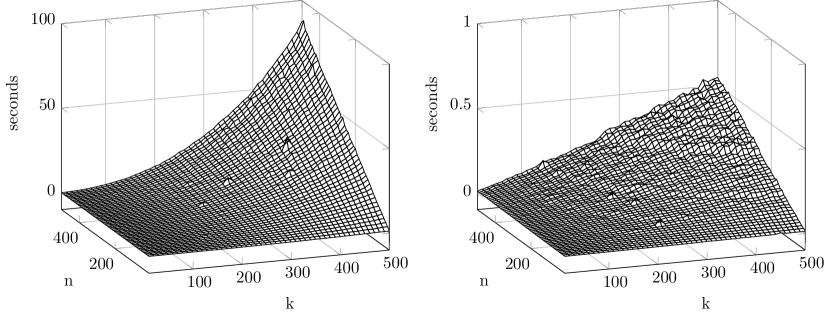
Figure 1. The run time results for Example 4 using the depth-first variant of Algorithm 1 on the left and our Algorithm 4 on the right.

These plots show a quadratic growth of Algorithm 1 in the parameter $k$ and a linear growth in the parameter $n$. For Algorithm 4 the asymptotic growth is linear in both $k$ and $n$. These observed growths coincide with the analysis that was presented in Example 4 for Algorithm 1 and on page 5 for Algorithm 4. Note that the scale of the vertical axes of both plots, displaying the run time, differs by two orders of magnitude and the highest runtime (for the $n=500$ and $k=500$ case) of Algorithm 1 is a factor 170 higher than that of Algorithm 4. As there is no difference in the data structures the difference in run time is entirely due to the different way of inspecting and extending $\mathit{working}$ and $\mathit{antichain}$.

The breadth-first variant of Algorithm 1 was unable to complete the smallest, i.e., $n=k=10$, case within the given memory limit. However, as shown in Figure 2 the run time performance of the breadth-first variant of the improved algorithm is almost equivalent to its depth-first variant.

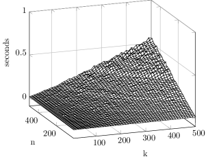
Figure 2. The run time for Example 4 using the breadth-first variant of Algorithm 4.

6.2. Experiment II: Practical Examples

The experiments that we consider are taken from two sources. First, a model of an industrial system that first exposed the performance issues in practice of a control system modelled in the Dezyne language [vBGH⁺17] . This example is of a more traditional flavour, in which the specification is an abstract description of the behaviours at the external interface of a control system, and the implementation is a detailed model that interacts with underlying services to implement the expected interface. For reasons of confidentiality, the industrial model cannot be made available.

Second, we consider several linearisability tests of concurrent data structures. These models have been taken from [Pav18], and consist of six implementations of concurrent data types that, when trace refining their specifications, are guaranteed to be linearisable. As in [WSS⁺12], we approximate trace refinement by the stronger stable failures refinement. For these models, the implementation and specification pairs are based on the same descriptions; the difference between the two is that the specification uses a simple construct to guarantee that each method of the concurrent data structure executes atomically. This significantly reduces the non-determinism and the number of transitions in the specification models.

In Table 1 the origin of each model, the number of states and transitions of each implementation and specification LTS, and whether the stable failures refinement relation holds is shown.

Table 1. The number of states and transitions in each benchmark.

Model	Ref.	states spec	trans. spec	$\bm{\sqsubseteq_{\mathsf{sfr}}}$	states impl	trans. impl
Industrial	-	24	45	True	24 551	45 447
Coarse set	[HS08]	50 488	64 729	True	55 444	145 043
Fine-grained set	[HS08]	3 720	3 305	True	5 077	9 006
Lazy set	[HS08]	3 565	3 980	True	24 496	41 431
Optimistic set	[HS08]	25 435	28 154	True	234 332	389 344
Non-blocking queue	[SHC00]	1 248	1 473	False	3 030	5 799
Treiber stack	[Tre86]	87 389	124 740	True	205 634	564 862

The run time measurements of both Algorithms 2 and 5 with both the depth-first and breadth-first variants is shown in Table 2. The run times that we report are the averages obtained from five consecutive runs.

Table 2. Run time comparison between Algorithm 2 and Algorithm 5 using depth-first (df) and breadth-first (bf) exploration.

Model	Alg. 2 df (s)	Alg. 2 bf (s)	Alg. 5 df (s)	Alg. 5 bf (s)
Industrial	1.36	296.29	0.15	0.17
Coarse set	9.15	$\dagger$	8.61	9.06
Fine-grained set	0.37	$\dagger$	0.32	0.46
Lazy set	1.19	$\dagger$	1.02	1.26
Optimistic set	16.96	$\dagger$	14.13	22.67
Non-blocking queue	0.03	0.17	0.02	0.09
Treiber stack	148.39	$\dagger$	137.52	352.59

Here, we observe that the depth-first variant of both algorithms perform similarly with a small run time advantage for Algorithm 5. However, for the breadth-first variants our algorithm is able to complete all experiments, whereas Algorithm 2 reaches the memory limit, indicated by $\dagger$, in five cases and only completes two cases successfully.

To gain more insight into the performance differences between both algorithms we repeat the experiments and report a number of performance metrics. The reported metrics are the maximum $\mathit{working}$ size and the number of $\mathit{antichain}$ membership test that fail (misses), succeed (hits) and the maximum $\mathit{antichain}$ size during the exploration. We report the maximum size instead of its size upon termination as these do not necessarily coincide, because inserting an element can evict one or more pairs in $\mathit{antichain}$. The following two tables (Tables 3 and 4) show the discussed metrics for the depth-first variant of both algorithms.

Table 3. Performance metrics for the depth-first variant of Algorithm 2.

Model	$\bm{\mathit{working}}$ max	$\bm{\mathit{antichain}}$ hits	$\bm{\mathit{antichain}}$ misses	$\bm{\mathit{antichain}}$ max
Industrial	74	36 544	43 419	43 091
Coarse set	96	93 330	58 438	55 444
Fine-grained set	60	5 786	7 575	5 077
Lazy set	61	21 184	30 771	24 496
Optimistic set	96	234 692	354 068	238 726
Non-blocking queue	52	548	672	591
Treiber stack	101	1 238 727	756 692	234 118

Table 4. Performance metrics for the depth-first variant of Algorithm 5.

Model	$\bm{\mathit{working}}$ max	$\bm{\mathit{antichain}}$ hits	$\bm{\mathit{antichain}}$ misses	$\bm{\mathit{antichain}}$ max
Industrial	69	36 369	43 090	43 091
Coarse set	96	93 330	58 438	55 444
Fine-grained set	60	5 786	7 575	5 077
Lazy set	61	21 184	30 771	24 496
Optimistic set	96	234 692	354 068	238 728
Non-blocking queue	43	520	641	634
Treiber stack	101	1 238 727	756 692	234 119

We observe in Tables 3 and 4 that only for the industrial and non-blocking queue models the performance metrics are different. An explanation for this is that because the antichain membership test is delayed (in Algorithm 2), more pairs are added to $\mathit{working}$ and these additional pairs increase the number of $\mathit{antichain}$ checks. In all other cases, the difference in run time can only be the result of the different refusal computation implementation, as the number of $\mathit{antichain}$ operations is the same.

The following two tables (Tables 5 and 6) show the obtained performance metrics for the breadth-first variants of both algorithms. In the experiments where the refinement checking terminates early, due to reaching the memory limit, we report the last observed measurements.

Table 5. Performance indicators for the breadth-first variant of Algorithm 2.

Model	$\bm{\mathit{working}}$ max	$\bm{\mathit{antichain}}$ hits	$\bm{\mathit{antichain}}$ misses	$\bm{\mathit{antichain}}$ max
Industrial	549 263	5 459 028	12 888 388	43 091
Coarse set	4 710 289	13 870	7 807 403	3 629
Fine-grained set	6 604 516	180 669	15 547 890	1 900
Lazy set	6 726 497	130 523	14 852 835	4 306
Optimistic set	6 366 524	38 649	14 238 042	4 439
Non-blocking queue	6 262	3 078	14 560	274
Treiber stack	5 829 902	76 114	8 340 606	4 811

Table 6. Performance indicators for the breadth-first variant of Algorithm 5.

Model	$\bm{\mathit{working}}$ max	$\bm{\mathit{antichain}}$ hits	$\bm{\mathit{antichain}}$ misses	$\bm{\mathit{antichain}}$ max
Industrial	2 243	36 369	43 090	43 091
Coarse set	3 411	96 167	60 332	55 444
Fine-grained set	434	7 192	9 657	5 077
Lazy set	1 748	24 340	35 192	24 496
Optimistic set	15 209	292 525	434 218	234 352
Non-blocking queue	338	3 426	4 032	2 675
Treiber stack	139 218	2 411 614	1 523 830	214 795

From these results it is clear to see that for the breadth-first variant of Algorithm 2, delaying the $\mathit{antichain}$ insertion of discovered state pairs results in an enormous overhead. The size of the $\mathit{antichain}$ remains quite small, which causes many discovered pairs to fail the antichain membership test. As each pair that fails the membership test is added to $\mathit{working}$, it causes the $\mathit{working}$ queue to grow rapidly, until it reaches the memory limit. On the other hand, for Algorithm 5 we can observe that the number of successful (and unsuccessful) $\mathit{antichain}$ membership test is quite similar to its depth-first variant. There can be some differences between these variants as the pairs are discovered in a different order. The increase of the $\mathit{working}$ size has the same reason as for ordinary breadth-first search, which depends on the out degree of the visited pairs.

To verify that the difference in performance of the depth-first variants is due to the changes of the refusal computation we have implemented another variant of Algorithm 2 with the stability check of $\mathit{impl}$ added. The run time impact of this change for both depth-first and breadth-first variants of Algorithm 2 is shown in Table 7.

Table 7. Run time results for Algorithm 2 with the stability check of $\mathit{impl}$.

Model	Alg. 2 df (s)	Alg. 2 bf (s)
Industrial	0.17	26.32
Coarse set	9.59	$\dagger$
Fine-grained set	0.36	$\dagger$
Lazy set	1.12	$\dagger$
Optimistic set	15.85	$\dagger$
Non-blocking queue	0.03	$\dagger$
Treiber stack	156.67	$\dagger$

As expected, the run time for this alternative depth-first variant closely matches the run time of the depth-first variant of the improved algorithm. The alternative breadth-first variant of Algorithm 2 is still not able to complete most experiments, but the industrial case has improved quite significantly. However, the non-blocking queue experiment now reaches the set memory limit. For this we provide the following explanation. Note that in case of a failing refinement the exploration stops when a suitable (SF-)witness has been found, which must exist as stable failures refinement does not hold. Recall that the computation of refusals for (possibly) unstable states as defined in [WSS⁺12], see Remark 22, has been implemented using a separate local search for stable states. We think that in the previous case such an SF-witness was found for an unstable state using this local search. However, in the alternative version the algorithm continues the exploration of the LTSs when encountering an unstable state (in $\mathcal{L}_{2}$), which causes the $\mathit{working}$ queue to reach the memory limit.

Finally, we repeat the same experiments while checking for failures-divergences refinement. This has only been done for Algorithm 6 as the original algorithm for failures-divergences refinement is incorrect. The run time measurements and the expected result of the failures-divergences refinement check are presented in Table 8.

Table 8. The run time results for checking failures-divergences refinement using Algorithm 6.

Model	Alg. 6 df (s)	Alg. 6 bf (s)	$\bm{\sqsubseteq_{\mathsf{fdr}}}$
Industrial	0.05	0.05	False
Coarse set	8.68	9.29	True
Fine-grained set	0.33	0.48	True
Lazy set	1.04	1.33	True
Optimistic set	14.55	23.81	True
Non-blocking queue	0.08	0.1	True
Treiber stack	140.7	363.34	True

The run time results of Table 8 show that deciding failures-divergences refinement has a similar performance to deciding stable failures.

6.3. State Space Minimisation as Preprocessing

The size of the transition systems has a major impact on the practical run time of the refinement checking algorithms we studied, as can also be seen from, e.g., Tables 1 and 2. Note that this is particularly true of the size of the specification LTS, whose normal form can be exponentially larger than the specification itself. As an alternative to the pruning achieved using antichains, reducing the size of the specification as a preprocessing step to checking for refinement may therefore be an effective tool in improving on the practical run time of these algorithms. Of course, it is desirable that the computational overhead of the reduction remains minimal. One possibility is to minimise transition systems using one of the many equivalence relations available for labelled transition systems, see, e.g. [vG93, BGR16]. When choosing such an equivalence it is important that it has the property that, apart from an appealing run time complexity, the observations, i.e., $\mathsf{weaktraces}$, $\mathsf{failures}$ and $\mathsf{divergences}$, that are extracted from equivalent states are the same.

Strong bisimilarity is known to preserve the $\mathsf{weaktraces}$, $\mathsf{failures}$ and $\mathsf{divergences}$ observations of equivalent states. However, a more substantial state space reduction can often be achieved by considering equivalences that treat the special action $\tau$ as invisible, as the given LTSs often contain $\tau$-transitions. In [Ros10], Roscoe suggests to use a variant of weak bisimulation, viz., divergence respecting weak bisimulation, to minimise a transition system. For divergence respecting weak bisimulation it is known that it is a suitable abstraction; see the following theorem [Ros10, Theorem 9.2].

Theorem 37.

Let $\mathcal{L}=(\mathit{S},\iota,\rightarrow)$ be an LTS. For two states $s,t\in\mathit{S}$ that are divergence respecting weak bisimilar it holds that $\mathsf{weaktraces}(s)=\mathsf{weaktraces}(t)$, $\mathsf{divergences}(s)=\mathsf{divergences}(t)$, $\mathsf{failures}(s)=\mathsf{failures}(t)$. Hence, also $\mathsf{failures}_{\bot}(s)=\mathsf{failures}_{\bot}(t)$.

From a computational point of view, however, (divergence respecting) weak bisimulation is not particularly promising. For instance, the best known algorithm [RT08] for computing weak bisimulation has a worst-case time complexity of $\mathcal{O}(m\cdot n)$, where $n$ is the number of states and $m$ the number of transitions. Such run time complexities are non-neglible and may result in an undesirable overhead.

In practice, divergence-respecting weak bisimulation often coincides with divergence preserving branching bisimulation and it has the far more appealing worst-case run time complexity of $\mathcal{O}(m\cdot\log n)$ [JGKW20], which is equivalent to the run time complexity of computing strong bisimulation [PT87]. Divergence-preserving branching bisimulation is stronger than divergence respecting weak bisimulation, i.e., two states that are divergence-preserving branching bisimilar are also divergence respecting weak bisimilar. Divergence-preserving branching bisimilarity is, by Theorem 37, therefore a suitable abstraction.

The algorithm that decides divergence-preserving branching bisimulation equivalence between two states can also be adapted to a minimisation procedure with the same $\mathcal{O}(m\cdot\log n)$ time complexity. We have made the preprocessing step of minimisation modulo divergence-preserving branching bisimulation available as an option in our tool. In Table 9 the number of states and transitions of each model of Section 6.2, after minimisation modulo divergence-preserving branching bisimulation, and whether the specification and implementation LTSs are divergence-preserving branching bisimilar is shown.

Table 9. The number of states and transitions after diverging preserving branching bisimulation minimisation and whether the LTSs are equivalent in divergence-preserving branching bisimulation semantics denoted by $\leftrightarroweq_{db}$.

Model	states spec	trans. spec	$\bm{\leftrightarroweq_{db}}$	states impl	trans. impl
Industrial	24	45	False	4 626	14 380
Coarse set	1 089	3 618	True	1 089	3 618
Fine-grained set	92	210	True	92	210
Lazy set	92	210	True	92	210
Optimistic set	170	410	True	170	410
Non-blocking queue	119	274	False	163	378
Treiber stack	7 988	26 070	True	7 988	26 070

Observe that for most of the models, the minimised implementation and specification LTSs are of equal size; indeed, in those cases the implementation and specification are divergence-preserving branching bisimulation equivalent, so no further stable failures refinement check would be needed.

One option would therefore be to apply the minimisation to both implementation and specification LTSs. This approach turns out to be beneficial for the Treiber stack example, obtaining a run time of 3 seconds to determine stable failures refinement. The approach is not beneficial for the other examples. Moreover, minimising the implementation might even be less effective in case the refinement relation between specification and implementation does not hold, in which case the refinement check will probably quickly determine this fact.

We therefore measure the effect of using minimised specifications, but unmodified implementations. The run time measurements of checking stable failures refinement using Algorithms 2 and 5 using the minimised specification LTS is shown in Table 10. The time that it takes to compute the divergence-preserving branching bisimulation minimisation is presented in the last column and the other measurements are the run time of the algorithm including preprocessing.

Table 10. Run time comparison between the original algorithm (Algorithm 2) and the improved algorithm (Algorithm 5) using depth-first (df) and breadth-first (bf) exploration where the specification is reduced modulo divergence-preserving branching bisimulation.

Model	Alg. 2 df (s)	Alg. 2 bf (s)	Alg. 5 df (s)	Alg. 5 bf (s)	Reduction (s)
Industrial	1.38	293.1	0.16	0.17	0.01
Coarse set	0.74	$\dagger$	0.69	0.69	0.10
Fine-grained set	0.04	$\dagger$	0.04	0.04	0.01
Lazy set	0.21	$\dagger$	0.15	0.15	0.01
Optimistic set	2.52	$\dagger$	1.59	1.57	0.04
Non-blocking queue	0.02	0.04	0.02	0.02	0.01
Treiber stack	8.19	$\dagger$	6.61	11.71	0.24

Comparing these results with Table 2 shows that reducing the specification modulo divergence-preserving branching bisimulation can indeed substantially improve the performance of the antichain-based algorithms. In particular, it never degrades the performance of our algorithms as the preprocessing time is negligible. For failures-divergences refinement the results, using Algorithm 6, are similar, as is shown in Table 11.

Table 11. The run time results for checking failures-divergences refinement using Algorithm 6 where the specification is reduced module divergence-preserving branching bisimulation.

Model	Alg. 6 df (s)	Alg. 6 bf (s)
Industrial	0.05	0.06
Coarse set	0.75	0.7
Fine-grained set	0.04	0.04
Lazy set	0.15	0.15
Optimistic set	1.61	1.7
Non-blocking queue	0.02	0.02
Treiber stack	6.76	12.13

7. Conclusion

Our study of the antichain-based algorithms for deciding trace refinement, stable failures refinement and failures-divergences refinement presented in [WSS⁺12] revealed that the failures-divergences refinement algorithm is incorrect. All three algorithms perform suboptimally when implemented using a depth-first search strategy and poorly when implemented using a breadth-first search strategy. Furthermore, all three algorithms violate the claimed antichain property. We propose alternative algorithms for which we have shown correctness and which utilise proper antichains. Our experiments indicate significant performance improvements for deciding trace refinement, stable failures refinement and a performance of deciding failures-divergences refinement that is comparable to deciding stable failures refinement. We also show that preprocessing using divergence-preserving branching bisimulation offers substantial performance benefits. The implementation of our algorithms is available in the open source toolset mCRL2 [BGK⁺19] and is currently used as the backbone in the commercial F-MDE toolset Dezyne; see also [vBGH⁺17].

Appendix A Proof of Lemma 5

See 5

Proof A.1.

We use induction on the length of sequences in $\mathit{Act}^{*}$ to prove the statement.

Base case. First, $\iota^{\prime}\xrightarrow{\epsilon}\!\!\!\!\!\rightarrow^{\prime}U$ iff $U=\iota^{\prime}$ by definition. The state $\iota^{\prime}$ is equal to $\{s\mid\iota\overset{\epsilon}{\Longrightarrow}s\}$ as defined in the normalisation. Hence, for every state $s\in[\![\iota^{\prime}\mkern 1.0mu]\!]_{\mathcal{L}}$ we have $\iota\overset{\epsilon}{\Longrightarrow}s$.

Inductive case. Pick any sequence $\rho\in\mathit{Act}^{*}$ of length $i$ and suppose that the statement holds for all sequences in $\mathit{Act}^{*}$ of length $i$. Take an arbitrary state $V\in\mathit{S}^{\prime}$ and action $a\in\mathit{Act}$ such that $\iota^{\prime}\xrightarrow{\rho\,a}\!\!\!\!\!\rightarrow^{\prime}V$. Then there is a state $U\in\mathit{S}^{\prime}$ such that $\iota^{\prime}\xrightarrow{\rho}\!\!\!\!\!\rightarrow^{\prime}U$ and $U\xrightarrow{a}\!\!\!\!\!\!\rightarrow^{\prime}V$. By definition of normalisation there is a transition $U\xrightarrow{a}\!\!\!\!\!\!\rightarrow^{\prime}V$ if and only if $V=\{t\in\mathit{S}\mid\exists s\in U:s\overset{a}{\Longrightarrow}t\}$. So for all states $t\in[\![V\mkern 1.0mu]\!]_{\mathcal{L}}$ there is a state $s\in[\![U\mkern 1.0mu]\!]_{\mathcal{L}}$ such that $s\overset{a}{\Longrightarrow}t$. By the induction hypothesis it holds that for all $s\in[\![U\mkern 1.0mu]\!]_{\mathcal{L}}$ there is a weak transition $\iota\overset{\rho}{\Longrightarrow}s$. But then we may conclude that $\iota\overset{\rho\,a}{\Longrightarrow}t$ for all $t\in[\![V\mkern 1.0mu]\!]_{\mathcal{L}}$.

Appendix B Proof of Lemma 6

See 6

Proof B.1.

We proceed using an induction on the length of sequences in $\mathit{Act}^{*}$.

Base case. Let $s\in\mathit{S}$ and suppose $\iota\overset{\epsilon}{\Longrightarrow}s$. Then $s\in[\![\iota^{\prime}\mkern 1.0mu]\!]_{\mathcal{L}}$, since $\iota^{\prime}$ is defined as $\{s\in\mathit{S}\mid\iota\overset{\epsilon}{\Longrightarrow}s\}$. Moreover, we trivially have $\iota^{\prime}\xrightarrow{\epsilon}\!\!\!\!\!\rightarrow^{\prime}\iota^{\prime}$.

Inductive step. Pick any sequence $\rho\in\mathit{Act}^{*}$ of length $i$ and suppose that the statement holds for all sequences in $\mathit{Act}^{*}$ of length $i$. Take an arbitrary state $t\in\mathit{S}$ and action $a\in\mathit{Act}$ such that $\iota\overset{\rho\,a}{\Longrightarrow}t$. Then there is a state $s\in\mathit{S}$ such that $\iota\overset{\rho}{\Longrightarrow}s$ and $s\overset{a}{\Longrightarrow}t$. Fix such a state $s\in\mathit{S}$. From the induction hypothesis it then follows that there is a state $U\in\mathit{S}^{\prime}$ such that $s\in[\![U\mkern 1.0mu]\!]_{\mathcal{L}}$ and $\iota^{\prime}\xrightarrow{\rho}\!\!\!\!\!\rightarrow^{\prime}U$. Fix this state $U\in\mathit{S}^{\prime}$. Let $V$ be equal to $\{t\in\mathit{S}\mid\exists u\in U:u\overset{a}{\Longrightarrow}t\}$; then by definition, $U\xrightarrow{a}\!\!\!\!\!\!\rightarrow^{\prime}V$. It follows that $\iota^{\prime}\xrightarrow{\rho\,a}\!\!\!\!\!\rightarrow^{\prime}V$. Finally, $t\in[\![V\mkern 1.0mu]\!]_{\mathcal{L}}$ follows from $s\overset{a}{\Longrightarrow}t$ and $s\in[\![U\mkern 1.0mu]\!]_{\mathcal{L}}$.

Appendix C Proof of Lemma 7

See 7

Proof C.1.

• We use induction on the length of the sequences in $\mathit{Act}^{*}$.

  Base case. The implication holds vacuously since $\epsilon\in\mathsf{weaktraces}(\mathcal{L})$.

  Inductive step. Pick a sequence $\rho\in\mathit{Act}^{*}$ of length $i$ and suppose that the implication holds for all sequences of length $i$. Assume an arbitrary action $a\in\mathit{Act}$ such that $\rho\,a\notin\mathsf{weaktraces}(\mathcal{L})$. From $\rho\,a\notin\mathsf{weaktraces}(\mathcal{L})$ it follows that there is no state $t\in\mathit{S}$ such that $\iota\overset{\rho\,a}{\Longrightarrow}t$. We distinguish two cases:

  • Case $\rho\notin\mathsf{weaktraces}(\mathcal{L})$. From the induction hypothesis we obtain $\iota^{\prime}\xrightarrow{\rho}\!\!\!\!\!\rightarrow^{\prime}\emptyset$ and $\emptyset\xrightarrow{a}\!\!\!\!\!\!\rightarrow^{\prime}\emptyset$ by definition. We may therefore also conclude $\iota^{\prime}\xrightarrow{\rho\,a}\!\!\!\!\!\rightarrow^{\prime}\emptyset$.

  • Case $\rho\in\mathsf{weaktraces}(\mathcal{L})$. Then there is a state $s\in\mathit{S}$ such that $\iota\overset{\rho}{\Longrightarrow}s$. Since $\mathcal{L}^{\prime}$ is deterministic there is a unique state $U\in\mathit{S}^{\prime}$ such that both $s\in[\![U\mkern 1.0mu]\!]_{\mathcal{L}}$ and $\iota^{\prime}\xrightarrow{\rho}\!\!\!\!\!\rightarrow^{\prime}U$ by Lemmas 6 and 1. For all states $u\in\mathit{S}$ satisfying $\iota\overset{\rho}{\Longrightarrow}u$ (which exist as $\rho\in\mathsf{weaktraces}(\mathcal{L})$) there cannot be a state $t\in\mathit{S}$ such that $u\overset{a}{\Longrightarrow}t$ by the observation that $\rho\,a\notin\mathsf{weaktraces}(\mathcal{L})$. Therefore, $U\xrightarrow{a}\!\!\!\!\!\!\rightarrow^{\prime}\emptyset$ and thus also $\iota^{\prime}\xrightarrow{\rho\,a}\!\!\!\!\!\rightarrow^{\prime}\emptyset$.

• Suppose $\iota^{\prime}\xrightarrow{\rho}\!\!\!\!\!\rightarrow^{\prime}\emptyset$. Towards a contradiction, assume that $\rho\in\mathsf{weaktraces}(\mathcal{L})$. Then there is a state $s\in\mathit{S}$ such that $\iota\overset{\rho}{\Longrightarrow}s$. By Lemma 6, there must be some $U\in\mathit{S}^{\prime}$ such that $s\in[\![U\mkern 1.0mu]\!]_{\mathcal{L}}$ and $\iota^{\prime}\xrightarrow{\rho}\!\!\!\!\!\rightarrow^{\prime}U$. Since $\mathcal{L}^{\prime}$ is deterministic, by Lemma 1, we obtain that this state $U$ must be such that $U=\emptyset$.

Appendix D Proof of Lemma 15

See 15

Proof D.1.

Proof by induction on the length of sequences that are not divergences, or minimal divergences.

Base case. The empty trace $\epsilon$ satisfies $\epsilon\notin\mathsf{divergences}(\mathcal{L})$ or $\epsilon\in\mathsf{divergences}_{\mathsf{min}}(\mathcal{L})$ by definition. Hence, we must show that for all states $s\in\mathit{S}$ satisfying $\iota\overset{\epsilon}{\Longrightarrow}s$ there is a state $U\in\mathit{S}^{\prime}$ such that $s\in[\![U\mkern 1.0mu]\!]_{\mathcal{L}}$ and $\iota^{\prime}\xrightarrow{\epsilon}\!\!\!\!\!\rightarrow^{\prime}U$. We know that if $\iota\overset{\epsilon}{\Longrightarrow}s$ then $s\in[\![\iota^{\prime}\mkern 1.0mu]\!]_{\mathcal{L}}$, because $\iota^{\prime}$ is defined as $\{s\in\mathit{S}\mid\iota\overset{\epsilon}{\Longrightarrow}s\}$ in the normalisation. Finally, we also know that $\iota^{\prime}\xrightarrow{\epsilon}\!\!\!\!\!\rightarrow^{\prime}\iota^{\prime}$.

Inductive step. Suppose that the statement holds for all sequences of length $i$ that are either not divergences or minimal divergences of $\mathcal{L}$. Pick a sequence $\rho\in\mathit{Act}^{*}$ of length $i$, an arbitrary state $t\in\mathit{S}$ and action $a\in\mathit{Act}$ such that $\iota\overset{\rho\,a}{\Longrightarrow}t$ and $\rho\,a\notin\mathsf{divergences}(\mathcal{L})$ or $\rho\,a\in\mathsf{divergences}_{\mathsf{min}}(\mathcal{L})$. Note that whenever $\rho\,a\notin\mathsf{divergences}(\mathcal{L})$ or $\rho\,a\in\mathsf{divergences}_{\mathsf{min}}(\mathcal{L})$ then $\rho\notin\mathsf{divergences}(\mathcal{L})$. From $\iota\overset{\rho\,a}{\Longrightarrow}t$ it follows that there is a state $s\in\mathit{S}$ such that $\iota\overset{\rho}{\Longrightarrow}s$ and $s\overset{a}{\Longrightarrow}t$. By our induction hypothesis it then follows that there is a state $U\in\mathit{S}^{\prime}$ such that $s\in[\![U\mkern 1.0mu]\!]_{\mathcal{L}}$ and $\iota^{\prime}\xrightarrow{\rho}\!\!\!\!\!\rightarrow^{\prime}U$. For all states $u\in[\![U\mkern 1.0mu]\!]_{\mathcal{L}}$ it holds that $\iota\overset{\rho}{\Longrightarrow}u$ by Lemma 14, so by definition of divergences it must be that $u\raisebox{1.0pt}{$\Uparrow$}$ does not hold and hence $[\![U\mkern 1.0mu]\!]_{\mathcal{L}}\raisebox{1.0pt}{$\Uparrow$}$ does not hold. Let $V$ be equal to $\{v\in\mathit{S}\mid\exists u\in U:u\overset{a}{\Longrightarrow}v\}$ such that $U\xrightarrow{a}\!\!\!\!\!\!\rightarrow^{\prime}V$ by definition of the normalisation. It follows that $\iota^{\prime}\xrightarrow{\rho\,a}\!\!\!\!\!\rightarrow^{\prime}V$. Finally, $t\in[\![V\mkern 1.0mu]\!]_{\mathcal{L}}$ follows from $s\overset{a}{\Longrightarrow}t$ and $s\in[\![U\mkern 1.0mu]\!]_{\mathcal{L}}$.

Appendix E Proof of Lemma 16

See 16

Proof E.1.

Let $\rho\in\mathit{Act}^{*}$ and $U\in\mathit{S}^{\prime}$ be such that $\iota^{\prime}\xrightarrow{\rho}\!\!\!\!\!\rightarrow^{\prime}U$ and not $[\![U\mkern 1.0mu]\!]_{\mathcal{L}}\raisebox{1.0pt}{$\Uparrow$}$. Towards a contradiction, assume that $\rho\in\mathsf{divergences}(\mathcal{L})$. We distinguish two cases:

• $\rho\in\mathsf{divergences}_{\mathsf{min}}(\mathcal{L})$. Let $t\in\mathit{S}$ be such that $\iota\overset{\rho}{\Longrightarrow}t$ and $t\raisebox{1.0pt}{$\Uparrow$}$. Note that due to the determinism of $\mathsf{norm}_{\mathsf{fdr}}(\mathcal{L})$ and Lemma 15, for all $s\in\mathit{S}$ such that $\iota\overset{\rho}{\Longrightarrow}s$, we have $s\in U$. Hence also $t\in U$. But $t\raisebox{1.0pt}{$\Uparrow$}$ then implies $[\![U\mkern 1.0mu]\!]_{\mathcal{L}}\raisebox{1.0pt}{$\Uparrow$}$. Contradiction.

• $\rho\notin\mathsf{divergences}_{\mathsf{min}}(\mathcal{L})$. Then $\rho=\rho^{\prime}\rho^{\prime\prime}$ for some $\rho^{\prime}\in\mathsf{divergences}_{\mathsf{min}}(\mathcal{L})$. Let $t\in\mathit{S}$ be such that $\iota\overset{\rho^{\prime}}{\Longrightarrow}t$ and $t\raisebox{1.0pt}{$\Uparrow$}$. Then, by Lemma 15, there must be some $V\in\mathit{S}^{\prime}$ such that $\iota^{\prime}\xrightarrow{\rho^{\prime}}\!\!\!\!\!\rightarrow^{\prime}V$ and $t\in V$. Let $V$ be such. Since $t\raisebox{1.0pt}{$\Uparrow$}$ and $t\in V$, $V$ has no outgoing transitions in $\mathsf{norm}_{\mathsf{fdr}}(\mathcal{L})$. In particular, we cannot have $V\xrightarrow{\rho^{\prime\prime}}\!\!\!\!\!\rightarrow^{\prime}U$, and because $\mathsf{norm}_{\mathsf{fdr}}(\mathcal{L})$ is deterministic, we also cannot have $\iota^{\prime}\xrightarrow{\rho}\!\!\!\!\!\rightarrow^{\prime}U$. Contradiction.

Appendix F Proof of Lemma 17

See 17

Proof F.1.

• Proof by induction on the length of sequences in $\mathit{Act}^{*}$.

  Base case. The implication holds vacuously since $\epsilon\in\mathsf{weaktraces}(\mathcal{L})$.

  Inductive step. Suppose that the statement holds for all sequences $\mathit{Act}^{*}$ of length $i$. Pick a sequence $\rho\in\mathit{Act}^{*}$ of length $i$. Take an arbitrary action $a\in\mathit{Act}$ such that $\rho\,a\notin(\mathsf{divergences}(\mathcal{L})\cup\mathsf{weaktraces}(\mathcal{L}))$. From $\rho\,a\notin\mathsf{weaktraces}(\mathcal{L})$ it follows that there is no state $t\in\mathit{S}$ such that $\iota\overset{\rho\,a}{\Longrightarrow}t$. From $\rho\,a\notin\mathsf{divergences}(\mathcal{L})$ it follows that $\rho\notin\mathsf{divergences}(\mathcal{L})$. Now, there are two cases to distinguish:

  • Case $\rho\notin\mathsf{weaktraces}(\mathcal{L})$. From the induction hypothesis we obtain $\iota^{\prime}\xrightarrow{\rho}\!\!\!\!\!\rightarrow^{\prime}\emptyset$ and $\emptyset\xrightarrow{a}\!\!\!\!\!\!\rightarrow^{\prime}\emptyset$ by definition. Thus $\iota^{\prime}\xrightarrow{\rho\,a}\!\!\!\!\!\rightarrow^{\prime}\emptyset$.

  • Case $\rho\in\mathsf{weaktraces}(\mathcal{L})$. There is a state $s\in\mathit{S}$ such that $\iota\overset{\rho}{\Longrightarrow}s$. Since $\mathcal{L}^{\prime}$ is deterministic there is a unique state $U\in\mathit{S}^{\prime}$ such that $s\in[\![U\mkern 1.0mu]\!]_{\mathcal{L}}$ and $\iota^{\prime}\xrightarrow{\rho}\!\!\!\!\!\rightarrow^{\prime}U$ by Lemma 15 and 1. We may furthermore conclude that $[\![U\mkern 1.0mu]\!]_{\mathcal{L}}\raisebox{1.0pt}{$\Uparrow$}$ does not hold. Because $\rho\,a\notin\mathsf{weaktraces}(\mathcal{L})$, no state $u\in\mathit{S}$ for which $\iota\overset{\rho}{\Longrightarrow}u$ satisfies $u\overset{a}{\Longrightarrow}t$, for any state $t$. Therefore, by definition, $U\xrightarrow{a}\!\!\!\!\!\!\rightarrow^{\prime}\emptyset$, and thus $\iota^{\prime}\xrightarrow{\rho\,a}\!\!\!\!\!\rightarrow^{\prime}\emptyset$.

• Suppose $\iota^{\prime}\xrightarrow{\rho}\!\!\!\!\!\rightarrow^{\prime}\emptyset$. From the observation that $[\![\emptyset\mkern 1.0mu]\!]_{\mathcal{L}}\raisebox{1.0pt}{$\Uparrow$}$ does not hold and Lemma 16 it follows that $\rho\notin\mathsf{divergences}(\mathcal{L})$. Towards a contradiction, assume that $\rho\in\mathsf{weaktraces}(\mathcal{L})$. Then there is a state $s\in\mathit{S}$ such that $\iota\overset{\rho}{\Longrightarrow}s$. By Lemma 17, there must be some $U\in\mathit{S}^{\prime}$ such that $s\in[\![U\mkern 1.0mu]\!]_{\mathcal{L}}$ and $\iota^{\prime}\xrightarrow{\rho}\!\!\!\!\!\rightarrow^{\prime}U$. Since $\mathcal{L}^{\prime}$ is deterministic, by Lemma 1, we obtain that this state $U$ must be such that $U=\emptyset$. Contradiction.

References

- [ACH+10] P. A. Abdulla, Y.-F. Chen, L. Holík, R. Mayr, and T. Vojnar. When simulation meets antichains. In J. Esparza and R. Majumdar, editors, TACAS 2010, volume 6015 of LNCS, pages 158–174. Springer, 2010.
- [BGK+19] O. Bunte, J. F. Groote, J. J. A. Keiren, M. Laveaux, T. Neele, E. P. de Vink, J. W. Wesselink, A. Wijs, and T. A. C. Willemse. The mCRL2 toolset for analysing concurrent systems - improvements in expressivity and usability. In T. Vojnar and L. Zhang, editors, TACAS 2019, volume 11428 of LNCS, pages 21–39. Springer, 2019.
- [BGR16] A. Boulgakov, T. Gibson-Robinson, and A. W. Roscoe. Computing maximal weak and other bisimulations. Formal Asp. Comput., 28(3):381–407, 2016.
- [BKO87] J. A. Bergstra, J. W. Klop, and E.-R. Olderog. Failures without chaos: a new process semantics for fair abstraction. In M. Wirsing, editor, IFIP TC 2/WG 2.2 1986, pages 77–104. North-Holland, 1987.
- [BR84] S. D. Brookes and A. W. Roscoe. An improved failures model for communicating processes. In S. D. Brookes, A. W. Roscoe, and Glynn Winskel, editors, Seminar on Concurrency 1984, volume 197 of LNCS, pages 281–305. Springer, 1984.
- [DR10] L. Doyen and J.-F. Raskin. Antichain algorithms for finite automata. In TACAS, volume 6015 of Lecture Notes in Computer Science, pages 2–22. Springer, 2010.
- [GABR14] T. Gibson-Robinson, P. J. Armstrong, A. Boulgakov, and A. W. Roscoe. FDR3 - A modern refinement checker for CSP. In E. Ábrahám and K. Havelund, editors, TACAS 2014, volume 8413 of LNCS, pages 187–201. Springer, 2014.
- [GABR16] T. Gibson-Robinson, P. J. Armstrong, A. Boulgakov, and A. W. Roscoe. FDR3: a parallel refinement checker for CSP. STTT, 18(2):149–167, 2016.
- [GB16] A. O. Gomes and A. Butterfield. Modelling the haemodialysis machine with circus. In M. J. Butler, K.-D. Schewe, A. Mashkoor, and M. Biró, editors, ABZ 2016, volume 9675 of LNCS, pages 409–424. Springer, 2016.
- [GBC+17] T. Gibson-Robinson, G. H. Broadfoot, G. Carvalho, P. J. Hopcroft, G. Lowe, S. Nogueira, C. O’Halloran, and A. Sampaio. FDR: from theory to industrial application. In Concurrency, Security, and Puzzles, volume 10160 of Lecture Notes in Computer Science, pages 65–87. Springer, 2017.
- [Hoa85] C. A. R. Hoare. Communicating Sequential Processes. Prentice-Hall, 1985.
- [HS08] M. Herlihy and N. Shavit. The art of multiprocessor programming. Morgan Kaufmann, 2008.
- [JGKW20] D. N. Jansen, J. Friso Groote, J. J. A. Keiren, and A. Wijs. An O(m log n) algorithm for branching bisimilarity on labelled transition systems. In TACAS (2), volume 12079 of Lecture Notes in Computer Science, pages 3–20. Springer, 2020.
- [KS90] P. C. Kanellakis and S. A. Smolka. CCS expressions, finite state processes, and three problems of equivalence. Inf. Comput., 86(1):43–68, 1990.
- [Lav19] M. Laveaux. Downloadable sources and benchmarks for the experimental validation. 2019. https://doi.org/10.5281/zenodo.3449420.
- [LGW19] M. Laveaux, J. F. Groote, and T. A. C. Willemse. Correct and efficient antichain algorithms for refinement checking. In FORTE, volume 11535 of Lecture Notes in Computer Science, pages 185–203. Springer, 2019.
- [Pav18] R. Paval. Modeling and verifying concurrent data structures. Master’s thesis, Eindhoven University of Technology, 2018. https://research.tue.nl/files/93882157/Thesis_Roxana_Paval.pdf.
- [PT87] Robert Paige and Robert Endre Tarjan. Three partition refinement algorithms. SIAM J. Comput., 16(6):973–989, 1987.
- [Ros94] A. W. Roscoe. Model-checking CSP. In A. W. Roscoe, editor, A Classical Mind: essays in Honour of C. A. R. Hoare, chapter 21, pages 353–378. Prentice Hall International (UK) Ltd., 1994.
- [Ros10] A. W. Roscoe. Understanding Concurrent Systems. Texts in Computer Science. Springer, 2010.
- [RT08] F. Ranzato and F. Tapparo. Generalizing the paige-tarjan algorithm by abstract interpretation. Inf. Comput., 206(5):620–651, 2008.
- [SHC00] C.-H. Shann, T.-L. Huang, and C. Chen. A practical nonblocking queue algorithm using compare-and-swap. In ICPADS 2000, pages 470–475. IEEE Computer Society, 2000.
- [Tre86] R. K. Treiber. Systems programming: Coping with parallelism. International Business Machines Incorporated, Thomas J. Watson Research, 1986.
- [vBGH+17] R. van Beusekom, J. F. Groote, P. F. Hoogendijk, R. Howe, J. W. Wesselink, R. Wieringa, and T. A. C. Willemse. Formalising the Dezyne modelling language in mCRL2. In L. Petrucci, C. Seceleanu, and A. Cavalcanti, editors, FMICS-AVoCS 2017, volume 10471 of LNCS, pages 217–233. Springer, 2017.
- [vG93] R. J. van Glabbeek. The linear time - branching time spectrum II. In E. Best, editor, CONCUR 1993, volume 715 of LNCS, pages 66–81. Springer, 1993.
- [vG17] R. J. van Glabbeek. A branching time model of CSP. In T. Gibson-Robinson, P. J. Hopcroft, and R. Lazic, editors, Concurrency, Security, and Puzzles - Essays Dedicated to Andrew William Roscoe on the Occasion of His 60th Birthday, volume 10160 of LNCS, pages 272–293. Springer, 2017.
- [vG19] R. J. van Glabbeek, 2019. Personal Communication, 7 January 2019.
- [vGLT09] R. J. van Glabbeek, B. Luttik, and N. Trc̆ka. Branching bisimilarity with explicit divergence. Fundam. Inform., 93(4):371–392, 2009.
- [vGW96] R. J. van Glabbeek and W. P. Weijland. Branching time and abstraction in bisimulation semantics. J. ACM, 43(3):555–600, 1996.
- [WDHR06] M. De Wulf, L. Doyen, T. A. Henzinger, and J.-F. Raskin. Antichains: A new algorithm for checking universality of finite automata. In Thomas Ball and Robert B. Jones, editors, Computer Aided Verification, 18th International Conference, CAV 2006, Seattle, WA, USA, August 17-20, 2006, Proceedings, volume 4144 of Lecture Notes in Computer Science, pages 17–30. Springer, 2006.
- [WSS+12] T. Wang, S. Song, J. Sun, Y. Liu, J. S. Dong, X. Wang, and S. Li. More anti-chain based refinement checking. In T. Aoki and K. Taguchi, editors, ICFEM, volume 7635 of LNCS, pages 364–380. Springer, 2012.