The category of cellular resolutions
Abstract
Cellular resolutions are a well-studied topic on the level of single resolutions and certain specific families of cellular resolutions. One question coming out of the work on families is to understand the structure of cellular resolutions more generally. We give a starting point to understanding higher level structures by defining the category of cellular resolutions. In this paper we study the properties of this category. The main results are in lifting homotopy colimits from topology and Morse theory on cellular resolution being compatible with the category.
1 Introduction
Cellular resolutions were first introduced by Bayer and Sturmfels in [3] in order to study monomial modules. Earlier work of Bayer, Peeva and Sturmfels [2] introduced the concept for simplicial cases. Cellular resolutions have turned out to be a strong tool for resolving monomial modules and they are now a standard tool in combinatorial commutative algebra, and thus covered in the book by Miller and Sturmfels [16], for example. The definition of cellular resolutions with cell complexes brings in topology and also gives them a combinatorial nature, so we know very well how to compute them. A lot of the literature on cellular resolutions either cover a particular type of monomial ideals, for example Dochtermann and Mohammadi construct cellular resolutions from mapping cones in [8], or are very involved with minimality of the resolution. It is known that every monomial module has a non-minimal cellular resolution, but in [20] Velasco showed that not all of them have a minimal cellular resolution.
Despite all the known facts about cellular resolutions, they have not been studied as a class of objects. There has been a discussion on the general structure of cellular resolutions, see for example [8] for open question on ”moduli space” for a family of cellular resolutions, and even these cases are often focused on the structure of the particular family of cellular resolutions. A natural question would be to ask how do cellular resolutions behave in a more category-theoretic setting. This approach is also supported by the existing conversation on higher structrures on cellular resolutions, and that category theory is a fundamental tool in studying these in other fields like algebraic geometry and representation stability. In this paper, we define the category of cellular resolutions and study some of its properties. This is not only interesting in its own right, but also can help us to understand cellular resolutions in general. Studying subcategories opens up a novel way to study specific types of cellular resolutions, and category theoretic constructions give us new ways to build cellular resolutions from the existing ones.
We start by generalizing the definition of cellular resolutions to cases where the cell complexes may not be connected, and then continue by defining what a map between two cellular resolutions is. For this we need the concept of compatible cellular and chain map which says that “they both do the same thing”. Our main result, in Definition 3.20 and Theorem 3.21, is the definition of the category of cellular resolutions, CellRes, and that it does indeed form a category.
Theorem.
CellRes with objects being cellular resolutions and their direct sums, and morphisms being pairs of compatible chain maps and cellular maps, is a well-defined category.
In Sections 4, 5, 6 and 7 we study the common constructions in CellRes, and note other worthwhile observations. These include mapping cones and cylinders, (co)products and (co)limits. Throughout these sections, we see the repeating pattern of well-behaved constructions for cellular resolutions if topological and chain complex constructions are essentially the same. Otherwise, they may not even exist in the category CellRes in general.
In Section 8 we turn our attention to homotopy colimits. They are a well known construction in topology, and we show that the explicit construction lifts to CellRes.
Theorem.
Homotopy colimits lift from topology to cellular resolutions
In particular, this gives us a good way to construct explicit cellular resolutions from known ones.
In the final Section 9, we focus on discrete Morse theory on cellular resolutions. The interest in minimality has also motivated the application of discrete Morse theory to cellular resolutions in earlier work, and one example is [13] where it is shown how to make a resolution closer to a minimal one. We show that the algebraic Morse theory and the discrete Morse theory for cellular resolutions work well together. Our main result from this section is the following:
Theorem.
Let be a cellular resolution with a cell complex , and let be a Morse matching on them.
Let be the chain map from to , and let be the cellular strong deformation retract of coming from the Morse theory.
Then the pair formed of the Morse maps is a morphisms in CellRes.
This result shows that Morse maps are well behaved with respect to algebra and topology on cellular resolutions. Furthermore, the results on Morse theory gives a basis for simple homotopy theory for cellular resolutions. As the last result we define a simple homotopy equivalence of cellular resolutions.
This work serves as stepping stone for further questions of categorical nature. In particular, it opens up cellular resolutions to representation stability in the sense of Sam and Snowden [17], and this was one of our main motivations for writing this paper. We would like to apply the representation stability results presented in the work of Sam and Snowden to CellRes, and for this we need to have the cellular resolutions as a category. In particular, this includes the results on noetherianity and finite generation of representations, for example Theorem 1.1.3 of [17], applied to representations of cellular resolutions. The full details of the representation stability aspects of cellular resolutions will be made available shortly in our paper that is currently in progress.
Acknowledgements
I would like to thank Alexander Engström for many helpful discussions and guidance.
2 Background
In this section we review the existing tools and definitions that we will need later.
2.1 Category theory
There are many good references for introductory category theory, and our main references are [4], [5] and [14].
One of the most important definitions that we need from category theory is the definition of a (locally small) category itself.
Definition 2.1.
A (locally small) category consists of a class of objects and a set of morphisms for each pair of objects . For any triple we have composition map of the morphisms , with the image of the pair denoted by . The category must satisfy the following two conditions:
-
1.
For any object there exists an identity morphism such that and .
-
2.
Composition of morphisms is associative, that is for all and .
We also require that the morphism sets and are disjoint unless and .
We say that a category is small if the objects and morphisms form a set.
Common examples of categories include Set: where the objects are sets and the morphisms are set maps, Top: objects are topological spaces and morphisms are continuous maps, and : objects are modules over the ring and morphisms are module homomorphims.
Subcategories of the category of cellular resolutions are briefly discussed in the Section 3.3.1, for that we have the defintion of a subcategory below.
Definition 2.2.
A subcategory of is a category where and morphisms of such that the source, target, and composition are the same as in . A subcategory of is full if for any pair .
Next we define some common category theory concepts that are needed to study the basic properties of the category of cellular resolutions.
Definition 2.3.
An object is said to be an initial object if for all objects there is a single morphism . Similarly we say that is a final object if there is a unique morphism for all . If the initial and final objects exists, they are unique up to an isomorphism.
The product and coproduct constructions play a significant role for the properties that the category of cellular resolutions has and thus we state them here. For examples of product and coproduct we have them for the categories Top and in Section 2.2.
Definition 2.4.
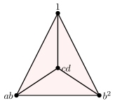
A product of two objects in the category is an object such that there exist morphisms and and they satisfy that for any object mapping both to and there exists a unique morphism that makes the product diagram commute.
Definition 2.5.
A coproduct of two objects in the category is an object in such that there exist morphisms and , and they satisfy that for any object where both and map to, there exists a unique morphism that makes the product diagram commute.
The product and coproduct diagrams are shown in Figure 1. If a product or a coproduct exist, then they are unique up to unique isomorphism.

One of the most fundamental definitions in category theory is the definition of a functor and we give this below.
Definition 2.6.
A map between two categories and is called a (covariant) functor and consists of a map , and for all pairs there is a map . The functor must also satisfy and .
A contravariant functor is functor that has a map for all pairs .
Definition 2.7.
A natural transformation between two functors is a collection of maps in such that the diagram
commutes for any morphisms in . The functors and are said to be isomorphic if is an isomorphism for all , and is called a natural isomorphism.
The next few definitions cover the limits and colimits in the category setting. First we define what is a diagram in a category and then proceed to state the definitions of limit and colimit.
Definition 2.8.
A diagram in a category is a covariant functor where is a small category. denotes the image of , and for any we have a map .
Definition 2.9.
A limit of the diagram is an object with maps , satisfying for all in , and for any and any family of maps such that for all in , there exists a morphism such that for any object .
Definition 2.10.
A colimit of a diagram in is an object in with a map . The colimit must satisfy for all in , and for any and any family of maps such that for all in , there exists a morphism such that for any object .
If limits and colimits exist, they are unique up to isomorphism. A common examples of the two include -adic numbers for the colimit and products for the limit.
The next definition is useful for the tensor product that we have for cellular resolutions, see Section 6.3.
Definition 2.11.
We say that is a monoidal category if it has a bifunctor , an object , a natural isomorphism , and natural isomorphisms and , such that they satisfy the triangle equality
and the pentagon identity
The remaining definitions in this section are needed for homotopy colimits and simplicial set enrichment for later on.
Definition 2.12.
Let be a category. Then the opposite category is the category with the objects of and morphism for every .
Definition 2.13.
Let be a monoidal category. Then a category enriched with is the category with objects , and for every pair of objects an object . We also have that for any triple , we have the composition . Finally, the following diagrams must commute for the given data.
and
An example of the enriched category is Top with simplicial sets (defined below). This is important example as the category of cellular resolutions inherits the structure (Proposition 4.6).
Definition 2.14.
Let be the category of finite sets as the objects and order preserving functions a morphisms. A simplicial set is a contravariant functor . The category of simplicial sets is denoted by sSet.
Definition 2.15.
Let be a closed monoidal category. In a -enriched category , the copower of by an object of is an object with natural isomorphism .
The nerve of the under category appears in the definition of the homotopy colimit, and these two concepts are defined below.
Definition 2.16.
Let be a category and an object. Then the under category, or category of objects of under , is a category with objects where and , and the morphisms is a map that makes the triangle below commute.
Definition 2.17.
Let be a small category. The nerve of is the simplicial set where the -simplex is a diagram in of the form with maps by composing at -th object, and by adding an identity morphisms at .
2.2 Categories topological spaces and chain complexes
2.2.1 Topological spaces
Definition 2.18.
The category of topological spaces, denoted by Top, is a category that has topological spaces as the objects and for any two spaces the set of morphisms consists of all continuous maps between and .
The category Top has an initial object, the empty space, as there is a continuous map from the empty space to any other topological space. The products in the category Top are just the usual products of topological spaces, where the underlying space is a Cartesian product and it has the product topology. The coproducts in Top are disjoint unions of topological spaces.
Limits and colimits in Top are lifted from the category of sets, that is the limit of the diagram is the set of the set limit of the diagram with initial topology and final topology in the case of colimit.We know that all finite limits and colimits exist.
Definition 2.19.
Let be a continuous map. Then the mapping cone of , denoted with , is the space with the identification of with a single point and .
The mapping cylinder is constructed in the same way, but instead identifying with a single point we identify it with .
Definition 2.20.
Let be morphisms in Top. Then is said to be homotopic to , denoted by , if there exists a morphism such that and for all . Two spaces and are homotopic if we have morphisms and such that and .
In Top the colimits do not preserve homotopy, however this is a desirable property so one can define the homotopy colimit in Top. Homotopy colimits are defined using the category Ord as follows, see [21] for more details. The category Ord consists of finite sets as the objects and non-decreasing maps, i.e. then as the morphisms. The morphisms in Ord are generated by two maps, namely and .
Definition 2.21.
A simplicial space is a contravariant functor from Ord to Top. The functors form a category of simplicial spaces with the morphisms being the natural transformations between the functors.
A particular case of the simplicial space is the simple geometric realization functor taking the set to the standard -dimensional simplicial complex .
Definition 2.22.
The geometric realization of a simplicial space is the direct sum quotiented out by the relations and where and are the images of and under .
Definition 2.23.
The classifying space of a category is the geometric realization of the simplicial space associated to , which is the functor taking the set to the sequence .
For some small category and objects, let be the category of all arrows with commutative triangles as the morphisms. Let be the classifying space of .
Definition 2.24.
The homotopy colimit of the diagram , denoted by is the quotient of the coproduct . The equivalence relation for the quotient is the transitive closure of , where and are the following maps
for all morphisms .
One can also approach the homotopy colimit from a more concrete view and take it as ”gluing in mapping cylinders” to the diagram.
Definition 2.25.
The homotopy category of Top is the category where the objects are same as in Top, but the morphisms are homotopy classes of the morphisms.
2.2.2 Chain complexes of -modules
All our rings are commutative and we reserve the notation for a polynomial ring, that is , where is a commutative ring or a field. As with other review sections, there are many possible references and we refer the reader to [22] for more complete introduction to chain complexes of modules.
Definition 2.26.
Let denote the category of -modules, where the objects are -modules and the morphisms between a pair of modules and , denoted by , are the set of -module homomorphisms from to .
Definition 2.27.
The category of chain complexes is the category with the objects being chain complexes of objects of the category
where is in and the maps such that . The morphisms are given by chain maps between complexes. A chain map from to is a collection of maps such that all the squares commute
Remark 2.28.
We have stated the definition for the category of chain complexes of -modules, however chain complexes can be defined for any category.
In the category of chain complexes of -modules the product is given by the direct sum of two complexes, so the direct sum product of and is with in the finite case. In the case of finite coproducts it is also the direct sum. Limits and colimits can be computed degree wise in the category of chain complexes, and the category is also additive degree wise. From the degree wise property we have an explicit description of the limit and colimit in the category given by the following definition:
Definition 2.29.
Let be two chain maps. A homotopy between and is a collection of maps such that
If a collection of the maps exists, then we write . Two complexes and are said to be homotopy equivalent, denoted by , if there are chain maps and such that and .
Definition 2.30.
Let and be two chain complexes, then the tensor product is given by
with differential
Definition 2.31.
Let be a map of chain complexes. Then the mapping cone of , , is the chain complex
with differential map
As with topological spaces, we also have a mapping cylinder of chain complexes.
Definition 2.32.
Let be a map of chain complexes. Then the mapping cylinder of , is the chain complex
with differential map
2.3 Simplicial and CW-complexes
Simplicial and CW-complexes are covered by many standard topology books, for example [18].
Definition 2.33.
An abstract simplicial complex is a set of vertices with collection of subsets of such that if and then . The subsets are called simplices and we have that . The dimension of the simplicial complex is the maximum dimension of its simplices. A face of in is a nonempty subset .
Definition 2.34.
A d-cell is a topological space that is homeomorphic to the closed unit ball in -dimensional Euclidean space. Let be a d-cell, then denotes the subset corresponding to the sphere in . By a cell we mean a topological space that is a -cell for some .
Let be a topological space and a -cell, and let be a continuous map. Then one can attach to by taking the disjoint union , where is quotiented by the relation identifying with . The map is called attaching map in this case.
Definition 2.35.
Any topological space is a finite CW-complex if it has a finite sequence such that each is a result of attaching a cell to . Note that this requires to be a 0-cell.
The sequence is called the CW-decomposition of .
A -simplex with a geometric realization is a -cell, hence we get that simplicial complexes are also CW-complexes. The CW-complexes form a subcategory of Top, and inherit the basic constructions defined for Top.
Definition 2.36.
Let and be CW-complexes. Then the join of and is the complex w get by connecting every vertex of to all vertices of with an edge, and filling in the higher degrees accordingly.
Definition 2.37.
Let and be CW-complexes. A continuous map is cellular if .
Next we state a well-known theorem, that is found in many books. See [18] for a proof.
Theorem 2.38 (Cellular approximation theorem).
Any map between CW-pairs is homotopic to a cellular map.
Definition 2.39.
We say that the CW-complex is regular if each of the , for all , is homeomorphic to a ball.
Regular complexes have geometric properties that are beneficial and in particular the properties of 2 and 3 from the Proposition 2.40 are needed for well-behaving cellular resolutions. We state these below as a proposition.
Proposition 2.40 ([7], Chapter 2).
Let be a regular CW-complex and an n-cell of , then
-
1.
If and and are cells such that their intersection is non-empty, then we have that .
-
2.
For , and are subcomplexes, and furthermore is the union of closures of (n-1)-cells.
-
3.
If and are cells such that is a face of , then there are exactly two (n+1)-cells between them.
Definition 2.41.
Let be a regular CW-complex. Then comes equipped with an orientation of the faces, and a function on pairs of faces . The functions take values in , with nonzero if and only if is a facet of , and if the orientation of induces the orientation for .
The can also be thought of as giving the sign of in the boundary map of .
Proposition 2.42 ([15], Lemma 7.1).
The sign- function given above exists for regular CW-complexes and satisfies the described properties.
For polyhedral cell complexes one can associate a chain complex to it with the differential maps given by .
Definition 2.43.
A reduced chain complex for is a chain complex, where the ith vector space in the chain complex is with basis consisting of vectors labelled by the dimensional faces of .
Remark 2.44.
Different orientations for the cell complex give isomorphic chain complexes, and so the orientation can be chosen freely.
2.4 Discrete and algebraic Morse theory
We focus our attention on discrete and algebraic Morse theory due to the nature of the objects we study.
2.4.1 Discrete Morse theory
The main reference used for this discrete Morse theory section is [10].
Definition 2.45.
Let be a cell complex. A face poset diagram for is a directed graph with vertices corresponding to -cells of the cell complex. We have an edge from to if and only if is a codimension 1 face of .
Definition 2.46.
A matching on a graph is a set of pairwise non-adjacent edges. Let be a cell complex with face poset . Then a Morse matching on is a matching such that has no directed cycles when the edges in are reversed.
A vertex is critical if it is not in the Morse matching.
Now we can state the main theorem of Morse theory. We have chosen to use the form given in [9] since it will be convenient in the later sections.
Theorem 2.47 (Main theorem of discrete Morse theory,[9]).
If is a regular CW-complex with a Morse matching (giving at least one critical vertex), then there exists a CW complex that is homotopy equivalent to , and the number of d-dimensional cells of equals the number of d-dimensional critical cells of for every d.
A Morse matching with a single edge is an elementary collapse in discrete Morse theory. This can be explicitly on the CW-complex by the following definition, see [6] for more details.
Definition 2.48.
Let be a finite CW-complex and let be a subcomplex of . Then there is an elementary collapse of to , if and only if where and are not in , and there exists a ball pair and a map such that
-
•
is a characteristic map for ,
-
•
is a characteristic map for , and
-
•
where .
2.4.2 Algebraic Morse theory
The algebraic analogue of discrete Morse theory was developed by Sköldberg [19] and Jöllenbeck and Welker [12] independently. It allows us to apply Morse theory techniques to chain complexes. For a more complete and detailed overview of algebraic Morse theory, the reader may look up the original works of Sköldberg and Jöllenbeck. The notation used in this section follows that of [19].
Let be a based chain complex of -modules
with , where is an -module and is the differential in the chain complex.
Definition 2.49.
The directed graph associated to , denoted by , is defined as follows. The vertices of the graph are given by the summands in each homological degree and the directed edges go down in the degrees. We have an edge from to if is not empty. We denote by the component of the differential corresponding to an edge from to .
Remark 2.50.
The graph depends on the decomposition chosen for the in the chain complex.
Definition 2.51.
A Morse matching on the graph is a partial matching on , satisfying that there are no directed cycles in the graph , which is with the edges from reversed, and that the maps in corresponding to the edges in are isomorphisms.
Proposition 2.52 ([19], Chapter 2).
From the Morse matching we can form a graded map . If is minimal with respect to the partial order and , the map is given by
If is not minimal then is given by
where the sum is over all edges from to The map is a splitting homotopy as ti satisfies and .
Let be the chain map given by . We have that if is a vertex incident to an edge in the partial matching .
Theorem 2.53 ([19], Theorem 1).
Let be a Morse matching on the complex . Then the complexes and are homotopy equivalent. Furthermore we have for each an isomorphism of modules .
Remark 2.54.
Instead of , we can look at the chain complex given by
Let be the projection from to . The differential can be defined as . The complex is then also homotopy equivalent to .
3 The category of CellRes
We want to define the category of cellular resolutions. In Section 3.1 we give the definition of a cellular resolution. Then we define morphism, in detail, and finally in Section 3.3 we define the category of cellular resolutions.
3.1 Cellular resolutions
Most of the material in this section can be found in Miller and Sturmfels [16]. In [16] cellular resolutions are defined over a connected regular CW-complex. However, we see no reason to restrict ourselves to this case, rather the contrary, we want the non-connected cell complexes as well. This difference does not show up in the definition, so it is the same as found in [16].
Definition 3.1.
A labeled cell complex is a regular CW-complex with monomial labels on the faces. The vertices of have labels where . The faces of have the least common multiple of the monomial labels of the vertices it contains, . The label on the empty face is 1, i.e. .
Definition 3.2.
The degree of a face is the exponent vector of the monomial label.
Recall that for a non-labeled cell complex we can construct the reduced chain complex of vector spaces. In the case of a labeled cell complex, we also have the algebraic data of the monomial labels, which we would like to see included in the data of the chain complex. Thus we can define the following complex of free graded -modules, called the cellular free complex, and denoted by .
Definition 3.3.
Let be the free -module with a generator in degree . Then the cellular complex is given by with a differential
The differential is a homogeneous map, so it preserves the degree.
Remark 3.4.
Often one only considers the coarser -grading for the chain complex, as in many examples no significant data is lost by this. For simplicity, we will omit grading in several examples, as often is the case.
Proposition 3.5 ([16], Definition 4.3).
The differentials in the cellular complex can also be described by monomial matrices, with the columns and rows having the corresponding faces as labels and the scalar entries coming from the usual differential for reduced chain complex. The free -modules of are then the ones represented by the matrices.
The above certainly defines a chain complex but for a reolution we require the chain complexes to have homology only at degree 0. With this in mind one has the following standard definition for cellular resolutions.
Definition 3.6.
We call the chain complex a cellular resolution if it is acyclic, that is, has non-zero homology only at degree 0.
Remark 3.7.
The subscript in emphasizes from which cell complex the resolution comes from, and the subscript can be omitted at times. Sometimes the cellular resolutions is thought of as the pair , where is the labeled cell complex and is the cellular resolution.
If the CW-complex supporting a cellular resolution is connected, then we would only get one ideal from the labels, see for example [16] and [3]. The main difference between the connected and unconnected case is in the part of the module resolved; we have the following multiple component version of a Proposition 4.5 from [16] that is the same as theirs in the case of being connected. Firstly, we need the definition for sub-complexes bound by labels.
Definition 3.8.
For we have that if . Let be the sub-complex of given by all the faces with labels coordinate wise. Then let be the sub-complex with all the faces having labels .
Proposition 3.9.
The cellular free complex supported on is a cellular resolution if and only if is acyclic over for all . When is a cellular resolution then it is a resolution of
where is the ideal generated by the monomial labels on the vertices of .
Proof.
The proof follows the proof of Proposition 4.5 in [16], and restricting to a single component recovers it. For the cell complex consisting of disjoint cell complexes for with ideals generated by the labels of the component , then the cellular resolution of , if it exists, is a resolution of and also satisfies the condition from the above theorem. If each of the components of satisfies the condition that , then the whole will have that is acyclic for all as a direct sum of chain complexes preserves acyclicity. The image of the last map in the resolution is , and has as the cokernel.∎
Remark 3.10.
Not every cell complex has a labeling that gives a cellular resolution, for example a triangle consisting of only edges and no interior does not have a labeling that would give a cellular resolution.
Example 3.11.
A common cellular resolution is the Taylor resolution. It is defined for any finitely generated monomial ideal . Suppose that has generators. The Taylor resolution is supported on -dimensional simplex where each of the the vertices is labeled with one generator. When the ideal is given by the variables of , the Taylor resolution is also a Koszul complex.
3.2 Morphisms: compatible maps
There have been few occasions where maps between cellular resolutions appear in the literature. In [8] the construction through the mapping cone of a cellular resolution gives a map that is a lift of the multiplication by one of the generators in the ideal. Another map is the Morse map, that we get from discrete Morse theory (see Section 9 for more details).
For the morphisms we want maps that respect both the algebraic and topological structure of the cellular resolutions. This motivates the following definitions, and Example 3.16 shows why one does not choose to take the standard chain maps between cellular resolutions.
Definition 3.12.
Let be a cellular map between two labeled cell complexes and with label ideals and , respectively. The set map is the map defined by the action of , i.e. the label maps to if and only if the face labeled by maps to the faces labeled by with under , and maps to if and only if the face labeled by is not mapped to anything in .
Definition 3.13.
We say that the cellular map is compatible with a chain map if they satisfy the following. The equality holds for all , and maps the generator , associated to face , in to some linear combination of the generators , , associated to with the coefficients in if and only if maps to union of .
Remark 3.14.
Given a cellular map , we can identify a single chain map f that is compatible with it. On the other hand, a chain map f may be compatible with multiple cellular maps.
Let be a chain map between two cellular resolutions and with label ideals and , respectively. For simplicity let us assume that both and are from connected CW-complexes, so the resolutions start with . The generators of correspond to the -dimensional faces of . Taking the differential corresponds to taking the boundary of the face corresponding to some generator of .
The compatibility conditions on imply that takes the generators of to the generators of . This gives some information on the cellular map , explicitly how it maps the vertices from one complex to another. Furthermore, the maps can be thought of as corresponding to a description of which dimension face maps to where. So now we would have information on as to which face in maps to which face in . The above conditions do not define a unique map on the topological space, but rather a family of homotopic continuous maps, as how the faces map to each other is not relevant for the algebraic side.
Now we can define a map between two cellular resolutions.
Definition 3.15.
Let and be two cellular resolutions coming from labeled CW-complexes and . A cellular resolution map between the two cellular resolutions is a pair of maps where is a chain map and is a cellular map, such that the two are compatible.
3.2.1 Examples
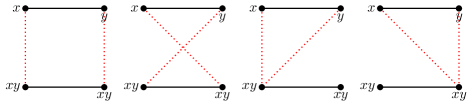
Example 3.16.
Let , where is a field, and let be the Koszul complex of and be the cellular resolution supported on the same cell complex as but with labels and . Let us consider the possible maps from to . If we want the maps to respect the cellular structure, that is, sending vertices to vertices, we have four possible maps. These are illustrated in the Figure 2.
On the level of resolutions the map is a chain map where every square in the diagram of Figure 3 commutes.
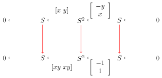
The map has to match up with the mapping of the vertices, so in the first case we have that it maps to and to the other . One can then check that the map making this commute for has to be one of the four maps ,,, or . The first matrix maps the generators in the way we want for the case studied, and the other matrices correspond to the other three cases. It can be checked easily that for any of the four maps there is no that would make the second square commute, this can be done by computing the image of composed with one of the maps and noticing that it can never be inside the image of . This implies that even if the map makes sense topologically on the level of cellular resolutions it does not work.
However, just for the chain complexes one can find maps that behave well algebraically, for example le be given by .Then to make the squares commute one can check that and have to be multiplication by . Similarly we can choose to be given by which would still have the other stay the same. One may also try mapping things to a single generator, so now the map is ( or if one considers the last case). Again the other maps can be found by checking what maps make the squares commute, as we have that we get that , and for we have that is must be the multiplication by .
None of the above maps preserve the degree of the elements between the resolutions. Trying to construct such map one would run into problems with , as it is a map , so the constants in S(-1) have degree , but in the only object of degree 1 is 0. A condition that is reasonable to require from the maps is that the change in the degree is constant when the map is not a zero map, which follows from the commutativity of the squares.
Example 3.17.
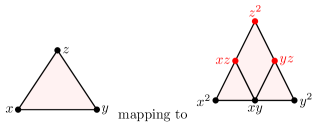
Let . Let be the minimal resolution of the maximal ideal and let be the minimal resolution of . We want to consider the map that as a cellular map sends to the top rectangle of , as shown in Figure 4.
The cellular resolutions of and are displayed in Figure 5.

On the level of the labels the map is a multiplication by , so we know that the map is multiplication by . Then one can choose such that it makes the first square commute. With a little computation one gets the matrix
Clearly, as it consists of entries that are 1, and there is only one entry in each row the map sends the generators of in the first resolution to (some of) the generators of in the second resolution. Because of the ordering of the vertices this map corresponds to sending the vertices of the triangle to the red vertices. Constructing such that the second triangle commutes, and then , we get the maps
These correspond to the map between cell complexes taking the edges and centre of the triangle to the edges and centre of the rectangle in the other complex. One of the edges gets subdivided and this is represented by having two entries in one column in the resolution map.
Example 3.18.
Let and be the same cellular resolutions as in the previous example. Consider the cellular map taking , , and .
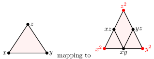
Figure 6 shows this cellular map. If we consider the associated chain map to this, by the compatibility definition we notice that it does not work on the algebraic side. There is no map that would make the squares commute. Hence we do not have a cellular map.
Example 3.19.
Let be the cellular resolution consisting of the direct sum of the two resolutions in the Example 3.18, i.e. the cell complex is the disjoint union and the resolution is
Now consider the projection down to the Koszul complex of . We have standard projections both for the cell complex and the chain complex. More over the two are compatible as the label map generated by the topological projection is the same as the first component in the chain complex projection. Thus, the projection in this case is a cellular resolution morphism.
3.3 The definition of CellRes
Now that we have defined the cellular resolutions and maps between them, we are ready to define the category CellRes.
Definition 3.20.
We define CellRes to be the following data:
-
•
A class of objects consisting of cellular resolutions, coming from any regular CW-complex.
-
•
A set of morphisms for any pair of objects and with individual maps given by the compatible pairs .
Proposition 3.21.
The defined data of CellRes is a category.
Proof.
With this definition of morphisms, for every pair of cellular resolutions and there is a set (possibly empty) of maps. There also exists an identity morphism for every cellular resolution , where is the identity map of chain complexes on the resolution and is the identity map on the cell complex is supported on. We also have that the composition of the morphisms is associative in each component as both composition of chain maps and composition of cellular maps are. ∎
Remark 3.22.
The category CellRes depends on the base ring where the labels are defined, and each ring gives a separate category. In the case the underlying ring is of importance we denote the category by .
For two polynomial rings and with a ring homomorphism we get a functor given by mapping the resolution in to the resolution in by the induced map on the free modules. The morphisms only change the chain map according to the induced module map and the cell map stays the same as the topological structure does not change.
3.3.1 Subcategories of CellRes
The category CellRes has many subcategories. Depending whether the restrictions are on the morphisms or objects, subcategories can allow us to study some subsets of cellular resolutions. We mention here few of the most commonly considered types of cellular resolutions.
Restricting the cellular resolutions to those coming from just labeled simplicial complexes gives a subcategory of CellRes defined on simplicial complexes. This subcategory is full as all the morphisms are there. Every monomial ideal has a resolution in the category of cellular resolutions coming from simplicial complexes thanks to the Taylor resolution.
Another possibility is to just look at the category of minimal cellular resolutions. We know that most of the constructions given in the following sections are not closed in this subcategory as they give non-minimal resolutions.
4 Properties of the Category CellRes
In this section we present some observations for the category CellRes. Among these are definition and results on homotopy on cellular resolutions, and forgetful functors to Top and .
Proposition 4.1.
The cellular resolution
supported on the empty complex is the initial object in the category CellRes.
Proof.
The empty complex is defined to have the label 1, and has a cellular complex
which is also the resolution of the ideal .
From this resolution we have a map to any cellular resolution by taking the chain map to be the zero map for when , and by defining to be the identity. The cellular map is the embedding of the empty complex to the cell complex supporting the resolution . By definition of the initial object, the cellular resolution is an initial object in . ∎
We have a well defined concept of homotopy for both cell complexes and chain complexes. The next definition lifts these definitions to CellRes.
Definition 4.2.
Let be two morphisms in CellRes. We say that is homotopic to if the components are homotopic, i.e. as chain maps and as continuous topological maps.
Homotopies form a nice class of maps in Top. Among the desirable properties is that they satisfy 2-out-of-3 property and 2-out-of-6 property, which are defined below. These also lift to cellular resolutions.
Definition 4.3.
Let be a class of morphisms in a category . Two compasable morphism and are said to satisfy the 2-out-of-3 property if any two of the morphisms , , and are in , then the third is too.
Three composable morphisms ,, and satisfy the 2-out-of-6 property if and are in , then so are ,,, and .
Proposition 4.4.
Homotopy maps form a class of morphism that satisfy the 2-out-of-3 property and 2-out-of-6 property.
Proof.
This follows from that in Top and category, these homotopy properties are satisfied. Hence we get that the homotopies in CellRes also satisfy it as both components satisfy it. ∎
Proposition 4.5.
CellRes is a homotopical category.
Proof.
Take the weak equivalences to be the homotopies defined above. Then this class of morphims contains identities and isomorphism. Moreover, the homotopy in both Top and satisfy the 2-out-of-3 property so, then does the homotopy in CellRes. ∎
Another one of the properties CellRes inherits from Top is the enrichment by simplicial sets. Recall that the enrichment by a monoidal category was defined in the Section 2.1, Definition 2.13.
Proposition 4.6.
The category CellRes can be enriched with simplicial sets.
Proof.
We want to show that for any pair of cellular resolutions and we can assign a simplicial set . We know that the category Top can be enriched with simplicial sets by taking for any pair , the simplicial set where the 0-simplices are the maps between and , the 1-simplices are the homotopies between the maps, and the higher simplices are the higher homotopies.
We can defined the simplicial set in the same way in CellRes. For any pair and take the 0-simplices to be the morhisms between them, the 1-simplices are the homotopies, and the higher homotopies are the higher simplices.
Then the above definition inherits the properties of enriched category from Top. ∎
Proposition 4.7.
The kernel (and cokernel) for the maps in do not exist in general.
Proof.
Let be a morphism of cellular resolutions. By definition, the kernel of a morphism is an object and a map , such that .
From the definition of composition of morphisms in , we have that and . In particular, this means that is the kernel also as a chain complex, and as a requirement for the cellular resolutions it should be a free module. However, we know that the kernel of a module map of free modules is not necessarily free. Thus the kernel may not even be a chain complex of free modules.
Similarly, cokernels do not always exist as the map on the level of modules does not give a free module as the cokernel at homological degree in the chain complex in most cases. Again the examples with cokernel existing in the category are from cases with multiple connected components. ∎
Remark 4.8.
Because the category does not contain all the kernels and cokernels we know that it is not abelian.
We have two important forgetful functors from the category of cellular resolutions, one to chain complexes and one to topological spaces.
Definition 4.9.
Let be a covariant functor taking a resolution
to a chain complex with the same -modules and differential maps as in . The morphism between two cellular resolutions and gets mapped to the chain map under .
Definition 4.10.
Let be a covariant functor, given by mapping to the unlabeled cell complex supporting the cellular resolution. Then maps a morphisms to the cellular map .
Proposition 4.11.
The forgetful functors and preserve weak equivalences, that is, they are homotopical.
Proof.
This follows directly from the definition of the functors and the weak equivalences on CellRes.∎
5 Mapping cones and cylinders
The mapping cone (and mapping cylinder) construction for chain complexes is modeled after the mapping cones (and cylinders) for topological spaces. This means that the two constructions are similar and one would expect both of them to work for cellular resolutions, which is indeed the case.
5.1 The mapping cone
Since we have that mapping cones are very similar in and Top, we can use the definition of on cellular resolutions as well.
Definition 5.1.
Let be a morphism between two cellular resolutions. Then the mapping cone is the chain complex for or with the differential , and .
Remark 5.2.
Here in the mapping cone is equal to only in the case where we do not write down the grading for free modules in the resolution. If the grading is considered then we have a free module for each component of with generators given by the differentials.
Proposition 5.3.
The mapping cone of cellular resolutions is in the category of CellRes.
Proof.
Let be the mapping cone coming from . We have , which is a free module as both and are free modules. The differential satisfies as it is same as for chain complexes. To show the other inclusion, we note that implies that is in the image of and hence by the chain map property of commutative squares for h, we have that is in the image for for . We can write , and we get that . Then the fact is a differential in a cellular resolution implies that , so . Hence it is in the image of .
Let and be the cell complexes of and of , respectively. Consider the mapping cone for the associated cell complexes by the map . It is the cell complex where we have all of , a single point coming from the complex , and then a -dimensional cell for each dimensional cell in . Then the cellular complex for the mapping cone is , and higher degrees , up to the same abuse of notation as in the definition. So we se that this is indeed the same as the chain complex mapping cone, and so it has a cellular structure. ∎
Remark 5.4.
This mapping cone is in most cases not minimal, and can be very far from it.
Remark 5.5.
If the map has the identity map , then the mapping cone will contain label 1.
Proposition 5.6.
The mapping cone for cellular resolutions corresponds to the mapping cones in and Top via the forgetful functor.
Proof.
This construction does match the topological construction for the mapping cone. This is because the cell complex associated to the mapping cone only adds one point for each connected component of and a number of other faces depending on the maps involved, to the cell complex of . Algebraically this can be seen from the fact that the free module in the homological degree 1 is , where generators correspond to the points in the cell complex. ∎
Example 5.7.
Let us consider the cellular resolutions in Figure 7, with the cellular resolution
coming from the complex in the Figure 7, and
from the complex in the same figure. Both have the ideal as their label ideal. The map between the two is identity, and it embeds the minimal resolution to the non-minimal one. Then using the definition of mapping cones we get the resolution
with the maps shown in the Figure 8.


The labeled cell complex associated to this is then the cell complex in Figure 9.
We can see that this cell complex is the same as the topological mapping cone of the embedding of to .
This ”adding a point” property can then be used to construct cellular resolutions from known ones. For the next result we consider cellular resolutions with connected cell complex.
Corollary 5.8.
Let be a cellular resolution for the module . If a map has being a multiplication by a monomial , then the mapping cone will give the resolution of .
Proof.
Let be a morphisms such that is a multiplication by a monomial . We know that the mapping cone is a cellular resolution by Proposition 5.3. Then the label on the ”new” vertex of the mapping cone is given by the map acting on the element 1. Then by definition of , we get . Thus the labels on the cell complex of the mapping cone are . Then by the Proposition 3.9, we have that the mapping cone is the resolution of . ∎
In particular, if one can construct a new morphism to the mapping cone with suitable monomial multiplication, iterating the above process can give specific cellular resolutions. However, in general finding these components proves challenging.
This kind of iterative behaviour of mapping cones was studied by Herzog and Taniyama in [11] for resolutions to construct minimal resolution in a purely algebraic setting. Later on Dochtermann and Mohammadi showed in [8] that the minimal free resolutions from iterated mapping cones of [11] are cellular resolutions.
Definition 5.9.
A monomial ideal with a minimal set of generators and an order on the generators is said to have linear quotients if the colon ideal is generated by some subset of the variables of for all .
We define the set
Proposition 5.10 ([11]).
Let be an ideal with linear quotient with respect to the ordering , and let and . We have the exact sequence
The map is multiplication by . Let denote the graded free resolution of and the Koszul complex of the regular sequence with , and let be a graded chain map lifting . Then the mapping cone gives the free resolution of . Iterating the process we get a graded free resolution of .
Theorem 5.11 ([8], Theorem 3.10).
If the ideal has linear quotients with respect to some order and that the decomposition function is regular, then the minimum resolution obtained via iterated mapping cones is cellular and it is supported on regular CW-complex.
5.2 The mapping cylinder
One can also construct the mapping cylinder of two cellular resolutions. Just like the mapping cone construction, it agrees with both the topological mapping cylinder and the chain complex mapping cylinder.
Definition 5.12.
Let and be two cellular resolutions with labeled connected cell complexes and , and suppose there is a map . Then the mapping cylinder, , is the cellular resolution given by the following data: we set as the topological mapping cylinder is connected, and the other free modules are given by
The differentials of the mapping cylinder are then given by
Proposition 5.13.
The mapping cylinder is a cellular resolution.
Proof.
Taking the topological mapping cone of the labeled complexes and along , and then computing the cellular chain complex for the mapping cone gives us the same chain complex as the above definition. Therefore we know that the mapping cylinder does have a cellular structure.
Next we need to show that the mapping cylinder is indeed a resolution, i.e. that it is acyclic. The kernel of is . It is not hard to see that , and so the chain complex given by the mapping cone is acyclic if the two complexes are acyclic.
To show that this resolution is supported on some cell complex we again consider the case of the associated cell complexes. Take the mapping cylinder for and . Following the definition it is a cell complex with and as subspaces, and for each cell of dimension in , a -dimensional cell in the mapping cylinder. The label of is the least common multiple of the labels of and . Then we can construct the cellular complex of the mapping cone and get , , and . Thus we see that it is the same as the mapping cone defined for cellular resolutions, and hence there is a cellular structure. ∎
Example 5.14.
Let us consider the same map and cellular resolutions as in the Example 5.7 (of a mapping cone). For the mapping cylinder we get the resolution shown in the Figure 10.

Since a single mapping cone is a cellular resolution, one can ask whether multiple mapping cones can be glued together to form cellular resolutions. The answer to that is yes, and the result is in Proposition 5.16 below.
Lemma 5.15.
Let and be cellular resolutions, such that both contain the sub-resolution . Then gluing and together along , by identifying the in with the in , gives a cellular resolution.
Proof.
Let be a sub-resolution of both and . Then we can write and for . The differentials in can be written as , and similarly for . Let be the glued cellular resolution. Identifying the two resolutions along gives for and where and . The -module is a direct sum of free modules with differentials . The differentials are made of sums of acyclic differentials, hence they also give an acyclic chain complex.
The above shows that is a resolution. Now we want to show that it is supported on a cell complex. We note that the resolution has everything corresponding to the cell complex of and to the cell complex of as well. They are connected along . Taking the cell complex obtained by gluing the associated complexes of and along the cell complex of , gives us a cell complex that has as its cellular complex. ∎
Proposition 5.16.
Let be a finite diagram of cellular resolutions. Then gluing mapping cylinders into , gives a new cellular resolution.
Proof.
Let be a finite diagram of cellular resolutions. Then for each morphism in it, we can construct the mapping cylinder. By Proposition 5.13 the mapping cylinders are cellular resolutions. In the mapping cylinder of both and are sub-resolutions. Lemma 5.15 tells us that any two mapping cylinders glued along or are a cellular resolution. Thus by gluing the mapping cylinders together along the common components of one at a time gives us a cellular resolutions, while the components are not connected.
In the case we have a cellular resolution , obtained by gluing mapping cylinders, that contains two (or more) copies of a cellular resolution we can glue the cellular resolution to itself along the sub-resolution . This corresponds to the situation where we have more than one map between two objects in the diagram, for example a composition of maps being equal to another map. Because fo this one can view the resolution before gluing consisting of the resolutions , , and two disjoint mapping cones and between them. The piece of the resolution can be written as . Trying to use the approach with the differentials as in Lemma 5.15, we get a chain complex which has with a differential . This chain complex is not acyclic. The differentials will not cover all the elements after homological degree 2. The missing elements in the kernel of the maps come from that after gluing, both mapping cylinders in degree will have elements mapping to the same element of the image of in . To make the glued resolution acyclic, we want to identify the mapping cylinders corresponding to a same map. This is done by adding a free module in homological degree for each of the generators in homological degree of such that maps exactly to the degree modules coming from the mapping cylinder component of a single generator. The added modules provide the needed elements to the maps to cover the kernel elements coming from the mapping cylinders. Hence we get an acyclic resolution after the glueing and identifying the mapping cylinders.
On the supported cell complex the gluing without identifying the mapping cones corresponds to having a hole in the complex. Adding the extra pieces is equivalent to adding in an -cell for each -cell in the complex of such that the -cells in the mapping cylinder corresponding to an -cell form the boundary for the -cell.
So now we have that gluing the mapping cylinders together one common component at a time gives a cellular resolution at each step. With the assumption that our diagram is finite, we have that eventually each common component of the mapping cylinders has been glued, and we have a cellular resolution. ∎
Definition 5.17.
Let be a diagram of labeled cell complexes. Then we take their gluing along the maps to be the same topological cell complex as with the usual gluing of complexes and the labels on the vertices to be the least common multiple of all the labels of the vertices that are glued together.
Proposition 5.18.
Let be a morphism of cellular resolutions. Then gluing to along the chain map f of the morphism gives a cellular resolution.
Proof.
Let be a morphism of cellular resolutions. Let us consider the gluing along f given by , where if we have . Firstly we show that is a free module. The map maps each generator of to an element of or to 0. This means that each element can be written as a combination of the basis elements of , so is a free module. Also this gives that the differentials are just the same as in . Furthermore, as is a cellular resolution, also has a labeled cell complex and is a cellular resolution. ∎
6 Products, coproducts, and the tensor product
6.1 The product
We know that the categories Top and have different types of products. In it is (in a finite case) the same as the direct sum, whereas in Top we get a connected cell complex instead of the disjoint union. This tells us that we cannot use either of the known definitions for the product in CellRes, as this would then either not preserve the topological structure or not preserve the algebraic structure of a product.
We can, however, lift the construction of the topological product with trivially labeled cell complex to CellRes.
Definition 6.1.
Let be a cellular resolution supported on the cell complex , with and differentials . Let be the cellular resolution coming from the -simplex with labels 1.
The product of a cellular resolution with , is the cellular resolution , with and
The differential of the product in the matrix form is given by
where denotes the diagonal matrix where each diagonal entry is , and denotes the matrix of the differential of the simplex with identity map entries.
The cell complex supporting the product is the topological product of and the -simplex. The orientation of the product complex is given by each copy of having the same orientation as and each -simplex having the same orientation and the new faces being ordered by the order of the one dimension lower faces of .
The projection from to is a pair where is the standard topological projection and is a compatible chain map with . The projection from to is a compatible pair where is also the standard topological projection, and is a compatible chain map sending all labels to 1.
Remark 6.2.
The above is not a product in the usual sense, as the map in the universal property is not unique. However, the maps are unique up to homotopy and this suffices for our purposes.
Example 6.3.
Let . Let be the cellular resolution associated to the Koszul complex of . Then consider the product with . Using Definition 6.1, we get that the resolution is
with maps , and . By the definition of a product, if we have something mapping to the two components, we should have a map to the product, too, such that the maps commute. We can take as the cellular resolution mapping to itself and to . Then we have a map from to the product. On the level of cell complexes, we can draw a picture of the product diagram, which is shown in Figure 11.
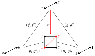
The red part of the diagram marks where a continuous map would map to in a product, if we consider the topological product for the cell complexes. Clearly, is not a cellular map, as it maps the edge of to a higher dimensional face. So one can not take the topological map as a component for the morphism making the diagrams commute in . We know that the vertices have to be mapped as in the drawn red map to make the diagram commute, so we can choose a cellular map that maps the vertices in this way. This leaves two different options how we map the edge, up or down from the red line, and with just the requirement to make the diagram commute, there is no clear choice between the two options.
This non-uniqueness can also be seen algebraically. We refer to the left and the right side of the diagram in the Figure 11. To make the left side diagram commute on with and , we see that . Then also using that the right diagram must commute we get . Finally to choose the map , we run into the situation where both and make the diagram commute. Hence the product defined in Definition 6.1 does not give a product in the category-theoretic sense, because the map in the universal property is not unique. However, the choices are homotopic to each other, so the map is unique up to homotopy.
These choices in choosing the map to the product arise at level where the map of the topological product map subdivides a cell.
Proposition 6.4.
Let be the product of cellular resolutions and . Let be a cellular resolution mapping to both and . Then the vertex map from the cell complex supporting to the cell complex of is well-defined and compatible with a module map.
Proof.
Let be the cell complex supporting , and let be the cell complex supporting . Let be the continuous map between cell complexes that makes the topological product diagram commute.
In the dimensions where does not subdivide cells it satisfies the conditions of a cell map. Since the other maps in the commutative diagram are cellular, we know that they map vertices to vertices. Then commutativity implies that must map vertices to vertices. Let us denote by the cellular part of .
Similarly, if we just consider the chain map part , we can compute due to commutativity of the triangle between , and . The map is compatible with the cellular map , which again follows from the commutativity of the diagram. ∎
Remark 6.5.
We note two things about the nature of the subdivision in the product .
-
(1)
In the product, the only subdivided cells are the ones not in either one of the components of the product.
-
(2)
Subdivision maps a face of of dimension to a face in of dimension , and the higher dimensional cell is divided into two parts.
Proposition 6.6.
Let be the product of the cellular resolutions and . Let be a cellular resolution mapping to both and . Denote the cell complexes the cellular resolutions are supported on , , and .
Let be the continuous map that makes the topological product diagram commute. Then there exists a cellular map that is homotopic to the unique topological map in the topological product.
Moreover, the cellular map together with a compatible chain map forms a morphism that gives commutative product diagram in CellRes.
Proof.
From the cellular approximation theorem we know that if we have a continuous map between two CW-complexes, then there exists a cellular map that is homotopic to the continuous map. In our case take the continuous map to be from to in the product, then there exists a cellular map . We know that the cellular approximation to the unique topological map is equivalent to up to the first subdivision of cells in . Let be the dimension of the faces where we get the first subdivision, and let be one such face. From our observations in Remark 6.5 we have that is contained in some cell of dimension , and the projection of that cell is . Since is of dimension and it is ”purely a product face”, then the boundary also maps to under the projection. Moreover, the boundary of gets mapped to the boundary of by continuity, and divides into two parts. Combining these observations we can choose the boundary (with only entire faces chosen) of one of the halves of to be . Then commutes with the other maps in this dimension. Furthermore as is a cellular map, the higher dimensional cells will also satisfy the commutativity requirements due to mapping in the same way as the -dimensional one. On the algebraic side we can then construct the algebraic map based on . ∎
Proposition 6.7.
The product construction gives a product up to homotopy, that is, is a cellular resolution, there is a map to each component of the product from and it satisfies the universal property up to homotopic maps.
Proof.
To show that the product is a cellular resolution, we only need to show that it is an acyclic chain complex as it is the cellular complex of a labelled cell complex. A simple computation on the defined differentials shows that , so the . Let us consider the kernel of the map . We know that the kernel of each component of is contained in the image as they are from cellular resolutions, and so the whole kernel is. Thus we have that the product construction with gives a cellular resolution.
A product must also satisfy the universal property, so let us consider the cellular resolution with the property that maps to both and . As the product has the same cell complex as the topological product, and the projection maps associated to it are also same for the topological products, we know that we have a cellular continuous map from the cell complex of to the product by Proposition 6.6.

By the same proposition we have that the diagram in the Figure 12 commutes for any of the cellular approximations and a compatible chain map. Hence we get that the universal property holds up to homotopic choice of a CellRes morphism. ∎
The construction used in the product can be applied to any two cellular resolutions. However the resulting cellular resolution may not satisfy any of the product properties. In the case that the two cellular resolutions share labels with greatest common divisor other than 1, we do not even get well defined maps from the product construction to the components.
Proposition 6.8.
Let be the set of labels in the product construction for two cellular resolutions and with label sets and , respectively. If the maps from to and are generated by maps coming from the topological product of the cell complexes of and and they are compatible with chain maps between the resolutions, then we get that is a product in CellRes.
Proof.
If the ideals associated to and do not have independent generator sets from each other, that is the generators between the sets have no non-trivial common divisors, then the label maps cannot be compatible. This follows from that we cannot construct a map from the ”product” to and .
Let us assume that the genertor sets and are independent of each other. Then the associated cell complex is still the topological product, so we can take the morphisms as in the case but the distinction that the projection from to maps all labels from to 1, and labels from to 1 with the other projection.
Then we can apply the same arguments as in the product case to construct the cellular resolution using the cellular approximation to the topological product map. ∎
Remark 6.9.
The above proposition gives that we have the product with any cellular resolution with cell complex having labels 1.
6.2 The coproduct
Next we move on the coproduct. Unlike with the product, both in Top and the (finite) coproduct is a disjoint union. Thus the construction can be lifted to celluar resolutions directly.
Definition 6.10.
The coproduct, , of two cellular resolutions and is a direct sum of the cellular resolutions, so we have . The labeled cell complex supporting the coproduct resolution is the disjoint union of the two labeled cell complexes, which also is the coproduct of cell complexes.
Proposition 6.11.
The coproduct defined in Definition 6.10 is a cellular resolution and satisfies the definition of category-theoretical coproduct.
Proof.
Let be the coproduct of and as defined above. The direct sum of two cellular resolutions is still a cellular resolution, as direct sums of chain complexes preserve exactness. The differentials are just the maps for the disjoint cell complex. The maps from and to are embeddings of the cellular resolutions.
Lastly, for this to be a coproduct we need the universal property. Let be a cellular resolution such that both and map to it. Since Definition 6.10 is the same for chain complexes and topological spaces, we have a unique topological map and a unique chain map from to . To show that these two maps are compatible with each other and form a unique CellRes morphism consider the diagram of the coproduct. We have commutativity so the maps , and satisfy and . Let be a cell in the cell complex of and the generator associated to it. From the cellular resolution maps and we know that corresponds to the cell , and corresponds to the cell . Commutativity tells us that will satisfy compatibility for all elements in coming from . Since the arguments also hold for , we get that is a cellular resolution map.∎
Proposition 6.12.
The category CellRes has all finite coproducts.
Proof.
We have that the coproduct of any two cellular resolutions exists. Then one can compute the coproduct of finitely many cellular resolutions by taking the coproduct inductively. At each step this is still the coproduct of two cellular resolutions, and so we have that each finite coproduct is in CellRes. ∎
Remark 6.13.
We only consider finite cellular resolutions, so an infinite coproduct would produce an infinite cellular resolution and hence we do not have infinite coproducts.
Definition 6.14.
Let be a set, and a cellular resolution. Then the repeated coproduct over , , is called the copower (over ) and denoted by such that the morphisms satisfy and it is natural in .
6.3 Tensor product
The category can be given a tensor product structure.
Definition 6.15.
Let and be any two cellular resolutions with and . The tensor product of the two resolutions, , is given by
The differential is given by the matrix for the standard tensor product of chain complexes, with entries simplified such that each column has greatest common divisor 1.
As defined above the tensor product can be written as a bifunctor . Also the modules involved are free modules, so , and corresponds to the element .
Remark 6.16.
The definition of the tensor product is almost the same as for chain complexes. Indeed on the object level they are the same but the differentials in the tensor product of would not give an acyclic complex.
Proposition 6.17.
The labeled cell complex of the tensor product of and is the join of the complexes of and .
Proof.
We can compute the associated cell complex from the defined cellular resolution for the tensor product. We see that the vertices stay the same and that the cell complexes of and are contained in the tensor product. The new edges are formed to connect vertices of the components and respectively the higher dimensional faces. So this is the join of the complexes. ∎
Remark 6.18.
In the case that the label ideals of and have coprime generators the differential in the tensor product is just the usual differential of the tensor product of chain complexes.
Proposition 6.19.
The tensor product defined as above is a cellular resolution.
Proof.
Firstly, we know that the chain complex defined by the tensor product is made of free modules (tensor product of free modules is free). We also have that it is supported on a cell complex, so it has a cellular struture. It remains to show the tensor product is acyclic. The matrix for the differential consists of submatrices, where the th matrix, denoted by , is the map from to and is of the size . The matrix has nonzero entries if and only if or . Let us look at the case in more detail. The positions of the nonzero entries come from the map identified with a matrix. The image applied to is identified with the element
This can be seen coming from a matrix where the rows are indexed by and the columns by , and the entry is nonzero if and only if and it is given by .
The map is given by the matrix with the same row and column index as above, and the entries are zero unless . Then the entry is given by where is the th generator of the module coming from the labelling. From this form one can see that the acyclicity is preserved in the component of the differential. We can apply the similar argument to the case , and also get that it preserver acyclicity. Therefore, the tensor product resolution is acyclic.∎
With the defined tensor product for cellular resolutions we have the following result. The reader may refer to Section 2.1 for the categorical definitions.
Proposition 6.20.
The tensor product defined above gives the category CellRes a monoidal structure.
Proof.
We take the tensor product as defined in Definition 6.15 to be our bifunctor . Take the void resolution, , as the object of the monoidal category. Define a natural transformation . For to be a natural isomorhism we need that is an isomorphism. Using the definition of the tensor product and that on module level it is the same as for the chain complexes, we have that
Hence we get that defines a natural isomorphism.
Let us consider the natural transformations and . By the definition of natural transformation we have the commutative diagram for , and for any and any morphism ,
Since if and 0 otherwise, we can compute that for any . It is not hard to see that is an isomorphism in CellRes, and that is a natural isomorphism. The same argument can be used for to show that it is also a natural isomorphism.
A simple computation shows that the triangle and pentagon equalities are also satisfied. ∎
Example 6.21.
Let be the cellular resolution
coming from the complex in Figure 13, and let be the cellular resolution
from the complex in Figure 13.

Then their tensor product is the cellular resolution
with differentials
The join of the cell complexes in Figure 13 is four dimensional cell complex.
7 Limits and colimits
As with the earlier constructions, we know what the limits are for cell complexes and chain complexes. In the case of limits, and later on colimits, we also know that the categories Top and are (co)complete, thus they have all limits and colimits. However we know that in general limits do not exist in CellRes as we do not have the products in general.
Definition 7.1.
A diagram in is a functor where is a finite indexing category.
Remark 7.2.
When denoting the cellular resolutions in diagrams we use the superscript with . This is to avoid confusion with the homological degree of the components of the cellular resolution.
7.1 Limits
In general, we can show that the limits in chain complexes as given in Definition 7.3 preserve acyclicity, however just being acyclic is not enough to be a cellular resolution.
Definition 7.3.
Let be a diagram in , and denote the cellular resolutions in it by . By definition the limit of the diagram, if it exists, is the cellular resolution that has a morphism to each , such that any triangles commute, and must satisfy the universal property.
The product behaviour would suggest problems with the limit when there is non-connected cellular resolutions in the diagram, so for now we restrict ourselves to inverse limits rather than the general limits.
An inverse limit is a limit where the diagram is an inverse system.
Definition 7.4.
The inverse system is given by the following. Let be a directed poset. Let be a collection of cellular resolutions with morphisms for all , such that is the identity and for all .
We have that for particular class of inverse limits they always exist in CellRes.
Proposition 7.5.
Let be a finite inverse system of cellular resolutions such that the underlying poset is a tree. Then the inverse limit of exists in CellRes.
Proof.
Let be an inverse system in CellRes, and let be the index of the upper bound element in the poset. Let denote its limit as a chain complex. Then we know that is the inverse limit of modules , written explicitly as
Since the poset is a tree, and for all , we can write the module as
Furthermore we know that the differentials are the same as in , due to the squares of the maps from to the diagram being commutative. So we have that .
Next we want to show that also satisfies the commutativity requirements for the cellular maps and universal property. The map from to is . Then by the composition rules for the maps defined in Definition 7.4 we have that for any , . So satisfies the commutativity condition of an inverse limit. Let be a cellular resolution, and suppose that maps to every component of . Again any triangles we have must be commutative, so in particular if and , then . If maps to all maps must factor through it, in particular is then a map composed with identity we get . With the earlier observation of factoring maps we get that satisfies the universal property.∎
7.2 Colimits
The situation with colimits is better than with limits. We do infact have (finite) colimits in CellRes. The following proposition show the existence and also recalls the definition of colimit.
Proposition 7.6.
Let be a finite diagram in CellRes. Let be the colimit of the diagram as colimit of chain complexes with maps , and let be the topological colimit of the associated cell complexes in the diagram with maps . Then is the cellular complex of , together with maps .
Proof.
Let be a finite diagram of cellular resolutions. Let be the cell complex of the cellular resolution, and let be the topological colimit of the ’s of the diagram .
We view as the space obtained by gluing the cell complexes together with the labels given by Definition 5.17. The dimension faces of are given as the disjoint union of the dimension faces of ’s. One then identifies the with if there is such that . By definition the cellular free complex of is given as . We can write the free module as
where if due to the gluing observation above. Identifying the free modules with one generator is equivalent to identifying their generators . We can write this as
Let be the chain complex colimit of . By definition of colimit in ,
Since the modules come from the cellular resolutions, we know that . If there is a map then we know that the generators map to generators (with multiple ). Thus
Now it is not hard to see that and are the same module. Therefore we have that is the cellular complex of .
As the cellular free complex is both the colimit in Top and we get that it inherits the colimit structure from those categories. What remains to show is that it in fact is a cellular resolution, which means we want to show it is acyclic. Let denote the colimit as given above. As with the limit we can draw a diagram with and cellular resolutions shown in Figure 14.

Let . Using diagram chasing on the diagram in the Figure 14, we get that . Therefore is acyclic and hence a cellular resolution.∎
As a natural corollary to the existence of colimit we have the following.
Corollary 7.7.
CellRes is a finitely cocomplete category.
Proof.
As the above Proposition 7.6 holds for any finite diagram of cellular resolutions that has both limit as chain complex and cell complex, we get that we have all finite colimits in CellRes since Top and contain all colimits. Thus CellRes is a finitely cocomplete category.∎
8 Homotopy colimits
We begin with an example of homotopy colimit for the cell complexes.
Example 8.1.
Let be a diagram of three cellular resolutions ad with the cell complexes as in the Figure 15.

The resolutions are a follows: is , is , and is . The map from to is the identity embedding and the map from to is the embedding by multiplying with . Computing the topological homotopy colimit by gluing in mapping cones we get the labeled cell complex in the Figure 16. This cell complex has the cellular complex
with maps
From the maps we can see that the cellular complex is acyclic, hence a resolution.

The previous example motivates us to lift the gluing mapping cylinders definition to CellRes.
Definition 8.2.
Let be a diagram in CellRes with finite indexing category . Let and be resolutions in , and let us denote by the morphism between them if we have a map in . We have a mapping cylinder for each morphism . The th piece of the mapping cylinder is given by , with differentials .
Then the homotopy colimit obtained by gluing in mapping cylinders to the coproduct is the resolution with -th piece
with differentials
Recall that Proposition 5.18 states that gluing in mapping cylinders into a diagram is a cellular resolution. Therefore the above definition also is a cellular resolution.
The homotopy colimit as defined in Definition 8.2 can easily give a very large cellular resolution that is far from minimal. However, it can be homotopy equivalent to a smaller one. For instance in Example 8.1 we could remove the middle square without changing any important properties.
Recall from topology that the homotopy colimit can be defined as the direct sum quotient by some relations (see Definition 2.24).
This then gives a second definition for the homotopy colimit in CellRes. First we need to define the geometric realization in CellRes.
Definition 8.3.
Let be a simplicial set. We define the geometric realization of in CellRes to be the free resolution coming from the geometric realization of in Top with labels 1 on each vertex.
Definition 8.4.
Let be a finite small category and let be a diagram in CellRes. Let and be resolutions in , and let the morphism between them be denoted by if we have a map in . Then we define the homotopy colimit to be the direct sum
quotient by a relation . Here is the geometric realization of the nerve of the category under , , and is the element in the diagram associated to the element . We have the maps and , given by
and
for every map , where . Then the quotient is given by the relation .
Example 8.5.
Let the diagram and cellular resolutions be as in Example 8.1 and Figure 15. We use the Definition 8.4 to compute the homotopy colimit for the diagram.
The indexing category has three objects, say and for , , and respectively. We compute the geometric realization of the nerve of the category under each of the objects. Starting with , the simplicial set has chains of length zero coming from the objects and , and . Then it also has chains of length one from and , and the ones coming from identity maps. The higher degree ones are given by adding identity maps to the length one chains. Then is given as a cell complex by . Computing this, we see that the parts coming from the identity maps are identified to a point, and the lower ones give one directed edge for each non-identity map. We get that the cell complex is . The resolution for it is . Similarly, we get that , and they have the resolution .
Next we have the disjoint union of
Each of the products is with trivially labeled cellular resolution. Thus they exist and are cellular resolutions. We know that the generators of the product, and also the labels of the associated cell complex are coming from the in this case. Then we take the quotient by the relation where
Note that if we have a map , then . Expicitly the identification of the ”copies of ” in the part of coming from are glued to along the map . We do the same gluing for all the maps in . After the identification we have the cellular resolution
with the same maps as in Example 8.1.
Proof.
Since both definitions are lifted from Top, we know that the underlying cell complexes associated the cellular resolutions are the same.
Starting with Definition 8.2, let us consider the case of maps from . The mapping cylinder for can be thought of as the disjoint union of and quotient by the relation . We also need to glue along all the mapping cones containing , and if we have a composition then along those as well. Writing this as the single mapping cylinder above, we have the disjoint union of , one for each map from , and a copy of for each maps to. The quotients are along all glued together, for each map, and if we have a map then we identify with . This is the same as taking the product of with simplicial space that records the map structure, i.e. precisely , and gluing the vertices of corresponding to the map with the of while identifying and via .
Taking the above product for all the in the diagram, and gluing them together by the mapping cylinder rules then gives us that we have gluing between and if we have a map . Then the identification of the gluing is given by
which recovers the relation . Therefore it is equivalent to Definition 8.4, and the two definitions give the same cellular resolution. Moreover, this shows that Definition 8.4 does give a cellular resolution.∎
9 Morse theory and simple homotopy theory
9.1 Morse theory for cellular resolutions
In this section we want to look at Morse theory for cellular resolutions. Recall that the idea of discrete Morse theory is to collapse cells to reach a smaller cell complex with the same homology, and similarly in algebraic morse theory. In the case of cellular resolutions, Morse theory forms an useful tool ”remove” the non-minimal part of the resolution by collapsing it. We illustrate this in the following example.
Example 9.1.
Let be the filled in triangle with vertex labels , see Figure 13 cell complex . The has a Taylor complex
Both the face poset of and the graph , defined in Section 2.4.2, have the directed graph shown in Figure 17.

Let us take the single edge marked with 1 as the Morse matching. Then we can compute the chain complex coming from this with algebraic Morse theory
with differentials
This resolution has the cell complex of Figure 13 as its cell complex. This is exactly the same cell complex one gets by doing discrete Morse theory on .
The first results on the discrete Morse theory of cellular resolutions were in paper by Batzies and Welker [1], and they have been later applied in other works, for example in [13] to construct an algorithm for finding cellular resolutions closer to the minimal one.
One of the main concerns when applying Morse theory to cellular resolutions is whether the resulting complex is still a cellular resolution. In a case with restricted collapses this was solved by Batzies and Welker.
Theorem 9.2 ([1]).
Let be a complex that supports a cellular resolution, and let be a Morse matching on this complex. If only matches cells with the same labels, then the Morse complex also supports a cellular resolution of the same ideal.
Only matching cells with the same label is a strong restriction on what kind of matchings we can make. Algebraically this is the same as only choosing isomorphisms for the matching, which is indeed the case in algebraic Morse theory as we have seen in the Section 2.4.2.
Proposition 9.3.
Let be a cellular resolution with a cell complex . Let be a Morse matching on the face poset of (or the graph ). Suppose that only matches cells with the same labels. Then is a Morse matching also on (or on the face poset of ). Furthermore, is the cellular complex of .
Proof.
Note that the face poset of and the graph of are the same directed graph up to the labels on the vertices. The vertex in corresponding to cell is the same vertex in with the free module having generator corresponding to .
Let be a Morse matching on , and suppose it only matches cells with the same labels. We can consider the matching on . Since the underlying graph is the same as in , is a matching on without any directed cycles when the edges in are reversed. The vertices in come from the summands at each homological degree, so by definition a vertex is where is the fine graded degree of the label of some . By the same label condition for edges in , we have that if the edge matches and , then the cells and have the same label. This gives that . Then the corresponding map in between and is an isomorphism, as they are the same free module. It follows that is a Morse matching on as well.
On the other had, if is a Morse matching on , we again get directly that it is matching on without directed cycles of the edges in are reversed. also only matches free modules that are isomorphic, and we know that if then and have the same label. So the corresponding vertices in of a matched edge in are cells with the same label. Thus is a Morse matching on that only matches cells with the same labels.
We have established that the algebraic and same label cell matchings are the same. Let be the homotopic chain complex of after the Morse map and let be the cell complex after collapses on . One way to see that is the cellular complex of is to consider their poset diagrams. Since they come from the posets of and , we know that the vertices correspond to each other, and the remaining vertices have not changed. As the same Morse matching is applied to both and , the resulting posets are the same up to vertex labels. Lastly we know from Theorem 9.2 that supports a resolution, and as is the cellular complex of , we have that is a cellular resolution. ∎
Theorem 9.4.
Let be a cellular resolution with a cell complex , and let be a Morse matching on them. Let be the chain map from to , and let be the cellular strong deformation retract of coming from Morse theory. Then the pair formed of the Morse maps is a morphisms in CellRes.
Proof.
A single edge in the Morse matching corresponds to a collapse, and we can do these collapses one by one. Thus we may assume that the Morse matching in this case is a single edge. We want to show that f and are compatible, so that they form a morphism in CellRes.
Let be a Morse matching with a single edge that generates the maps. Let us denote by and the generators of the vertices in , and with and the cells corresponding to the vertices of . For any unmatched vertices, in both and , the maps f and act on these vertices as an identity. It follows from the definition of the identity that the maps satisfy the compatibility for those parts. In particular, the chain map has for any , and cells of lower dimension than map by identity.
Let us focus on the maps , and on cells of dimension and . We will first show that is a linear combination of other generators of the modules maps to. Since we have explicit description of the resolution , we have that
As noted before, is identity on . So we only need to compute . From the definition of the chain map we have that . Let be the generators of where and there is an edge from to . From the differentials and their composition we have that for some . Combining this with the commutativity, we get that . Similarly, we can show that using the properties of differentials and the commutative squares.
On the topological side, deformation retracts and to . So they both map to the intersection of boundary of and . Then will map to a smaller dimensional cells, so a compatible chain map maps the generator associated to to 0 in degree , which we have with . These conditions also give that either maps to cells of the same dimension or to lower ones. In the former case, we get that these are the cells corresponding to the algebraic generators , and we have the compatibility that we want. In case , we then know there are no other -cells on the boundary of . This also implies that only maps to one element, . Thus we get that , so the two maps are compatible. ∎
9.2 Simple homotopy theory
Having the morse maps as morphisms in CellRes allows us to define simple homotopy for cellular resolutions. For classical simple homotopy theory the reader may look up the book by Cohen [6].
In the language of simple homotopy theory, a Morse matching with a single edge is an elementary collapse. We have also the elementary expansion.
Definition 9.5.
Let and be cellular resolutions. Suppose that there is an elementary collapse from to . Then we say that expands to by an elementary expansion, or that there is an elementary expansion from to . A finite sequence of elementary collapses and elementary expansions is called a formal deformation.
Now we can define the simple homotopy equivalence for cellular resolutions.
Definition 9.6.
Let and be cellular resolutions. Let be a formal deformation. Then we get that and are simple homotopy equivalent.
References
- [1] Ekkehard Batzies and Volkmar Welker. Discrete Morse theory for cellular resolutions. J. Reine Angew. Math. 543 (2002), 147-168.
- [2] Dave Bayer, Irena Peeva, and Bernd Sturmfels. Monomial resolutions. Math. Res. Lett. 5 (1998), no. 1-2, 31-46.
- [3] Dave Bayer and Bernd Sturmfels. Cellular Resolutions of Monomial Modules. J. Reine Angew. Math. 502 (1998), 123-140.
- [4] Francis Borceux. Handbook of categorical algebra 1. Encyclopedia of Mathematics and its Applications, 50. Cambridge University Press, Cambridge, 1994. xv+345 pp.
- [5] Francis Borceux. Handbook of categorical algebra 2. Encyclopedia of Mathematics and its Applications, 51. Cambridge University Press, Cambridge, 1994. xvii+443 pp.
- [6] Marshall M Cohen. A course in simple-homotopy theory. Graduate Texts in Mathematics, Vol. 10. Springer-Verlag, New York-Berlin, 1973. x+144 pp.
- [7] George E. Cook and Ross L. Finney. Homology of cell complexes. Princeton University Press, Princeton, 1967.
- [8] Anton Dochtermann and Fatemeh Mohammadi. Cellular resolutions from mapping cones. J. Combin. Theory Ser. A 128 (2014), 180–206.
- [9] Alexander Engström and Patrik Norén. Cellular resolutions of powers of monomial ideals. arXiv:1212.2146
- [10] Robin Forman. A user’s guide to discrete Morse theory. Sém. Lothar. Combin. 48 (2002), Art. B48c, 35 pp.
- [11] Jürgen Herzog and Yukihide Takayama. Resolutions by mapping cones. (English summary) The Roos Festschrift volume, 2. Homology Homotopy Appl. 4 (2002), no. 2, part 2, 277-294.
- [12] Michael Jöllenbeck and Wolkmar Welker. Minimal resolutions via algebraic discrete Morse theory. Mem. Amer. Math. Soc. 197 (2009), no. 923, vi+74 pp.
- [13] Josep Àlvarez Montaner, Oscar Fernández-Ramos, and Philippe Gimenez. Pruned cellular free resolutions of monomial ideals. arXiv:1701.01134
- [14] Saunders Mac Lane. Categories for the Working Mathematician, second edition. Graduate Texts in Mathematics, 5. Springer-Verlag, New York, 1997. 314pp.
- [15] William Massey. Singular homology theory. Graduate Texts in Mathematics, 70. Springer-Verlag, New York-Berlin, 1980. xii+265 pp.
- [16] Ezra Miller and Bernd Sturmfels. Combinatorial Commutative Algebra. Graduate Texts in Mathematics, 227. Springer-Verlag, New York, 2005. 417 pp.
- [17] Steven Sam and Andrew Snowden. Gröbner methods for representations of combinatorial categories. J. Amer. Math. Soc. 30(2017), no. 1, 159-203.
- [18] Horst Schubert. Topology. Allyn and Bacon, Inc., Boston, 1968. 358 pp.
- [19] Emil Sköldberg. Morse theory from an algebraic point of view. Trans. Am. Math. Soc. 358 (2005), no. 1, 115–129.
- [20] Mauricio Velasco. Minimal free resolutions that are not supported by a CW-complex. J. Algebra 319 (2008), no. 1, 102–114.
- [21] Volkmar Welker, Gunter Ziegler and Rade Zivaljevic. Homotopy colimits-comparison lemmas for combinatorial applications. J. Reine Angew. Math. 509 (1999), 117–149.
- [22] Charles A. Weibel. An Introduction to Homological Algebra. Cambridge studies in advanced mathematics, 38. Cambridge University Press, Cambridge, 1994. 450pp.