Analyzing Deep Neural Networks with Symbolic Propagation: Towards Higher Precision and Faster Verification

Abstract

Deep neural networks (DNNs) have been shown lack of robustness, as they are vulnerable to small perturbations on the inputs, which has led to safety concerns on applying DNNs to safety-critical domains. Several verification approaches have been developed to automatically prove or disprove safety properties for DNNs. However, these approaches suffer from either the scalability problem, i.e., only small DNNs can be handled, or the precision problem, i.e., the obtained bounds are loose. This paper improves on a recent proposal of analyzing DNNs through the classic abstract interpretation technique, by a novel symbolic propagation technique. More specifically, the activation values of neurons are represented symbolically and propagated forwardly from the input layer to the output layer, on top of abstract domains. We show that our approach can achieve significantly higher precision and thus can prove more properties than using only abstract domains. Moreover, we show that the bounds derived from our approach on the hidden neurons, when applied to a state-of-the-art SMT based verification tool, can improve its performance. We implement our approach into a software tool and validate it over a few DNNs trained on benchmark datasets such as MNIST, etc.

1 Introduction

During the last few years, deep neural networks (DNNs) have been broadly applied in various domains including nature language processing [1], image classification [16], game playing [27], etc. The performance of these DNNs, when measured with the prediction precision over a test dataset, is comparable to, or even better than, that of manually crafted software. However, for safety-critical applications, it is required that the DNNs are certified against properties related to its safety. Unfortunately, DNNs have been found lack of robustness. Specifically, [30] discovers that it is possible to add a small, or even impcerceptible, perturbation to a correctly classified input and make it misclassified. Such adversarial examples have raised serious concerns on the safety of DNNs. Consider a self-driving system controlled by a DNN. A failure on the recognization of a traffic light may lead to a serious consequence because human lives are at stake.

Algorithms used to find adversarial examples are based on either gradient descent, see e.g., [30, 2], or saliency maps, see e.g., [23], or evolutionary algorithm, see e.g., [22], etc. Roughly speaking, these are heuristic search algorithms without the guarantees to find the optimal values, i.e., the bound on the gap between an obtained value and its ground truth is unknown. However, the certification of a DNN needs provable guarantees. Thus, techniques based on formal verification have been developed. Up to now, DNN verification includes constraint-solving [24, 15, 18, 8, 20, 34, 6], layer-by-layer exhaustive search [12, 33, 32], global optimization [25], abstract interpretation [10, 29, 28], etc. Abstract interpretation is a theory in static analysis which verifies a program by using sound approximation of its semantics [3]. Its basic idea is to use an abstract domain to over-approximate the computation on inputs. In [10], this idea has first been developed for verifying DNNs. However, abstract interpretation can be imprecise, due to the non-linearity in DNNs. [28] implements a faster Zonotope domain for DNN verification. [29] puts forward a new abstract domain specially for DNN verification and it is more efficient and precise than Zonotope.

The first contribution of this paper is to propose a novel symbolic propagation technique to enhance the precision of abstract interpretation based DNN verification. For every neuron, we symbolically represent, with an expression, how its activation value can be determined by the activation values of neurons in previous layers. By both illustrative examples and experimental results, we show that, comparing with using only abstract domains, our new approach can find significantly tighter constraints over the neurons’ activation values. Because abstract interpretation is a sound approximation, with tighter constraints, we may prove properties that cannot be proven by using only abstract domains. For example, we may prove a greater lower bound on the robustness of the DNNs.

Another contribution of this paper is to apply the value bounds derived from our approach on hidden neurons to improve the performance of a state-of-the-art SMT based DNN verifier Reluplex [15].

Finally, we implement our approach into a software tool and validate it with a few DNNs trained on benchmark datasets such as MNIST, etc.

2 Preliminaries

We recall some basic notions on deep neural networks and abstract interpretation. For a vector $\bar{x}\in\mathbb{R}^{n}$, we use $x_{i}$ to denote its $i$-th entry. For a matrix $W\in\mathbb{R}^{m\times n}$, $W_{i,j}$ denotes the entry in its $i$-th row and $j$-th column.

2.1 Deep neural networks

Figure 1: A fully connected network: Each layer performs the composition of an affine transformation $\mathrm{Affine}(\bar{x};W,b)$ and the activated function, where on edges between neurons the coefficients of the matrix $W$ are recorded accordingly.

We work with deep feedforward neural networks, or DNNs, which can be represented as a function $f:\mathbb{R}^{m}\to\mathbb{R}^{n}$, mapping an input $\bar{x}\in\mathbb{R}^{m}$ to its corresponding output $\bar{y}=f(\bar{x})\in\mathbb{R}^{n}$. A DNN has in its structure a sequence of layers, including an input layer at the beginning, followed by several hidden layers, and an output layer in the end. Basically the output of a layer is the input of the next layer. To unify the representation, we denote the activation values at each layer as a vector. Thus the transformation between layers can also be seen as a function in $\mathbb{R}^{m^{\prime}}\to\mathbb{R}^{n^{\prime}}$. The DNN $f$ is the composition of the transformations between layers, which is typically composed of an affine transformation followed by a non-linear activation function. In this paper we only consider one of the most commonly used activation function – the rectified linear unit (ReLU) activation function, defined as

$$\mathrm{ReLU}(x)=\max(x,0)$$

for $x\in\mathbb{R}$ and $\mathrm{ReLU}(\bar{x})=(\mathrm{ReLU}(x_{1}),\ldots,\mathrm{ReLU}(x_{n}))$ for $\bar{x}\in\mathbb{R}^{n}$.

Typically an affine transformation is of the form $\mathrm{Affine}(\bar{x};W,b)=W\bar{x}+b:\mathbb{R}^{m}\to\mathbb{R}^{n}$, where $W\in\mathbb{R}^{n\times m}$ and $b\in\mathbb{R}^{n}$. Mostly in DNNs we use a fully connected layer to describe the composition of an affine transformation $\mathrm{Affine}(\bar{x};W,b)$ and the activation function, if the coefficient matrix $W$ is not sparse and does not have shared parameters. We call a DNN with only fully connected layers a fully connected neural network (FNN). Fig. 1 gives an intuitive description of fully connected layers and fully connected networks. Apart from fully connected layers, we also have affine transformations whose coefficient matrix is sparse and has many shared parameters, like convolutional layers. Readers can refer to e.g. [10] for its formal definition. In our paper, we do not special deal with convolutional layers, because they can be regarded as common affine transformations. In the architecture of DNNs, a convolutional layer is often followed by a non-linear max pooling layer, which takes as an input a three dimensional vector $\bar{x}\in\mathbb{R}^{m\times n\times r}$ with two parameters $p$ and $q$ which divides $m$ and $n$ respectively, defined as

$$\mathrm{MaxPool_{p,q}}(\bar{x})_{i,j,k}=\max\{x_{i^{\prime},j^{\prime},k}\mid i^{\prime}\in(p\cdot(i-1),p\cdot i]\;\wedge\;j^{\prime}\in(q\cdot(i-1),q\cdot i]\}.$$

We call a DNN with only fully connected, convolutional, and max pooling layers a convolutional neural network (CNN).

In the following of the paper, we let the DNN $f$ have $N$ layers, each of which has $m_{k}$ neurons, for $0\leq k<N$. Therefore, $m_{0}=m$ and $m_{N-1}=n$.

2.2 Abstract interpretation

Abstract interpretation is a theory in static analysis which verifies a program by using sound approximation of its semantics [3]. Its basic idea is to use an abstract domain to over-approximate the computation on inputs and propagate it through the program. In the following, we describe its adaptation to work with DNNs.

Generally, on the input layer, we have a concrete domain ${\cal C}$, which includes a set of inputs $X$ as one of its elements. To enable an efficient computation, we choose an abstract domain ${\cal A}$ to infer the relation of variables in ${\cal C}$. We assume that there is a partial order $\leq$ on $\mathcal{C}$ as well as $\mathcal{A}$, which in our settings is the subset relation $\subseteq$.

Definition 1

A pair of functions $\alpha:{\mathcal{C}}\to{\mathcal{A}}$ and $\gamma:{\mathcal{A}}\to{\mathcal{C}}$ is a Galois connection, if for any $a\in{\mathcal{A}}$ and $c\in{\mathcal{C}}$, we have $\alpha(c)\leq a\Leftrightarrow c\leq\gamma(a)$.

Intuitively, a Galois connection $(\alpha,\gamma)$ expresses abstraction and concretization relations between domains, respectively. Note that, $a\in\mathcal{A}$ is a sound abstraction of $c\in\mathcal{C}$ if and only if $c\leq\gamma(a)$.

In abstract interpretation, it is important to choose a suitable abstract domain because it determines the efficiency and precision of the abstract interpretation. In practice, we use a certain type of constraints to represent the abstract elements. Geometrically, a certain type of constraints correspond to a special shape. E.g., the conjunction of a set of arbitrary linear constraints correspond to a polyhedron. Abstract domains that fit for verifying DNN include Intervals, Zonotopes, and Polyhedra, etc.

• Box. A box $B$ contains bound constraints in the form of $a\leq x_{i}\leq b$. The conjunction of bound constraints express a box in the Euclid space. The form of the constraint for each dimension is an interval, and thus it is also named the Interval abstract domain.

• Zonotope. A zonotope $Z$ consists of constraints in the form of $z_{i}=a_{i}+\sum_{j=1}^{m}b_{ij}\epsilon_{j}$, where $a_{i},b_{ij}$ are real constants and $\epsilon_{j}$ is bounded by a constant interval $[l_{j},u_{j}]$. The conjunction of these constraints express a center-symmetric polyhedra in the Euclid space.

• Polyhedra. A Polyhedron $P$ has constraints in the form of linear inequalities, i.e. $\sum_{i=1}^{n}a_{i}x_{i}+b\leq 0$ and it gives a closed convex polyhedron in the Euclid space.

The following example shows intuitively how these three abstract domains work:

Example 1

Let $\bar{x}\in\mathbb{R}^{2}$, and the range of $\bar{x}$ be $X=\{(1,0),(0,2),(1,2),(2,1)\}$. With Box, we can abstract the inputs $X$ as $[0,2]\times[0,2]$, and with Zonotope, $X$ can be abstracted as $\left\{x_{1}=1-\frac{1}{2}\epsilon_{1}-\frac{1}{2}\epsilon_{3},\enspace x_{2}=1+\frac{1}{2}\epsilon_{1}+\frac{1}{2}\epsilon_{2}\right\}.$ where $\epsilon_{1},\epsilon_{2},\epsilon_{3}\in[-1,1]$. With Polyhedra, X can be abstracted as $\{x_{2}\leq 2,\enspace x_{2}\leq-x_{1}+3,\enspace x_{2}\geq x_{1}-1,\enspace x_{2}\geq-2x_{1}+2\}.$ Fig. 2 (left) gives an intuitive description for the three abstractions.

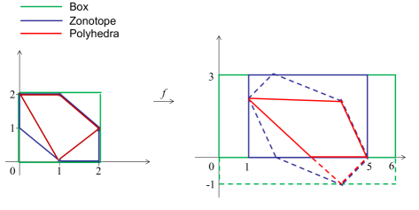
Figure 2: An illustration of Example 1 and Example 2, where on the right the dashed lines gives the abstraction region before the $\mathrm{ReLU}$ operation and the full lines gives the final abstraction $f^{\sharp}(X^{\sharp})$.

3 Symbolic Propagation for Abstract Interpretation based DNN Verification

In this section, we first describe how to use abstract interpretation to verify DNNs. Then we present a symbolic propagation method to enhance its precision.

3.1 Abstract interpretation based DNN verification

3.1.1 The DNN verification problem

The problem of verifying DNNs over a property can be stated formally as follows.

Definition 2

Given a function $f:\mathbb{R}^{m}\to\mathbb{R}^{n}$ which expresses a DNN, a set of the inputs $X_{0}\subseteq\mathbb{R}^{m}$, and a property $C\subseteq\mathbb{R}^{n}$, verifying the property is to determine whether $f(X_{0})\subseteq C$ holds, where $f(X_{0})=\{f(\bar{x})~{}|~{}\bar{x}\in X_{0}\}$.

Local robustness property can be obtained by letting $X_{0}$ be a robustness region and $C$ be $C_{l}:=\{\bar{y}\in\mathbb{R}^{n}\mid\arg\max_{1\leq i\leq n}y_{i}=l\}$. where $y$ denotes an output vector and $l$ denotes a label.

A common way of defining robustness region is with norm distance. We use $\|\bar{x}-\bar{x}_{0}\|_{p}$ with $p\in[1,\infty]$ to denote the $L_{p}$ norm distance between two vectors $\bar{x}$ and $\bar{x}_{0}$. In this paper, we use $L_{\infty}$ norm defined as follows.

$$\|\bar{x}\|_{\infty}=\max_{1\leq i\leq n}|x_{i}|.$$

Given an input $\bar{x}_{0}\in\mathbb{R}^{m}$ and a perturbation tolerance $\delta>0$, a local robustness region $X_{0}$ can be defined as $B(\bar{x}_{0},\delta):=\{\bar{x}\mid\|\bar{x}-\bar{x}_{0}\|_{p}\leq\delta\}$.

3.1.2 Verifying DNNs via abstract interpretation

Under the framework of abstract interpretation, to conduct verification of DNNs, we first need to choose an abstract domain ${\cal A}$. Then we represent the set of inputs of a DNN as an abstract element (value) $X^{\sharp}_{0}$ in ${\cal A}$. After that, we pass it through the DNN layers by applying abstract transformers of the abstract domain. Recall that $N$ is the number of layers in a DNN and ${m_{k}}$ is the number of nodes in the $k$-th layer. Let $f_{k}$ (where $1\leq k<N$) be the layer function mapping from ${\mathbb{R}}^{m_{k-1}}$ to ${\mathbb{R}}^{m_{k}}$. We can lift $f_{k}$ to $T_{f_{k}}:{\cal P}({\mathbb{R}}^{m_{k-1}})\rightarrow{\cal P}({\mathbb{R}}^{m_{k}})$ such that $T_{f_{k}}(X)=\{f_{k}(\bar{x})\mid\bar{x}\in X\}$.

Definition 3

An abstract transformer $T_{f_{k}}^{\sharp}$ is a function mapping an abstract element $X^{\sharp}_{k-1}$ in the abstract domain ${\cal A}$ to another abstract element ${X^{\sharp}}_{k}$. Moreover, $T_{f_{k}}^{\sharp}$ is sound if $T_{f_{k}}\circ\gamma\subseteq\gamma\circ T_{f_{k}}^{\sharp}$.

Intuitively, a sound abstract transformer $T_{f_{k}}^{\sharp}$ maintains a sound relation between the abstract post-state and the abstract pre-state of a transformer in DNN (such as linear transformation, ReLU operation, etc.).

Let $X_{k}=f_{k}(...(f_{1}(X_{0})))$ be the exact set of resulting vectors in $\mathbb{R}^{m_{k}}$ (i.e., the $k$-th layer) computed over the concrete inputs $X_{0}$, and $X{{}^{\sharp}}_{k}=T_{f_{k}}{{}^{\sharp}}(...(T_{f_{1}}{{}^{\sharp}}(X{{}^{\sharp}}_{0})))$ be the corresponding abstract value of the $k$-th layer when using an abstract domain ${\cal A}$. Note that $X_{0}\subseteq\gamma({X^{\sharp}}_{0})$. We have the following conclusion.

Proposition 1

If $X_{k-1}\subseteq\gamma({X^{\sharp}}_{k-1})$, then we have $X_{k}\subseteq\gamma({X^{\sharp}}_{k})=\gamma\circ T_{f_{k}}^{\sharp}({{X^{\sharp}}}_{k-1})$.

Therefore, when performing abstract interpretation over the transformations in a DNN, the abstract pre-state ${X^{\sharp}}_{k-1}$ is transformed into abstract post-state ${X^{\sharp}}_{k}$ by applying the abstract transformer $T_{f_{k}}^{\sharp}$ which is built on top of an abstract domain. This procedure starts from $k=1$ and continues until reaching the output layer (and getting ${X^{\sharp}}_{N-1}$). Finally, we use ${X^{\sharp}}_{N-1}$ to check the property $C$ as follows:

$$\gamma({X^{\sharp}}_{N-1})\subseteq C.$$ (1)

The following theorem states that this verification procedure based on abstract interpretation is sound for the DNN verification problem.

Theorem 3.1

If Equation (1) holds, then $f(X_{0})\subseteq C$.

It’s not hard to see that the other direction does not necessarily hold due to the potential incompleteness caused by the over-approximation made in both the abstract elements and the abstract transformers $T_{f_{k}}^{\sharp}$ in an abstract domain.

Example 2

Suppose that $\bar{x}$ takes the value in $X$ given in Example 1, and we consider the transformation $f(\bar{x})=\mathrm{ReLU}\left(\begin{pmatrix}1&2\\ 1&-1\end{pmatrix}\bar{x}+\begin{pmatrix}0\\ 1\end{pmatrix}\right)$. Now we use the three abstract domains to calculate the resulting abstraction $f^{\sharp}(X^{\sharp})$

• Box. The abstraction after the affine transformation is $[0,6]\times[-1,3]$, and thus the final result is $[0,6]\times[0,3]$.

• Zonotope. After the affine transformation, the zonotope abstraction can be obtained straightforward:

  $$\left\{y_{1}=3+\frac{1}{2}\epsilon_{1}+\epsilon_{2}-\frac{1}{2}\epsilon_{3},\enspace y_{2}=1-\epsilon_{1}-\frac{1}{2}\epsilon_{2}-\frac{1}{2}\epsilon_{3}\mid\epsilon_{1},\epsilon_{2},\epsilon_{3}\in[-1,1]\right\}.$$

  The first dimension $y_{1}$ is definitely positive, so it remains the same after the $\mathrm{ReLU}$ operation. The second dimension $y_{2}$ can be either negative or non-negative, so its abstraction after $\mathrm{ReLU}$ will become a box which only preserves the range in the non-negative part, i.e. $[0,3]$, so the final abstraction is

  $$\left\{y_{1}=3+\frac{1}{2}\epsilon_{1}+\epsilon_{2}-\frac{1}{2}\epsilon_{3},\enspace y_{2}=\frac{3}{2}+\frac{3}{2}\eta_{1}\mid\epsilon_{1},\epsilon_{2},\epsilon_{3},\eta_{1}\in[-1,1]\right\},$$

  whose concretization is $[1,5]\times[0,3]$.

• Polyhedra. It is easy to obtain the polyhedron before $P_{1}=\mathrm{ReLU}$ $\{y_{2}\leq 2,y_{2}\geq-y_{1}+3,y_{2}\geq y_{1}-5,y_{2}\leq-2y_{1}+10\}$. Similarly, the first dimension is definitely positive, and the second dimension can be either negative or non-negative, so the resulting abstraction is $(P_{1}\wedge(y_{2}\geq 0))\vee(P_{1}\wedge(y_{2}=0))$, i.e. $\{y_{2}\leq 2,y_{2}\geq-y_{1}+3,y_{2}\geq 0,y_{2}\leq-2y_{1}+10\}$.

Fig. 2 (the right part) gives an illustration for the abstract interpretation with the three abstract domains in this example.

The abstract value computed via abstract interpretation can be directly used to verify properties. Take the local robustness property, which expresses an invariance on the classification of $f$ over a region $B(\bar{x}_{0},\delta)$, as an example. Let $l_{i}(\bar{x})$ be the confidence of $\bar{x}$ being labeled as $i$, and $l(\bar{x})=\mathrm{argmax}_{i}l_{i}(\bar{x})$ be the label. It has been shown in [30, 25] that DNNs are Lipschitz continuous. Therefore, when $\delta$ is small, we have that $|l_{i}(\bar{x})-l_{i}(\bar{x}_{0})|$ is also small for all labels $i$. That is, if $l_{i}(\bar{x}_{0})$ is significantly greater than $l_{j}(\bar{x}_{0})$ for $j\neq i$, it is highly likely that $l_{i}(\bar{x})$ is also significantly greater than $l_{j}(\bar{x})$. It is not hard to see that the more precise the relations among $l_{i}(\bar{x}_{0}),l_{i}(\bar{x}),l_{j}(\bar{x}_{0}),l_{j}(\bar{x})$ computed via abstract interpretation, the more likely we can prove the robustness. Based on this reason, this paper aims to derive techniques to enhance the precision of abstract interpretation such that it can prove some more properties that cannot be proven by the original abstract interpretation.

3.2 Symbolic propagation for DNN verification

Symbolic propagation can ensure soundness while providing more precise results. In [31], a technique called symbolic interval propagation is present and we extend it to our abstraction interpretation framework so that it works on all abstract domains. First, we use the following example to show that using only abstract transformations in an abstract domain may lead to precision loss, while using symbolic propagation could enhance the precision.

Example 3

Assume that we have a two-dimensional input $(x_{1},x_{2})\in[0,1]\times[0,1]$ and a few transformations $y_{1}:=x_{1}+x_{2}$, $y_{2}:=x_{1}-x_{2}$, and $z:=y_{1}+y_{2}$. Suppose we use the Box abstract domain to analyze the transformations.

• When using only the Box abstract domain, we have $y_{1}\in[0,2]$, $y_{2}\in[-1,1]$, and thus $z\in[-1,3]$ (i.e., $[0,2]+[-1,1]$).

• By symbolic propagation, we record $y_{1}=x_{1}+x_{2}$ and $y_{2}=x_{1}-x_{2}$ on the neurons $y_{1}$ and $y_{2}$ respectively, and then get $z=2x_{1}\in[0,2]$. This result is more precise than that given by using only the Box abstract domain.

Non-relational (e.g., intervals) and weakly-relational abstract domains (e.g., zones, octagons, zonotopes, etc.)[19] may lose precision on the application of the transformations from DNNs. The transformations include affine transformations, ReLU, and max pooling operations. Moreover, it is often the case for weakly-relational abstract domains that the composition of the optimal abstract transformers of individual statements in a sequence does not result in the optimal abstract transformer for the whole sequence, which has been shown in Example 3 when using only the Box abstract domain. A choice to precisely handle general linear transformations is to use the Polyhedra abstract domain which uses a conjunction of linear constraints as domain representation. However, the Polyhedra domain has the worst-case exponential space and time complexity when handling the ReLU operation (via the join operation in the abstract domain). As a consequence, DNN verification with the Polyhedra domain is impractical for large scale DNNs, which has been also confirmed in [10].

In this paper, we leverage symbolic propagation technique to enhance the precision for abstract interpretation based DNN verification. The insight behind is that affine transformations account for a large portion of the transformations in a DNN. Furthermore, when we verify properties such as robustness, the activation of a neuron can often be deterministic for inputs around an input with small perturbation. Hence, there should be a large number of linear equality relations that can be derived from the composition of a sequence of linear transformations via symbolic propagation. And we can use such linear equality relations to improve the precision of the results given by abstract domains. In Section 6, our experimental results confirm that, when the perturbation tolerance $\delta$ is small, there is a significant proportion of neurons whose ReLU activations are consistent.

First, given $X_{0}$, a $\mathrm{ReLU}$ neuron $y:=\mathrm{ReLU}(\sum_{i=1}^{n}w_{i}x_{i}$ $+b)$ can be classified into one of the following 3 categories (according to its range information): (1) definitely-activated, if the range of $\sum_{i=1}^{n}w_{i}x_{i}+b$ is a subset of $[0,\infty)$, (2) definitely-deactivated, if the range of $\sum_{i=1}^{n}w_{i}x_{i}+b$ is a subset of $(-\infty,0]$, and (3) uncertain, otherwise.

Now we detail our symbolic propagation technique. We first introduce a symbolic variable $s_{i}$ for each node $i$ in the input layer, to denote the initial value of that node. For a $\mathrm{ReLU}$ neuron $d:=\mathrm{ReLU}(\sum_{i=1}^{n}w_{i}c_{i}+b)$ where $c_{i}$ is a symbolic variable, we make use of the resulting abstract value of abstract domain at this node to determine whether the value of this node is definitely greater than 0 or definitely less than 0. If it is a definitely-activated neuron, we record for this neuron the linear combination $\sum_{i=1}^{n}w_{i}c_{i}+b$ as its symbolic representation (i.e., the value of symbolic propagation). If it is a definitely-deactivated neuron, we record for this neuron the value $0$ as its symbolic representation. Otherwise, we cannot have a linear combination as the symbolic representation and thus a fresh symbolic variable $s_{d}$ is introduced to denote the output of this $\mathrm{ReLU}$ neuron. We also record the bounds for $s_{d}$, such that the lower bound for $s_{d}$ is set to 0 (since the output of a $\mathrm{ReLU}$ neuron is always non-negative) and the upper bound keeps the one obtained by abstract interpretation.

To formalize the algorithm for ReLU node, we first define the abstract states in the analysis and three transfer functions for linear assignments, condition tests and joins respectively. An abstract state in our analysis is composed of an abstract element for a numeric domain (e.g., Box) $\mathbf{n}^{\#}\in\mathbf{N}^{\#}$, a set of free symbolic variables $\mathbf{C}$ (those not equal to any linear expressions), a set of constrained symbolic variables $\mathbf{S}$ (those equal to a certain linear expression), and a map from constrained symbolic variables to linear expressions $\xi::=\mathbf{S}\Rightarrow\{\sum_{i=1}^{n}a_{i}x_{i}+b\mid x_{i}\in\mathbf{C}\}$. Note that we only allow free variables in the linear expressions in $\xi$. In the beginning, all input variables are taken as free symbolic variables. In Algorithm 1, we show the transfer functions for linear assignments $[\kern-1.49994pt[y:=\sum_{i=1}^{n}w_{i}x_{i}+b]\kern-1.49994pt]^{\sharp}$ which over-approximates the behaviors of $y:=\sum_{i=1}^{n}w_{i}x_{i}+b$. If $n>0$ (i.e., the right value expression is not a constant), variable $y$ is added to the constrained variable set $\mathbf{S}$. All constrained variables in $\mathbf{expr}=\sum_{i=1}^{n}w_{i}x_{i}+b$ are replaced by their corresponding expressions in $\xi$, and the map from $y$ to the new $\mathbf{expr}$ is recorded in $\xi$. Abstract numeric element $\mathbf{n}^{\#}$ is updated by the transfer function for assignments in the numeric domain $[\kern-1.49994pt[y:=\mathbf{expr}]\kern-1.49994pt]^{\sharp}_{\mathbf{N}^{\#}}$. If $n\leq 0$, the right-value expression is a constant, then $y$ is added to $\mathbf{C}$, and is removed from $\mathbf{S}$ and $\xi$.

The abstract transfer function for condition test is defined as

$$[\kern-1.49994pt[\mathbf{expr}\leq 0]\kern-1.49994pt]^{\sharp}(\mathbf{n}^{\#},\mathbf{C},\mathbf{S},\xi)::=([\kern-1.49994pt[\mathbf{expr}\leq 0]\kern-1.49994pt]^{\sharp}_{\mathbf{N}^{\#}}(\mathbf{n}^{\#}),\mathbf{C},\mathbf{S},\xi),$$

which only updates the abstract element $\mathbf{n}^{\#}$ by the transfer function in the numeric domain $\mathbf{N}^{\#}$.

1

Input: abstract numeric element $\mathbf{n}^{\#}\in\mathbf{N}^{\#}$, free variables $\mathbf{C}$, constrained variables $\mathbf{S}$, symbolic map $\xi$

2

3$\mathbf{expr}\leftarrow\sum_{i=1}^{n}w_{i}x_{i}+b$

4When the right value expression is not a constant

5if $n>0$ then

6       for $i\in[1,n]$ do

7             if $x_{i}\in\mathbf{S}$ then

8                   $\mathbf{expr}=\mathbf{expr}_{|x_{i}\leftarrow\xi(x_{i})}$

9             end if

10            

11       end for

12      $\xi=\xi\cup\{y\mapsto\mathbf{expr}\}$ $\mathbf{S}=\mathbf{S}\cup\{y\}$ $\mathbf{C}=\mathbf{C}/\{y\}$ $\mathbf{n}^{\#}=[\kern-1.49994pt[y:=\mathbf{expr}]\kern-1.49994pt]^{\sharp}_{\mathbf{N}^{\#}}$

13else

14       $\xi=\xi/(y\mapsto*)$ $\mathbf{C}=\mathbf{C}\cup\{y\}$ $\mathbf{S}=\mathbf{S}/\{y\}$ $\mathbf{n}^{\#}=[\kern-1.49994pt[y:=\mathbf{expr}]\kern-1.49994pt]^{\sharp}_{\mathbf{N}^{\#}}$

15 end if

return $(\mathbf{n}^{\#},\mathbf{C},\mathbf{S},\xi)$

Algorithm 1 Transfer function for linear assignments $[\kern-1.49994pt[y:=\sum_{i=1}^{n}w_{i}x_{i}+b]\kern-1.49994pt]^{\sharp}$

The join algorithm in our analysis is defined in Algorithm 2. Only the constrained variables arising in both input $\mathbf{S}_{0}$ and $\mathbf{S}_{1}$ are with the same corresponding linear expressions are taken as constrained variables. The abstract element in the result is obtained by applying the join operator in the numeric domain $\sqcup_{\mathbf{N}^{\#}}$.

The transfer function for a ReLU node is defined as

$$[\kern-1.49994pt[y:=\mathrm{ReLU}(\sum_{i=1}^{n}w_{i}x_{i}+b)]\kern-1.49994pt]^{\sharp}(\mathbf{n}^{\#},\mathbf{C},\mathbf{S},\xi)::=\mathbf{join}([\kern-1.49994pt[y>0]\kern-1.49994pt]^{\sharp}(\psi),[\kern-1.49994pt[y:=0]\kern-1.49994pt]^{\sharp}([\kern-1.49994pt[y<0]\kern-1.49994pt]^{\sharp})(\psi)),$$

where $\psi=[\kern-1.49994pt[y:=\sum_{i=1}^{n}w_{i}x_{i}+b]\kern-1.49994pt]^{\sharp}(\mathbf{n}^{\#},\mathbf{C},\mathbf{S},\xi)$.

Input: $(\mathbf{n}^{\#}_{0},\mathbf{C}_{0},\mathbf{S}_{0},\xi_{0})$ and $(\mathbf{n}^{\#}_{1},\mathbf{C}_{1},\mathbf{S}_{1},\xi_{1})$

1

2$\mathbf{n}^{\#}=\mathbf{n}^{\#}_{0}\sqcup_{\mathbf{N}^{\#}}\mathbf{n}^{\#}_{1}$

3$\xi=\xi_{0}\cap\xi_{1}$

4$\mathbf{S}=\{x\mid\exists\mathbf{expr},x\rightarrow\mathbf{expr}\in\xi\}$

5$\mathbf{C}=\mathbf{C}_{0}\cup(\mathbf{S}_{0}/\mathbf{S})$

return $(\mathbf{n}^{\#},\mathbf{C},\mathbf{S},\xi)$

Algorithm 2 Join algorithm $\mathbf{join}$

For a max pooling node $d:=\max_{1\leq i\leq k}c_{i}$, if there exists some $c_{j}$ whose lower bound is larger than the upper bound of $c_{i}$ for all $i\neq j$, we set $c_{j}$ as the symbolic representation for $d$. Otherwise, we introduce a fresh symbolic variable $s_{d}$ for $d$ and record its bounds wherein its lower (upper) bound is the maximum of the lower (upper) bounds of $c_{i}$’s. Note that the lower (upper) bound of each $c_{i}$ can be derived from the abstract value for this neuron given by abstract domain.

The algorithm for max-pooling layer can be defined with the three aforementioned transfer functions as follows:

$$\begin{array}[]{c}\mathbf{join}(\phi_{1},\mathbf{join}(\phi_{2},\ldots,\mathbf{join}(\phi_{k-1},\phi_{k}))),\\ \text{where}\quad\phi_{i}=[\kern-1.49994pt[d:=c_{i}]\kern-1.49994pt]^{\sharp}[\kern-1.49994pt[c_{i}\geq c_{1}]\kern-1.49994pt]^{\sharp}\ldots[\kern-1.49994pt[c_{i}\geq c_{k}]\kern-1.49994pt]^{\sharp}(\mathbf{n}^{\#},\mathbf{C},\mathbf{S},\xi)\end{array}$$

Example 4

For the DNN shown in Figure 3(a), there are two input nodes denoted by symbolic variables $x$ and $y$, two hidden nodes, and one output node. The initial ranges of the input symbolic variables $x$ and $y$ are given, i.e., $[4,6]$ and $[3,4]$ respectively. The weights are labeled on the edges. It is not hard to see that, when using the Interval abstract domain, (the inputs of) the two hidden nodes have bounds $[17,24]$ and $[0,3]$ respectively. For the hidden node with $[17,24]$, we know that this ReLU node is definitely activated, and thus we use symbolic propagation to get a symbolic expression $2x+3y$ to symbolically represent the output value of this node. Similarly, for the hidden node with $[0,3]$, we get a symbolic expression $x-y$. Then for the output node, symbolic propagation results in $x+4y$, which implies that the output range of the whole DNN is $[16,22]$. If we use only the Interval abstract domain without symbolic propagation, we will get the output range $[14,24]$, which is less precise than $[16,22]$.

For the DNN shown in Figure 3(b), we change the initial range of the input variable $y$ to be $[4.5,5]$. For the hidden ReLU node with $[-1,1.5]$, it is neither definitely activated nor definitely deactivated, and thus we introduce a fresh symbolic variable $s$ to denote the output of this node, and set its bound to $[0,1.5]$. For the output node, symbolic propagation results in $2x+3y-s$, which implies that the output range of the whole DNN is $[20,27]$.

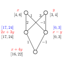
(a)                                         (b)

Figure 3: An illustrative example of symbolic propagation

For a definitely-activated neuron, we utilize its symbolic representation to enhance the precision of abstract domains. We add the linear constraint $d==\sum_{i=1}^{n}w_{i}c_{i}+b$ into the abstract value at (the input of) this node, via the meet operation (which is used to deal with conditional test in a program) in the abstract domain [3]. If the precision of the abstract value for the current neuron is improved, we may find more definitely-activated neurons in the subsequent layers. In other words, the analysis based on abstract domain and our symbolic propagation mutually improves the precision of each other on-the-fly.

After obtaining symbolic representation for all the neurons in a layer $k$, the computation proceeds to layer $k+1$. The computation terminates after completing the computation for the output layer. All symbolic representations in the output layer are evaluated to obtain value bounds.

The following theorem shows some results on precision of our symbolic propagation technique.

Theorem 3.2

(1) For an FNN $f:\mathbb{R}^{m}\to\mathbb{R}^{n}$ and a box region $X\subseteq\mathbb{R}^{m}$, the Box abstract domain with symbolic propagation can give a more precise abstraction for $f(X)$ than the Zonotope abstract domain without symbolic propagation.

(2) For an FNN $f:\mathbb{R}^{m}\to\mathbb{R}^{n}$ and a box region $X\subseteq\mathbb{R}^{m}$, the Box abstract domain with symbolic propagation and the Zonotope abstract domain with symbolic propagation gives the same abstraction for $f(X)$.

(3) There exists a CNN $g:\mathbb{R}^{m}\to\mathbb{R}^{n}$ and a box region $X\subseteq\mathbb{R}^{m}$ s.t. the Zonotope abstract domain with symbolic propagation give a more precise abstraction for $g(X)$ than the Box abstract domain with symbolic propagation.

Proof

(1) Since an FNN only contains fully connected layers, we just need to prove that, Box with symbolic propagation (i.e., BoxSymb) is always more precise than Zonotope in the transformations on each RELU neuron $y:=\mathrm{ReLU}(\sum_{i=1}^{n}w_{i}x_{i}$ $+b)$. Assume that before the transformation, BoxSymb is more precise or as precise as Zonotope. Since the input is a Box region, the assumption is valid in the beginning. Then we consider three cases: (a) in BoxSymb, the sign of $\sum_{i=1}^{n}w_{i}x_{i}+b$ is uncertain, then it must also be uncertain in Zonotope. In both domains, a constant interval with upper bound computed by $\sum_{i=1}^{n}w_{i}x_{i}+b$ and lower bound as 0 is assigned to $y$ (this can be inferred from our aforementioned algorithms and [11]). With our assumption, the upper bound computed by BoxSymb is more precise than that in Zonotope; (b) in BoxSymb, the sign of $\sum_{i=1}^{n}w_{i}x_{i}+b$ is always positive, then it must be always positive or uncertain in Zonotope. In the former condition, BoxSymb is more precise because it loses no precision, while Zonotope can lose precision because of its limited expressiveness. In the later condition, BoxSymb is more precise obviously; (c) in BoxSymb, the sign of $\sum_{i=1}^{n}w_{i}x_{i}+b$ is always negative, then it must be always negative or uncertain in Zonotope. Similar to case (b), BoxSymb is also more precise in this case.

(2) Assume that before each transformation on a ReLU neuron $y:=\mathrm{ReLU}(\sum_{i=1}^{n}w_{i}x_{i}$ $+b)$, BoxSymb and ZonoSymb (Zonotope with symbolic propagation) are with same precision. This assumption is also valid when the input is a Box region. Then the evaluation of $\sum_{i=1}^{n}w_{i}x_{i}+b$ is same in BoxSymb and ZonoSymb, thus in the three cases:(a) the sign of $\sum_{i=1}^{n}w_{i}x_{i}+b$ is uncertain, they both compute a same constant interval for $y$; (b) and (c) $\sum_{i=1}^{n}w_{i}x_{i}+b$ is always positive or negative, they both lose no precision.

(3) It is easy to know that, ZonoSymb is more precise or as precise as BoxSymb in all transformations. In CNN, with Max-Pooling layer, we just need to give an example that ZonoSymb can be more precise. Let the Zonotope $X^{\prime}=\{x_{1}=2+\epsilon_{1}+\epsilon_{2},\enspace x_{2}=2+\epsilon_{1}-\epsilon_{2}\mid\epsilon_{1},\epsilon_{2}\in[-1,1]\}$ and the max pooling node $y=\max\{x_{1},x_{2}\}$. Obviously $X^{\prime}$ can be obtained through a linear transformation on some box region $X$. With Box with symbolic propagation, the abstraction of $y$ is $[0,4]$, while Zonotope with symbolic propagation gives the abstraction is $[1,4]$.

Thm 3.2 gives us some insights: Symbolic propagation technique has a very strong power (even stronger than Zonotope) in dealing with ReLU nodes, while Zonotope gives a more precise abstraction on max pooling nodes. It also provides a useful instruction: When we work with FNNs with the input range being a box, we should use Box with symbolic propagation rather than Zonotope with symbolic propagation since it does not improve the precision but takes more time. Results in Thm 3.2 will also be illustrated in our experiments.

4 Abstract Interpretation as an Accelerator for SMT-based DNN Verification

In this section we briefly recall DNN verification based on SMT solvers, and then describe how to utilize the results by abstract interpretation with our symbolic propagation to improve its performance.

4.1 SMT based DNN verification

In [15, 8], two SMT solvers Reluplex and Planet were presented to verify DNNs. Typically an SMT solver is the combination of a SAT solver with the specialized decision procedures for other theories. The verification of DNNs uses linear arithmetic over real numbers, in which an atom may have the form of $\sum_{i=1}^{n}w_{i}x_{i}\leq b$, where $w_{i}$ and $b$ are real numbers. Both Reluplex and Planet use the DPLL algorithm to split cases and rule out conflict clauses. They are different in dealing with the intersection. For Reluplex, it inherits rules from the Simplex algorithm and adds a few rules dedicated to $\mathrm{ReLU}$ operation. Through the classical pivot operation, it searches for a solution to the linear constraints, and then apply the rules for $\mathrm{ReLU}$ to ensure the $\mathrm{ReLU}$ relation for every node. Differently, Planet uses linear approximation to over-approximate the DNN, and manage the conditions of $\mathrm{ReLU}$ and max pooling nodes with logic formulas.

4.2 Abstract interpretation with symbolic propagation as an accelerator

SMT-based DNN verification approaches are often not efficient, e.g., relying on case splitting for ReLU operation. In the worst case, case splitting is needed for each ReLU operation in a DNN, which leads to an exponential blow-up. In particular, when analyzing large-scale DNNs, SMT-based DNN verification approaches may suffer from the scalability problem and account time out, which is also confirmed experimentally in [10].

In this paper, we utilize the results of abstract interpretation (with symbolic propagation) to accelerate SMT-based DNN verification approaches. More specifically, we use the bound information of each ReLU node (obtained by abstract interpretation) to reduce the number of case-splitting, and thus accelerate SMT-based DNN verification. For example, on a neuron $d:=\mathrm{ReLU}(\sum_{i=1}^{n}w_{i}c_{i}+b)$, if we know that this node is a definitely-activated node according to the bounds given by abstract interpretation, we only consider the case $d:=\sum_{i=1}^{n}w_{i}c_{i}+b$ and thus no split is applied. We remark that, this does not compromise the precision of SMT-based DNN verification while improving their efficiency.

5 Discussion

In this section, we discuss the soundness guarantee of our approach. Soundness is an essential property of formal verification.

Abstract interpretation is known for its soundness guarantee for analysis and verification [19], since it conducts over-approximation to enclose all the possible behaviors of the original system. Computing over-approximations for a DNN is thus our soundness guarantee in this paper. As shown in Theorem 3.1, if the results of abstract interpretation show that the property $C$ holds (i.e., $\gamma({X^{\sharp}}_{N})\subseteq C$ in Equation 1), then the property also holds for the set of actual executions of the DNN (i.e., $f(X_{0})\subseteq C$). If the results of abstract interpretation can not prove that the property $C$ holds, however, the verification is inconclusive. In this case, the results of the chosen abstract domain are not precise enough to prove the property, and thus more powerful abstract domains are needed. Moreover, our symbolic propagation also preserves soundness, since it uses symbolic substitution to compute the composition of linear transformations.

On the other hand, many existing DNN verification tools do not guarantee soundness. For example, Reluplex [15] (using GLPK), Planet [8] (using GLPK), and Sherlock [4] (using Gurobi) all rely on the floating point implementation of linear programming solvers, which is unsound. Actually, most state-of-the-art linear programming solvers use floating-point arithmetic and only give approximate solutions which may not be the actual optimum solution or may even lie outside the feasible space [21]. It may happen that a linear programming solver implemented via floating point arithmetic wrongly claims that a feasible linear system is infeasible or the other way round. In fact, [4] reports several false positive results in Reluplex, and mentions that this comes from unsound floating point implementation.

6 Experimental Evaluation

We present the design and results of our experiments.

6.1 Experimental setup

Implementation. c is the first to utilize abstract interpretation to verify DNNs, and has implemented all the transformers mentioned in Section 3.1. Since the implementation of AI² is not available, we have re-implemented these transformers and refer to them as AI²-r. We then implemented our symbolic propagation technique based on AI²-r and use AI²-r as the baseline comparison in the experiments. Both implementations use general frameworks and thus can run on various abstract domains. In this paper, we chose Box (from Apron ), T-Zonotope (Zonotope from Apron 1) and E-Zonotope (Elina Zonotope with the join operator ) as the underlying domains.

Datasets and DNNs. We use MNIST [17] and ACAS Xu [13, 9] as the datasets in our experiments. MNIST contains $60,000$ $28\times 28$ grayscale handwritten digits. We can train DNNs to classify the pictures by the written digits on them. The ACAS Xu system is aimed to avoid airborne collisions and it uses an observation table to make decisions for the aircraft. In [14], the observation table can be realized by training a DNN instead of storing it.

On MNIST, we train seven FNNs and two CNNs. The seven FNNs are of the size $3\times 20$, $6\times 20$, $3\times 50$, $3\times 100$, $6\times 100$, and $9\times 200$, where $m\times n$ refers to $m$ hidden layers with $n$ neurons in each hidden layer. The CNN1 consists of $2$ convolutional, $1$ max-pooling, $2$ convolutional, $1$ max-pooling, and $3$ fully connected layers in sequence, for a total of 12,412 neurons. The CNN2 has $4$ convolutional and $3$ fully connected layers (89572 neurons). On ACAS Xu, we use the same networks as those in [15].

Properties. We consider the local robustness property with respect to the input region defined as follows:

$$X_{\bar{x},\delta}=\{\bar{x}^{\prime}\in\mathbb{R}^{m}\mid\forall i.1-\delta\leq x_{i}\leq x_{i}^{\prime}\leq 1\vee x_{i}=x_{i}^{\prime}\}.$$

In the experiments, the optional robustness bounds are $0.1,0.2,0.3,0.4,0.5,0.6$. All the experiments are conducted on an openSUSE Leap 15.0 machine with Intel i7 CPU@3.60GHz and 16GB memory.

6.2 Experimental Results

	AI2-r		Symb			Planet
	TZono	EZono	Box	TZono	EZono
FNN1	28.23348%	28.02098%	9.69327%	9.69327%	9.69327%	7.05553%
FNN2	24.16382%	22.13319%	1.76704%	1.76704%	1.76704%	0.89089%
FNN3	26.66453%	26.30852%	6.88656%	6.88656%	6.88656%	4.51223%
FNN4	28.47243%	28.33535%	5.13645%	5.13645%	5.13645%	2.71537%
FNN5	35.61163%	35.27187%	3.34578%	3.34578%	3.34578%	0.14836%
FNN6	38.71020%	38.57376%	7.12480%	7.12480%	7.12480%	1.94230%
FNN7	41.76517%	41.59382%	5.52267%	5.52267%	5.52267%	1h TIMEOUT
CNN1	24.19607%	24.13725%	21.78279%	7.58917%	7.56223%	8h TIMEOUT
CNN2	OOM	OOM	1.09146%	OOM	OOM	8h TIMEOUT

(a) Bound proportions (smaller is better) of different abstract interpretation approaches with the robustness bound $\delta\in\{0.1,0.2,0.3,0.4,0.5,0.6\}$, and the fixed input pictures 767, 1955, and 2090;

	AI2-r						Symb						Planet
	Box		TZono		EZono		Box		TZono		EZono
FNN1	11.168	0.2	13.482	0.5	44.05	0.5	12.935	0.6	17.144	0.6	45.88	0.6	20.179	0.6
FNN2	12.559	0	16.636	0.2	50.59	0.2	15.075	0.5	22.333	0.5	49.92	0.5	35.84	0.6
FNN3	12.699	0.2	18.748	0.3	49.812	0.3	19.042	0.6	28.128	0.6	54.77	0.6	76.106	0.6
FNN4	15.583	0.1	29.495	0.3	58.892	0.3	37.716	0.6	56.47	0.6	76.00	0.6	351.139	0.6
FNN5	28.963	0	81.49	0.2	149.791	0.2	90.268	0.4	154.222	0.4	173.263	0.4	1297.485	0.6
FNN6	62.766	0	398.565	0.1	538.076	0.1	323.328	0.3	650.629	0.3	745.454	0.3	15823.208	0.3
FNN7	111.955	0	1674.465	0	1627.72	0	642.978	0.3	1524.975	0.3	1489.604	0.3	1h TIMEOUT
CNN1	2340.828	0	6717.57	0.2	94504.195	0.2	5124.681	0.2	8584.555	0.3	45452.102	0.3	8h TIMEOUT
CNN2	41292.291	0	OOM	0	OOM	0	105850.271	0.3	OOM	0	OOM	0	8h TIMEOUT

(b) The time (in second) and the maximum robustness bound $\delta$ which can be verified through the abstract interpretation technique and the planet bound, with optional $\delta\in\{0.1,0.2,0.3,0.4,0.5,0.6\}$ and the fixed input picture 2090;

	AI2-r			Symb			Planet
	Box	TZono	EZono	Box	TZono	EZono
FNN1(60)	57  44  34	59  52  38	59  52  38	59  53  44	59 53 44	59 53 44	59 56 55
FNN2(120)	103  59  38	118  109  66	118  111  66	118  113  107	118 113 107	118 113 107	119 114 110
FNN3(150)	136  93  66	141  127  85	141  127  85	143  133  110	143 133 110	143 133 110	146 142 135
FNN4(300)	250  144  105	294  209  130	294  209  130	295  254  182	295 254 182	295 254 182	296 276 254
FNN5(600)	289  160  106	513  200  125	513  200  125	589  510  236	589 510 236	589 510 236	593 558 493
FNN6(1200)	472  247  181	782  339  195	782  339  195	1176  790  250	1176 790 250	1176 790 250	1189 1089 772
FNN7(1800)	469  271  177	770  350  200	775  350  200	1773  741  263	1773 741 263	1773 741 263	1h TIMEOUT
CNN1(12412)	12226  11788  11280	12371  12119  11786	12371  12122  11786	12373  12094  11659	12376 12193 11877	12376 12196  11877	8h TIMEOUT
CNN2(89572)	85793  77241  70212	OOM	OOM	89190  86910  81442	OOM	OOM	8h TIMEOUT

(c) The number of hidden $\mathrm{ReLU}$ neurons whose behavior can be decided with the bounds our abstract interpretation technique and Planet provide, with optional robustness bound $\delta\in\{0.1,0.4,0.6\}$ and the fixed input picture 767.

Table 1: Experimental results of abstract interpretation for MNIST DNNs with different approaches

We compare seven approaches: AI²-r  with Box, T-Zonotope and E-zonotope as underlying domains and Symb (i.e., our enhanced abstract interpretation with symbolic propagation) with Box, T-Zonotope and E-zonotope as underlying domains, and Planet [8], which serves as the benchmark verification approach (for its ability to compute bounds).

Improvement on Bounds

To see the improvement on bounds, we compare the output ranges of the above seven approaches on different inputs $\bar{x}$ and different tolerances $\delta$. Table 1(a) reports the results on three inputs $\bar{x}$ (No.767, No.1955 and No.2090 in the MNIST training dataset) and six tolerances $\delta\in\{0.1,0.2,0.3,0.4,0.5,0.6\}$. In all our experiments, we set TIMEOUT as one hour for each FNN and eight hours for each CNN for a single run with an input, and a tolerance $\delta$. In the table, TZono and EZono are shorts for T-Zonotope and E-Zonotope.

For each running we get a gap with an upper and lower bound for each neuron. Here we define the the bound proportion to statistically describe how precise the range an approach gives. Basically given an approach (like Symb with Box domain), the bound proportion of this approach is the average of the ratio of the gap length of the neurons on the output layer and that obtained using AI²-r with Box. Naturally AI²-r  with Box always has the bound proportion $1$, and the smaller the bound proportion is, the more precise the ranges the approach gives are.

In Table 1(a), every entry is the average bound proportion over three different inputs and six different tolerances. OOM stands for out-of-memory, 1h TIMEOUT for the one-hour timeout, and 8h TIMEOUT for the eight-hour timeout. We can see that, in general, Symb with Box, T-Zonotope and E-zonotope can achieve much better bounds than AI²-r  with Box, T-Zonotope and E-zonotope do. These bounds are closer to what Planet gives, except for FNN5 and FNN6. E-zonotope is slightly more precise than T-Zonotope. On the other hand, while Symb can return in a reasonable time in most cases, Planet cannot terminate in an hour (resp. eight hours) for FNN7 (resp. CNN1 and CNN2), which have $1,800$, $12,412$ and $89,572$ hidden neurons, respectively. Also we can see that results in Theorem 3.2 are illustrated here. More specifically, (1) Symb with Box domain is more precise than AI²-r  with T-Zonotope and E-Zonotope on FNNs; (2) Symb with Box, T-Zonotope and E-Zonotope are with the same precision on FNNs; (3) Symb with T-Zonotope and E-Zonotope are more precise than Symb with Box on CNNs.

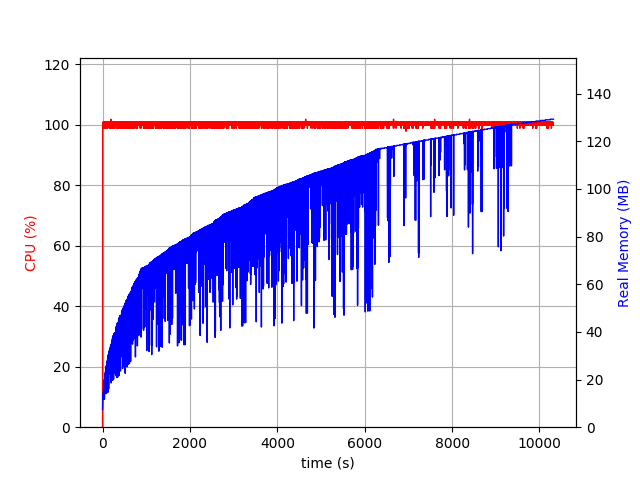
(a) Box

(b) SymBox

(c) TZono

(d) SymTZono

(e) EZono

(f) SymEZono

Figure 4: CPU and memory usage

According to memory footprint, both AI²-r and Symb with T-Zonotope or E-Zonotope need more memory than them with Box do, and will crash on large networks, such as CNN2, because of running out of memory. Figure 4 shows how CPU and resident memory usage change over time. The horizontal axis in the figure is the time, in seconds, the vertical axis corresponding to the red line is the CPU usage percentage, and the vertical axis corresponding to the blue line is the memory usage, in MB.

Greater Verifiable Robustness Bounds

Table 1(b) shows the results of using the obtained bounds to help verify the robustness property. We consider a few thresholds for robustness tolerance, i.e., $\{0.1,0.2,0.3,0.4,0.5,0.6\}$, and find that Symb can verify many more cases than AI²-r do with comparable time consumption (less than 2x in most cases, and sometimes even faster).

Proportion of Activated/Deactivated ReLU Nodes

Table 1(c) reports the number of hidden neurons whose ReLU behaviour (i.e., activated or deactivated) has been consistent within the tolerance $\delta$. Compared to AI²-r, our Symb can decide the ReLU behaviour with a much higher percentage.

$\delta$	AI2-r		Symb			Planet
	TZono	EZono	Box	TZono	EZono
0.1	7.13046%	7.08137%	6.15622%	6.15622%	6.15622%	5.84974%
0.2	11.09230%	10.88775%	6.92011%	6.92011%	6.92011%	6.11095%
0.3	18.75853%	18.32059%	8.21241%	8.21241%	8.21241%	6.50692%
0.4	30.11872%	29.27580%	10.31225%	10.31225%	10.31225%	7.04413%
0.5	45.13963%	44.25026%	14.49276%	14.49276%	14.49276%	7.96402%
0.6	55.67772%	54.88288%	20.03251%	20.03251%	20.03251%	9.02688%

Table 2: Bound proportions (smaller is better) for 1000 randomly sampled pictures from MNIST testing set on FNN1 with $\delta\in\{0.1,0.2,0.3,0.4,0.5,0.6\}$.

We remark that, although the experimental results presented above are based on $3$ fixed inputs, more extensive experiments have already been conducted to confirm that the conclusions are general. We randomly sample 1000 pictures (100 pictures per label) from the MNIST dataset, and compute the bound proportion for each of the pair $(m,\delta)$ where $m$ refers to the seven approaches in Table 1 and $\delta\in\{0.1,0.2,0.3,0.4,0.5,0.6\}$ on FNN1. Each entry corresponding to $(m,\delta)$ in Table (2) is the average of bound proportions of approach $m$ over 1000 pictures and fixed tolerance $\delta$. Then we get the average of the bound proportion of AI²-r with TZono/EZono, Symb with Box/TZono/EZono, and Planet over six different tolerances are $27.98623\%$,$27.44977\%$,$11.02104\%$, $11.02104\%$, $11.02104\%$, $7.08377\%$, respectively, which are very close to the first row of Table 1(a).

Comparison with the bounded powerset domain

In AI² [10], the bounded powerset domains are used to improve the precision. In AI²-r, we also implemented such bounded powerset domains instantiated by Box, T-Zonotope and E-Zonotope domains, with 32 as the bound of the number of the abstract elements in a disjunction. The comparison of the performance on the powerset domains with our symbolic propagation technique (with underlying domains rather than powerset domains) is shown in Table 3. We can see that our technique is much more precise than the powerset domains. The time and memory consumptions of the powerset domains are both around 32 times as much as the underlying domains, which are more than those of our technique.

	AI2-r			Symb			Planet
	Box32	TZono32	EZono32	Box	TZono	EZono
FNN1	89.65790%	20.68675%	15.87726%	9.69327%	9.69327%	9.69327%	7.05553%
FNN2	89.42070%	16.27651%	8.18317%	1.76704%	1.76704%	1.76704%	0.89089%
FNN3	89.43396%	21.98109%	12.42840%	6.88656%	6.88656%	6.88656%	4.51223%
FNN4	89.44806%	25.97855%	13.05969%	5.13645%	5.13645%	5.13645%	2.71537%
FNN5	89.16034%	29.61022%	17.88676%	3.34578%	3.34578%	3.34578%	0.14836%
FNN6	89.30790%	OOM	22.60030%	7.12480%	7.12480%	7.12480%	1.94230%
FNN7	88.62267%	OOM	1h TIMEOUT	5.52267%	5.52267%	5.52267%	1h TIMEOUT

Table 3: Bound proportions (smaller is better) of different abstract interpretation approaches with the robustness bound $\delta\in\{0.1,0.2,0.3,0.4,0.5,0.6\}$, and the fixed input pictures 767, 1955, and 2090. Note that each entry gives the average bound proportion over six different tolerance and three pictures.

Faster Verification

				$\delta=0.1$			$\delta=0.075$			$\delta=0.05$			$\delta=0.025$			$\delta=0.01$				Total
				Result	Time		Result	Time		Result	Time		Result	Time		Result	Time			Time
Point 1	Reluplex			SAT	39		SAT	123		SAT	14		UNSAT	638		UNSAT	64			879
	Reluplex + ABS			SAT	45		SAT	36		SAT	14		UNSAT	237		UNSAT	36			368
Point 2	Reluplex			UNSAT	6513		UNSAT	1559		UNSAT	319		UNSAT	49		UNSAT	11			8451
	Reluplex + ABS			UNSAT	141		UNSAT	156		UNSAT	75		UNSAT	40		UNSAT	0			412
Point 3	Reluplex			UNSAT	1013		UNSAT	422		UNSAT	95		UNSAT	79		UNSAT	6			1615
	Reluplex + ABS			UNSAT	44		UNSAT	71		UNSAT	0		UNSAT	0		UNSAT	0			115
Point 4	Reluplex			SAT	3		SAT	5		SAT	1236		UNSAT	579		UNSAT	8			1831
	Reluplex + ABS			SAT	3		SAT	7		UNSAT	442		UNSAT	31		UNSAT	0			483
Point 5	Reluplex			UNSAT	14301		UNSAT	4248		UNSAT	1392		UNSAT	269		UNSAT	6			20216
	Reluplex + ABS			UNSAT	2002		UNSAT	1402		UNSAT	231		UNSAT	63		UNSAT	0			3698

Table 4: The satisfiability on given $\delta$, and the time (in second) with and without bounds generated by abstract interpretation with symbolic propagation on the Box domain.

In this part we use the networks of ACAS Xu. To evaluate the benefits of tighter bounds for SMT-based tools, we give the bounds obtained by abstract interpretation (on Box domain with symbolic propagation) to Reluplex [15] and observe the performance difference. The results are shown in Table 4. Each cell shows the satisfiability (i.e., SAT if an adversarial example is found) and the running time without or with given bounds. The experiments are conducted on different $\delta$ values (as in [15]) and a fixed network (nnet1_1 [15]) and 5 fixed points (Point 1 to 5 in [15]). The running time our technique spends on deriving the bounds are all less than $1$ second. Table 4 shows that tighter initial bounds bring significant benefits to Reluplex with an overall $({\frac{1}{5076}-\frac{1}{32992})}/{\frac{1}{32992}}=549.43\%$ speedup (9.16 hours compared to 1.41 hours). However, it should be noted that, on one specific case (i.e., $\delta=0.1$ at Point 1 and $\delta=0.075$ at point 4), the tighter initial bounds slow Reluplex, which means that the speedup is not guaranteed on all cases. For the case $\delta=0.05$ at point 4, Reluplex gives SAT and Reluplex+ABS gives UNSAT. This may result from a floating point arithmetic error.

7 Related Work

Verification of neural networks can be traced back to [24], where the network is encoded after approximating every sigmoid activation function with a set of piecewise linear constraints and then solved with an SMT solver. It works with a network of 6 hidden nodes. More recently, by considering DNNs with ReLU activation functions, the verification approaches include constraint-solving [15, 18, 8, 20], layer-by-layer exhaustive search [12], global optimisation [25, 5, 26], abstract interpretation [10, 28, 29], functional approximation [36], and reduction to two-player game [33, 35], etc. More specifically, [15] presents an SMT solver Reluplex to verify properties on DNNs with fully-connected layers. [8] presents another SMT solver Planet which combines linear approximation and interval arithmetic to work with fully connected and max pooling layers. Methods based on SMT solvers do not scale well, e.g., Reluplex can only work with DNNs with a few hidden neurons.

The above works are mainly for the verification of local robustness. Research has been conducted to compute other properties, e.g., the output reachability. An exact computation of output reachability can be utilised to verify local robustness. In [4], Sherlock, an algorithm based on local and global search and mixed integer linear programming (MILP), is put forward to calculate the output range of a given label when the inputs are restricted to a small subspace. [25] presents another algorithm for output range analysis, and their algorithm is workable for all Lipschitz continuous DNNs, including all layers and activation functions mentioned above. In [31], the authors use symbolic interval propagation to calculate output range. Compared with [31], our approach fits for general abstract domains, while their symbolic interval propagation is designed specifically for symbolic intervals.

AI²[10] is the first to use abstract interpretation to verify DNNs. They define a class of functions called conditional affine transformations (CAT) to characterize DNNs containing fully connected, convolutional and max pooling layers with the ReLU activation function. They use Interval and Zonotope as the abstract domains and the powerset technique on Zonotope. Compared with AI², we use symbolic propagation rather than powerset extension techniques to enhance the precision of abstract interpretation based DNN verification. Symbolic propagation is more lightweight than powerset extension. Moreover, we also use the bounds information given by abstract interpretation to accelerate SMT based DNN verification. DeepZ [28] and DeepPoly [29] propose two specific abstract domains tailored to DNN verification, in order to improve the precision of abstract interpretation on the verification on DNNs. In contrast, our work is a general approach that can be applied on various domains.

8 Conclusion

In this paper, we have explored more potential of abstract interpretation on the verification over DNNs. We have proposed to use symbolic propagation on abstract interpretation to take advantage of the linearity in most part of the DNNs, which achieved significant improvements in terms of the precision and memory usage. This is based on a key observation that, for local robustness verification of DNNs where a small region of the input space is concerned, a considerable percentage of hidden neurons remain active or inactive for all possible inputs in the region. For these neurons, their ReLU activation function can be replaced by a linear function. Our symbolic propagation iteratively computes for each neuron this information and utilize the computed information to improve the performance.

This paper has presented with formal proofs three somewhat surprising theoretical results, which are then affirmed by our experiments. These results have enhanced our theoretical and practical understanding about the abstract interpretation based DNN verification and symbolic propagation.

This paper has also applied the tighter bounds of variables on hidden neurons from our approach to improve the performance of the state-of-the-art SMT based DNN verification tools, like Reluplex. The speed-up rate is up to 549% in our experiments. We believe this result sheds some light on the potential in improving the scalability of SMT-based DNN verification: In addition to improving the performance through enhancing the SMT solver for DNNs, an arguably easier way is to take an abstract interpretation technique (or other techniques that can refine the constraints) as a pre-processing.

References

- [1] Deep neural networks for acoustic modeling in speech recognition: The shared views of four research groups. IEEE Signal Process. Mag. 29(6), 82–97 (2012). https://doi.org/10.1109/MSP.2012.2205597, https://doi.org/10.1109/MSP.2012.2205597
- [2] Carlini, N., Wagner, D.: Towards evaluating the robustness of neural networks. In: Security and Privacy (SP), 2017 IEEE Symposium on. pp. 39–57. IEEE (2017)
- [3] Cousot, P., Cousot, R.: Abstract interpretation: A unified lattice model for static analysis of programs by construction or approximation of fixpoints. In: Fourth ACM Symposium on Principles of Programming Languages (POPL). pp. 238–252 (1977)
- [4] Dutta, S., Jha, S., Sankaranarayanan, S., Tiwari, A.: Output range analysis for deep feedforward neural networks. In: Dutle, A., Muñoz, C.A., Narkawicz, A. (eds.) NASA Formal Methods - 10th International Symposium, NFM 2018, Newport News, VA, USA, April 17-19, 2018, Proceedings. Lecture Notes in Computer Science, vol. 10811, pp. 121–138. Springer (2018). https://doi.org/10.1007/978-3-319-77935-5_9, https://doi.org/10.1007/978-3-319-77935-5_9
- [5] Dutta, S., Jha, S., Sankaranarayanan, S., Tiwari, A.: Output range analysis for deep feedforward neural networks. In: Dutle, A., Muñoz, C., Narkawicz, A. (eds.) NASA Formal Methods. pp. 121–138. Springer International Publishing, Cham (2018)
- [6] Dvijotham, K., Stanforth, R., Gowal, S., Mann, T.A., Kohli, P.: A dual approach to scalable verification of deep networks. CoRR abs/1803.06567 (2018), http://arxiv.org/abs/1803.06567
- [7] Dy, J.G., Krause, A. (eds.): Proceedings of the 35th International Conference on Machine Learning, ICML 2018, Stockholmsmässan, Stockholm, Sweden, July 10-15, 2018, JMLR Workshop and Conference Proceedings, vol. 80. JMLR.org (2018), http://proceedings.mlr.press/v80/
- [8] Ehlers, R.: Formal verification of piece-wise linear feed-forward neural networks. In: 15th International Symposium on Automated Technology for Verification and Analysis (ATVA2017). pp. 269–286 (2017)
- [9] von Essen, C., Giannakopoulou, D.: Analyzing the next generation airborne collision avoidance system. In: Ábrahám, E., Havelund, K. (eds.) Tools and Algorithms for the Construction and Analysis of Systems - 20th International Conference, TACAS 2014, Held as Part of the European Joint Conferences on Theory and Practice of Software, ETAPS 2014, Grenoble, France, April 5-13, 2014. Proceedings. Lecture Notes in Computer Science, vol. 8413, pp. 620–635. Springer (2014). https://doi.org/10.1007/978-3-642-54862-8_54, https://doi.org/10.1007/978-3-642-54862-8_54
- [10] Gehr, T., Mirman, M., Drachsler-Cohen, D., Tsankov, P., Chaudhuri, S., Vechev, M.: AI2: Safety and robustness certification of neural networks with abstract interpretation. In: 2018 IEEE Symposium on Security and Privacy (S&P 2018). pp. 948–963 (2018)
- [11] Ghorbal, K., Goubault, E., Putot, S.: The zonotope abstract domain taylor1+. In: International Conference on Computer Aided Verification. pp. 627–633. Springer (2009)
- [12] Huang, X., Kwiatkowska, M., Wang, S., Wu, M.: Safety verification of deep neural networks. In: 29th International Conference on Computer Aided Verification (CAV2017). pp. 3–29 (2017)
- [13] Jeannin, J., Ghorbal, K., Kouskoulas, Y., Gardner, R., Schmidt, A., Zawadzki, E., Platzer, A.: Formal verification of ACAS x, an industrial airborne collision avoidance system. In: Girault, A., Guan, N. (eds.) 2015 International Conference on Embedded Software, EMSOFT 2015, Amsterdam, Netherlands, October 4-9, 2015. pp. 127–136. IEEE (2015). https://doi.org/10.1109/EMSOFT.2015.7318268, https://doi.org/10.1109/EMSOFT.2015.7318268
- [14] Julian, K.D., Kochenderfer, M.J., Owen, M.P.: Deep neural network compression for aircraft collision avoidance systems. CoRR abs/1810.04240 (2018), http://arxiv.org/abs/1810.04240
- [15] Katz, G., Barrett, C.W., Dill, D.L., Julian, K., Kochenderfer, M.J.: Reluplex: An efficient SMT solver for verifying deep neural networks. In: 29th International Conference on Computer Aided Verification (CAV2017). pp. 97–117 (2017)
- [16] Krizhevsky, A., Sutskever, I., Hinton, G.E.: Imagenet classification with deep convolutional neural networks. In: Bartlett, P.L., Pereira, F.C.N., Burges, C.J.C., Bottou, L., Weinberger, K.Q. (eds.) Advances in Neural Information Processing Systems 25: 26th Annual Conference on Neural Information Processing Systems 2012. Proceedings of a meeting held December 3-6, 2012, Lake Tahoe, Nevada, United States. pp. 1106–1114 (2012), http://papers.nips.cc/paper/4824-imagenet-classification-with-deep-convolutional-neural-networks
- [17] Lécun, Y., Bottou, L., Bengio, Y., Haffner, P.: Gradient-based learning applied to document recognition. Proceedings of the IEEE 86(11), 2278–2324 (1998)
- [18] Lomuscio, A., Maganti, L.: An approach to reachability analysis for feed-forward ReLU neural networks. In: KR2018 (2018)
- [19] Miné, A.: Tutorial on static inference of numeric invariants by abstract interpretation. Foundations and Trends in Programming Languages 4(3-4), 120–372 (2017)
- [20] Narodytska, N., Kasiviswanathan, S.P., Ryzhyk, L., Sagiv, M., Walsh, T.: Verifying properties of binarized deep neural networks. arXiv preprint arXiv:1709.06662 (2017)
- [21] Neumaier, A., Shcherbina, O.: Safe bounds in linear and mixed-integer linear programming. Math. Program. 99(2), 283–296 (2004). https://doi.org/http://dx.doi.org/10.1007/s10107-003-0433-3
- [22] Nguyen, A., Yosinski, J., Clune, J.: Deep neural networks are easily fooled: High confidence predictions for unrecognizable images. In: Proceedings of the IEEE Conference on Computer Vision and Pattern Recognition. pp. 427–436 (2015)
- [23] Papernot, N., McDaniel, P.D., Jha, S., Fredrikson, M., Celik, Z.B., Swami, A.: The limitations of deep learning in adversarial settings. CoRR abs/1511.07528 (2015), http://arxiv.org/abs/1511.07528
- [24] Pulina, L., Tacchella, A.: An abstraction-refinement approach to verification of artificial neural networks. In: Touili, T., Cook, B., Jackson, P.B. (eds.) Computer Aided Verification, 22nd International Conference, CAV 2010, Edinburgh, UK, July 15-19, 2010. Proceedings. Lecture Notes in Computer Science, vol. 6174, pp. 243–257. Springer (2010). https://doi.org/10.1007/978-3-642-14295-6_24, https://doi.org/10.1007/978-3-642-14295-6_24
- [25] Ruan, W., Huang, X., Kwiatkowska, M.: Reachability analysis of deep neural networks with provable guarantees. In: Lang, J. (ed.) Proceedings of the Twenty-Seventh International Joint Conference on Artificial Intelligence, IJCAI 2018, July 13-19, 2018, Stockholm, Sweden. pp. 2651–2659. ijcai.org (2018). https://doi.org/10.24963/ijcai.2018/368, https://doi.org/10.24963/ijcai.2018/368
- [26] Ruan, W., Wu, M., Sun, Y., Huang, X., Kroening, D., Kwiatkowska, M.: Global robustness evaluation of deep neural networks with provable guarantees for the hamming distance. In: IJCAI2019 (2019)
- [27] Silver, D., Huang, A., Maddison, C.J., Guez, A., Sifre, L., van den Driessche, G., Schrittwieser, J., Antonoglou, I., Panneershelvam, V., Lanctot, M., Dieleman, S., Grewe, D., Nham, J., Kalchbrenner, N., Sutskever, I., Lillicrap, T.P., Leach, M., Kavukcuoglu, K., Graepel, T., Hassabis, D.: Mastering the game of go with deep neural networks and tree search. Nature 529(7587), 484–489 (2016). https://doi.org/10.1038/nature16961, https://doi.org/10.1038/nature16961
- [28] Singh, G., Gehr, T., Mirman, M., Püschel, M., Vechev, M.T.: Fast and effective robustness certification. In: Bengio, S., Wallach, H.M., Larochelle, H., Grauman, K., Cesa-Bianchi, N., Garnett, R. (eds.) Advances in Neural Information Processing Systems 31: Annual Conference on Neural Information Processing Systems 2018, NeurIPS 2018, 3-8 December 2018, Montréal, Canada. pp. 10825–10836 (2018), http://papers.nips.cc/paper/8278-fast-and-effective-robustness-certification
- [29] Singh, G., Gehr, T., Püschel, M., Vechev, M.T.: An abstract domain for certifying neural networks. PACMPL 3(POPL), 41:1–41:30 (2019), https://dl.acm.org/citation.cfm?id=3290354
- [30] Szegedy, C., Zaremba, W., Sutskever, I., Bruna, J., Erhan, D., Goodfellow, I., Fergus, R.: Intriguing properties of neural networks. In: International Conference on Learning Representations (ICLR2014) (2014)
- [31] Wang, S., Pei, K., Whitehouse, J., Yang, J., Jana, S.: Formal security analysis of neural networks using symbolic intervals. CoRR abs/1804.10829 (2018), http://arxiv.org/abs/1804.10829
- [32] Weng, T., Zhang, H., Chen, H., Song, Z., Hsieh, C., Daniel, L., Boning, D.S., Dhillon, I.S.: Towards fast computation of certified robustness for relu networks. In: Dy and Krause [7], pp. 5273–5282, http://proceedings.mlr.press/v80/weng18a.html
- [33] Wicker, M., Huang, X., Kwiatkowska, M.: Feature-guided black-box safety testing of deep neural networks. In: International Conference on Tools and Algorithms for the Construction and Analysis of Systems (TACAS2018). pp. 408–426. Springer (2018)
- [34] Wong, E., Kolter, J.Z.: Provable defenses against adversarial examples via the convex outer adversarial polytope. In: Dy and Krause [7], pp. 5283–5292, http://proceedings.mlr.press/v80/wong18a.html
- [35] Wu, M., matthew Wicker, Ruan, W., Huang, X., Kwiatkowska, M.: A game-based approximate verification of deep neural networks with provable guarantees. Theoretical Computer Science (5 2019)
- [36] Xiang, W., Tran, H., Johnson, T.T.: Output reachable set estimation and verification for multilayer neural networks. IEEE Transactions on Neural Networks and Learning Systems 29(11), 5777–5783 (Nov 2018). https://doi.org/10.1109/TNNLS.2018.2808470