Numerical stochastic perturbation theory applied to the twisted Eguchi-Kawai model

Abstract

We present the results of an exploratory study of the numerical stochastic perturbation theory (NSPT) applied to the four dimensional twisted Eguchi-Kawai (TEK) model. We employ a Kramers type algorithm based on the Generalized Hybrid Molecular Dynamics (GHMD) algorithm. We have computed the perturbative expansion of square Wilson loops up to $O(g^{8})$. The results of the first two coefficients (up to $O(g^{4})$) have a high precision and match well with the exact values. The next two coefficients can be determined and even extrapolated to large $N$, where they should coincide with the corresponding coefficients for ordinary Yang-Mills theory on an infinite lattice. Our analysis shows the behaviour of the probability distribution for each coefficient tending to Gaussian for larger $N$. The results allow us to establish the requirements to extend this analysis to much higher order.

1 Introduction

Gauge theories in the limit of infinite number of colours ($N\longrightarrow\infty$) are very interesting theoretically tHooft:1973alw . They are simpler than their finite $N$ counterparts, but share most of the fascinating properties of the latter. Nonetheless, their understanding remains a challenge. The relevance of this goal is also given by the fact that they seem a point of contact with other approaches Maldacena:1997re . A good deal of their difficulty lies in the non-perturbative character of most of its properties. The standard first principles approach to this kind of problems is the lattice formulation of quantum field theory Wilson:1974sk . However, in contrast with what happens in perturbation theory, the large $N$ limit involves an extrapolation and seems harder than the finite $N$ study. Only recently this line of approach has led to trustworthy computations (for a review see  Lucini:2012gg ), pioneered by the works of Teper and collaborators Lucini:2003zr ; Lucini:2004my ; Lucini:2005vg .

Fortunately, there is a very specific simplification which emerges when studying large $N$ gauge theories on the lattice. This is the so-called Eguchi-Kawai (EK) reduction Eguchi:1982nm . According to this result finite volume corrections are subleading in the large $N$ limit. Hence, there is the possibility that the dynamics of the large $N$ gauge theories is captured by a matrix model. There are several proposals that have been put forward to transform this possibility into a reality Bhanot:1982sh ; Gross:1982at ; Narayanan:2003fc ; Kovtun:2007py ; Unsal:2008ch . Here, we will be concerned with one of the early proposals called Twisted Eguchi-Kawai model (TEK for short) GonzalezArroyo:1982ub ; GonzalezArroyo:1982hz , and introduced by two of the present authors. Indeed, it was used shortly after EK proposal to compute the string tension at large $N$ GonzalezArroyo:1983pw ; Fabricius:1984un . Lately this has led to a calculation of this quantity with at least compatible precision to other methods GonzalezArroyo:2012fx . Several precise tests of the reduction mechanism have been obtained recently for other quantities Gonzalez-Arroyo:2014dua , providing a strong verification of the validity and usefulness of this approach.

The previous paragraph justifies our interest in the TEK model. The finite $N$ corrections are different for the matrix model and for the ordinary gauge theory, and their size and nature are very important from the practical point of view, in order to make this approach competitive computationally. Curiously, these corrections have a theoretically interesting interpretation in terms of the so-called non-commutative gauge theories Douglas:2001ba . Their Lagrangian and Feynman rules first appeared in the literature GonzalezArroyo:1983ac when looking for a continuous generalization of the TEK model, and before they emerged from the mathematical construction of non-commutative geometries Connes:1987ue . A more direct connection appears as a result of Morita duality on the non-commutative torus. This shows that ordinary gauge theories with twisted boundary conditions (TBC) a la ’t Hooft tHooft:1979rtg are particular cases of non-commutative field theories. The TEK model is nothing but the volume reduced version of a gauge theory with twisted boundary conditions on the lattice. TBC are characterized by a collection of integer-valued fluxes, and their appropriate choice has been found to have a crucial impact upon the size of the corrections and the absence of phase transitions.

The last ingredient entering in this work is perturbation theory. Although our major interest when using the lattice approach was in studying the non-perturbative aspects of the theory, there is also interest in understanding the theory from the perturbative side. At the least it offers us a method to analytically determine certain observables and estimating the size and nature of its $N$ dependence. In this spirit a recent perturbative calculation of Wilson loops in lattice gauge theories with twisted boundary conditions (including the TEK model) was addressed Perez:2017jyq .

In addition, a new set of ideas has focused in explaining the usefulness of perturbation theory in understanding also non-perturbative contributions. This takes its most extreme form in the concept of resurgence (see for example Dunne:2015eaa ; Cherman:2014ofa and references therein). At the least, as was already known, the large order behaviour of the perturbative coefficients is associated with non-perturbative aspects such as the action of other saddles. Very interesting results have been obtained in this spirit for large $N$ matrix theories Cherman:2014ofa ; Marino:2012zq . For example, it has been identified that the large $N$ phase transition of the Gross-Witten-Wadia unitary matrix model Gross:1980he ; Wadia:2012fr is governed by non-trivial saddles and the action can be reconstructed via the resurgence on the asymptotic expansion about the vacuum Buividovich:2015oju .

For large $N$ gauge theories in 4 dimensions there are many interesting aspects to be studied. Perturbation theory is dominated by planar diagrams, whose number does not grow factorially. This could suggest that the perturbative series is convergent within a given radius. Furthermore, the instanton action at fixed value of ’t Hooft coupling diverges. This implies that the corresponding singularity in the Borel plane moves to infinity, suggesting at least Borel summability. However, the expected singularity associated to infrared renormalons tHooft:1977xjm ; Beneke:1998ui does not move away and would induce a factorial growth of the coefficients similar to the finite $N$ case. An analysis of the perturbative expansion at high orders should settle this point. Another issue to be studied is the interplay between the order of perturbation theory and the value of $N$. The higher rate of growth in the number of non-planar diagrams would suggest that their contribution could overcome the $1/N^{2}$ suppression at sufficiently high orders. Something of this kind emerges when analyzing the simultaneous expansion in powers of ’t Hooft coupling and $1/N^{2}$ as seen in Ref. Marino:2012zq . The behaviour of the reduced model could however be quite different.

To close the circle, recently a new method has arisen that allows the numerical computation of high order coefficients in the perturbative expansion. It goes under the name of Numerical Stochastic perturbation theory (NSPT) and was pioneered by the works of Di Renzo and collaborators DiRenzo:1993hs ; DiRenzo:1994av ; DiRenzo:1994sy ; DiRenzo:1995qc ; Burgio:1997hc ; DiRenzo:2004hhl (for earlier developments on stochastic quantization Parisi:1980ys and stochastic perturbation theory, see also Damgaard:1987rr ; BOOK_SQ1 ; BOOK_SQ2 ). Recently, this methodology has led to remarkable results about high order coefficients in SU(3) gauge theories DiRenzo:2000ua ; Rakow:2005yn ; Bauer:2011ws ; Horsley:2012ra ; Bali:2013pla ; Horsley:2013pra ; Bali:2014fea ; DelDebbio:2018ftu ; DelDebbio:2018vhr . As the memory size required is proportional to the highest perturbation order involved in the computation in NSPT and to the volume, the authors of Bali:2013pla ; Bali:2014fea ; DelDebbio:2018ftu have used twisted boundary conditions aware that they lead to reduced finite volume dependence.

Stochastic quantization is based on the Langevin equation, and the first NSPT studies used the perturbative expansion of this equation. However, for lattice theories various other Monte Carlo algorithms, such as Kramers, hybrid molecular dynamics (HMD), and hybrid Monte Carlo (HMC) algorithms, have been developed and used. Recently, extensive studies have been carried out using NSPT algorithms DallaBrida:2017pex ; DallaBrida:2017tru based on them. In particular, the HMD based algorithm for NSPT is easy to implement by perturbatively expanding the HMD/HMC codes used for non-perturbative simulations. In this case, one can benefit from various numerical integration schemes for the molecular dynamics part to reduce the finite step size error of the integration. Thus, the NSPT algorithm based on the HMD/HMC algorithm could open the way to efficiently estimating very high order coefficients.

Our work is a first attempt to apply this methodology to matrix models. For the time being, our work is mostly exploratory but a necessary step before any attempt of a higher order and larger $N$ study. Nonetheless, apart from showing that the method works with an incredibly high precision for the low-order coefficients, we also present results which extend to higher order the previous analytical results Perez:2017jyq . In addition, our work provides interesting information about the probability distribution of the perturbative coefficients. In particular, we have studied the dependence of the cumulants of these distributions with respect to the different parameters: the value of $N$ and of the fluxes, the size of the loops and the order of perturbation theory. These results allow us to determine the necessary computational requirements for any further extension of these studies.

The layout of the paper is the following. In section 2, after introducing the TEK model, we explain the application of the NSPT algorithm based on the HMD algorithm to the TEK model. In Section 3 we present the numerical results for the perturbative coefficients of the Wilson loops. We employ $(N,k)=(16,1),(49,2),(121,3)$ for $\mathrm{SU}(N)$ and flux parameter $k$ of the TEK model. The coefficients are computed up to four-loop ($O(g^{8})$) and the first two-loop coefficients are compared to the analytic values. The probability distribution of these estimates is investigated and used to explore the feasibility for extending our results to higher orders. We estimate the numerical computational cost of NSPT for the TEK model at large values of $N$ and large perturbative orders in section 4. Possible improvements on the algorithm are also discussed. In the last section we summarize the main results of the paper. Two technical points are included in appendices.

2 TEK model and NSPT

In this section we start by briefly introducing the TEK model together with the gauge fixing method. Then we recall the Hybrid Molecular Dynamics (HMD) algorithm for nonperturbative simulations of the TEK model. This algorithm is then perturbatively expanded to derive the equation of motion for the NSPT algorithm.

The computational cost is estimated in terms of the highest order $N_{\mathrm{trunc}}$ in the perturbative expansion involved in the algorithm and the matrix size $N$ of $\mathrm{SU}(N)$.

2.1 TEK model

The partition function of the TEK model in four-dimensions is defined by

$$Z =\int\prod_{\mu=1}^{4}\mathrm{d}U_{\mu}\,e^{-S[U]},$$ (1)

$$S[U] =\beta\sum_{\mu,\nu=1,\mu\neq\nu}^{4}\operatorname{Tr}\left[I-z_{\mu\nu}U_{\mu}U_{\nu}U_{\mu}^{{\dagger}}U_{\nu}^{{\dagger}}\right],$$ (2)

where $U_{\mu}$ are $\mathrm{SU}(N)$ matrices. We choose the symmetric twist characterized by $N=\hat{L}^{2}$ and $z_{\mu\nu}$ given by

$$z_{\mu\nu} =\exp\left[\dfrac{2\pi i}{N}n_{\mu\nu}\right],$$

$$n_{\mu\nu} =\epsilon_{\mu\nu}k\hat{L},$$

$$\epsilon_{\mu\nu} =\left\{\begin{matrix}+1&\quad\mbox{for $\mu<\nu$}\\ 0&\quad\mbox{for $\mu=\nu$}\\ -1&\quad\mbox{for $\mu>\nu$}\end{matrix}\right.,$$ (3)

where $k$ is an integer coprime with $\hat{L}$ ($=\sqrt{N}$). The bare coupling constant $g$ is defined through $\beta=1/g^{2}$.

The Wilson loop operator for an $R\times T$ rectangle in the $\mu$–$\nu$ plane is defined by

$$W_{\mu\nu}(R,T) =\dfrac{1}{N}\left(z_{\mu\nu}\right)^{RT}\operatorname{Tr}\left[\left(U_{\mu}\right)^{R}\left(U_{\nu}\right)^{T}\left(U_{\mu}^{{\dagger}}\right)^{R}\left(U_{\nu}^{{\dagger}}\right)^{T}\right].$$ (4)

In this paper we restrict ourselves to square loops $R=T$.

The analytic perturbative expansion of the observables proceeds by expanding the link matrices around the classical vacuum as

$$U_{\mu}=e^{-igA_{\mu}}\Gamma_{\mu},$$ (5)

where the matrices $\Gamma_{\mu}$ define the classical vacuum of eq. (2) and have the following property

$$\Gamma_{\mu}\Gamma_{\nu}=\Gamma_{\nu}\Gamma_{\mu}z_{\mu\nu}^{*}.$$ (6)

A particular solution (up to multiplication by a phase) is singled out by an appropriately chosen gauge fixing condition, accompanied by the corresponding ghost term.

In order to stabilize the runaway trajectories, NSPT also requires the use of the stochastic gauge fixing method Zwanziger:1981kg . Here we are using the functional for the Landau gauge condition, from which we can extract the stochastic gauge fixing contribution in NSPT DiRenzo:1993hs ; DiRenzo:1994av . The gauge fixing functional $F[G]$ is defined by

$$F[G] =\sum_{\mu=1}^{4}\mathrm{Re}\left[\operatorname{Tr}\left[GU_{\mu}G^{{\dagger}}\Gamma_{\mu}^{{\dagger}}\right]\right],$$ (7)

where $G\in\mathrm{SU}(N)$ is the gauge transformation matrix. The Landau gauge condition is achieved by maximizing the functional, by application of several iterations of the form:

$$U_{\mu}\to U_{\mu}^{\prime}=GU_{\mu}G^{{\dagger}},$$ (8)

with

$$G =\exp\left[i\alpha\Theta\right],$$ (9)

$$\Theta =i\left[\left(Y-Y^{\dagger}\right)-\dfrac{1}{N}\operatorname{Tr}\left(Y-Y^{\dagger}\right)\right],$$ (10)

$$Y =\sum_{\mu=1}^{4}\left[U_{\mu}\Gamma_{\mu}^{{\dagger}}-\Gamma_{\mu}^{{\dagger}}U_{\mu}\right],$$ (11)

where $\alpha$ is a parameter. When this iteration process is transformed into a continuous evolution equation with a fictitious time $t$, we obtain the following differential equation:

$$G(t) =\exp\left[iw(t)\right],$$ (12)

$$\dfrac{dw}{dt} \equiv\alpha\Theta[U(t)],$$ (13)

$$U_{\mu}(t) =G(t)U_{\mu}G(t)^{{\dagger}},$$ (14)

where $w(t)$ is an auxiliary Hermitian-traceless matrix tracing the steepest descent trajectory. This evolution equation can be combined with the NSPT process to implement the stochastic gauge fixing.

2.2 NSPT for the TEK model

NSPT is based on stochastic quantization Parisi:1980ys . This amounts to writing down a stochastic differential equation of the Langevin type for the field variables of a target system, which relaxes to the equilibrium probability density at large times Damgaard:1987rr ; BOOK_SQ1 ; BOOK_SQ2 . The NSPT method is obtained by expanding these field variables in powers of the coupling constant and casting the original Langevin equation into a tower of equations, one for each power. Observables that are analytic functions of the field variables acquire a corresponding perturbative expansion. Each term in the expansion becomes an stochastic variable whose mean value at large times gives us the corresponding coefficient that we are after.

In this paper we employ the HMD based NSPT, which has been introduced in refs. DallaBrida:2017tru ; DallaBrida:2017pex . This is easy to implement through modifications of existing codes of nonperturbative HMD or HMC algorithms, and is preferable to systematically improve the molecular dynamics (MD) part, reducing the error arising from the finite MD step size.

To explain the method in our case, we will begin by reviewing the generalized HMD (GHMD) algorithm for nonperturbative simulations. Then we will apply the perturbative expansion to the algorithm, to derive the HMD based NSPT algorithm.

The HMD partition function is introduced by adding the canonical momentum variable $P_{\mu}$ conjugate to $U_{\mu}$ to the original partition function eq. (1).

$$Z_{\mathrm{HMD}} =\int\prod_{\mu=1}^{4}\mathrm{d}U_{\mu}\prod_{\mu=1}^{4}\mathrm{d}P_{\mu}\,e^{-H[P,U]},$$ (15)

$$H[P,U] =\dfrac{1}{2}\sum_{\mu=1}^{4}\operatorname{Tr}\left[P_{\mu}P_{\mu}\right]+S[U].$$ (16)

The classical dynamics for $(P_{\mu},U_{\mu})$ with the Hamiltonian $H[P,U]$ reproduces the microcanonical ensemble at fixed energy $E=H[P,U]$. Subsequent refreshment of the variable $P_{\mu}$ with the Gaussian distributions generates the corresponding canonical ensemble $e^{-H[P,U]}$. The marginal distribution for $U_{\mu}$ becomes the $e^{-S[U]}$ distribution that we are looking for.

Algorithm 1 HMD algorithm for nonperturbative simulations

  Step 0: Set initial state $U_{0,\mu}$ arbitrary.

  Step 1: Set initial momentum $P_{0,\mu}$ from the Gaussian distribution as

$$P_{0,\mu} =\sum_{a=1}^{N^{2}-1}\eta_{\mu}^{a}T^{a}\equiv\eta_{\mu},$$ (17)

$$\mathrm{Prob}(\eta_{\mu}^{a})d\eta^{a} \propto\exp(-(\eta_{\mu}^{a})^{2}/4)d\eta^{a},$$ (18)

where the matrices $T^{a}$ are $\mathrm{SU}(N)$ generators in the fundamental representation normalized as $\mathrm{Tr}(T^{a}T^{b})=\frac{1}{2}\delta_{ab}$.

  Step 2: Solve the MD equation defined by

$$\dot{U}_{\mu} =iP_{\mu}U_{\mu},$$ (19)

$$\dot{P}_{\mu} =F_{\mu},$$ (20)

$$F_{\mu} \equiv i\beta\left[\left[S_{\mu}-S_{\mu}^{{\dagger}}\right]-\dfrac{1}{N}\operatorname{Tr}\left[S_{\mu}-S_{\mu}^{{\dagger}}\right]\right],$$ (21)

$$S_{\mu} \equiv U_{\mu}\left[\sum_{\nu=1,\nu\neq\mu}^{4}\left(z_{\mu\nu}U_{\nu}U_{\mu}^{{\dagger}}U_{\nu}^{{\dagger}}+z_{\mu\nu}^{*}U_{\nu}^{{\dagger}}U_{\mu}^{{\dagger}}U_{\nu}\right)\right],$$ (22)

from the initial state $(P_{0,\mu},U_{0,\mu})$ for a fixed interval in fictitious time. The dot $\dot{\ }$ represents the left-wise derivative with respect to the fictitious time. These evolution equations preserve the energy value $E=H[P,U]$.

  Step 3: Store $U_{\mu}$ as the configuration and set $U_{0,\mu}=U_{\mu}$, then return to Step 1.

The HMD algorithm proceeds as described in Algorithm 1, where the equations in Step 2 are discretized in time. This discretization violates the exact energy conservation, which distorts the distribution shape. In order to ensure that the discretized Markov chain leads to the correct probability distribution the Monte Carlo process must satisfy time reversibility and area preservation in the MD evolution, for which the leapfrog type scheme is normally used. For nonperturbative simulations, the Metropolis test can be inserted between Step 1 and 2 to compensate the violation of energy conservation, yielding the HMC algorithm.

The full momentum refreshment in Step 1 will cause random walking in phase space so that the autocorrelation times becomes longer for the ensemble. To relax random walking behaviour, the generalized HMC algorithm (GHMC) has been introduced in ref. Kennedy:2000ju . For the GHMC algorithm the momentum is partially refreshed in Step 1 as

$$P_{0,\mu}=c_{1}P_{\mu}+\sqrt{1-c_{1}^{2}}\,\eta_{\mu},$$ (23)

instead of eq. (17), where $c_{1}$ is a mixing parameter. $P_{\mu}$ in the right hand-side is the solution of Step 2. A momentum reflection step is added after the rejection of the Metropolis test in the GHMC algorithm, while this step is absent in the GHMD algorithm. We can further include the gauge fixing process eq. (13) into the MD evolution equation.

With the leapfrog algorithm and the partial momentum refreshment, the updating algorithm for one step having a small $\Delta t$ interval, is given by

$$\left\{\ \begin{aligned} P_{\mu}&=c_{1}P_{0,\mu}+\sqrt{1-c_{1}^{2}}\eta_{\mu},\\ w&=c_{1}w_{0},\\ U_{\mu}&=U_{0,\mu},\end{aligned}\right.$$ (24)

$$\left\{\ \begin{aligned} \bar{P}_{\mu}&=P_{\mu}+(\Delta t/2)F_{\mu}[U],\\ U_{\mu}^{\prime}&=\exp\left[i\bar{P}_{\mu}\Delta t\right]U_{\mu},\\ P_{\mu}^{\prime}&=\bar{P}_{\mu}+(\Delta t/2)F_{\mu}[U^{\prime}],\end{aligned}\right.$$ (25)

$$\left\{\ \begin{aligned} w_{1}&=w+\Delta t\alpha\Theta[U^{\prime}],\\ P_{1,\mu}&=\exp\left[iw_{1}\Delta t\right]P^{\prime}_{\mu}\exp\left[-iw_{1}\Delta t\right],\\ U_{1,\mu}&=\exp\left[iw_{1}\Delta t\right]U^{\prime}_{\mu}\exp\left[-iw_{1}\Delta t\right],\end{aligned}\right.$$ (26)

where $(P_{0,\mu},U_{0,\mu},w_{0})$ is the initial state and $(P_{1,\mu},U_{1,\mu},w_{1})$ is the final state. Eq. (25) corresponds to the leapfrog evolution for $\Delta t$, for which various higher-order schemes are available. For simplicity we will explain the second order leapfrog scheme only. The gauge fixing evolution (12)–(14) is interleaved into the MD evolution Rossi:1987hv ; Davies:1987vs and the transformation in eq. (26) does not affect the gauge invariant observables, however, we introduce this to explain the stochastic gauge fixing for NSPT Zwanziger:1981kg ; DiRenzo:1993hs ; DiRenzo:1994av . Taking the $\Delta t\to 0$ limit with $c_{1}=e^{-\gamma\Delta t}$, as shown in ref. DallaBrida:2017tru , this evolution reduces to

$$\dot{U}_{\mu} =i\left[P_{\mu}-D_{\mu}w\right]U_{\mu},$$

$$\dot{P}_{\mu} =F_{\mu}-\gamma P_{\mu}+i\left[w,P_{\mu}\right]+\zeta_{\mu},$$

$$\dot{w} =-\gamma w+\alpha\Theta,$$ (27)

where $D_{\mu}w$ is defined as

$$D_{\mu}w =U_{\mu}wU_{\mu}^{{\dagger}}-w,$$ (28)

and $\zeta_{\mu}$ is a random noise satisfying

$$\langle\zeta_{\mu}^{a}(t)\zeta_{\nu}^{b}(s)\rangle =4\gamma\delta(t-s)\delta^{a,b}\delta_{\mu,\nu}.$$ (29)

The terms with $w$ act as the gauge damping force. Eq. (27) corresponds to the Kramers equation and in the limit $\gamma\to+\infty$ ($c_{1}=0$) to the Langevin equation with gauge damping force.

In the GHMD algorithm Step 2 is obtained by repeating eqs. (25) and (26) until the total evolution time becomes a fixed value, and then applying eq. (24) to implement Step 1. When the evolution time in Step 2 reduces to $\Delta t$, the method becomes Langevin ($c_{1}=0$) or Kramers ($c_{1}\neq 0$) algorithm.

Having explained the GHMD algorithm, we now describe the corresponding NSPT algorithm. This follows by expanding $(P_{\mu},U_{\mu},w)$ and the MD equation (22) or eqs. (24)–(26) in a power series in $g$. We will now describe the perturbative expansion for eqs. (24)–(26), because it is sufficient to write the simulation program. In order to simplify notation, we first define the $\star$-product as the convolution product of two perturbative series, given by

$$C =A\star B,$$ (30)

$$A=\sum_{k=0}^{\infty}g^{k}A^{(k)},\quad B =\sum_{k=0}^{\infty}g^{k}B^{(k)},\quad C=\sum_{k=0}^{\infty}g^{k}C^{(k)},$$ (31)

$$C^{(k)}=(A\star B)^{(k)} \equiv\sum_{j=0}^{k}A^{(j)}B^{(k-j)},$$ (32)

where $A,B,C$ are matrices and $A^{(k)},B^{(k)},C^{(k)}$ are the coefficient matrices.

The perturbative expansion for $(P_{\mu},U_{\mu},w)$ is defined by

$$P_{\mu} =\beta^{1/2}\sum_{k=1}^{\infty}\beta^{-k/2}P_{\mu}^{(k)}=P_{\mu}^{(1)}+gP_{\mu}^{(2)}+g^{2}P_{\mu}^{(3)}+\dots,$$ (33)

$$U_{\mu} =\sum_{k=0}^{\infty}\beta^{-k/2}U_{\mu}^{(k)}=U_{\mu}^{(0)}+gU_{\mu}^{(1)}+g^{2}U_{\mu}^{(2)}+g^{3}U_{\mu}^{(3)}+\dots,$$ (34)

$$w =\beta^{1/2}\sum_{k=1}^{\infty}\beta^{-k/2}w^{(k)}=w^{(1)}+gw^{(2)}+g^{2}w^{(3)}+\dots,$$ (35)

where $U_{\mu}^{(0)}=\Gamma_{\mu}$ is kept fixed in NSPT as it is the perturbative vacuum. Rescaling the fictitious time and the gauge fixing parameter as $t^{\prime}=t/g$ and $\alpha^{\prime}=g^{2}\alpha$, and substituting eqs. (33)–(35) into eqs. (24)–(26), we obtain

$$\left\{\ \begin{aligned} \bar{P}_{\mu}^{(k)}&=P^{(k)}_{\mu}+(\Delta t^{\prime}/2)F^{(k)}_{\mu}[U],\\ {U^{(k)}_{\mu}}^{\prime}&=\left(\exp\left[i\bar{P}_{\mu}\Delta t^{\prime}\right]\star U_{\mu}\right)^{(k)},\\ {P^{(k)}_{\mu}}^{\prime}&=\bar{P}^{(k)}_{\mu}+(\Delta t^{\prime}/2)F^{(k)}_{\mu}[U^{\prime}],\end{aligned}\right.$$ (36)

$$\left\{\ \begin{aligned} w^{(k)}_{1}&=w^{(k)}+\Delta t^{\prime}\alpha^{\prime}\Theta^{(k)}[U^{\prime}],\\ P^{(k)}_{1,\mu}&=\left(\exp\left[iw_{1}\Delta t^{\prime}\right]\star P^{\prime}_{\mu}\star\exp\left[-iw_{1}\Delta t^{\prime}\right]\right)^{(k)},\\ U^{(k)}_{1,\mu}&=\left(\exp\left[iw_{1}\Delta t^{\prime}\right]\star U^{\prime}_{\mu}\star\exp\left[-iw_{1}\Delta t^{\prime}\right]\right)^{(k)},\end{aligned}\right.$$ (37)

for each perturbative order $k=1,2,\dots$. The details of the perturbative expansion of the matrix exponential $\exp[A]=I+g\left(\exp[A]\right)^{(1)}+g^{2}\left(\exp[A]\right)^{(2)}+\dots$ with $A=gA^{(1)}+g^{2}A^{(2)}+\dots$ are explained in Appendix A. The perturbative expressions for $F^{(k)}_{\mu}$ and $\Theta^{(k)}$ are extracted from eqs. (21)–(22), and (10)–(11), respectively:

$$F_{\mu} =\beta\sum_{k=1}^{\infty}\beta^{-k/2}F^{(k)}_{\mu},\quad\Theta=\sum_{k=1}^{\infty}\beta^{-k/2}\Theta^{(k)},$$ (38)

$$F^{(k)}_{\mu} =i\left[S^{(k)}_{\mu}-{S^{(k)}}_{\mu}^{{\dagger}}-\dfrac{1}{N}\operatorname{Tr}\left[S^{(k)}_{\mu}-{S^{(k)}}_{\mu}^{{\dagger}}\right]\right],$$ (39)

$$S^{(k)}_{\mu} =\left(U_{\mu}\star\sum_{\nu\neq\mu}\left[z_{\mu\nu}U_{\nu}\star U^{{\dagger}}_{\mu}\star U^{{\dagger}}_{\nu}+z^{*}_{\mu\nu}U^{{\dagger}}_{\nu}\star U^{{\dagger}}_{\mu}\star U_{\nu}\right]\right)^{(k)},$$ (40)

$$\Theta^{(k)} =i\left[\left(Y^{(k)}-{Y^{(k)}}^{\dagger}\right)-\dfrac{1}{N}\operatorname{Tr}\left(Y^{(k)}-{Y^{(k)}}^{\dagger}\right)\right],$$ (41)

$$Y^{(k)} =\sum_{\mu=1}^{4}\left[U^{(k)}_{\mu}\Gamma_{\mu}^{{\dagger}}-\Gamma_{\mu}^{{\dagger}}U^{(k)}_{\mu}\right].$$ (42)

In the limit $\Delta t^{\prime}\to 0$, the equation of motion should conserve the energy eq. (16) order by order in perturbation theory. This energy conservation can be monitored during the simulation.

The Wilson loop operator eq. (4) is expanded similarly:

$$W^{(k)}_{\mu\nu}(R,T) =\dfrac{\left(z_{\mu\nu}\right)^{RT}}{N}\operatorname{Tr}\left[\left(\left(U_{\mu}\right)^{\star R}\star\left(U_{\nu}\right)^{\star T}\star\left(U_{\mu}^{{\dagger}}\right)^{\star R}\star\left(U_{\nu}^{{\dagger}}\right)^{\star T}\right)^{(k)}\right],$$ (43)

where we used a shorthand notation for matrix power with the $\star$-product such as $(A\star A\star A)\equiv A^{\star 3}$. The expectation values at large times of our $W^{(k)}_{\mu\nu}(R,T)$ yield the coefficients of the perturbative expansion of Wilson loops. For the latter we take the notation given in ref. Perez:2017jyq where the first two coefficients have been computed analytically. If we consider for example an $R\times T$ Wilson loop in the $\mu$–$\nu$ plane, the relation is as follows

$$\hat{W}_{\ell}^{(R\times T)} =-N^{-\ell}\left\langle W^{(2\ell)}_{\mu\nu}(R,T)\right\rangle,$$

$$0 =\left\langle W^{(2\ell+1)}_{\mu\nu}(R,T)\right\rangle.$$ (44)

Notice that, since the perturbative expansion is in powers of ’t Hooft coupling $\lambda=g^{2}N$, the expectation value of $W^{(k)}_{\mu\nu}$ for odd values of $k$ has to vanish.

A technical point is the necessity to correct for deviations from the unitarity constraint induced by the numerical round-off error from the finite precision of computer arithmetic. While imposing the traceless-Hermitian character of $(P_{\mu}^{(k)},w^{(k)})$ is easily done, the conditions on $\{U_{\mu}^{(k)}\}$ following from the unitarity of the link matrices can be imposed by the matrix logarithm scheme for reunitarization DiRenzo:2004hhl . The details of the group projection is described in Appendix B.

Algorithm 2 NSPT algorithm based on GHMD. The MD time step size $\Delta t^{\prime}=1/N_{\mathrm{MD}}$, momentum mixing parameter $\gamma$, and gauge fixing parameter $\alpha^{\prime}$ are given.

  Step 0: Set an initial state $P^{(k)}_{0,\mu}=0,U^{(k)}_{0,\mu}=0,w^{(k)}_{0}=0$ for $k=1,\cdots$.

  Step 1: Repeat the MD evolution and gauge transformation as

  for $j=0,N_{\mathrm{MD}}-1$ do

           1-1: Compute eq. (LABEL:eq:NSPTMDinitailze) with partial momentum refreshment parameter $c_{1}=e^{-\gamma\Delta t^{\prime}}$.

           1-2: Evolve state with the discretized MD equation eq. (36) or higher order scheme for $\Delta t^{\prime}$.

           1-3: Transform state with eq. (37) for gauge fixing.

           1-4: Set $(P^{(k)}_{0,\mu},U^{(k)}_{0,\mu},w^{(k)}_{0})=(P^{(k)}_{1,\mu},U^{(k)}_{1,\mu},w^{(k)}_{1})$.

  end for

  Step 3: Project the state $(P^{(k)}_{0,\mu},U^{(k)}_{0,\mu},w^{(k)}_{0})$ out to $\mathrm{SU}(N)$ group and algebra.

  Step 4: Compute observables with ${U^{(k)}_{0,\mu}}$ and return to Step 1.

Let us conclude by summarizing our NSPT algorithm. As explained earlier, the finite time step induces a distortion in the probability distribution, which in NSPT cannot be corrected by a Metropolis test. Hence, it is preferable to employ a higher order integration scheme in the MD evolution. Although, for simplicity, we used the simple (second order) leapfrog scheme to explain the HMD based NSPT algorithm, in practice we employed the fourth order leapfrog scheme for eq. (36), while the evolution of $w$ is not changed. The properties of second and fourth order Omelyan-Mryglod-Folk schemes OMF ; Takaishi:2005tz , and second order Runge-Kutta scheme in NSPT have been investigated in DallaBrida:2017pex ; DallaBrida:2017tru . We summarize the NSPT algorithm used in this paper in algorithm 2. This corresponds to the Kramers type NSPT algorithm (called KSPT in DallaBrida:2017pex ). The specific parameters are fixed to $\gamma=0.5$ for the momentum refreshing parameter $c_{1}=\mathrm{e}^{-\gamma\Delta t^{\prime}}$ and $\alpha^{\prime}=2$ for the gauge damping parameter. The trajectories are performed over a fixed time $t^{\prime}=1$, with a perturbative reunitarization step at the end. The Wilson loop coefficients are computed at the end of every trajectory.

2.2.1 Computational estimates

The maximum power of $g$ that is studied $N_{\mathrm{trunc}}$ is limited by the total computer memory available. For the $\mathrm{SU}(N)$ TEK model, the total memory requirement is of $O(N_{\mathrm{trunc}}N^{2})$. Most of the computational time is spent in matrix multiplication, whose cost is of $O(N^{3})$. The cost of the convolutional $\star$-product is of $O(N_{\mathrm{trunc}}^{2})$ with a naive implementation. The evaluation of the perturbative matrix function requires one more factor of $N_{\mathrm{trunc}}$, yielding the cost of $O(N_{\mathrm{trunc}}^{3})$ (see Appendix A). The cost of the reunitarization we implemented is of $O(N_{\mathrm{trunc}}^{4})$ (see Appendix B).

The energy difference in a trajectory $\Delta H$ is non-zero for a finite MD step size $\Delta t$. The relation between the energy conservation violation $\Delta H$ and $\Delta t$ depends on the MD integration scheme. We assume that algorithm 2 with 4th order leapfrog scheme yields $\Delta H^{(k)}\sim\Delta t^{4}$ at each perturbation order DallaBrida:2017pex , where $\Delta H^{(k)}$ is the energy conservation violation for the perturbative coefficient of the total energy in NSPT. Since the energy is proportional to $N^{2}$, to achieve a constant energy conservation violation, the number of steps $N_{\mathrm{MD}}$, therefore, should scale as $N_{\mathrm{MD}}=\sqrt{N}$.

The total computational cost of the NSPT algorithm truncated at $N_{\mathrm{trunc}}$ for the $\mathrm{SU}(N)$ TEK model, then, scales as $O(N_{\mathrm{trunc}}^{3}N^{3}N_{\mathrm{MD}})=O(N_{\mathrm{trunc}}^{3}N^{7/2})$ for the MD part and $O(N_{\mathrm{trunc}}^{4}N^{3})$ for the reunitarization part. Our estimates of total CPU time do not take into account autocorrelation times. For that we need experimental studies on the statistical properties of the Monte Carlo data, which depends on models and algorithms. As far as the parameters we investigated, no sizable autocorrelation and parameter dependence are observed and the autocorrelation length is of $O(1)$ in units of the trajectory length $t^{\prime}=1$.

3 Numerical results

In this section we show the results for the perturbative coefficients of the Wilson loops with NSPT, and investigate the statistical properties of the distribution. We have implemented the NSPT algorithm as explained in the previous section. We accumulate the statistics for the perturbative coefficients of Wilson loops up to order $g^{8}$ ($N_{\mathrm{trunc}}=8$). The mean value gives us the corresponding perturbative quantity, but the variance and higher cumulants allow us to estimate the required statistics to achieve a given error in these coefficients. Fortunately, we have analytic results for the one and two-loop coefficients to test our results at these orders, but we can extend these results two more orders in powers of $\lambda$. Furthermore, we monitor the coefficients at odd-orders $O(g^{2\ell+1})$ which should be zero for Wilson loops. This provides a test of the cancellation of the non-loop effect in NSPT. Indeed, our results are consistent with zero within the two standard deviation. Therefore, we will concentrate in giving the results of even-order coefficients.

The parameters and statistics are shown in table 1. $N_{\mathrm{MD}}$ is the number of MD steps for unit trajectory $t^{\prime}=1$. Statistical errors are estimated with the jackknife method after binning in 1000 trajectory samples. We discard the first $\geq 1000$ trajectories to account for thermalization. Since we employ the 4th order leapfrog scheme for the MD integrator, a ${\Delta t^{\prime}}^{4}=1/N_{\mathrm{MD}}^{4}$ dependence is expected in observables DallaBrida:2017pex . We also study the limit of vanishing step size for some representative cases.

Given the pilot nature of our study we have concentrated in studying cases which have been analyzed in detail in the analytic calculations of ref. Perez:2017jyq . Thus we concentrated in the three values of $N=16,49,121$. The lowest values are not so interesting from the point of view of approximating large $N$ Yang-Mills theory at infinite volume. Corrections are expected to be large. However, only for a value as low as $N=16$ can one see clearly two effects of the twisted boundary conditions: the breakdown of CP and of cubic-rotational invariance. The first phenomenon manifests itself in non-vanishing imaginary parts of Wilson loops. We included this case to test this phenomenon in our NSPT determinations. On the other hand having $N=49$ and $121$ allows us to test the dependence on $N$ of both the physical and computational parameters. We also tested several values of the flux parameter $k$. For sufficiently large values of $k/\hat{L}$ the dependence is quite small. For large values of $N$ and small values of $k$ the dependence can be quite strong even in the perturbative calculation. Non-perturbatively this restriction is even more important to preserve a remnant of center symmetry GonzalezArroyo:2010ss that validates reduction in the limit $N\to\infty$.

$N$	$\hat{L}$	$k$	$N_{\mathrm{MD}}$	Statistics
121	11	3	40	$216\,000$
			32	$175\,000$
			28	$182\,000$
49	7	1	32	$516\,000$
49	7	3	32	$520\,000$
49	7	2	32	$510\,000$
			24	$528\,000$
			20	$504\,000$
16	4	1	32	$1\,140\,000$
			20	$1\,170\,000$
			16	$1\,120\,000$

Table 1: Simulation parameters and statistics.

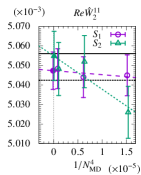
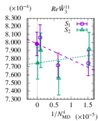
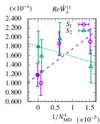
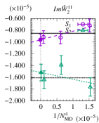
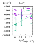
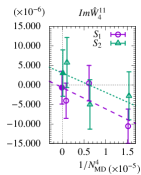
Figure 1: MD step size dependence and extrapolation for $\mathit{Re}\hat{W}^{11}_{\ell}$ (upper) and $\mathit{Im}\hat{W}^{11}_{\ell}$ (lower) at $(N,k)=(16,1)$.

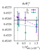
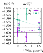
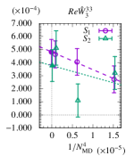
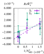
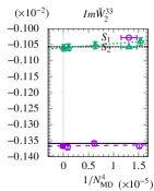
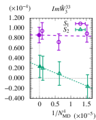
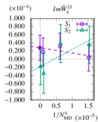
Figure 2: MD step size dependence and extrapolation for $\mathit{Re}\hat{W}^{33}_{\ell}$ (upper) and $\mathit{Im}\hat{W}^{33}_{\ell}$ (lower) at $(N,k)=(16,1)$.

3.1 Comparison with analytic calculations

As mentioned earlier the presence of the twist breaks part of the symmetries of the standard lattice symmetries with periodic boundary conditions. In particular, part of the cubic group is broken. This translates into a dependence of the coefficients of the Wilson loop perturbative expansion on the plane in which the Wilson loop lies. Due to the remaining symmetry for our choice of twist, there are two sets of planes which we label as $S_{1}=\{(\mu,\nu):(1,2),(2,3),(3,4),(4,1)\}$ and $S_{2}=\{(\mu,\nu):(1,3),(2,4)\}$ Perez:2017jyq , such that the results for all $\mu-\nu$ planes contained in each $S_{i}$ should be the same. The results for all planes in $S_{1}$ need not be equal to those contained in $S_{2}$. To increase the statistics we can average all the planes within each set.

Our results for $\hat{W}^{11}_{\ell}$ and $\hat{W}^{33}_{\ell}$ at $(N,k)=(16,1)$ are shown in figures 1 and 2, respectively. The mean values are plotted as a function of $1/N_{\mathrm{MD}}^{4}$ and extrapolated linearly to vanishing step size. The linear dependence in this variable is the expectation for our 4th order leapfrog scheme for the MD integrator, and our data are consistent with this expectation. The data for the $S_{1}$ and $S_{2}$ planes are plotted and extrapolated separately (purple dashed : $S_{1}$, green dotted : $S_{2}$). The analytic results, depicted by horizontal lines in the same plots, only predict differences among planes for $\hat{W}_{2}$. At all orders, the cubic symmetry breaking in the real parts is found to be small and of the order of the errors of our calculation. As mentioned earlier the imaginary parts beyond the leading order are non-zero and different for the two families of planes. Our results reproduce both features and match nicely with the analytic results for the first two coefficients.

	$S_{1}$			$S_{2}$
	Analytic	NSPT	$\chi^{2}/\mathrm{DoF}$	Analytic	NSPT	$\chi^{2}/\mathrm{DoF}$
$Re\hat{W}_{1}^{11}$	$0.124\,511\,72$	$0.124\,522\,3$ p m 0.0000093	$1.0$	$=S_{1}$	$0.124\,512$ p m 0.000012	$0.068$
$Re\hat{W}_{1}^{22}$	$0.328\,125\,00$	$0.328\,138$ p m 0.000037	$0.60$	$=S_{1}$	$0.328\,096$ p m 0.000045	$4.4$
$Re\hat{W}_{1}^{33}$	$0.452\,636\,72$	$0.452\,662$ p m 0.000050	$0.35$	$=S_{1}$	$0.452\,601$ p m 0.000057	$1.8$
$Re\hat{W}_{2}^{11}$	$0.005\,055\,99$	$0.005\,047\,3$ p m 0.0000096	$0.057$	$0.005\,042\,42$	$0.005\,055$ p m 0.000013	$0.52$
$Re\hat{W}_{2}^{22}$	$-0.014\,673\,13$	$-0.014\,691$ p m 0.000043	$1.0$	$-0.014\,736\,99$	$-0.014\,698$ p m 0.000056	$4.1$
$Re\hat{W}_{2}^{33}$	$-0.045\,993\,08$	$-0.045\,988$ p m 0.000062	$2.3$	$-0.045\,920\,18$	$-0.045\,817$ p m 0.000074	$2.9$
$Re\hat{W}_{2}^{44}$	$0.158\,384\,33$	$0.158\,400$ p m 0.000045	9.4 $\times 10^{-8}$	$0.157\,896\,05$	$0.157\,894$ p m 0.000045	$0.023$
$Re\hat{W}_{3}^{11}$		$0.000\,798$ p m 0.000014	$1.4$		$0.000\,775$ p m 0.000020	$1.8$
$Re\hat{W}_{3}^{22}$		$0.000\,114$ p m 0.000069	$0.38$		$0.000\,051$ p m 0.000089	$2.3$
$Re\hat{W}_{3}^{33}$		$0.000\,481$ p m 0.000096	$0.010$		$0.000\,38$ p m 0.00012	$4.4$
$Re\hat{W}_{3}^{44}$		$-0.023\,093$ p m 0.000053	$0.050$		$-0.022\,910$ p m 0.000056	$1.2$
$Re\hat{W}_{4}^{11}$		$0.000\,118$ p m 0.000025	$2.7$		$0.000\,179$ p m 0.000033	$1.1$
$Re\hat{W}_{4}^{22}$		$-0.000\,13$ p m 0.00012	$2.5$		$0.000\,10$ p m 0.00015	$1.2$
$Re\hat{W}_{4}^{33}$		$-0.000\,34$ p m 0.00016	$0.51$		$-0.000\,18$ p m 0.00020	$3.2$
$Re\hat{W}_{4}^{44}$		$0.000\,837$ p m 0.000083	$0.72$		$0.000\,775$ p m 0.000093	$0.83$
$|Im\hat{W}_{2}^{11}|$	$0.000\,008\,51$	$0.000\,009\,62$ p m 0.00000100	$0.37$	$0.000\,016\,08$	$0.000\,015\,2$ p m 0.0000014	$2.3$
$|Im\hat{W}_{2}^{22}|$	$0.000\,208\,33$	$0.000\,208\,4$ p m 0.0000036	$0.90$	$0.000\,044\,85$	$0.000\,050\,7$ p m 0.0000051	$1.4$
$|Im\hat{W}_{2}^{33}|$	$0.001\,358\,65$	$0.001\,366\,6$ p m 0.0000074	$1.1$	$0.001\,056\,71$	$0.001\,060$ p m 0.000010	$0.000\,16$
$|Im\hat{W}_{3}^{11}|$		$0.000\,000\,4$ p m 0.0000021	$0.23$		$0.000\,004\,6$ p m 0.0000031	$0.13$
$|Im\hat{W}_{3}^{22}|$		$0.000\,002\,3$ p m 0.0000071	$1.7$		$0.000\,016$ p m 0.000010	$0.075$
$|Im\hat{W}_{3}^{33}|$		$0.000\,086$ p m 0.000015	$0.99$		$0.000\,024$ p m 0.000022	$0.011$
$|Im\hat{W}_{3}^{44}|$		$0.000\,000\,7$ p m 0.0000012	$0.18$		$0.000\,001\,2$ p m 0.0000017	$0.035$
$|Im\hat{W}_{4}^{11}|$		$0.000\,000\,7$ p m 0.0000042	$1.5$		$0.000\,003\,0$ p m 0.0000059	$0.94$
$|Im\hat{W}_{4}^{22}|$		$0.000\,004$ p m 0.000013	$0.24$		$0.000\,017$ p m 0.000019	$0.000\,84$
$|Im\hat{W}_{4}^{33}|$		$0.000\,028$ p m 0.000031	$0.22$		$0.000\,018$ p m 0.000045	$0.65$
$|Im\hat{W}_{4}^{44}|$		$0.000\,005\,2$ p m 0.0000036	$0.20$		$0.000\,002\,8$ p m 0.0000051	$2.6$

Table 2: Perturbative coefficients for Wilson loops on $S_{1},S_{2}$ planes. (SU(16),$k=1$)

	$S_{1}$			$S_{2}$
	Analytic	NSPT	$\chi^{2}/\mathrm{DoF}$	Analytic	NSPT	$\chi^{2}/\mathrm{DoF}$
$Re\hat{W}_{1}^{11}$	$0.124\,947\,94$	$0.124\,954\,2$ p m 0.0000053	$0.030$	$=S_{1}$	$0.124\,957\,9$ p m 0.0000065	$0.038$
$Re\hat{W}_{1}^{22}$	$0.341\,345\,68$	$0.341\,372$ p m 0.000021	$2.7$	$=S_{1}$	$0.341\,395$ p m 0.000025	$0.78$
$Re\hat{W}_{1}^{33}$	$0.570\,101\,77$	$0.570\,171$ p m 0.000046	$0.34$	$=S_{1}$	$0.570\,128$ p m 0.000054	$1.6$
$Re\hat{W}_{1}^{44}$	$0.789\,492\,99$	$0.789\,596$ p m 0.000071	$0.44$	$=S_{1}$	$0.789\,543$ p m 0.000082	$1.1$
$Re\hat{W}_{2}^{11}$	$0.005\,101\,03$	$0.005\,103\,7$ p m 0.0000061	$7.6$	$0.005\,100\,26$	$0.005\,101\,2$ p m 0.0000077	$0.22$
$Re\hat{W}_{2}^{22}$	$-0.016\,678\,06$	$-0.016\,682$ p m 0.000026	$0.013$	$-0.016\,680\,76$	$-0.016\,677$ p m 0.000033	$1.0$
$Re\hat{W}_{2}^{33}$	$-0.088\,228\,03$	$-0.088\,249$ p m 0.000061	$0.0043$	$-0.088\,235\,09$	$-0.088\,183$ p m 0.000074	$0.018$
$Re\hat{W}_{2}^{44}$	$-0.206\,182\,50$	$-0.206\,18$ p m 0.00010	$0.12$	$-0.206\,240\,12$	$-0.206\,13$ p m 0.00012	$0.034$
$Re\hat{W}_{3}^{11}$		$0.000\,774\,1$ p m 0.0000096	$1.1$		$0.000\,784$ p m 0.000013	$1.3$
$Re\hat{W}_{3}^{22}$		$-0.000\,029$ p m 0.000043	$0.021$		$-0.000\,107$ p m 0.000054	$2.6$
$Re\hat{W}_{3}^{33}$		$0.002\,795$ p m 0.000095	$0.068$		$0.002\,64$ p m 0.00012	$0.064$
$Re\hat{W}_{3}^{44}$		$0.019\,48$ p m 0.00016	$0.0025$		$0.019\,24$ p m 0.00019	$0.0023$
$Re\hat{W}_{4}^{11}$		$0.000\,177$ p m 0.000018	$0.48$		$0.000\,171$ p m 0.000024	$0.64$
$Re\hat{W}_{4}^{22}$		$0.000\,128$ p m 0.000077	$0.044$		$0.000\,254$ p m 0.000097	$0.22$
$Re\hat{W}_{4}^{33}$		$0.000\,21$ p m 0.00017	$0.019$		$0.000\,55$ p m 0.00021	$0.43$
$Re\hat{W}_{4}^{44}$		$-0.000\,17$ p m 0.00027	$0.045$		$0.000\,38$ p m 0.00034	$0.28$
$|Im\hat{W}_{2}^{11}|$	$0.000\,000\,29$	$0.000\,000\,55$ p m 0.00000059	$0.31$	$0.000\,001\,02$	$0.000\,000\,01$ p m 0.00000085	$1.7$
$|Im\hat{W}_{2}^{22}|$	$0.000\,014\,24$	$0.000\,013\,5$ p m 0.0000027	$0.32$	$0.000\,001\,99$	$0.000\,004\,1$ p m 0.0000038	$0.35$
$|Im\hat{W}_{2}^{33}|$	$0.000\,018\,24$	$0.000\,016\,4$ p m 0.0000063	$1.3$	$0.000\,064\,97$	$0.000\,054\,4$ p m 0.0000089	$0.097$
$|Im\hat{W}_{2}^{44}|$	$0.000\,383\,14$	$0.000\,386$ p m 0.000011	$1.2$	$0.000\,447\,56$	$0.000\,438$ p m 0.000017	$0.14$
$|Im\hat{W}_{3}^{11}|$		$0.000\,000\,1$ p m 0.0000013	$0.0017$		$0.000\,002\,2$ p m 0.0000020	$1.5$
$|Im\hat{W}_{3}^{22}|$		$0.000\,005\,9$ p m 0.0000056	$3.9$		$0.000\,004\,4$ p m 0.0000076	$0.75$
$|Im\hat{W}_{3}^{33}|$		$0.000\,018$ p m 0.000014	$1.4$		$0.000\,031$ p m 0.000018	$0.67$
$|Im\hat{W}_{3}^{44}|$		$0.000\,102$ p m 0.000025	$0.61$		$0.000\,088$ p m 0.000037	$0.053$
$|Im\hat{W}_{4}^{11}|$		$0.000\,000\,8$ p m 0.0000026	$0.044$		$0.000\,003\,5$ p m 0.0000039	$0.22$
$|Im\hat{W}_{4}^{22}|$		$0.000\,003$ p m 0.000011	$2.2$		$0.000\,008$ p m 0.000015	$0.39$
$|Im\hat{W}_{4}^{33}|$		$0.000\,056$ p m 0.000029	$0.25$		$0.000\,068$ p m 0.000039	$1.8$
$|Im\hat{W}_{4}^{44}|$		$0.000\,108$ p m 0.000053	$0.86$		$0.000\,021$ p m 0.000079	$0.15$

Table 3: Perturbative coefficients for Wilson loops on $S_{1},S_{2}$ planes. (SU(49),$k=2$)

All our results for $(N,k)=(16,1)$ and $(49,2)$, extrapolated linearly in $1/N_{\mathrm{MD}}^{4}$ to zero, are collected in Tables 2 and 3. We also tabulate the analytic values from ref. Perez:2017jyq and $\chi^{2}/\mathrm{DoF}$ from the extrapolating fit. The violation of CP and cubic invariance due to the twist is well seen for the $N=16$ case at the two loop level and the differences between $S_{1}$ and $S_{2}$ averages are consistent with the analytic values. For the $(N,k)=(49,2)$ case, the results of our NSPT analysis are also consistent with analytic values. However, the violation of CP and cubic invariance is too small to be seen in comparison with the statistical errors. Since the violation of CP and cubic invariance disappears in the large $N$ limit, we conclude that in practice one would not be able see any effect of this symmetry breaking for even larger values of $N$. Hence, hereafter, we show the coefficients averaged over all $\mu$–$\nu$ planes ($S=S_{1}+S_{2}$) in order to study the $k$ dependence and $N$ dependence. We emphasize the small errors of our coefficient determinations, typically of order $10^{-5}$. This gives about 3 to 5 significant digits in some determinations.

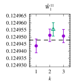
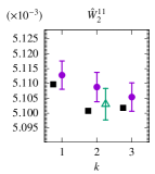
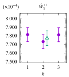
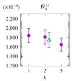
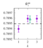
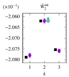
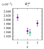
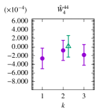
Figure 3: $k$ dependence for $\hat{W}_{\ell}^{11}$ and $\hat{W}_{\ell}^{44}$ at $N=49$. Open triangles show the results extrapolated to $1/N_{\mathrm{MD}}\to 0$ and the other values are at $N_{\mathrm{MD}}=32$. Dashed line in $\hat{W}^{RR}_{1}$ and filled squares in $\hat{W}^{RR}_{2}$ are the analytic values Perez:2017jyq ; privcomm .

We next investigate the dependence on the flux parameter $k$ at $N=49$. For that purpose we studied the $k=1$ and $k=3$ results at fixed value of $N_{\mathrm{MD}}=32$. The results for the coefficients for the plaquette and $4\times 4$ Wilson loop are displayed in figure 3. The results for $k=2$ are given both at $N_{\mathrm{MD}}=32$ as well as extrapolated $1/N_{\mathrm{MD}}\to 0$ (open triangles). From the data we conclude that $N_{\mathrm{MD}}=32$ is sufficient for the current analysis as the statistical error and the systematic error from the finite MD time step are comparable. The horizontal dash lines in $\hat{W}^{RR}_{1}$ and the filled squares in $\hat{W}^{RR}_{2}$ correspond to the analytic values. For the plaquette, the observed $k$-dependence is compatible with statistical errors. As expected, the differences are small but well beyond statistical errors for the $4\times 4$ loop. This is also the case for the third order coefficient $\hat{W}^{RR}_{3}$ for which we have no analytic results. Anyhow, no dramatic $k$ dependence is seen for the third and fourth order coefficients.

Our results averaged over all planes are displayed in table 4. The choice of values $(N,k)=(16,1),(49,2),(121,3)$ are selected so as to keep $k/\hat{L}$ at $\sim 0.27$ ($k/\hat{L}=1/4,2/7,3/11$ for each data set). The results at the one and two-loop level are consistent with the analytic values within two standard deviations. We also display (NPT fit) an estimate of the three-loop coefficients for $N=16$ and $49$ obtained by fitting nonperturbative expectation values to a third order polynomial in $\lambda$ with the first coefficients fixed to the analytic values Perez:2017jyq . The results are roughly consistent with our NSPT determinations, which are expected to be more reliable.

SU(16), $k=1$	$\ell=1$	$\ell=2$	$\ell=3$	$\ell=4$
$\hat{W}^{11}_{\ell}$	$0.124\,518\,8$ p m 0.0000086	$0.005\,049\,7$ p m 0.0000084	$0.000\,791$ p m 0.000012	$0.000\,138$ p m 0.000021
$\hat{W}^{22}_{\ell}$	$0.328\,123$ p m 0.000034	$-0.014\,695$ p m 0.000038	$0.000\,094$ p m 0.000061	$-0.000\,05$ p m 0.00011
$\hat{W}^{33}_{\ell}$	$0.452\,642$ p m 0.000047	$-0.045\,930$ p m 0.000056	$0.000\,448$ p m 0.000088	$-0.000\,29$ p m 0.00015
$\hat{W}^{44}_{\ell}$	$0.0$	$0.158\,232$ p m 0.000044	$-0.023\,032$ p m 0.000051	$0.000\,816$ p m 0.000079
	PT Analytic	PT Analytic	NPT Fit
$\hat{W}^{11}_{\ell}$	$0.124\,511\,72$	$0.005\,051\,46$	$0.000\,826(36)$
$\hat{W}^{22}_{\ell}$	$0.328\,125\,00$	$-0.014\,694\,41$	$0.000\,04(12)$
$\hat{W}^{33}_{\ell}$	$0.452\,636\,72$	$-0.045\,968\,78$	$0.000\,34(16)$
$\hat{W}^{44}_{\ell}$	$0.0$	$0.158\,221\,57$	$-0.022\,88(6)$
SU(49), $k=2$	$\ell=1$	$\ell=2$	$\ell=3$	$\ell=4$
$\hat{W}^{11}_{\ell}$	$0.124\,955\,5$ p m 0.0000047	$0.005\,103\,0$ p m 0.0000053	$0.000\,777\,4$ p m 0.0000085	$0.000\,175$ p m 0.000016
$\hat{W}^{22}_{\ell}$	$0.341\,380$ p m 0.000019	$-0.016\,680$ p m 0.000024	$-0.000\,055$ p m 0.000040	$0.000\,171$ p m 0.000071
$\hat{W}^{33}_{\ell}$	$0.570\,156$ p m 0.000042	$-0.088\,227$ p m 0.000055	$0.002\,743$ p m 0.000084	$0.000\,33$ p m 0.00015
$\hat{W}^{44}_{\ell}$	$0.789\,578$ p m 0.000066	$-0.206\,163$ p m 0.000097	$0.019\,40$ p m 0.00014	$0.000\,01$ p m 0.00025
	PT Analytic	PT Analytic	NPT Fit
$\hat{W}^{11}_{\ell}$	$0.124\,947\,94$	$0.005\,100\,77$	$0.000\,883(9)$
$\hat{W}^{22}_{\ell}$	$0.341\,345\,68$	$-0.016\,678\,96$	$0.000\,086(36)$
$\hat{W}^{33}_{\ell}$	$0.570\,101\,77$	$-0.088\,230\,39$	$0.002\,93(5)$
$\hat{W}^{44}_{\ell}$	$0.789\,492\,99$	$-0.206\,201\,71$	$0.019\,59(7)$
SU(121), $k=3$	$\ell=1$	$\ell=2$	$\ell=3$	$\ell=4$
$\hat{W}^{11}_{\ell}$	$0.124\,988\,7$ p m 0.0000037	$0.005\,103\,6$ p m 0.0000041	$0.000\,788\,4$ p m 0.0000069	$0.000\,156$ p m 0.000012
$\hat{W}^{22}_{\ell}$	$0.342\,179$ p m 0.000015	$-0.016\,760$ p m 0.000019	$-0.000\,030$ p m 0.000032	$0.000\,020$ p m 0.000055
$\hat{W}^{33}_{\ell}$	$0.575\,489$ p m 0.000034	$-0.090\,700$ p m 0.000043	$0.002\,995$ p m 0.000068	$0.000\,03$ p m 0.00012
$\hat{W}^{44}_{\ell}$	$0.812\,537$ p m 0.000056	$-0.220\,758$ p m 0.000080	$0.022\,06$ p m 0.00012	$-0.000\,39$ p m 0.00021
$\hat{W}^{55}_{\ell}$	$1.049\,316$ p m 0.000088	$-0.407\,28$ p m 0.00014	$0.070\,62$ p m 0.00021	$-0.004\,59$ p m 0.00038
$\hat{W}^{66}_{\ell}$	$1.281\,72$ p m 0.00012	$-0.645\,07$ p m 0.00021	$0.160\,12$ p m 0.00033	$-0.019\,33$ p m 0.00057
	PT Analytic	PT Analytic privcomm
$\hat{W}^{11}_{\ell}$	$0.124\,991\,46$	$0.005\,105\,92$
$\hat{W}^{22}_{\ell}$	$0.342\,183\,32$	$-0.016\,797\,72$
$\hat{W}^{33}_{\ell}$	$0.575\,499\,81$	$-0.090\,734\,26$
$\hat{W}^{44}_{\ell}$	$0.812\,550\,00$	$-0.220\,851\,02$
$\hat{W}^{55}_{\ell}$	$1.049\,336\,25$	$-0.407\,409\,49$
$\hat{W}^{66}_{\ell}$	$1.281\,751\,42$	$-0.645\,311\,88$

Table 4: Perturbative coefficients for Wilson loops ($1/N_{\mathrm{MD}}\to 0$ extrapolated). Data in PT Analytic are obtained analytically and data in NPT Fit are obtained by fitting the non-perturbative data with a polynomial of $\lambda$ Perez:2017jyq .

Since the main interest of the TEK model is its large $N$ limit, which coincides with Yang-Mills at infinite $N$ and infinite volume, we give the infinite $N$ extrapolation of our results. As mentioned previously finite $N$ corrections are expected to grow for large values of $R/\hat{L}$. Thus, we exclude the data of $(N,k)=(16,1)$ and base our analysis on $(N,k)=(121,3)$ and $(49,2)$ only and assuming a $1/N^{2}$ dependence of the coefficients. The results are displayed in figure 4 and the numerical values of the extrapolated coefficients are tabulated in table 5. In the figure we only show the plaquette and $4\times 4$ Wilson loop up to three-loop order. The error includes only the statistical one. The values extrapolated to $N\to\infty$ are shown as filled circles, while the horizontal solid lines are the corresponding analytic values DiGiacomo:1981lcx ; Alles:1993dn ; Alles:1998is ; Perez:2017jyq ; privcomm . We see a reasonable good agreement within errors. The deviations for the $4\times 4$ loop might include also a systematic error due to the relatively large values of $4/\hat{L}$. For a more precise control of the systematic errors in the extrapolated results it would be necessary to have at least 3 sufficiently large values of $N$, which is left out of this exploratory work.

$N\to\infty$	$\ell=1$	$\ell=2$	$\ell=3$
$\hat{W}^{11}_{\ell}$	$0.124\,999\,9$ p m 0.0000054	$0.005\,113\,4$ p m 0.0000059	$0.000\,790\,5$ p m 0.0000099
$\hat{W}^{22}_{\ell}$	$0.342\,336$ p m 0.000021	$-0.016\,775$ p m 0.000027	$-0.000\,025$ p m 0.000046
$\hat{W}^{33}_{\ell}$	$0.576\,534$ p m 0.000049	$-0.091\,185$ p m 0.000063	$0.003\,044$ p m 0.000098
$\hat{W}^{44}_{\ell}$	$0.817\,004$ p m 0.000080	$-0.223\,62$ p m 0.00011	$0.022\,59$ p m 0.00017
	PT Analytic	PT Analytic	PT Analytic
$\hat{W}^{11}_{\ell}$	$0.125\,000\,00$	$0.005\,106\,929\,7$	$0.000\,794\,223$ p m 0.000000019
$\hat{W}^{22}_{\ell}$	$0.342\,327\,88$	$-0.016\,814$
$\hat{W}^{33}_{\ell}$	$0.576\,298\,27$	$-0.091\,07$
$\hat{W}^{44}_{\ell}$	$0.815\,370\,98$	$-0.222\,87$

Table 5: Perturbative coefficients for $\hat{W}^{RR}_{\ell}$ in $N\to\infty$. Values in PT Analytic for $\hat{W}^{11}_{\ell}$ are $N\to\infty$ limit of results from lattice $\mathrm{SU}(N)$ gauge theory with Wilson gauge action Alles:1998is .

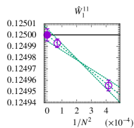
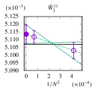
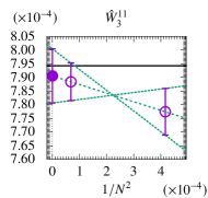
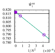
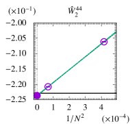
Figure 4: $N\to\infty$ limit of perturbative coefficients using data from $(N,k)=(49,2)$ and $(121,3)$ (upper : plaquette, lower : $4\times 4$ Wilson loop).

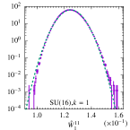
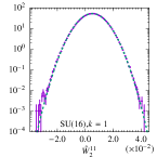
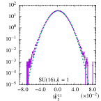
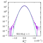
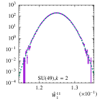
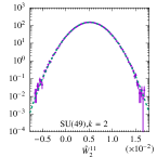
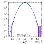
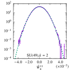
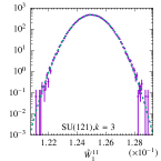
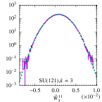
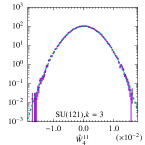
Figure 5: Histogram of $\hat{W}_{\ell}^{11}$ at $\ell=1,2,3,4$ from left to right (top row: $N=16$, middle: $N=49$, bottom : $N=121$). Results from $N_{\mathrm{MD}}=32$.

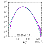
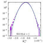
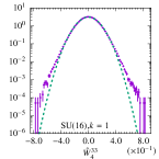
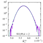
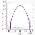
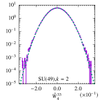
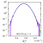
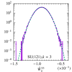
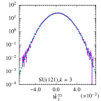
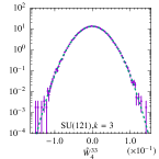
Figure 6: Same as figure 5, but for $\hat{W}_{\ell}^{33}$.

3.2 Analysis of the distribution

For the purpose of determining the statistical requirements involved in a precise determination of the perturbative coefficients we performed an analysis of the probability distribution of the corresponding NSPT estimates. As a quantitative measure we computed the cumulants up to the 5th cumulant. The $N$ dependence of the variance (second cumulant) is important since the statistical error at fixed statistics is proportional to the square root of this variance. The non-zero value of higher order cumulants measures the deviation from the normal distribution. This is of practical importance since, as seen in ref. Alfieri:2000ce , the distribution for perturbative coefficients at higher order in NSPT could show strong deviations from a normal distribution, the so-called “Pepe effect”. We show the histograms for $\hat{W}^{11}_{\ell}$ and $\hat{W}^{33}_{\ell}$ in figures 5 and 6, respectively. We have fixed $N_{\mathrm{MD}}=32$ for better comparison. The distributions are plotted in logarithmic scale for which the normal distribution corresponds to a parabola. The dotted lines are the best fit to a normal distribution. One can see deviations in the tail for some plots for $N=16$, but it disappears for larger $N$. Hence, the problem of “Pepe effect” is absent in the TEK model for sufficiently large $N$, similarly to what happens for pure SU(3) lattice gauge theory. Since the 3rd–5th cumulants have minor effect or are not detectable on the distribution, we focus on the variance only in the following analysis.

We have studied the dependence of the variance of $\hat{W}_{\ell}^{RR}$ on $R$, $\ell$ and $N$. Notice that we can also use the results for half-integer $\ell$ in this analysis. The $R$ dependence is illustrated in figure 7, and is seen to go linearly with $R^{4}$. On the other hand the dependence on $j=2\ell$, displayed in figure 8 shows an exponential behaviour for sufficiently large $j$. Altogether, an ansatz of the form

$$\sigma^{2}(N,j) =\dfrac{cR^{4}}{N^{2}}\left(2-\dfrac{1}{\sqrt{N}}\right)^{2\ell},$$ (159)

with $c=0.0013$ (solid lines in these figures) describes our data quite well. For large $N$ this corresponds to a dependence on the ratio of the loop size with respect to the effective size of the box $R/\hat{L}$ to the fourth power, similar to the observed subleading corrections in perturbation theory.

The $1/N^{2}$ dependence of the variance follows from the perturbative realization of factorization $\langle W^{2}\rangle=\langle W\rangle^{2}+O(1/N^{2})$. Similar arguments lead to the prediction that the $p$-th cumulant scales as $O(1/N^{2p-2})$. This by itself explains why the distribution tends to normal at large $N$. We cannot check this behaviour of the higher cumulants since their values are too small.

The exponential dependence of the variance on the order $4^{\ell}$ coincides precisely with the characteristic growth in the number of planar diagrams Brezin:1977sv ; Koplik:1977pf ; Marino:2012zq , given by the Catalan number. In the absence of renormalons, a similar growth is also expected for the mean values $\hat{W}_{\ell}$, but it is hard to check this behaviour with our results reaching only up to order $\ell=4$. Indeed, as observed in ref. Bali:2014fea , extremely large order perturbative coefficients are needed to detect the expected factorial behavior for the pure SU(3) lattice gauge theory. Hence, it would be interesting to extend our results to higher order to explore this point. The computational requirements will be studied in the next subsection.

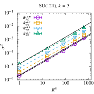
Figure 7: The loop size dependence of the variance $\sigma^{2}$ for $\hat{W}_{j/2}^{RR}$ ($N_{\mathrm{MD}}=32$, $j\geq 5$ and SU(121), $k=3$). The dotted line shows the result of a fit. Solid lines represent the ansatz eq. (159) with $\ell=5/2$ and $8/2$.

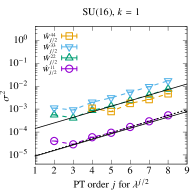
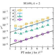
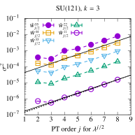
Figure 8: Variance $\sigma^{2}$ for $\hat{W}_{j/2}^{RR}$ at $N_{\mathrm{MD}}=32$. Dotted lines are the results of a fit to the $j\geq 5$ data. Solid lines represent the ansatz eq. (159) with $R=1$ for all $\mathrm{SU}(N)$ and with $R=2,3,4$ for $N=16,49,121$, respectively.

4 Estimate of the computational cost at high order and large $N$

Here we will evaluate the computer requirements to extend our calculation $\hat{W}_{\ell}$ up to order $\ell=N_{\mathrm{trunc}}/2$. The precision in the determination is proportional to the standard deviation of the corresponding probability distribution. Hence, if we want to keep this precision fixed our data sample should grow with the square, the variance. We previously estimated that for each sample point the computational cost goes as $O(N^{7/2}N_{\mathrm{trunc}}^{3})$ for the MD part and as $O(N^{3}N_{\mathrm{trunc}}^{4})$ for the reunitarization part. Using eq. (159), we can then give an estimate of the total computational cost as follows:

$$\mathrm{[Cost]} \propto(N^{7/2}N_{\mathrm{trunc}}^{3})\times\sigma^{2}(N,N_{\mathrm{trunc}})\propto N^{3/2}N_{\mathrm{trunc}}^{3}\left(2-\dfrac{1}{\sqrt{N}}\right)^{N_{\mathrm{trunc}}},$$ (160)

or

$$\mathrm{[Cost]} \propto(N^{3}N_{\mathrm{trunc}}^{4})\times\sigma^{2}(N,N_{\mathrm{trunc}})\propto NN_{\mathrm{trunc}}^{4}\left(2-\dfrac{1}{\sqrt{N}}\right)^{N_{\mathrm{trunc}}}.$$ (161)

This estimate can be reduced by improving the algorithm. To obtain perturbative coefficients at very higher order, the exponential scaling behaviour, $2^{N_{\mathrm{trunc}}}$, has to be relaxed by reducing the variance using a method such as a kind of reweighting method in NSPT. Furthermore, the factor $N_{\mathrm{trunc}}^{4}$ comes from our implementation of the reunitarization algorithm, for which a better algorithm could be applicable. One possibility is to use the perturbative Gram-Schmidt algorithm for the reorthogonalization followed by the perturbative subtraction of the U(1) phase. The estimation of the U(1) phase still requires the perturbative trace-log computation whose cost is of $O(N_{\mathrm{trunc}}^{3})$. At least one can reduce the factor from $N_{\mathrm{trunc}}^{4}$ to $N_{\mathrm{trunc}}^{3}$. In that case eq. (160) would dominate the total cost.

The cost of $O(N_{\mathrm{trunc}}^{2})$ in the convolutional product of two series could be ameliorated by using the fast Fourier transformation (FFT) algorithm, which reduces the cost to $O(N_{\mathrm{trunc}}\log N_{\mathrm{trunc}})$. Improvement in this direction can be used in future studies.

5 Summary

In this paper we have developed and applied an HMD-based NSPT algorithm to compute the perturbative expansion of Wilson loops in the TEK model. At large $N$ these coefficients coincide with those of large volume Yang-Mills theory, hence their interest. The low order coefficients are very precise and match with the values obtained by the analytic calculation of ref. Perez:2017jyq . We have been able to extend the perturbative series two more orders, up to $O(\lambda^{4})$.

We also studied the statistical properties of the coefficients in NSPT. We found that their distribution tends to normal at large $N$ and there is no Pepe effect. Furthermore, we have determined the dependence of the corresponding variance on $N$ and the order of perturbation theory. This has allowed us to estimate the computational requirements necessary to extend our results to higher orders. This would allow extending studies of the type described in ref. Marino:2012zq to Yang-Mills theory in the limit of infinite number of colours.

Appendix A Perturbative matrix functions

In this appendix we describe the details of evaluating the perturbative coefficients of a matrix function with a perturbative series as the argument. After introducing the generic algorithm for perturbative matrix functions, we explain the cases with matrix exponential and matrix logarithm explicitly.

We consider a matrix function $f(F)$ whose argument $F$ is a matrix. We assume that $f(F)$ has the following Taylor expansion form:

$$f(F) =\sum_{k=0}^{\infty}c_{k}F^{k}.$$ (162)

We also assume that the perturbative expansion of $F$ is

$$F =\sum_{k=1}^{\infty}g^{k}F^{(k)},$$ (163)

where $g$ is the coupling constant and $F^{(k)}$ are the coefficient matrices. Note that the leading term of $F$ is $O(g)$. We truncate the perturbative expansion at $N_{\mathrm{trunc}}$-th order.

$$F =\sum_{k=1}^{N_{\mathrm{trunc}}}g^{k}F^{(k)}.$$ (164)

The perturbative expansion of $f(F)$ with eq. (164) is also truncated at $N_{\mathrm{trunc}}$ as

$$f(\sum_{k=1}^{N_{\mathrm{trunc}}}g^{k}F^{(k)}) =c_{0}I+\sum^{N_{\mathrm{trunc}}}_{k=1}g^{k}\left[f(F)\right]^{(k)}.$$ (165)

We would like to know the coefficient $\left[f(F)\right]^{(k)}$ in terms of $c_{k}$’s and $F^{(k)}$’s. A recursion relation to evaluate the coefficient $\left[f(F)\right]^{(k)}$ can be obtained by expanding the Horner’s method for polynomials as follows.

As $F$ is truncated at $N_{\mathrm{trunc}}$-th order, the Taylor expansion is also truncated at $N_{\mathrm{trunc}}$-th order,

$$f(F) \simeq G=\sum_{k=0}^{N_{\mathrm{trunc}}}c_{k}F^{k},$$ (166)

where the matrix $G$ is introduced for the truncated form. $G$ can be evaluated via the Horner’s method:

$$G=f(F) =c_{0}+c_{1}F+c_{2}F^{2}+\cdots+c_{N_{\mathrm{trunc}}}F^{N_{\mathrm{trunc}}}$$

$$=c_{0}\left[I+d_{1}F\left[I+d_{2}F\left[I+\cdots\left[I+d_{N_{\mathrm{trunc}}}F\right]\cdots\right]\right]\right],$$ (167)

$$d_{j} \equiv c_{j}/c_{j-1}.$$ (168)

This form leads to the following recursion relation:

$$G_{N} =I+d_{N_{\mathrm{trunc}}}F,$$ (169)

$$G_{j} =I+d_{j}FG_{j+1},\quad\mbox{for $j=N_{\mathrm{trunc}}-1,N_{\mathrm{trunc}}-2,\dots,2,1$},$$ (170)

$$G =c_{0}G_{1},$$ (171)

where $G_{j}$ are working area. As $F$ has the series form eq. (163), $G_{j}$ also has the series form:

$$G_{j} =I+\sum_{k=1}^{N_{\mathrm{trunc}}}g^{k}G_{j}^{(k)}.$$ (172)

Substituting the series form (164) for $F$ and (172) for $G_{j}$ into the recursion relation, we obtain

$$G_{j} =I+\sum_{k=1}^{N_{\mathrm{trunc}}}g^{k}G_{j}^{(k)}$$

$$=I+d_{j}\left(\sum_{k=1}^{N}g^{k}F^{(k)}\right)\left(I+\sum_{k=1}^{N}g^{k}G_{j+1}^{(k)}\right)$$

$$=I+d_{j}\left[\sum_{k=1}^{N_{\mathrm{trunc}}}g^{k}F^{(k)}+\sum_{k=1}^{N_{\mathrm{trunc}}}\sum_{\ell=1}^{N_{\mathrm{trunc}}}g^{k+\ell}F^{(k)}G_{j+1}^{(\ell)}\right]$$

$$=I+d_{j}\left[\sum_{k=1}^{N_{\mathrm{trunc}}}g^{k}F^{(k)}+\sum_{k=2}^{N_{\mathrm{trunc}}}g^{k}\sum_{\ell=1}^{k-1}F^{(k-\ell)}G_{j+1}^{(\ell)}\right].$$ (173)

Here we discard higher order terms $O(g^{k})$ with $k>N_{\mathrm{trunc}}$.

Consequently the perturbative coefficient $[f(F)]^{(k)}$ of $f(F)$ can be obtained as algorithm 3. The computational cost scales with $N_{\mathrm{trunc}}^{3}$.

Algorithm 3 Recursion algorithm for the perturbative expansion of a matrix function $f(F)$. The maximum order $N_{\mathrm{trunc}}$ of expansion is fixed. $G^{(k)}$ is the perturbative coefficient $[f(F)]^{(k)}$.

1:  for $k=1$ to $N_{\mathrm{trunc}}$ do

2:     $G_{N_{\mathrm{trunc}}}^{(k)}=d_{N_{\mathrm{trunc}}}F^{(k)}$

3:  end for

4:  for $j=N_{\mathrm{trunc}}-1$ to $1$ do

5:     for $k=N_{\mathrm{trunc}}$ to $1$ do

6:        $G_{j}^{(k)}=d_{j}\left[F^{(k)}+\sum_{\ell=1}^{k-1}F^{(k-\ell)}G_{j+1}^{(\ell)}\right]$

7:     end for

8:  end for

9:  for $k=1$ to $N_{\mathrm{trunc}}$ do

10:     $G^{(k)}=c_{0}G_{1}^{(k)}$

11:  end for

A.1 Matrix exponential for updating $U$

Here we consider the case of $f(F)=\exp(F)=\exp(iP\Delta\tau)$ with $P=\sum_{k=1}^{\infty}\beta^{-k/2}P^{(k)}$. The Taylor expansion for $f(F)$ is

$$f(F)=\exp(F) =I+\sum_{k=1}^{\infty}\dfrac{1}{k!}F^{k}$$

$$\exp(iP\Delta\tau) =I+\sum_{k=1}^{\infty}\dfrac{(i\Delta\tau)^{k}}{k!}P^{k}.$$ (174)

Thus the coefficients are $c_{k}=(i\Delta\tau)^{k}/{k!}$. We identify $F=P$, $F^{(k)}=P^{(k)}$, $d_{j}=i\Delta\tau/j$, and $[\exp(iP\Delta\tau)]^{(k)}=G_{1}^{(k)}$ with $g=\beta^{-1/2}$ for the recursion algorithm 3 (omitting the last step lines 9–11 as $c_{0}=1$).

A.2 Matrix logarithm for reunitarization

Next we consider the case of $f(F)=\ln(I+F)=\ln(U)$ with $U=I+\sum_{k=1}^{\infty}\beta^{-k/2}U^{(k)}=I+F$. The Taylor expansion for $f(F)$ is

$$f(F)=\ln(I+F) =\sum_{\ell=1}^{\infty}\dfrac{(-1)^{\ell+1}}{\ell}F^{\ell}.$$ (175)

Thus the coefficients are $c_{0}=0$, $c_{\ell}=(-1)^{\ell+1}/\ell$. As $F$ is expanded as $F=\sum_{k=1}^{\infty}\beta^{-k/2}U^{(k)}$, we can identify $F^{(k)}=U^{(k)}$, and $[\ln(U)]^{(k)}=G_{1}^{(k)}$ with $g=\beta^{-1/2}$ and $d_{j}=-(j-1)/j$ for the recursion algorithm 3.

Appendix B Perturbative reunitarization

Reunitarization of $U$ is applied perturbatively on $U^{(k)}$ via the perturbative expansion of the matrix logarithm:

$$A\equiv\ln[U] \Leftrightarrow U=\exp[A],$$ (176)

where $A$ should be anti-Hermitian and traceless for $U$ to be $\mathrm{SU}(N)$. From the perturbative expansion of the matrix logarithm and $A=\sum_{k=1}^{\infty}g^{k}A^{(k)}$, we have

$$\left[\ln[U]\right]^{(k)}=A^{(k)},$$ (177)

where $\left[\ln[U]\right]^{(k)}$ is described in subsection A.2. The $\mathrm{SU}(N)$ condition on the perturbative coefficients $A^{(k)}$ is

$${A^{(k)}}^{{\dagger}} =-A^{(k)},\qquad\operatorname{Tr}[A^{(k)}]=0.$$ (178)

By inspecting algorithm 3, we can find that the coefficient $\left[\ln[U]\right]^{(k)}=A^{(k)}$ has the following dependency on $U^{(k)}$:

$$A^{(1)} =U^{(1)},$$ (179)

$$A^{(k)} =U^{(k)}+X[U^{(1)},U^{(2)},\dots,U^{(k-1)}],\quad\mbox{for $1<k$},$$ (180)

where $X[U^{(1)},U^{(2)},\dots,U^{(k-1)}]\equiv\left[\ln[U]\right]^{(k)}-U^{(k)}$. Thus the $\mathrm{SU}(N)$ condition on $A^{(k)}$ can be guaranteed by applying algorithm 4 on $U^{(k)}$. The computational cost of algorithm 4 is $O(N_{\mathrm{trunc}}^{4})$.

In order to apply algorithm 4 to the TEK model, we have to reunitarize the matrix $V^{(k)}_{\mu}=U^{(k)}_{\mu}\Gamma^{{\dagger}}_{\mu}$ as the perturbative vacuum is $U^{(0)}_{\mu}=\Gamma_{\mu}$. After reunitarizing $V_{\mu}^{(k)}$, $U^{(k)}_{\mu}=\Gamma_{\mu}V^{(k)}_{\mu}$ is computed.

Algorithm 4 Perturbative reunitarization algorithm for a $\mathrm{SU}(N)$ matrix. $A$ and $B$ are working area.

1:  for $k=1$ to $N_{\mathrm{trunc}}$ do

2:     if $k=1$ then

3:        $A=U^{(1)}$

4:     else

5:        $A=U^{(k)}+X[U^{(1)},U^{(2)},\dots,U^{(k-1)}]$

6:     end if

7:     $B=\left(A-A^{{\dagger}}\right)/2$

8:     $A=B-\operatorname{Tr}[B]/N$

9:     if $k=1$ then

10:        $U^{(1)}=A^{(1)}$

11:     else

12:        $U^{(k)}=A^{(k)}-X[U^{(1)},U^{(2)},\dots,U^{(k-1)}]$

13:     end if

14:  end for

References

- (1) G. ’t Hooft, A Planar Diagram Theory for Strong Interactions, Nucl. Phys. B72 (1974) 461.
- (2) J. M. Maldacena, The Large N limit of superconformal field theories and supergravity, Int. J. Theor. Phys. 38 (1999) 1113 [hep-th/9711200].
- (3) K. G. Wilson, Confinement of Quarks, Phys. Rev. D10 (1974) 2445.
- (4) B. Lucini and M. Panero, SU(N) gauge theories at large N, Phys. Rept. 526 (2013) 93 [1210.4997].
- (5) B. Lucini, M. Teper and U. Wenger, The High temperature phase transition in SU(N) gauge theories, JHEP 01 (2004) 061 [hep-lat/0307017].
- (6) B. Lucini, M. Teper and U. Wenger, Glueballs and k-strings in SU(N) gauge theories: Calculations with improved operators, JHEP 06 (2004) 012 [hep-lat/0404008].
- (7) B. Lucini, M. Teper and U. Wenger, Properties of the deconfining phase transition in SU(N) gauge theories, JHEP 02 (2005) 033 [hep-lat/0502003].
- (8) T. Eguchi and H. Kawai, Reduction of Dynamical Degrees of Freedom in the Large N Gauge Theory, Phys. Rev. Lett. 48 (1982) 1063.
- (9) G. Bhanot, U. M. Heller and H. Neuberger, The Quenched Eguchi-Kawai Model, Phys. Lett. 113B (1982) 47.
- (10) D. J. Gross and Y. Kitazawa, A Quenched Momentum Prescription for Large N Theories, Nucl. Phys. B206 (1982) 440.
- (11) R. Narayanan and H. Neuberger, Large N reduction in continuum, Phys. Rev. Lett. 91 (2003) 081601 [hep-lat/0303023].
- (12) P. Kovtun, M. Ünsal and L. G. Yaffe, Volume independence in large N(c) QCD-like gauge theories, JHEP 06 (2007) 019 [hep-th/0702021].
- (13) M. Ünsal and L. G. Yaffe, Center-stabilized Yang-Mills theory: Confinement and large N volume independence, Phys. Rev. D78 (2008) 065035 [0803.0344].
- (14) A. González-Arroyo and M. Okawa, A Twisted Model for Large Lattice Gauge Theory, Phys. Lett. 120B (1983) 174.
- (15) A. González-Arroyo and M. Okawa, The Twisted Eguchi-Kawai Model: A Reduced Model for Large N Lattice Gauge Theory, Phys. Rev. D27 (1983) 2397.
- (16) A. González-Arroyo and M. Okawa, String Tension for Large Gauge Theory, Phys. Lett. 133B (1983) 415.
- (17) K. Fabricius and O. Haan, Numerical Analysis of the Twisted Eguchi-kawai Model in Four-dimensions, Phys. Lett. 139B (1984) 293.
- (18) A. González-Arroyo and M. Okawa, The string tension from smeared Wilson loops at large N, Phys. Lett. B718 (2013) 1524 [1206.0049].
- (19) A. González-Arroyo and M. Okawa, Testing volume independence of SU(N) pure gauge theories at large N, JHEP 12 (2014) 106 [1410.6405].
- (20) M. R. Douglas and N. A. Nekrasov, Noncommutative field theory, Rev. Mod. Phys. 73 (2001) 977 [hep-th/0106048].
- (21) A. González-Arroyo and C. P. Korthals Altes, Reduced Model for Large Continuum Field Theories, Phys. Lett. 131B (1983) 396.
- (22) A. Connes and M. A. Rieffel, Yang-Mills for noncommutative two-tori, Contemp. Math. 62 (1987) 237.
- (23) G. ’t Hooft, A Property of Electric and Magnetic Flux in Nonabelian Gauge Theories, Nucl. Phys. B153 (1979) 141.
- (24) M. García Pérez, A. González-Arroyo and M. Okawa, Perturbative contributions to Wilson loops in twisted lattice boxes and reduced models, JHEP 10 (2017) 150 [1708.00841].
- (25) G. V. Dunne and M. Ünsal, What is QFT? Resurgent trans-series, Lefschetz thimbles, and new exact saddles, PoS LATTICE2015 (2016) 010 [1511.05977].
- (26) A. Cherman, D. Dorigoni and M. Ünsal, Decoding perturbation theory using resurgence: Stokes phenomena, new saddle points and Lefschetz thimbles, JHEP 10 (2015) 056 [1403.1277].
- (27) M. Mariño, Lectures on non-perturbative effects in large gauge theories, matrix models and strings, Fortsch. Phys. 62 (2014) 455 [1206.6272].
- (28) D. J. Gross and E. Witten, Possible Third Order Phase Transition in the Large N Lattice Gauge Theory, Phys. Rev. D21 (1980) 446.
- (29) S. R. Wadia, A Study of U(N) Lattice Gauge Theory in 2-dimensions, 1212.2906.
- (30) P. V. Buividovich, G. V. Dunne and S. N. Valgushev, Complex Path Integrals and Saddles in Two-Dimensional Gauge Theory, Phys. Rev. Lett. 116 (2016) 132001 [1512.09021].
- (31) G. ’t Hooft, Can We Make Sense Out of Quantum Chromodynamics?, Subnucl. Ser. 15 (1979) 943.
- (32) M. Beneke, Renormalons, Phys. Rept. 317 (1999) 1 [hep-ph/9807443].
- (33) F. Di Renzo, G. Marchesini, P. Marenzoni and E. Onofri, Lattice perturbation theory by Langevin dynamics, hep-lat/9308006.
- (34) F. Di Renzo, G. Marchesini, P. Marenzoni and E. Onofri, Lattice perturbation theory on the computer, Nucl. Phys. Proc. Suppl. 34 (1994) 795.
- (35) F. Di Renzo, E. Onofri, G. Marchesini and P. Marenzoni, Four loop result in SU(3) lattice gauge theory by a stochastic method: Lattice correction to the condensate, Nucl. Phys. B426 (1994) 675 [hep-lat/9405019].
- (36) F. Di Renzo, E. Onofri and G. Marchesini, Renormalons from eight loop expansion of the gluon condensate in lattice gauge theory, Nucl. Phys. B457 (1995) 202 [hep-th/9502095].
- (37) G. Burgio, F. Di Renzo, G. Marchesini and E. Onofri, contribution to the condensate in lattice gauge theory, Phys. Lett. B422 (1998) 219 [hep-ph/9706209].
- (38) F. Di Renzo and L. Scorzato, Numerical stochastic perturbation theory for full QCD, JHEP 10 (2004) 073 [hep-lat/0410010].
- (39) G. Parisi and Y.-s. Wu, Perturbation Theory Without Gauge Fixing, Sci. Sin. 24 (1981) 483.
- (40) P. H. Damgaard and H. Hüffel, Stochastic Quantization, Phys. Rept. 152 (1987) 227.
- (41) P. H. Damgaard and H. Hüffel, eds., Stochastic Quantization. World Scientific Publishing Company, 1988, 10.1142/0375.
- (42) M. Namiki, Stochastic Quantization, Lecture Notes in Physics Monographs 9. Springer-Verlag Berlin Heidelberg, 1992, 10.1007/978-3-540-47217-9.
- (43) F. Di Renzo and L. Scorzato, A Consistency check for renormalons in lattice gauge theory: contributions to the SU(3) plaquette, JHEP 10 (2001) 038 [hep-lat/0011067].
- (44) P. E. L. Rakow, Stochastic perturbation theory and the gluon condensate, PoS LAT2005 (2006) 284 [hep-lat/0510046].
- (45) C. Bauer, G. S. Bali and A. Pineda, Compelling Evidence of Renormalons in QCD from High Order Perturbative Expansions, Phys. Rev. Lett. 108 (2012) 242002 [1111.3946].
- (46) R. Horsley, G. Hotzel, E. M. Ilgenfritz, R. Millo, H. Perlt, P. E. L. Rakow et al., Wilson loops to 20th order numerical stochastic perturbation theory, Phys. Rev. D86 (2012) 054502 [1205.1659].
- (47) G. S. Bali, C. Bauer, A. Pineda and C. Torrero, Perturbative expansion of the energy of static sources at large orders in four-dimensional SU(3) gauge theory, Phys. Rev. D87 (2013) 094517 [1303.3279].
- (48) R. Horsley, H. Perlt, P. E. L. Rakow, G. Schierholz and A. Schiller, The SU(3) Beta Function from Numerical Stochastic Perturbation Theory, Phys. Lett. B728 (2014) 1 [1309.4311].
- (49) G. S. Bali, C. Bauer and A. Pineda, Perturbative expansion of the plaquette to in four-dimensional SU(3) gauge theory, Phys. Rev. D89 (2014) 054505 [1401.7999].
- (50) L. Del Debbio, F. Di Renzo and G. Filaci, Large-order NSPT for lattice gauge theories with fermions: the plaquette in massless QCD, Eur. Phys. J. C78 (2018) 974 [1807.09518].
- (51) L. Del Debbio, F. Di Renzo and G. Filaci, Non perturbative physics from NSPT: renormalons, the gluon condensate and all that, in 36th International Symposium on Lattice Field Theory (Lattice 2018) East Lansing, MI, United States, July 22-28, 2018, 2018, 1811.05427.
- (52) M. Dalla Brida, M. Garofalo and A. D. Kennedy, Investigation of New Methods for Numerical Stochastic Perturbation Theory in Theory, Phys. Rev. D96 (2017) 054502 [1703.04406].
- (53) M. Dalla Brida and M. Lüscher, SMD-based numerical stochastic perturbation theory, Eur. Phys. J. C77 (2017) 308 [1703.04396].
- (54) D. Zwanziger, Covariant Quantization of Gauge Fields Without Gribov Ambiguity, Nucl. Phys. B192 (1981) 259.
- (55) A. D. Kennedy and B. Pendleton, Cost of the generalized hybrid Monte Carlo algorithm for free field theory, Nucl. Phys. B607 (2001) 456 [hep-lat/0008020].
- (56) P. Rossi, C. T. H. Davies and G. P. Lepage, A Comparison of a Variety of Matrix Inversion Algorithms for Wilson Fermions on the Lattice, Nucl. Phys. B297 (1988) 287.
- (57) C. T. H. Davies, G. G. Batrouni, G. R. Katz, A. S. Kronfeld, G. P. Lepage, K. G. Wilson et al., Fourier Acceleration in Lattice Gauge Theories. 1. Landau Gauge Fixing, Phys. Rev. D37 (1988) 1581.
- (58) I. Omelyan, I. Mryglod and R. Folk, Symplectic analytically integrable decomposition algorithms: classification, derivation, and application to molecular dynamics, quantum and celestial mechanics simulations, Comput. Phys. Commun. 151 (2003) 272 .
- (59) T. Takaishi and P. de Forcrand, Testing and tuning new symplectic integrators for hybrid Monte Carlo algorithm in lattice QCD, Phys. Rev. E73 (2006) 036706 [hep-lat/0505020].
- (60) A. González-Arroyo and M. Okawa, Large reduction with the Twisted Eguchi-Kawai model, JHEP 07 (2010) 043 [1005.1981].
- (61) M. García Pérez. private communication for analytic values for the two-loop coefficients not appeared in ref. Perez:2017jyq .
- (62) A. Di Giacomo and G. C. Rossi, Extracting from Gauge Theories on a Lattice, Phys. Lett. 100B (1981) 481.
- (63) B. Allés, M. Campostrini, A. Feo and H. Panagopoulos, The three-loop lattice free energy, Phys. Lett. B324 (1994) 433 [hep-lat/9306001].
- (64) B. Allés, A. Feo and H. Panagopoulos, Asymptotic scaling corrections in QCD with Wilson fermions from the 3-loop average plaquette, Phys. Lett. B426 (1998) 361 [hep-lat/9801003].
- (65) R. Alfieri, F. Di Renzo, E. Onofri and L. Scorzato, Understanding stochastic perturbation theory: Toy models and statistical analysis, Nucl. Phys. B578 (2000) 383 [hep-lat/0002018].
- (66) E. Brezin, C. Itzykson, G. Parisi and J. B. Zuber, Planar Diagrams, Commun. Math. Phys. 59 (1978) 35.
- (67) J. Koplik, A. Neveu and S. Nussinov, Some Aspects of the Planar Perturbation Series, Nucl. Phys. B123 (1977) 109.