Neutron-induced cross sections

Abstract

Neutron capture cross sections are one of the most important nuclear inputs to models of stellar nucleosynthesis of the elements heavier than iron. The activation technique and the time-of-flight method are mostly used to determine the required data experimentally. Recent developments of experimental techniques allow for new experiments on radioactive isotopes. Monte-Carlo based analysis methods give new insights into the systematic uncertainties of previous measurements. We present an overview over the state-of-the-art experimental techniques, a detailed new evaluation of the ¹⁹⁷Au(n,$\gamma$) cross section in the keV-regime and the corresponding re-evaluation of 63 more isotopes, which have been measured in the past relative to the gold cross section.

1 Introduction

In astrophysics the neutron energy range between 1 keV and 1 MeV is most important, because it corresponds to the temperature regimes of the relevant sites for synthesizing all nuclei between iron and the actinides RLK14 . In this context (n,$\gamma$) cross sections for unstable isotopes are requested for the s process related to stellar helium and carbon burning as well as for the r and p processes related to explosive nucleosynthesis. In the s process, these data are required for analyzing branchings in the reaction path, which can be interpreted as diagnostic tools for the physical state of the stellar plasma KTG16 . Most of the nucleosynthesis reactions during the r and p processes occur outside the stability valley, involving rather short-lived nuclei. Here, the challenge for (n,$\gamma$) data is linked to the freeze-out of the final abundance pattern, when the remaining free neutrons are captured as the temperature drops below the binding energy HAC18 ; SuE01 ; GGK15 . Since many of these nuclei are too short-lived to be accessed by direct measurements, it is essential to obtain as much experimental information as possible off the stability line in order to assist theoretical extrapolations of nuclear properties towards the drip lines.

Apart from the astrophysical motivation there is continuing interest on neutron cross sections for technological applications, i.e. with respect to the neutron balance in advanced reactors, which are aiming at high burn-up rates, as well as for concepts dealing with transmutation of radioactive wastes.

The astrophysical reaction rate $r$ as a function of the number density $N_{x},N_{y}$ of (non-identical) particles is RaT00

$$r=N_{x}N_{y}\langle\sigma v\rangle$$ (1)

with the reaction rate per particle pair $\langle\sigma v\rangle$ depending on the reaction cross section $\sigma(v)$ and the velocity distribution $\phi(v)$

$$\langle\sigma v\rangle=\int_{0}^{\infty}{\sigma(v)v\phi(v)\mbox{d}v}~{}.$$ (2)

The velocity $v$ of neutrons and nuclei in thermalized environments can be described with the Maxwell-Boltzmann distribution

$$\phi_{\mathrm{MB}}(v)\mbox{d}v=\left(\frac{m}{2\pi kT}\right)^{3/2}~{}\exp{\left(-\frac{mv^{2}}{2kT}\right)}4\pi v^{2}\mbox{d}v~{}.$$ (3)

It follows for the Maxwellian Averaged Cross Section ($MACS$)

$$MACS=\frac{\langle\sigma v\rangle_{\mathrm{MB}}}{v_{T}}=\frac{\int_{0}^{\infty}{\sigma(v)v\phi_{\mathrm{MB}}(v)\mbox{d}v}}{v_{T}}$$ (4)

with

$$\frac{3}{2}kT=\bar{E}_{\mathrm{kin}}=\frac{m}{2}v_{T}^{2}$$ (5)

or as a function of energy RLK14 :

$$MACS=\frac{2}{\sqrt{\pi}}\frac{1}{(kT)^{2}}\cdot\int_{0}^{\infty}E\sigma(E)\cdot\exp{\left(-\frac{E}{kT}\right)}\mbox{d}E$$ (6)

The $MACS$ is needed for temperatures $kT$ between about 5 keV and 100 keV. Therefore the energy-dependent cross sections $\sigma(E)$ are required between about 1 keV and 1 MeV.

In this article, the two main techniques to determine neutron-induced cross sections are described. Integral methods are usually based on the activation technique (section 2) while the determination of energy-differential cross section is in most cases based on the time-of-flight method (section 3). Current challenges and developments are discussed. In section 4 we discuss the possible solution to a long-standing puzzle, the disagreement between two high-precision measurements of the important neutron capture cross section of ¹⁹⁷Au. One of the measurements was based on the activation of gold in a standardized neutron field while the others are time-of-flight measurements. We recommend a new Maxwellian-averaged cross section for ¹⁹⁷Au(n,$\gamma$). Since many of the cross section measurements in the past used gold as a reference, we present a re-evaluation of 63 neutron capture measurements based on the time-of-flight method performed at Forschungszentrum Karlsruhe between 1990 and 2000, (section 5). Section 6 covers some experimental methods, which are helping to bridge the gap between isotopes where the direct methods can be applied and the astrophysically driven needs for data on (short-lived) radioactive isotopes.

2 Integral measurements

2.1 General idea

The neutron capture on a nucleus can be expressed as

$${}^{A}X+\mathrm{n}\rightarrow^{A+1}X^{*}$$ (7)

where ${}^{A}X$ stands for the isotope with mass $A$ of the element $X$. The star in the reaction product symbolizes the fact that the nucleus will be in an excited state after the fusion with the neutron. If it de-excites via $\gamma$-emission,

$${}^{A+1}X^{*}\rightarrow^{A+1}X+\gamma,$$ (8)

the neutron is captured. The detection of those promptly emitted $\gamma$-rays is the main idea of the time-of-flight method (TOF) described in section 3. If the freshly produced nucleus ${}^{A+1}X$ is radioactive, it will decay following the exponential decay law. The particles emitted during the delayed decay, e.g.

$${}^{A+1}X\rightarrow^{A+1}Y^{*}+\beta^{-}\rightarrow^{A+1}Y+\gamma,$$ (9)

can be detected after the neutron irradiation. This approach is called the activation technique - it always consists of two distinctly different phases: irradiation of the sample and detection of the freshly produced nuclei.

There are several huge advantages of the activation technique over the TOF method. First, the neutron flux at the sample is typically about 5 orders of magnitude higher, because the sample can be very close to the neutron source and the neutron production does not need to be pulsed. Second, the detection setup can be in a low-background environment with very sensitive equipment. An example is the use of a 4$\pi$-setup of high purity germanium 4-fold clover detectors for $\gamma$-detection, see Fig. 1 RDH12 . An additional advantage are the low demands on the sample purity. Usually sample material with natural composition can be used. Very often, more than one isotope can be investigated simultaneously with one sample as in the example of the activation of natural Zn RDH12 . The last years witnessed enormous progress in the field of data acquisition. The combination of traditional detectors with state-of-the-art electronics allows the processing of much higher count rates SHG14 . Samples with higher intrinsic decay rate can therefore be used.

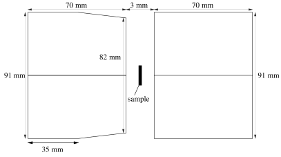
Figure 1: Schematic view of a possible $\gamma$-detection system consisting of two Clover-type detectors in close geometry RDH12 .

The disadvantage is that the neutron energies are not known anymore at the time of the activity measurement. Only spectrum-averaged cross sections ($SACS$) can be determined, therefore it is called integral measurement:

$$SACS=\frac{\int{\sigma(E)\Phi(E)\mathrm{d}E}}{\int{\Phi(E)\mathrm{d}E}}$$ (10)

The number of atoms produced during the activation ($N_{\mathrm{activation}}$) can be written as:

$$N_{\mathrm{activation}}=N_{\mathrm{sample}}\Phi_{\mathrm{n}}\sigma t_{\mathrm{a}}~{},$$ (11)

where $\Phi_{n}$ is the energy-integrated neutron flux (cm^-2s^-1). If the activation time ($t_{\mathrm{a}}$) is short compared to the half-life time ($t_{1/2}$) of the radioactive neutron-capture product, the freshly produced activity ($A_{\mathrm{activation}}$) increases linearly with the activation time:

$$A_{\mathrm{activation}}\approx\lambda N_{\mathrm{activation}}=\frac{\ln{2}}{t_{1/2}}N_{\mathrm{sample}}\Phi_{\mathrm{n}}\sigma t_{\mathrm{a}}$$ (12)

Small cross sections $\sigma$ or small samples $N_{\mathrm{sample}}$ can therefore partly be compensated with longer activation time or increased neutron flux. The amount of nuclei, which decays before the activity measurement can be accounted for, see section 2.2. Samples smaller than 1 $\upmu$g could be investigated with neutrons in the keV-regime with this very sensitive method. In some cases, the sample itself was already radioactive. This limited the amount of sample material to 28 ng of ¹⁴⁷Pm RAH03 and about 1 $\upmu$g of ⁶⁰Fe URS09 .

Even if no $\gamma$-rays are emitted, the method can be applied. The detection setup and sample preparation however are more demanding because very thin samples are required in order to detect the emitted particles. Examples are the successful detection of delayed emitted electrons after activation of ³⁴S using a silicon $\beta$-spectrometer RSK00 or of $\alpha$-particles following the ⁷Li(n,$\gamma$)⁸Li reaction using an ionization chamber HKW98 .

If the half-life of the product is very long, it might not be feasible to determine the activity of the capture product. In some of those cases, e.g. ⁶²Ni(n,$\gamma$) NPA05 , it is possible to count the number of produced atoms with accelerator mass spectroscopy. If, however, the half-life is very short, it might be necessary to repeatedly irradiate and count the decays BRW94 . This can be carried out as an automated cyclic activation as in the case of ¹⁴C(n,$\gamma$) RHF08 .

2.2 Correction for nuclei decayed during the activation

If the length of the activation can not be neglected compared to the half-life of the activation product, some of the freshly produced nuclei decay already during the irradiation phase. With

• $t=0$ .. the beginning of activity counting

• $N_{0}=N(t=0)$ .. number of produced nuclei at the beginning of activity counting

• $N(t)=N_{0}\exp{(-\lambda t)}$ .. no feeding, just radioactive decays

• $t_{\mathrm{m}}$ .. real time of activity counting

• $t_{\mathrm{w}}$ .. time between end of activation and beginning of activity counting

• $C_{\gamma}$ .. the number of counts in the line corresponding to the observed $\gamma$

• $\epsilon_{\gamma}$ .. the detection efficiency of the observed $\gamma$

• $I_{\gamma}$ .. the line intensity - number of emitted $\gamma$-rays per decay

the number of decays during activity measurement can be expressed as

$$\Delta N = N_{0}-N(t_{\mathrm{m}})$$ (13)

$$= N_{0}\left(1-\mbox{e}^{-\lambda t_{\mathrm{m}}}\right)$$ (14)

$$= \frac{C_{\gamma}}{\epsilon_{\gamma}I_{\gamma}}$$ (15)

hence:

$$N_{0}=\frac{C_{\gamma}}{\epsilon_{\gamma}I_{\gamma}}\frac{1}{1-\mbox{e}^{-\lambda t_{\mathrm{m}}}}$$ (16)

Therefore the number of nuclei at the end of activation is:

$$N(-t_{\mathrm{w}}) = N_{0}\mbox{e}^{\lambda t_{\mathrm{w}}}$$ (17)

$$= \frac{C_{\gamma}}{\epsilon_{\gamma}I_{\gamma}}\frac{1}{1-\mbox{e}^{-\lambda t_{\mathrm{m}}}}\frac{1}{\mbox{e}^{-\lambda t_{\mathrm{w}}}}$$ (18)

$N(-t_{w})$ is the number of produced nuclei reduced by the decays that occurred already during the activation. The number of atoms present during the activation follows as:

$$\dot{N}(t)=P(t)-\lambda N(t)$$ (19)

Assuming a constant production rate $P(t)=P$, and $N(t_{\mathrm{start}})=0$, the solution is:

$$N(t)=\frac{P}{\lambda}\left(1-\mbox{e}^{-\lambda(t-t_{\mathrm{start}})}\right)$$ (20)

Hence the number of nuclei at the end of the activation ($t_{\mathrm{end}}=-t_{\mathrm{w}};t_{\mathrm{a}}=t_{\mathrm{end}}-t_{\mathrm{start}}$):

$$N(t_{\mathrm{end}}) = \frac{P}{\lambda}\left(1-\mbox{e}^{-\lambda(t_{\mathrm{end}}-t_{\mathrm{start}})}\right)$$ (21)

$$= \frac{P}{\lambda}\left(1-\mbox{e}^{-\lambda t_{\mathrm{a}}}\right)$$ (22)

However, the number of produced nuclei is:

$$N_{\mathrm{activation}}=\int_{t_{\mathrm{start}}}^{t_{\mathrm{end}}}P\mbox{d}t=Pt_{\mathrm{a}}$$ (23)

It therefore follows for the $f_{\mathrm{b}}$-factor:

$$f_{\mathrm{b}}:=\frac{N(t_{\mathrm{end}})}{N_{\mathrm{activation}}}=\frac{1-\mbox{e}^{-\lambda t_{\mathrm{a}}}}{\lambda t_{\mathrm{a}}}$$ (24)

With the equations above, one finds for the number of produced nuclei:

$$N_{\mathrm{activation}} = N(-t_{\mathrm{w}})/f_{\mathrm{b}}$$ (25)

$$= \frac{C_{\gamma}}{\epsilon_{\gamma}I_{\gamma}}\frac{1}{1-\mbox{e}^{-\lambda t_{\mathrm{m}}}}\frac{1}{\mbox{e}^{-\lambda t_{\mathrm{w}}}}\frac{1}{f_{\mathrm{b}}}$$ (26)

$$= \frac{C_{\gamma}}{\epsilon_{\gamma}I_{\gamma}}\frac{1}{1-\mbox{e}^{-\lambda t_{\mathrm{m}}}}\frac{1}{\mbox{e}^{-\lambda t_{\mathrm{w}}}}\frac{\lambda t_{\mathrm{a}}}{1-\mbox{e}^{-\lambda t_{\mathrm{a}}}}$$ (27)

If the production rate during the activation is not constant, because the irradiation is changing or the activation is interrupted, eq. (24) can easily be generalized. Under real experimental conditions, it is very often appropriate to assume a production rate, which is constant over some periods of time. This occurs either, because several activations are performed or the production rate (proportional to neutron flux or beam current) is constant over time intervals, which are small compared to the half life of the produced isotope. Under those assumptions, the activation can be treated as a sequence of several smaller activations with constant production rates $P_{i}$, activation times $t_{\mathrm{a},i}$, starting times $t_{\mathrm{start},i}$ and ending times $t_{\mathrm{end},i}$. The time between the end of each activation until the end of the last activation will be called $t_{\mathrm{w},i}$, while $t_{\mathrm{w}}$ is the time between the end of the last activation and the beginning of the activity counting. Then eq. (23) becomes:

$$N_{\mathrm{activation}} = \sum_{i}\int_{t_{\mathrm{start},i}}^{t_{\mathrm{end},i}}P_{i}\mbox{d}t$$ (28)

$$= \sum_{i}P_{i}t_{\mathrm{a},i}$$ (29)

and eq. (21) becomes:

$$N_{i}(t_{\mathrm{end},i}) = \frac{P_{i}}{\lambda}\left(1-\mbox{e}^{-\lambda t_{\mathrm{a},i}}\right)$$ (30)

Therefore the nuclei after the last activation are the sum of all left-overs of all activations:

$$N(t_{\mathrm{end}}) = \sum_{i}N_{i}(t_{\mathrm{end},i})\mbox{e}^{-\lambda t_{\mathrm{w},i}}$$ (31)

$$= \sum_{i}\frac{P_{i}}{\lambda}\left(1-\mbox{e}^{-\lambda t_{\mathrm{a},i}}\right)\mbox{e}^{-\lambda t_{\mathrm{w},i}}$$ (32)

and the $f_{\mathrm{b}}$-factor can be written as:

$$f_{\mathrm{b}}=\frac{N(t_{\mathrm{end}})}{N_{\mathrm{activation}}}=\frac{\sum_{i}P_{i}\left(1-\mbox{e}^{-\lambda t_{\mathrm{a},i}}\right)\mbox{e}^{-\lambda t_{\mathrm{w},i}}}{\lambda\sum_{i}P_{i}t_{\mathrm{a},i}}$$ (33)

It is interesting to look into some special cases of this equation. First, if the individual activation times are short compared to the half-life of the activation product, for instance if the neutron flux or beam current is recorded over short time intervals, eq. (33) becomes:

$$f_{\mathrm{b}}=\frac{\sum_{i}P_{i}t_{\mathrm{a},i}\mbox{e}^{-\lambda t_{\mathrm{w},i}}}{\sum_{i}P_{i}t_{\mathrm{a},i}}$$ (34)

Further, if the activation times are equal for all activations ($t_{\mathrm{a},i}==t_{\mathrm{a}}$), one finds:

$$f_{\mathrm{b}}=\frac{\sum_{i}P_{i}\mbox{e}^{-\lambda t_{\mathrm{w},i}}}{\sum_{i}P_{i}}$$ (35)

Let the production rate be:

$$P(t)=\sigma N_{\mathrm{sample}}\Phi(t)$$ (36)

then eq. (35) becomes:

$$f_{\mathrm{b}}=\frac{\sum_{i}\Phi_{i}\mbox{e}^{-\lambda t_{\mathrm{w},i}}}{\sum_{i}\Phi_{i}}$$ (37)

2.3 Partial cross sections to isomers and ground state

One additional advantage of activation measurements is the possibility to determine the partial cross sections populating isomeric states or the ground state of the reaction product.

If only one isomeric state is of importance and if it decays partly to the ground state, the neutron capture cross section feeding the isomeric state can be determined via the same $\gamma$-lines as for the captures to the ground state. The advantage of this method is that all uncertainties caused by detection efficiency, $\gamma$-ray and neutron self-absorption in the sample, cascade corrections, and line intensities are canceling out in a relative measurement of the cross sections. The only systematic uncertainties left are due to time correlated measurements. The time dependence of the isomeric state is a simple exponential behavior:

$$N^{\mathrm{m}}(t)=N^{\mathrm{m}}(0)=e^{-\lambda^{\mathrm{m}}t}$$ (38)

while the one of the ground state abundance is given by the differential equation:

$$\frac{dN^{\mathrm{g}}}{dt}(t)=-\lambda^{\mathrm{g}}\cdot N^{\mathrm{g}}(t)+f_{i}\cdot\lambda^{\mathrm{m}}\cdot N^{\mathrm{m}}(t),$$ (39)

where $\lambda$ is the decay constant and $f_{i}$ the part of internal decays feeding the ground state. The solution is:

$$N^{\mathrm{g}}(t)=N^{\mathrm{g}}(0)\cdot e^{-\lambda^{\mathrm{g}}t}+\frac{\lambda^{\mathrm{m}}}{\lambda^{\mathrm{g}}-\lambda^{\mathrm{m}}}f_{i}\cdot N^{\mathrm{m}}(0)\left(e^{-\lambda^{\mathrm{m}}t}-e^{-\lambda^{\mathrm{g}}t}\right)$$ (40)

The time dependence of the number of ground state nuclei and via $A(t)=\lambda N(t)$ the activity of the ground state decay is a sum of two exponential decays. If the half-life of the ground state is much shorter than the one of the isomeric state ($\lambda^{\mathrm{g}}\gg\lambda^{\mathrm{m}}$), the activity immediately after the activation is determined by the decay activity of the ground state

$$A^{\mathrm{g}}(t)=\lambda^{\mathrm{g}}\cdot N^{\mathrm{g}}(0)\cdot e^{-\lambda^{\mathrm{g}}t}$$ (41)

and the isomer decay determines the time dependence at much later times

$$A^{\mathrm{g}}(t)=\frac{\lambda^{\mathrm{g}}\lambda^{\mathrm{m}}}{\lambda^{\mathrm{g}}-\lambda^{\mathrm{m}}}f_{i}\cdot N^{\mathrm{m}}(0)\cdot e^{-\lambda^{\mathrm{m}}t}~{}.$$ (42)

An example of such an analysis is the activation of natural Te. Four isotopes with a total of 4 isomers and 3 ground state decays could be analyzed after the activation with keV-neutrons ReK02 .

2.4 Neutron spectra

The ⁷Li(p,n) reaction as a neutron source in combination with a Van de Graaff accelerator was used for almost thirty years at Forschungszentrum Karlsruhe. The development of new accelerator technologies CGK18 , in particular the development of radiofrequency quadrupoles (RFQ) has provided much higher proton currents than previously achievable. The additional development of liquid-lithium target technology to handle the target cooling opens a new era of activation experiments thanks to the enormously increased neutron flux. Projects like SARAF TPA15 and FRANZ WCD10 ; RCH09 , underline this statement.

While other neutron-energy distributions were used on occasion RSK00 ; RHF08 , the quasi-stellar neutron spectrum, which can be obtained by bombarding a thick metallic Li target with protons of 1912 keV slightly above the reaction threshold at 1881 keV, was the working horse at Karlsruhe BBK00 . Under such conditions, the ⁷Li(p,n)⁷Be reaction yields a continuous energy distribution with a high-energy cutoff at $E_{\mathrm{n}}$ = 106 keV. The produced neutrons are emitted in a forward cone of 120^∘ opening angle. The angle-integrated spectrum closely resembles a spectrum necessary to measure the Maxwellian averaged cross section at $kT$ = 25 keV RaK88 ; BeK80 (Fig. 2) i.e.,

$$\frac{dN}{dE}\propto E\cdot e^{-\frac{E}{kT}}\propto\sqrt{E}\cdot\phi_{{\mathrm{MB}}},$$ (43)

where $\phi_{{\mathrm{MB}}}$ is the Maxwellian distribution for a thermal energy of $kT$ = 25 keV, see eq. (3).

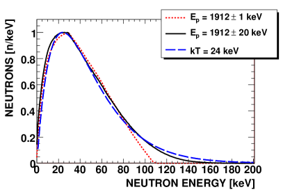
Figure 2: Comparison of the number of angle-integrated neutrons per linear energy bin for simulations using PINO that contain weighting and include a Gaussian proton-energy profile RHK09 . A sample of 10 mm radius and a Li-spot of 3 mm radius was assumed. All simulated spectra are normalized to a common maximum of 1.

The samples are typically sandwiched between gold foils and placed directly on the backing of the lithium target. A typical setup is sketched in Fig. 3. The simultaneous activation of the gold foils provides a convenient tool for measuring the neutron flux, since both the stellar neutron capture cross section of ¹⁹⁷Au RaK88 and the parameters of the ¹⁹⁸Au decay Aub83 are accurately known, see also section 4.

Figure 3: Typical activation setup. Neutrons are produced via the ⁷Li(p,n) reaction just above the production threshold. The emitted neutrons are then kinematically focussed into a cone with an opening angle of 120^∘. The sample is usually sandwiched by two gold foils in order to determine the neutron flux just before and behind the sample.

While the neutron spectrum for the standard case is very well understood, a tool for extrapolation to different experimental conditions is desired. Such changes of the standard setup typically include differences in the angle coverage of the sample, a different thickness of the lithium layer, or different proton energies. The extrapolation is, while conceptually obvious, not straight forward. After impinging onto the lithium layer, the protons are slowed down until they either leave the lithium layer (in case of a very thin layer) or fall below the (p,n) reaction threshold and do not contribute to the neutron production anymore. The double-differential (p,n) cross section changes significantly during this process, especially in the energy regime close to the production threshold. Additionally the kinematics of the reaction is important during the process. Since the Q-value of the reaction is positive, the reaction products, and the neutrons in particular, are emitted into a cone in the direction of the protons (Fig. 3). This effect becomes less and less pronounced as the proton energy increases. If the proton energy in the center-of-mass system is above 2.37 MeV, a second reaction channel ⁷Li(p,n)⁷Be^⋆ opens, which leads to a second neutron group at lower energies. To model these processes quantitatively, a tool to simulate the neutron spectrum resulting from the ⁷Li(p,n) reaction with a Monte-Carlo approach is indispensable. Therefore the highly specialized program PINO - Protons In Neutrons Out - was developed RHK09 . The power of this approach was demonstrated during an activation of ¹⁴C with different settings and correspondingly different average neutron energies between 25 keV and almost 1 MeV RHF08 .

While a temperature of $kT=25$ keV is very well suited for many nucleosynthesis simulations, other temperatures are of interest too. Since extrapolations from activations at a given energy become increasingly uncertain if the temperature is very different, activations with spectra corresponding to other energies are desirable. One approach is the superposition of different spectra. Fig. 4 and Table 1 show the results of a PINO-based study to emulate a spectrum corresponding to $kT=90$ keV. The final spectrum is a linear combination of five components.

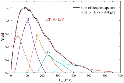
Figure 4: Superposition of different neutron spectra to approximate a spectrum corresponding to $kT=90~{}$keV. The neutron spectra were simulated using the online tool PINO RHK09 . The corresponding beam parameters are summarized in Table 1.

Table 1: Beam parameter used for the spectra in Fig. 4. The thickness of the lithium target was always 8 $\upmu$m, which corresponds to a proton-energy loss of 2 keV. The beam spot had a radius of 3 mm. The sample was a disc with a radius of 10 mm and negligible thickness.

spectrum	$E_{\textrm{p}}$	distance	scaling factor
ID	[keV]	[mm]
I	1936	6	0.563
II	1993	5	0.783
III	2093	3	0.535
IV	2145	4	0.273
V	2257	4	0.138

A very important ingredient is the double-differential ⁷Li(p,n) cross section in particular close to the reaction threshold. The current version of PINO contains data from Liskien and Paulson LiP75 above a proton energy of $E_{p}=1950$ keV and below an energy dependence as described by Lee and Zhou LeZ99 :

$$\sigma(E_{\mathrm{p}})=\frac{A}{E_{\mathrm{p}}}\frac{x}{(1+x)^{2}}$$ (44)

with

$$x=c_{0}\sqrt{1-\frac{E_{\mathrm{threshold}}}{E_{\mathrm{p}}}}$$ (45)

and

$$c_{0} = 6$$

$$A = 164.913$$

$$E_{\mathrm{threshold}} = 1.8804~{}\mathrm{MeV}.$$

Measurements of the ⁷Li(p,n) cross section very close to the threshold are difficult. An alternative method is the use of the reverse reaction, ⁷Be(n,p) BAM18 .

2.5 Impact of backing material

The neutrons produced in the ⁷Li(p,n) reactions have to pass a backing supporting the thin layer of lithium before they reach the sample. Depending on the backing material and thickness, this can not only reduce the number of neutrons but also alter the spectrum. A plain, neutron-energy-independent reduction would not alter the results of an activation measurement as described so far, since it would affect the sample in the same way as the neutron monitors. However, absolute measurements can be affected, see discussion in section 4.

The shape of the neutron spectrum is usually only slightly affected by the backing. Only under the very rare circumstances that the resonances in the sample are at the same energy as the flux reductions caused by the backing, the effect on the sample is different than the effect on the neutron monitor. This was the unfortunate case of an activation of a Cu sample behind a Cu backing (Figs. 5-7) HKU08 ; WBC17 .

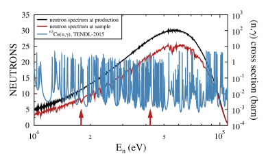
Figure 5: A 1 mm thick copper backing as commonly used during activation measurements has little effects on the neutron spectrum seen by the sample. However, in the case of a ⁶³Cu sample, flux reductions are at the same energy as the resonances in the sample (see arrows for clear examples). In total $10^{11}$ neutrons were simulated.

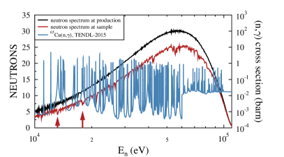
Figure 6: A 1 mm thick copper backing as commonly used during activation measurements has little effects on the neutron spectrum seen by the sample. However, in the case of a ⁶⁵Cu sample, flux reductions are at the same energy as the resonances in the sample(see arrows for clear examples). In total $10^{11}$ neutrons were simulated.

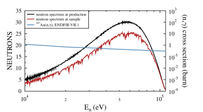
Figure 7: A 1 mm thick copper backing as commonly used during activation measurements has little effects on the neutron spectrum seen by the sample. Almost no effect is expected for a ¹⁹⁷Au sample. In total $10^{11}$ neutrons were simulated.

New and ongoing investigations based on Monte-Carlo simulations suggest that this effect can be neglected for almost all activations carried out by the Van de Graaff group at Karlsruhe. The only exceptions found so far are ^63,65Cu HKU08 and ⁶²Ni NPA05 .

3 Differential cross section measurements

3.1 General idea

Neutron-induced cross sections usually show a strong resonant structure, caused by the existence of excited levels in the compound nucleus. The excitation function for a reaction can accordingly be divided into three regions, the resonance region, where the experimental setup allows to identify individual resonances, the unresolved resonance region, where the average level spacing is still larger than the natural resonance widths, and the continuum region, where resonances start to overlap. The border between the first two regions is determined by the average level spacing and by the neutron-energy resolution of the experiment.

The time-of-flight (TOF) method enables cross section measurements as a function of neutron energy. Neutrons are produced quasi-simultaneously by a pulsed particle beam, thus allowing one to determine the neutron flight time $t$ from the production target to the sample where the reaction takes place. For a flight path $L$, the neutron energy is

$$E_{{\mathrm{n}}}=m_{\mathrm{n}}c^{2}(\gamma-1)$$ (46)

where $m_{\mathrm{n}}$ is the neutron mass and $c$ the speed of light. The relativistic correction $\gamma=\left(\sqrt{1-(L/t)^{2}/c^{2}}\right)^{-1}$ can usually be neglected in the neutron energy range of interest in nucleosynthesis studies and Eq. 46 reduces to

$$E_{{\mathrm{n}}}=\frac{1}{2}m_{\mathrm{n}}\left(\frac{L}{t}\right)^{2}.$$ (47)

The TOF method requires that the neutrons are produced at well defined times. This is achieved by irradiation of an appropriate neutron production target with a fast-pulsed beam from particle accelerators. The TOF spectrum measured at a certain distance from the target is sketched in Fig. 8. The essential features are a sharp peak at $t=L/c$, the so-called $\gamma$-flash due to prompt photons produced by the impact of a particle pulse on the target, followed by a broad distribution of events when the neutrons arrive at the sample position, corresponding to the initial neutron energy spectrum.

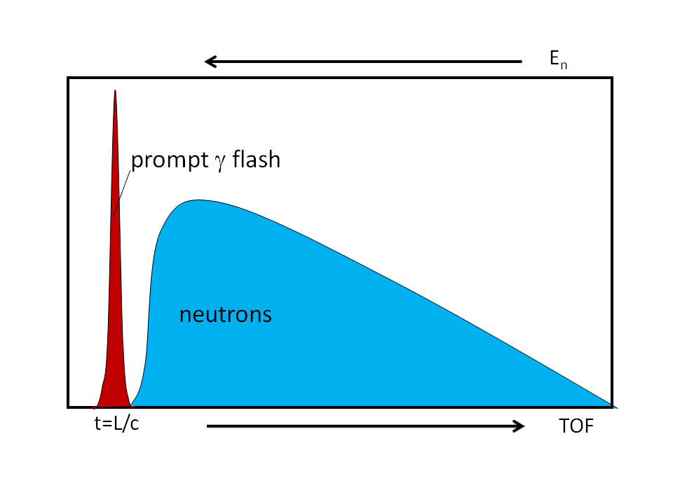
Figure 8: Schematic time-of-flight spectrum. The sharp peak at $t=L/c$ is caused by prompt photons produced by the impact of a particle pulse on the target. Neutrons reach the measurement station at later times and give rise to a broad distribution depending on their initial energies.

Neutron TOF facilities are mainly characterized by two features, the energy resolution $\Delta E_{\mathrm{n}}$ and the flux $\phi$. The neutron energy resolution is determined by the uncertainties of the flight path $L$ and of the neutron flight time $t$:

$$\frac{\Delta E_{\mathrm{n}}}{E_{\mathrm{n}}}=2\sqrt{\frac{\Delta t^{2}}{t^{2}}+\frac{\Delta L^{2}}{L^{2}}}$$ (48)

The neutron energy resolution can be improved by increasing the flight path, but only at the expense of the neutron flux, which scales with $1/L^{2}$. The ideal combination of energy resolution and neutron flux is, therefore, always an appropriate compromise. The energy resolution is affected by the Doppler broadening due to the thermal motion of the nuclei in the sample, by the pulse width of the particle beam used for neutron production, by the uncertainty of the flight path including the size of the production target, and by the energy resolution of the detector system.

3.2 Detection of the neutron-induced reaction

In TOF measurements, capture cross sections are determined via the prompt $\gamma$-ray cascade emitted in the decay of the compound nucleus. Total absorption calorimeters or total energy detection systems are the most common detection principles for measuring neutron capture cross sections.

The total energy technique is based on a device with a $\gamma$-ray detection efficiency, ($\varepsilon_{\gamma}$) proportional to $\gamma$ energy ($E_{\gamma}$):

$$\varepsilon_{\gamma}=kE_{\gamma}$$ (49)

Provided that the overall efficiency is low and that no more than one $\gamma$ is detected per event, the efficiency for detecting a capture event becomes independent of cascade multiplicity and de-excitation pattern, but depends only on the excitation energy of the compound nucleus, which is equal to the sum of neutron separation energy and kinetic energy in the center of mass before the formation of the compound nucleus. It can be shown that with the given assumptions the probability $\epsilon_{\mathrm{casc}}$ to detect any $\gamma$-ray out of a cascade of $n$ $\gamma$-rays can be written as:

$$\varepsilon_{\mathrm{casc}}=\sum_{i=1}^{n}\varepsilon_{\gamma}^{i}=\sum_{i=1}^{n}kE_{\gamma}^{i}=k\sum_{i=1}^{n}E_{\gamma}^{i}=k(Q+E_{CM})$$ (50)

A detector with an intrinsic proportionality of $E_{\gamma}$ and $\varepsilon_{\gamma}$ was first developed by Moxon and Rae MoR63 by combining a $\gamma$-to-electron converter with a thin plastic scintillator. Because of this conversion, Moxon-Rae detectors are essentially insensitive to low-energy $\gamma$ rays and were, therefore, used in TOF measurements on radioactive samples WiK78 ; WiK79a . The efficiency of Moxon-Rae detectors for capture events is typically less than a few percent.

Higher efficiencies of about 20% can be obtained by an extension of the Moxon-Rae principle originally proposed by Maier-Leibnitz Rau63 ; MaG67b . In these total energy detection systems the proportionality $E_{\gamma}$ - $\varepsilon_{\gamma}$ is extrinsically realized by an $a~{}posteriori$ treatment of the recorded pulse-height. This Pulse Height Weighting technique is commonly used with liquid scintillation detectors about one liter in volume, small enough for the condition to detect only one $\gamma$ per cascade. Present applications at neutron facilities n_TOF (CERN, Switzerland) and at GELINA (IRMM, Belgium) are using deuterated benzene (C₆D₆) as scintillator because of its low sensitivity to scattered neutrons. Initially, the background due to scattered neutrons had been underestimated, resulting in overestimated cross sections, particularly in cases with large scattering-to-capture ratios as pointed out by Koehler et al. KWG00 and Guber et al. GLS05 . With an optimized design, an extremely low neutron sensitivity of $\varepsilon_{\mathrm{n}}/\varepsilon_{\gamma}\approx 3\times 10^{-5}$ has been obtained at n_TOF PHK03 , which is especially important for light and intermediate-mass nuclei, where elastic scattering usually dominates the capture channel.

A total absorption calorimeter consists of a set of detectors arranged in 4$\pi$ geometry, thus covering the maximum solid angle. Because the efficiency for a single $\gamma$-ray of the capture cascade is usually close to 100% in such arrays, capture events are characterized by signals corresponding essentially to the Q-value of the reaction. Provided good resolution in $\gamma$ energy, gating on the Q-value represents, therefore, a possibility of significant background suppression.

Total absorption calorimeters exist at several TOF facilities. Most are using BaF₂ as scintillator material, which combines excellent timing properties, fairly good energy resolution, and low sensitivity to neutrons scattered in the sample. In fact, neutron scattering dominates the background in calorimeter-type detectors, because the keV-cross sections for scattering are typically 10 to 100 times larger than for neutron capture. In measurements at moderated neutron sources this background is usually reduced by an absorber surrounding the sample. Such a detector has been realized first at the Karlsruhe Van de Graaff accelerator WGK90a . This design, which consists of 42 crystals, is also used at the n_TOF facility at CERN GAA09 , while a geometry with 160 crystals has been adopted for the DANCE detector at Los Alamos HRF01 ; RBA04 . There are also $4\pi$ arrays made of NaI crystals MAA85 ; BDS94 , but in the astrophysically important keV region these detectors are suffering from the background induced by scattered neutrons, which are easily captured in the iodine of the scintillator.

3.3 White spectra

At white neutron sources, the highest neutron energy for which the neutron capture cross section can be determined is limited by the recovery time of the detectors after the $\gamma$ flash. While the accessible neutron energy range is practically not restricted for C₆D₆ detectors, BaF₂ arrays are more sensitive, depending on the respective neutron source. At n_TOF, for example, the BaF₂ calorimeter has been used only up to few keV so far GCM12 , whereas there are no strong limitations at DANCE at Los Alamos ERB08 . Recent tests suggest however that the NAUTILUS detector, which is strongly optimized for the handling of the $\gamma$-flash WGR18 ; RDF18 , can be used at n_TOF up to about 1 MeV, see Fig. 9.

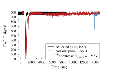
Figure 9: Output signal of a photomultiplier coupled to a BaF₂ crystal. The unit was positioned close to the beam line of experimental area 1 (EAR-1) at n_TOF about 200 m away from the spallation source GTB13 .The $\gamma$-flash occurs about 600 ns after the proton pulse hits the lead target producing the neutrons via spallation reactions. The flash-ADC-based data acquisition is saturated during the flash. However, neutrons with an energy of 1 MeV would arrive about 14 $\upmu$s after that. The detector would be able to accept events at that time, as shown by an exemplary waveform taken with a ⁸⁸Y calibration source. Dedicated nTOF pulsed are typically larger and cleaner than parasitic pulses, which are provided much more irregularly.

Independent of the detection system, measurements at higher neutron energies are increasingly difficult because the (n,$\gamma$) cross section decreases with neutron energy, while at the same time competing reaction channels, e.g. inelastic neutron scattering, are becoming stronger. Nevertheless, present techniques are covering the entire energy range of astrophysical relevance up to about 500 keV with sufficient accuracy.

3.4 Tailored spectra

In specific neutron spectra, e.g. in measurements with the Karlsruhe array, where the maximum neutron energy was about 200 keV, scattered neutrons can be partially discriminated via TOF between sample and scintillators because the capture $\gamma$ rays reach the detector before the scattered neutrons WGK90a . The idea is that neutrons scattered on the sample reach the detector later than the prompt $\gamma$-rays following the neutron capture events. This idea is particularly powerful if the flight path is short. While most of the experiments (see chapter 5) with the Karlsruhe array were performed with a flight path of 80 cm, even shorter flight paths are necessary to measure (n,$\gamma$) reactions on radioactive samples.

The present layout of the FRANZ facility at the Goethe University Frankfurt barely provides the high neutron fluxes needed to perform measurements on radioactive isotopes with comparably hard $\gamma$-ray emission like ⁸⁵Kr RCH09 ; CoR07 . Since the neutron production is already at the limits of the current technology, one option is to get closer to the neutron production target to increase the solid angle covered by the sample material. Such a TOF measurement can be performed with sufficient accuracy even with a flight path as short as a few centimeters (Fig. 10, left) RDF18 .

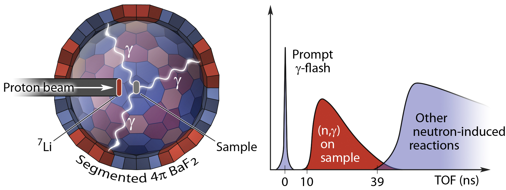
Figure 10: Left: Schematic setup of the planned neutron capture experiment with an ultra-short flight path of only 4 cm. Right: Anticipated time-of-flight spectrum RHH04 ; RDF18 .

In this case, the only feasible solution is to produce the neutrons inside a spherical $\gamma$-detector and distinguish between background from interactions with the detector material and the signal from neutron captures on the sample based on the time after neutron production as illustrated in Fig. 10, right. First, an initial $\gamma$-flash, occurring when the protons hit the neutron production target, is detected. Then the prompt $\gamma$-rays produced in the (n,$\gamma$) reaction at the sample induce a signal in the detector. Later, the neutrons from other reactions, such as scattering in the detector material, arrive in the detector with sufficient delay as they are traveling at much slower speed than the $\gamma$-rays, and produce background.

A detailed investigation of the geometry of the setup at an ultra-short flight path has been performed WGR18 within the framework of the NAUTILUS project. In contrast to the calorimeters used in such TOF experiments so far RLK14 ; RBA04 ; WGK90a , the calorimeter shell has to be much thinner in order to allow the neutrons to escape quickly enough. The geometry is based on the DANCE array RBA04 ; HRF01 , which was designed as a high efficiency, highly segmented 4$\pi$ BaF₂ array. The NAUTILUS array consists of up to 162 crystals of 4 different shapes, each covering the same solid angle. The high segmentation distributes the envisaged high count rate over many channels, leading to a significant increase of the maximal tolerable total count rate that can be processed by the DAQ. The NAUTILUS array has an inner radius of 20 cm and a thickness of 12 cm.

The advantage of this setup is the greatly enhanced neutron flux. Because of the reduction of the flight path from 1 m to 4 cm, the neutron flux will be increased by almost 3 orders of magnitude. The reduced time-of-flight resolution resulting in a reduced neutron-energy resolution is still sufficient for astrophysical and applied purposes. A comparison to the DANCE setup shows that, despite the much shorter flight path (4 cm vs. 20 m), a much better time resolution (1 ns vs. 125 ns) will be achieved at the proposed setup. Because of the different time structure of the proton beam at the FRANZ facility the energy resolution will almost be the same for both setups.

4 ¹⁹⁷Au(n,$\gamma$) - a cross section standard

Standard cross sections are important quantities in neutron experiments, because they allow to circumvent difficult absolute flux determinations by measuring simply cross section ratios. Therefore, a set of standard cross sections has been established and is periodically updated with improved data characterized by higher accuracies and/or wider energy ranges. A review of the most recent activity on neutron cross section standards can be found in CPH17 .

Considered as an official standard only at thermal neutron energy (25.3 meV) and between 200 keV and 2.5 MeV BZC07 ; CPS09 , the (n,$\gamma$) cross section of gold is commonly also used in the keV region as a reference for neutron capture measurements related to nuclear astrophysics as well as for neutron flux determinations in reactor and dosimetry applications.

From the experimental point of view ¹⁹⁷Au exhibits most favorable features. Mechanically it is a monoisotopic metal available in very high purity that can easily be shaped to any desired sample geometry. Its nuclear properties are equally interesting: A strong resonance at 4.9 eV allows for the determination of the neutron flux or for the normalization of capture yields in TOF measurements by means of the ”saturated resonance technique” SBD12 . The (n,$\gamma$) cross section in the keV region is rather large, thus facilitating the measurement of cross section ratios. And it is also easily applicable for neutron activation studies due to the decay of ¹⁹⁸Au with the emission of an intense 412 keV $\gamma$-ray line. Both the decay rate ($\lambda=0.25718(7)$ d^-1) and the intensity per decay ($I_{\gamma}=95.58(12)$%) Chu02 are accurately known and perfectly suited for practical applications.

4.1 Measurements

In 1988, a direct measurement of the ¹⁹⁷Au(n,$\gamma$) cross section based on the ⁷Li(p,n)⁷Be reaction, which used the ⁷Be activity for an absolute determination of the neutron exposure, i.e. without reference to another standard, claimed a very low systematic uncertainty of 1.5% RaK88 . This result, which referred to the average cross section over a quasi-Maxwellian neutron spectrum for a thermal energy of $kT=25$ keV, was found in very good agreement with the value calculated on the basis of the energy-dependent cross section Mac81 , but was systematically lower by 5 to 7% than the evaluated ¹⁹⁷Au(n,$\gamma$) cross section based on a variety of data sets, including other reaction channels.

To clarify this issue, the energy-dependent cross section has been measured at n_TOF and GELINA in an effort to provide accurate new data in the resolved resonance region MDV10 , and at keV neutron energies LCD11 ; MBD14 . Both measurements were performed with C₆D₆ detectors, but used different neutron flux standards, a combination of the ⁶Li(n,t) and ²³⁵U(n,f) reactions at n_TOF and the ¹⁰B(n,$\alpha$) cross section at GELINA. In each case, the capture yield was self-normalized to the saturated gold resonance at 4.9 eV. The combination of improved detection systems with detailed simulations and analysis techniques has yielded data sets with $MACS$ uncertainties slightly above 3% at n_TOF and between 1 and 2% at GELINA. The new results agree with each other within systematic uncertainties and confirm the difference of about 5% relative to the activation result of Ref. RaK88 .

In parallel to the TOF results from n_TOF and GELINA, also the quasi-stellar neutron spectrum at a thermal energy $kT=25$ keV were remeasured at the 7-MV Van de Graaff laboratory at JRC Geel FFK12 and using the PIAF facility at the 3.75 MV Van de Graaff accelerator of PTB Braunschweig LKM12 . Both measurements confirmed the neutron field reported previously RaK88 and showed that substantial effects related to slight shifts in the proton energy or to the spectral broadening of the proton beam could be excluded as the cause of the difference to the new TOF data. Instead, an activation performed in addition to the spectrum measurements at JRC-Geel FFK12 found a 5% higher cross section than Ref. RaK88 .

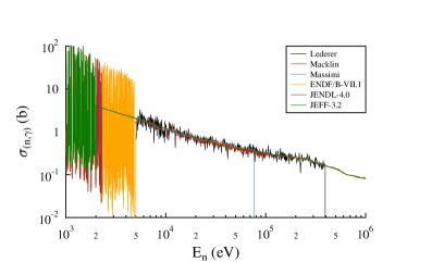
Figure 11: The main TOF data in the keV-neutron-energy regime compared with the evaluated data sets in the ENDF/B-VII.1 CHO11 , JEFF-3.2 JEFF30 ; JEFF31 , and JENDL-4.0 KSO11 libraries.

4.2 Monte Carlo simulations

The analyses of the new measurements all benefit from detailed Monte Carlo simulations of the involved corrections, whereas the earlier activation had tried to find an experimental access to these corrections. Therefore, Monte Carlo (MC) simulations of the experimental situation in Ref. RaK88 were performed in an attempt to localize the reason for the above discrepancy. For easier comparison of TOF and activation results all data sets were averaged over the quasi-Maxwellian spectrum centered at 25 keV used in RaK88 . In the following these spectrum-averaged cross sections are denoted as $SACS$.

The simulations were carried out by considering two volumes - the thin gold foil shaped as a section of a sphere and the backing of the ⁷Li target, which the neutrons have to pass in order to reach the gold foil, see Fig. 12. The neutrons were tracked according to the elastic scattering and capture cross sections adopted from the data libraries ENDF/B-VII.1, JEFF-3.2, and JENDL-4.0. In each case the Cu and Au cross sections were consistently taken from the same library. The neutrons were scattered isotropically, but the energy loss during elastic scattering was taken into account. Different backing thicknesses were simulated for direct comparison with the original activation data as given in Table III of Ref. RaK88 .

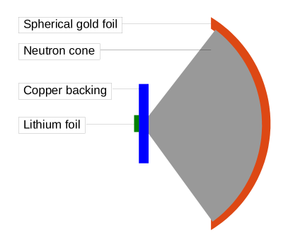
Figure 12: A spherical gold foil covering the entire neutron cone was activated during the ¹⁹⁷Au(n,$\gamma$) measurement by Ratynski & Käppeler RaK88 . Different backing materials and thicknesses were used. Only the backing and the gold foil were included in the simulations. The real setup was similar to the one in Fig. 3 except for the spherical sample.

Some components of the experimental uncertainties for different backing thickness provided in Ref. RaK88 are correlated. The same detector and line intensities were used for all activations. In order to better observe the trend when varying the backing thickness, it is better to compare the ratios of the different setups to a given setup, e.g. to the lithium target with the 1-mm Cu backing. Then all correlated variables cancel out and their uncertainty does not contribute.

Table 2 shows the results of this endeavor. The experimental data and the MC-based predictions with the evaluated cross sections of the data libraries are now in agreement within the experimental uncertainties - at least for the Cu-backing. It is not clear, whether the results for the Ag-backing disagree at this magnitude due to a problem with the Ag cross sections, because there is even a large scatter quoted in Ref. RaK88 . The simulations are offering a plausible explanation for the difference between the activation of RaK88 and the newest TOF measurements LCD11 ; MBD14 , namely that the effect of the backing was not properly taken into account during the activations. However, the simulation are not sufficiently consistent with the data for a reliable posterior correction. Nevertheless, they demonstrate that the new TOF measurements provide a reliable basis for establishing the (n,$\gamma$) cross section of ¹⁹⁷Au with an uncertainty of 1%, sufficient for re-considering gold as a neutron capture standard in the keV region.

Table 2: Ratio of Monte Carlo simulations of $SACS$ (mb) for $E_{\mathrm{proton}}=1912$ keV, each relative to the case of a 1-mm Cu-backing. These are compared to the experimental results obtained with different backing materials and thicknesses by Ratynski and Käppeler RHK09 ; RaK88 . Only uncorrelated uncertainties were considered for the experimental data. See Fig. 11 for the differential cross sections.

Backing	Ratio to 1 mm Cu backing
	ENDF	JEFF	JENDL	Ratynski
1.0 mm Cu	1	1	1	1
0.7 mm Cu	1.016	1.016	1.025	1.028 $\pm$ 0.012
0.5 mm Cu	1.032	1.029	1.031	1.042 $\pm$ 0.012
0.2 mm Ag	1.057	1.051	1.062	1.003-1.037
no backing	1.067	1.064	1.071

4.3 Evaluated cross section in data libraries

The evaluated cross sections in the data libraries ENDF/B-VII.1 CHO11 , JEFF-3.2 JEFF30 ; JEFF31 , and JENDL-4.0 KSO11 (which are considered as representative of similar compilations) are essentially based on the main TOF-measurements as illustrated in Fig. 11 and are, therefore, not affected by the discrepancy with the activation result of Ref. RaK88 . The experimental data are best represented by the ENDF/B-VII.1 evaluation, while the cross sections given in JEFF-3.2 and JENDL-4.0 are exceeding the ENDF/B-VII.1 data on average by about 3.5 and 2.4% between 10 and 100 keV, respectively.

4.4 Maxwellian average cross sections at stellar temperatures

The (n,$\gamma$) cross section of gold has been extensively used as a reference for numerous measurements devoted to studies of stellar nucleosynthesis in the slow neutron capture process (s process), which is associated with the He and C burning episodes of late evolutionary phases. The neutron spectrum typical of the various s-process sites discussed in nuclear astrophysics (see e.g. KGB11 ) is described by a Maxwell-Boltzmann distribution, because neutrons are quickly thermalized in the dense stellar plasma, and the effective stellar reaction cross sections are obtained by averaging the experimental data over that spectrum. The resulting Maxwellian averaged cross sections ($MACS$) are commonly compared for a thermal energy of $kT=30$ keV, but for realistic s-process scenarios a range of thermal energies has to be considered, from about 8 keV in the so-called ¹³C pocket, a thin layer in the He shell of thermally pulsing low mass AGB stars, to about 90 keV during carbon shell burning in massive stars.

To cover this full range, (n,$\gamma$) cross sections $\sigma(E)$ are needed at least in the energy window 1 keV and 1 MeV. Whenever experimental data are available only for part of this range, cross section calculations are required for filling the gaps. In this context, theoretical cross sections obtained via the Hauser-Feshbach approach are indispensable Rau14 .

With equation 6 the $MACS$ of ¹⁹⁷Au was calculated by separating the required neutron energy range into three regions:

$$MACS = \frac{2}{\sqrt{\pi}}\frac{1}{(kT)^{2}}\cdot\large(I_{\mathrm{low}}+I_{\mathrm{exp}}+I_{\mathrm{high}}\large)$$ (51)

$$I_{\mathrm{low}} = \int_{0}^{E_{\mathrm{low}}}\eta\cdot\sigma_{\mathrm{lib}}(E)\cdot E\cdot\exp{\left(-\frac{E}{kT}\right)}\mbox{d}E$$ (52)

$$I_{\mathrm{exp}} = \int_{E_{\mathrm{low}}}^{E_{\mathrm{high}}}\sigma_{\mathrm{exp}}(E)\cdot E\cdot\exp{\left(-\frac{E}{kT}\right)}\mbox{d}E$$ (53)

$$I_{\mathrm{high}} = \int_{E_{\mathrm{high}}}^{\infty}\eta\cdot\sigma_{\mathrm{lib}}(E)\cdot E\cdot\exp{\left(-\frac{E}{kT}\right)}\mbox{d}E$$ (54)

where $E_{\mathrm{low}}$ MBD14 and $E_{\mathrm{high}}$ define the range of the new experimental data LCD11 . At lower and higher energies the evaluated cross sections $\sigma_{lib}$ have been adopted from the current data libraries with an optional normalization factor

$$\eta=\frac{\int_{E_{\mathrm{low}}}^{E_{\mathrm{high}}}\sigma_{\mathrm{exp}}(E)\mbox{d}E}{\int_{E_{\mathrm{low}}}^{E_{\mathrm{high}}}\sigma_{\mathrm{lib}}(E)\mbox{d}E}$$ (55)

For the update of the ¹⁹⁷Au(n,$\gamma$) cross section we adopted $\eta=1$ and the following uncertainties for the data sets used:

• $\pm 5$% in region $I_{\mathrm{low}}$ ($E_{\mathrm{n}}\leq 3.5$ keV) (ENDF/B-VII.1 CHO11 )

• $\pm 1$% in region $I_{\mathrm{high}}$ ($E_{\mathrm{n}}\geq 400$ keV), where the cross section is an established standard (ENDF/B-VII.1 CHO11 ), and

• $\pm 1$% systematic uncertainty in region $I_{\mathrm{exp}}$ ($3.5$ keV $\leq E_{\mathrm{n}}\leq 400$ keV) together with the statistics quoted in Refs. LCD11 ; MBD14 .

In Table 3 the corresponding $MACS$ results for $kT=30$ keV are compared for the combination of three experimental data sets and three different libraries.

Table 3: $MACS$ (mb) for $kT=30$ keV. See Fig. 11 for the differential cross sections.

Data set	ENDF	JEFF	JENDL
Macklin Mac82a	586.2	588.3	587.1
Lederer LCD11	610.6	618.4	616.2
Massimi MBD14	610.5	614.6	610.6
ENDF/B-VII.1	616.5	***	***
JEFF-3.2	***	626.0	***
JENDL-4.0	***	***	634.0

The comparison shows remarkable agreement within 1% between the results based on the new TOF data LCD11 ; MBD14 and the ENDF/B-VII.1 evaluation, all very well compatible with the direct quotes of Lederer et al. LCD11 and Massimi et al. MBD14 of $611\pm 22$ mb and $613.3\pm 6$ mb, respectively. Somewhat larger differences are obtained with the evaluated cross sections from the other libraries. In view of this situation, an improved set of $MACS$ data for ¹⁹⁷Au has been determined by combining the new TOF results LCD11 ; MBD14 above 3.5 keV with the ENDF/B-VII.1 evaluation below that energy as summarized in Table 4.

Table 4: Improved $MACS$ values (mb) of ¹⁹⁷Au for the range of thermal energies of relevance for s-process nucleosynthesis.

$kT$ (keV)	$MACS_{\mathrm{197Au}}$ (mb)
5	2056 $\pm$ 37
10	1241 $\pm$ 14
15	940 $\pm$ 10
20	781 $\pm$ 8
25	681 $\pm$ 7
30	612 $\pm$ 6
40	521 $\pm$ 5
50	463 $\pm$ 5
60	423 $\pm$ 4
80	367 $\pm$ 4
100	329 $\pm$ 3

The excellent agreement of the new TOF data motivated the Standard Commission of the IAEA to consider a timely revision of the gold cross section and to envisage an extension of the gold standard into the keV region Cap18 .

We will discuss the impact of the new cross section on a number of TOF-measurements in the next section. The change of the differential neutron capture cross section of ¹⁹⁷Au has also implication for past and future activation experiments, which used or will use gold as a reference. Ratynski & Käppeler recommended $SACS=586$ mb for the spectrum described in Figs. 2 and 3 for a spherical sample covering the entire neutron cone. Based on the new cross section, we recommend:

$$SACS_{\mathrm{197Au,sphere}}=622.7\pm 6.2~{}\mathrm{mb}$$ (56)

For flat samples covering the entire neutron cone, which will be used in most experiments, we recommend

$$SACS_{\mathrm{197Au,flat}}=651.6\pm 6.5~{}\mathrm{mb}$$ (57)

The difference of 5% is a result of the fact that low-energy neutrons are on average emitted at larger angles and will therefore pass through more sample material than high-energy neutrons, compare Figs. 3 and 12. The cross section differential cross section at higher energies, however, is smaller.

5 Renormalization of TOF measurements

A consequence of the revised MACS-data of ¹⁹⁷Au is the re-evaluation of all cross sections obtained in previous TOF measurements, which were using the gold cross section recommended in RaK88 as a reference. This concerns, for example, the data listed in the compilation of the Karlsruhe Astrophysical Database of Nucleosynthesis in Stars (KADoNiS) DHK06 , which need to be corrected as they were consistently normalized to that work. In particular, this holds true for all TOF measurements carried out at the Karlsruhe Van-de-Graaff accelerator.

To this end, the $MACS$ are calculated according to Eq. (51), where $E_{low}$ and $E_{high}$ define the range of experimental data, $\sigma_{exp}$ denotes the experimental results- if possible directly the cross section ratio to ¹⁹⁷Au(n,$\gamma$), and $\eta$ is the respective normalization factor over the range of the experimental data, which falls in the range between 0.8 and 1.2. The experimental data are complemented with evaluated cross sections, $\sigma_{lib}$, which were taken from ENDFB-VII.1 except for a few cases.

The adopted procedure is using the following input:

• ¹⁹⁷Au

  • $I_{\mathrm{low}}$ - 5%, ENDF/B-VII.1, CHO11

  • $I_{\mathrm{high}}$ - 1%, ENDF/B-VII.1, CHO11

  • $I_{\mathrm{exp}}$ - 1% systematics, statistics as quoted LCD11 ; MBD14

• ^{170,171,172,173,174,176}Yb

  • $I_{\mathrm{low}}$ - 20%, JENDL-4.0 - KSO11

  • $I_{\mathrm{high}}$ - 10%, JENDL-4.0 - KSO11

  • $I_{\mathrm{exp}}$ - as quoted WVA00a

• ¹⁸⁰Ta

  • $I_{\mathrm{low}}$ - 20%, JEFF-3.2 JEFF30 ; JEFF31

  • $I_{\mathrm{high}}$ - 10%, JEFF-3.2 JEFF30 ; JEFF31

  • $I_{\mathrm{exp}}$ - as quoted WVA04

• All other isotopes

  • $I_{\mathrm{low}}$ - 20%, ENDF/B-VII.1, CHO11

  • $I_{\mathrm{high}}$ - 10%, ENDF/B-VII.1, CHO11

  • $I_{\mathrm{exp}}$ - as quoted

The essential features of the updated $MACS$ tables are illustrated at a few characteristic examples. The gold $MACS$ in Fig. 13 represents a case, which could be based on accurate energy-differential data in all three regions. Accordingly, the only difference to the previous KADoNiS versions is due to the 5% renormalization described in Sec. 4. The $MACS$ values for ¹⁷²Yb are typical for most cases derived from the accurate TOF data obtained with the Karlsruhe 4$\pi$ BaF₂ detector, which are spanning a neutron energy range from a few to about 220 keV. Accordingly, the larger uncertainties from the evaluated data adopted in the low and high energy regions are affecting the $MACS$ data at $kT\geq 70$ keV (Fig.15). Somewhat stronger effects in the low energy part are observed for isotopes with a pronounced resonance structure, e.g. for ¹⁴²Nd (Fig.14). An illustrative example is the case of ¹⁸⁰Ta (Fig 16). The extremely rare isotope was only available with an enrichment of 5.5% WVA01 ; WVA04 . The remainder of the sample was ¹⁸¹Ta. This resulted in a very limited range of experimental data. The lowest energy bin was 10-12.5 keV. In particular the $MACS$ at low temperatures is therefore basically not constrained by experimental data. The evaluations used by Wisshak $et~{}al.$ NKR92 ; RaT00 ; BeM82 to supplement the experimental data of ¹⁸⁰Ta(n,$\gamma$) had a different energy dependence than the currently used evaluation.

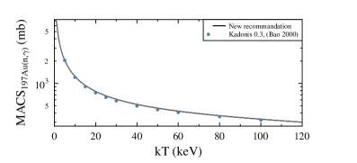
Figure 13: New (based on LCD11 ; MBD14 ; CHO11 )and old RaK88 ; BBK00 ; DHK06 recommendation for the $MACS$ of ¹⁹⁷Au.

Figure 14: New and old WVK98a ; WVK98b ; BBK00 ; DHK06 recommendation for the $MACS$ of ¹⁴²Nd.

Figure 15: New and old WVA00a ; BBK00 ; DHK06 recommendation for the $MACS$ of ¹⁷²Yb.

Figure 16: New and old WVA04 ; BBK00 ; DHK06 recommendation for the $MACS$ of ¹⁸⁰Ta.

In total 64 sets of MACS data have been updated and will be included in the next version of KADoNiS (1.0). The corresponding $MACS$ can be found in the appendix.

6 Indirect approaches

Direct measurements of neutron-induced cross sections are particularly difficult. Indirect methods are therefore often the only possibility to improve our knowledge. Well established indirect approaches are replacing the (n,$\gamma$) reaction with a surrogate reaction or measuring the time-reversed ($\gamma$,n) reaction. So far not done at all is the inverse kinematics approach, which is in fact also a direct measurement.

6.1 Surrogate

Surrogate reactions have been successfully used for obtaining neutron-induced fission cross sections EAB05 . This approach is using a charged particle reaction for producing the same compound system as in the neutron reaction of interest, Fig. 17. In this way, a short-lived target isotope can be replaced by a stable or longer-lived target. For neutron capture reactions, however, the method is challenged because the compound nucleus that is produced in the surrogate reaction is characterized by a spin-parity distribution that can be very different from the spin-parity distribution of the compound nucleus occurring in the direct (n,$\gamma$) reaction FDE07 ; EBD12 ; EBC17 .

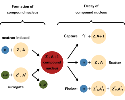
Figure 17: A neutron-induced reaction can be described as a multi-step process. The nucleus will first absorb the neutron forming a compound nucleus in an excited state. Afterwards it can either de-excite via $\gamma$-emission (capture), neutron emission (inelastic scattering) or split into two fragments (fission). The fission fragments in-turn are highly excited and will typically emit neutrons before they decay towards the valley of stability. In a surrogate reaction, the compound nucleus is produced by a different reaction.

6.2 Time-reversed

The Coulomb dissociation (CD) method can be used to determine the desired cross section of the reaction A(n,$\gamma$)B via the inverse reaction B($\gamma$,n)A by applying the detailed balance theorem, Fig. 18 BBR86 . It has been shown that this method can be successfully applied if the structure of the involved nuclei is not too complicated, as in the case of the reaction ¹⁴C(n,$\gamma$)¹⁵C RHF08 ; NFA09 . In case of heavier nuclei, this approach is usually less conclusive, since the CD cross section only constraints the direct decay to the ground state of the compound nucleus UAA14 . If the reaction product B is short-lived, the CD method can be applied at radioactive beam facilities HTW17 .

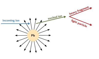
Figure 18: Schematic drawing of the Coulomb dissociation. If an ion traveling close to the speed of light passes close by a high-Z nucleus, it can get excited via interaction with the strong Coulomb field. If the excitation is higher than the binding energy of the constituents of the nucleus, they can be emitted, hence dissociated. The emitted particles are typically protons or neutrons, but sometimes also $\alpha$-particles.

Limitations of the CD method are (i) the applicability of this method to heavier nuclei close to the valley of stability due to the high level density in the compound nucleus, and (ii) because the resolution of current facilities of $\geq 100$ keV is not sufficient to constrain the astrophysically relevant cross section.

Restriction (i) is alleviated in r-process studies, because the level density is rapidly decreasing as the Q-values drops towards the neutron drip line. This implies that fewer levels are important, and the part of the capture cross section, which can be constrained via the inverse reaction, increases. Restriction (ii) motivated the development of improved experimental approaches such as NeuLAND@FAIR, which aims for an energy resolution of better than 50 keV BAA11 .

If the product is stable or very long-lived, also real photons can be used to study B($\gamma$, n)A reactions SMV03 ; Wel08 . In principle the same restrictions apply as for the Coulomb dissociation method.

6.3 Inverse kinematics

A completely different approach is to investigate neutron-induced reactions in inverse kinematics. This requires a beam of radioactive ions cycling in a storage ring with 100 $A$keV or less and a neutron target. Radioactive ions close to stability can be produced with high intensities using ISOL-techniques and storage rings for low beam energies, which require extremely high vacuum, are under construction, e.g. the CRYRING at GSI/FAIR HHS13 or the CSR at MPK/Heidelberg HBB11 . The neutron target could be either a reactor coupled with the storage ring to obtain an interaction zone near the core ReL14 or the moderator surrounding a spallation target RGH17 . Different materials with low neutron-absorbing cross sections like D₂O, Be or C are suited RBD18 . The scheme of such a setup is sketched in Fig. 19.

Figure 19: Neutrons are produced by protons impinging on a tungsten spallation target (brown). The proton beam pipe (red) is orientated perpendicular to the ion beam pipe (light brown). The beam pipes do not intersect. The neutrons produced in the spallation process are moderated in the surrounding moderator (blue). They penetrate the ion beam pipe and act as a neutron target for the ions. The ion beam pipe is part of a storage ring outside the moderator. The storage ring may contain additional equipment like an electron cooler (green), Schottky pickups and particle detectors (gray).

7 Conclusion

Most of the experiments determining neutron-induced cross sections in the astrophysically important energy regime between 1 keV and 1 MeV are either based on the activation or the time-of-flight method. Even after decades of application, both techniques have lots of potential for improvements. Very often nuclear data, which are used during the analysis of the experiments, will get improved later. This includes decay properties but also reference cross sections. A careful re-evaluation of published results is only possible, if all the necessary raw data are provided. The new evaluation of the ¹⁹⁷Au(n,$\gamma$) cross section implied the re-evaluation of 63 other isotopes with experimental information from TOF experiments. We recommend a new spectrum-averaged cross section for the widely used ⁷Li(p,n) activation setup with neutron energies around $kT\approx 25$ keV. This will affect many isotopes and will be published separately.

Appendix

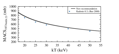
Figure 83: New (based on LCD11 ; MBD14 ; CHO11 ) and old RaK88 ; BBK00 ; DHK06 recommendation for the $MACS$ of ¹⁹⁷Au.

Figs. 20-83 show the results of the re-normalization for 64 isotopes separately.

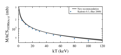
Figure 20: New and old WVK90 ; BBK00 ; DHK06 recommendation for the $MACS$ of ¹⁰³Rh.

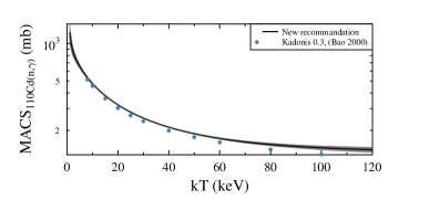
Figure 21: New and old WVK02 ; BBK00 ; DHK06 recommendation for the $MACS$ of ¹¹⁰Cd.

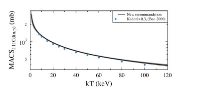
Figure 22: New and old WVK02 ; BBK00 ; DHK06 recommendation for the $MACS$ of ¹¹¹Cd.

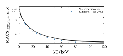
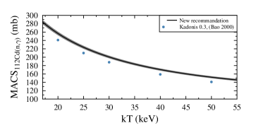
Figure 23: New and old WVK02 ; BBK00 ; DHK06 recommendation for the $MACS$ of ¹¹²Cd.

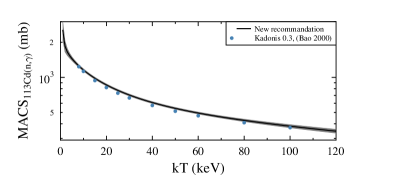
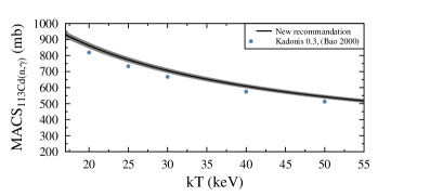
Figure 24: New and old WVK02 ; BBK00 ; DHK06 recommendation for the $MACS$ of ¹¹³Cd.

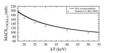
Figure 25: New and old WVK02 ; BBK00 ; DHK06 recommendation for the $MACS$ of ¹¹⁴Cd.

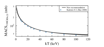
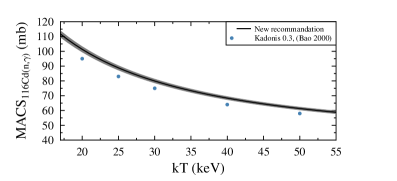
Figure 26: New and old WVK02 ; BBK00 ; DHK06 recommendation for the $MACS$ of ¹¹⁶Cd.

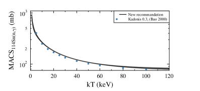
Figure 27: New and old WVT96a ; BBK00 ; DHK06 recommendation for the $MACS$ of ¹¹⁴Sn.

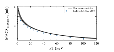
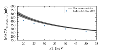
Figure 28: New and old WVT96a ; BBK00 ; DHK06 recommendation for the $MACS$ of ¹¹⁵Sn.

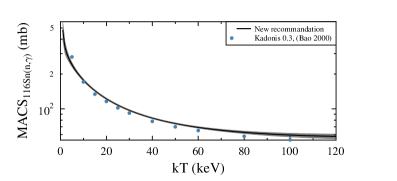
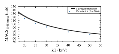
Figure 29: New and old WVT96a ; BBK00 ; DHK06 recommendation for the $MACS$ of ¹¹⁶Sn.

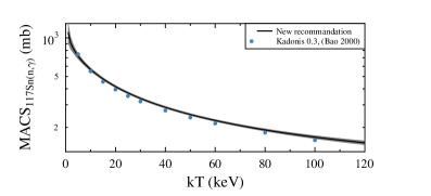
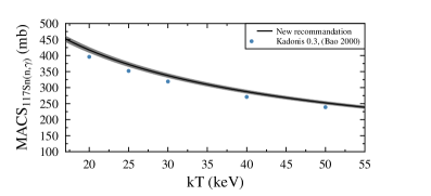
Figure 30: New and old WVT96a ; BBK00 ; DHK06 recommendation for the $MACS$ of ¹¹⁷Sn.

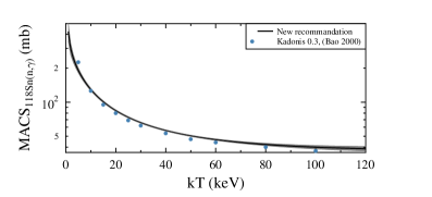
Figure 31: New and old WVT96a ; BBK00 ; DHK06 recommendation for the $MACS$ of ¹¹⁸Sn.

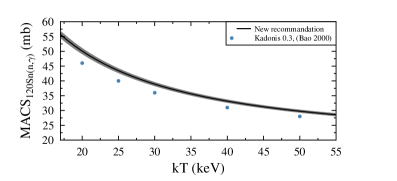
Figure 32: New and old WVT96a ; BBK00 ; DHK06 recommendation for the $MACS$ of ¹²⁰Sn.

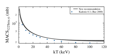
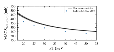
Figure 33: New and old WVK92 ; BBK00 ; DHK06 recommendation for the $MACS$ of ¹²²Te.

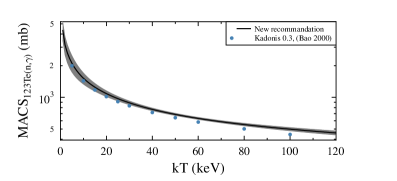
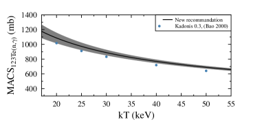
Figure 34: New and old WVK92 ; BBK00 ; DHK06 recommendation for the $MACS$ of ¹²³Te.

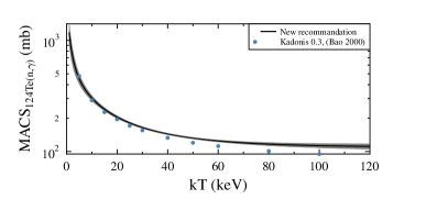
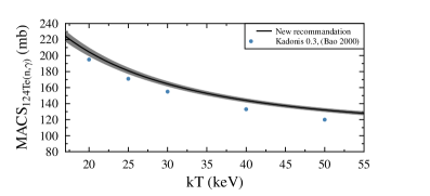
Figure 35: New and old WVK92 ; BBK00 ; DHK06 recommendation for the $MACS$ of ¹²⁴Te.

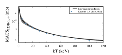
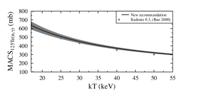
Figure 36: New and old WVK92 ; BBK00 ; DHK06 recommendation for the $MACS$ of ¹²⁵Te.

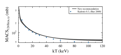
Figure 37: New and old WVK92 ; BBK00 ; DHK06 recommendation for the $MACS$ of ¹²⁶Te.

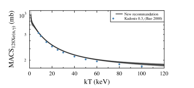
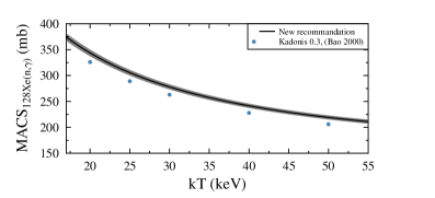
Figure 38: New and old RHK02 ; BBK00 ; DHK06 recommendation for the $MACS$ of ¹²⁸Xe.

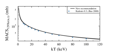
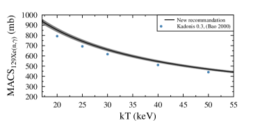
Figure 39: New and old RHK02 ; BBK00 ; DHK06 recommendation for the $MACS$ of ¹²⁹Xe.

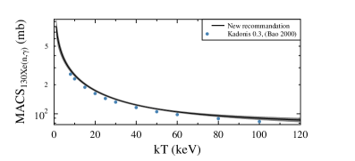
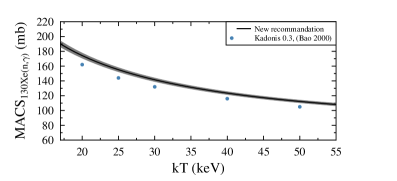
Figure 40: New and old RHK02 ; BBK00 ; DHK06 recommendation for the $MACS$ of ¹³⁰Xe.

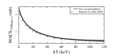
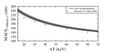
Figure 41: New and old VWG94b ; BBK00 ; DHK06 recommendation for the $MACS$ of ¹³⁴Ba.

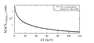
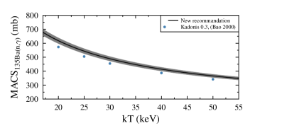
Figure 42: New and old VWG94b ; BBK00 ; DHK06 recommendation for the $MACS$ of ¹³⁵Ba.

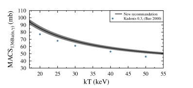
Figure 43: New and old VWG94b ; BBK00 ; DHK06 recommendation for the $MACS$ of ¹³⁶Ba.

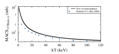
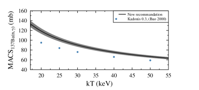
Figure 44: New and old VWG94b ; BBK00 ; DHK06 recommendation for the $MACS$ of ¹³⁷Ba.

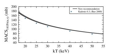
Figure 45: New and old VWA99 ; BBK00 ; DHK06 recommendation for the $MACS$ of ¹⁴¹Pr.

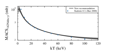
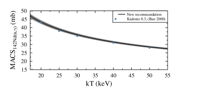
Figure 46: New and old WVK98a ; BBK00 ; DHK06 recommendation for the $MACS$ of ¹⁴²Nd.

Figure 47: New and old WVK98a ; BBK00 ; DHK06 recommendation for the $MACS$ of ¹⁴³Nd.

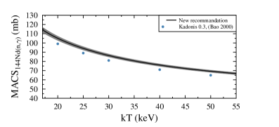
Figure 48: New and old WVK98a ; BBK00 ; DHK06 recommendation for the $MACS$ of ¹⁴⁴Nd.

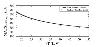
Figure 49: New and old WVK98a ; BBK00 ; DHK06 recommendation for the $MACS$ of ¹⁴⁵Nd.

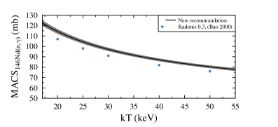
Figure 50: New and old WVK98a ; BBK00 ; DHK06 recommendation for the $MACS$ of ¹⁴⁶Nd.

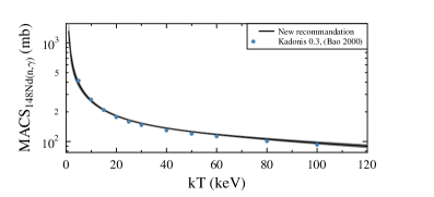
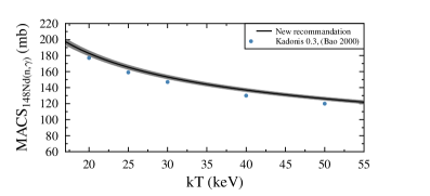
Figure 51: New and old WVK98a ; BBK00 ; DHK06 recommendation for the $MACS$ of ¹⁴⁸Nd.

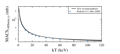
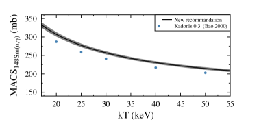
Figure 52: New and old WGV93 ; BBK00 ; DHK06 recommendation for the $MACS$ of ¹⁴⁸Sm.

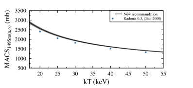
Figure 53: New and old WGV93 ; BBK00 ; DHK06 recommendation for the $MACS$ of ¹⁴⁹Sm.

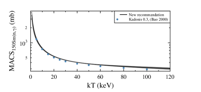
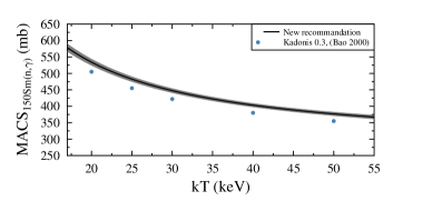
Figure 54: New and old WGV93 ; BBK00 ; DHK06 recommendation for the $MACS$ of ¹⁵⁰Sm.

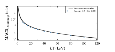
Figure 55: New and old WVK06 ; BBK00 ; DHK06 recommendation for the $MACS$ of ¹⁵¹Sm. The re-normalized values are in very good agreement with the TOF measurement performed at n_TOF AAA04 .

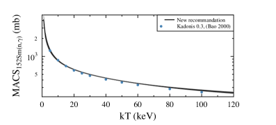
Figure 56: New and old WGV93 ; BBK00 ; DHK06 recommendation for the $MACS$ of ¹⁵²Sm.

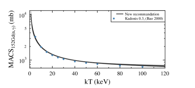
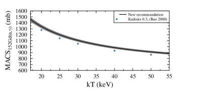
Figure 57: New and old WVK95b ; BBK00 ; DHK06 recommendation for the $MACS$ of ¹⁵²Gd.

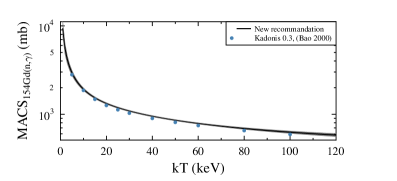
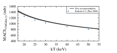
Figure 58: New and old WVK95b ; BBK00 ; DHK06 recommendation for the $MACS$ of ¹⁵⁴Gd.

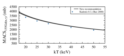
Figure 59: New and old WVK95b ; BBK00 ; DHK06 recommendation for the $MACS$ of ¹⁵⁵Gd.

Figure 60: New and old WVK95b ; BBK00 ; DHK06 recommendation for the $MACS$ of ¹⁵⁶Gd.

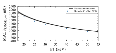
Figure 61: New and old WVK95b ; BBK00 ; DHK06 recommendation for the $MACS$ of ¹⁵⁷Gd.

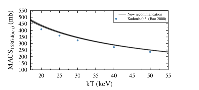
Figure 62: New and old WVK95b ; BBK00 ; DHK06 recommendation for the $MACS$ of ¹⁵⁸Gd.

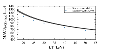
Figure 63: New and old VWA99 ; BBK00 ; DHK06 recommendation for the $MACS$ of ¹⁶⁰Dy.

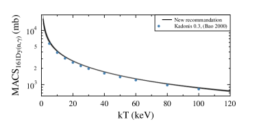
Figure 64: New and old VWA99 ; BBK00 ; DHK06 recommendation for the $MACS$ of ¹⁶¹Dy.

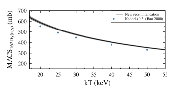
Figure 65: New and old VWA99 ; BBK00 ; DHK06 recommendation for the $MACS$ of ¹⁶²Dy.

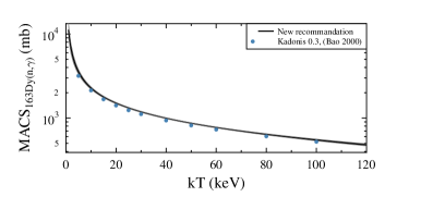
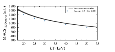
Figure 66: New and old VWA99 ; BBK00 ; DHK06 recommendation for the $MACS$ of ¹⁶³Dy.

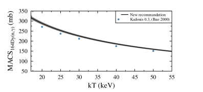
Figure 67: New and old VWA99 ; BBK00 ; DHK06 recommendation for the $MACS$ of ¹⁶⁴Dy.

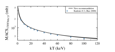
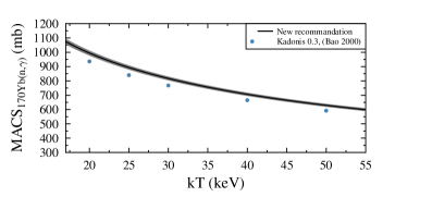
Figure 68: New and old WVA00a ; BBK00 ; DHK06 recommendation for the $MACS$ of ¹⁷⁰Yb.

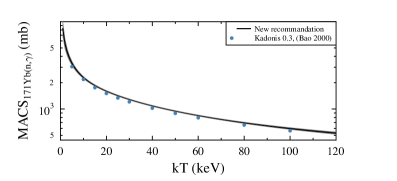
Figure 69: New and old WVA00a ; BBK00 ; DHK06 recommendation for the $MACS$ of ¹⁷¹Yb.

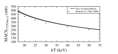
Figure 70: New and old WVA00a ; BBK00 ; DHK06 recommendation for the $MACS$ of ¹⁷²Yb.

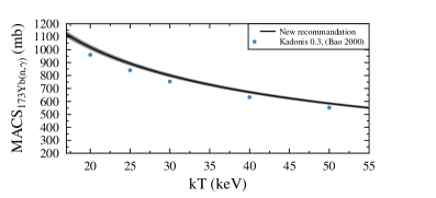
Figure 71: New and old WVA00a ; BBK00 ; DHK06 recommendation for the $MACS$ of ¹⁷³Yb.

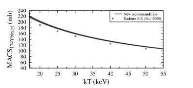
Figure 72: New and old WVA00a ; BBK00 ; DHK06 recommendation for the $MACS$ of ¹⁷⁴Yb.

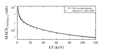
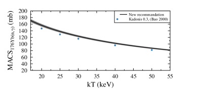
Figure 73: New and old WVA00a ; BBK00 ; DHK06 recommendation for the $MACS$ of ¹⁷⁶Yb.

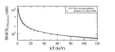
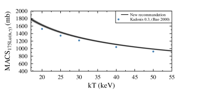
Figure 74: New and old WVK06b ; BBK00 ; DHK06 recommendation for the $MACS$ of ¹⁷⁵Lu.

Figure 75: New and old WVK06b ; BBK00 ; DHK06 recommendation for the $MACS$ of ¹⁷⁶Lu.

Figure 76: New and old WVK06c ; BBK00 ; DHK06 recommendation for the $MACS$ of ¹⁷⁶Hf.

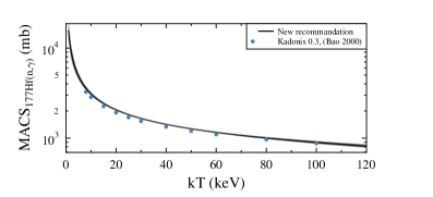
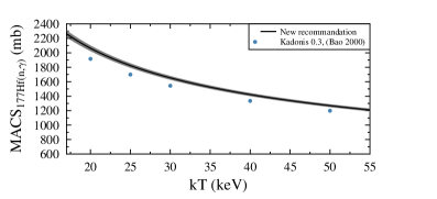
Figure 77: New and old WVK06c ; BBK00 ; DHK06 recommendation for the $MACS$ of ¹⁷⁷Hf.

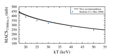
Figure 78: New and old WVK06c ; BBK00 ; DHK06 recommendation for the $MACS$ of ¹⁷⁸Hf.

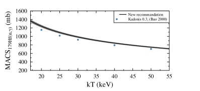
Figure 79: New and old WVK06c ; BBK00 ; DHK06 recommendation for the $MACS$ of ¹⁷⁹Hf.

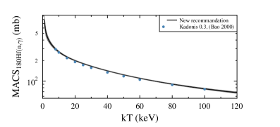
Figure 80: New and old WVK06c ; BBK00 ; DHK06 recommendation for the $MACS$ of ¹⁸⁰Hf.

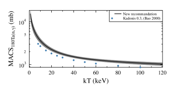
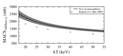
Figure 81: New and old WVA04 ; BBK00 ; DHK06 recommendation for the $MACS$ of ¹⁸⁰Ta.

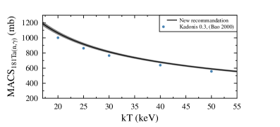
Figure 82: New and old WVK90 ; BBK00 ; DHK06 recommendation for the $MACS$ of ¹⁸¹Ta.

References

- (1) R. Reifarth, C. Lederer, F. Käppeler, Journal of Physics G Nuclear Physics 41, 053101 (2014)
- (2) A. Koloczek, B. Thomas, J. Glorius, R. Plag, M. Pignatari, R. Reifarth, C. Ritter, S. Schmidt, K. Sonnabend, Atomic Data and Nuclear Data Tables 108, 1 (2016)
- (3) C.J. Horowitz, A. Arcones, B. Cote, I. Dillmann, W. Nazarewicz, I.U. Roederer, H. Schatz, A. Aprahamian, D. Atanasov, A. Bauswein et al., Journal of Physics G submitted, https://arxiv.org/abs/1805.04637 (2018)
- (4) R. Surman, J. Engel, Phys. Rev. C 64, 035801 (2001)
- (5) K. Göbel, J. Glorius, A. Koloczek, M. Pignatari, R. Reifarth, R. Schach, K. Sonnabend, EPJ Web of Conferences 93, 03006 (2015)
- (6) T. Rauscher, F.K. Thielemann, Atomic Data Nucl. Data Tables 75, 1 (2000)
- (7) R. Reifarth, S. Dababneh, M. Heil, F. Käppeler, R. Plag, K. Sonnabend, E. Uberseder, Phys. Rev. C 85, 035802 (2012)
- (8) S. Schmidt, T. Heftrich, J. Glorius, G. Hampel, R. Plag, R. Reifarth, Z. Slavkovská, K. Sonnabend, C. Stieghorst, N. Wiehl et al., Nuclear Instruments and Methods in Physics Research A 768, 192 (2014)
- (9) R. Reifarth, C. Arlandini, M. Heil, F. Käppeler, P. Sedychev, A. Mengoni, M. Herman, T. Rauscher, R. Gallino, C. Travaglio, Astrophysical Journal 582, 1251 (2003)
- (10) E. Uberseder, R. Reifarth, D. Schumann, I. Dillmann, C.D. Pardo, J. Görres, M. Heil, F. Käppeler, J. Marganiec, J. Neuhausen et al., Physical Review Letters 102, 151101 (2009)
- (11) R. Reifarth, K. Schwarz, F. Käppeler, Ap. J. 528, 573 (2000)
- (12) M. Heil, F. Käppeler, M. Wiescher, A. Mengoni, Ap. J. 507, 997 (1998)
- (13) H. Nassar, M. Paul, I. Ahmad, D. Berkovits, M. Bettan, P. Collon, S. Dababneh, S. Ghelberg, J.P. Greene, A. Heger et al., Physical Review Letters 94, 092504 (2005)
- (14) H. Beer, G. Rupp, G. Walter, F. Voss, F. Käppeler, Nucl. Instr. Meth. A 337, 492 (1994)
- (15) R. Reifarth, M. Heil, C. Forssén, U. Besserer, A. Couture, S. Dababneh, L. Dörr, J. Görres, R.C. Haight, F. Käppeler et al., Phys. Rev. C 77, 015804 (2008)
- (16) R. Reifarth, F. Käppeler, Phys. Rev. C (Nuclear Physics) 66, 054605 ( 9) (2002)
- (17) N. Colonna, F. Gunsing, F. Käppeler, Progress in Particle and Nuclear Physics in press, https://doi.org/10.1016/j.ppnp.2018.02.002 (2018)
- (18) M. Tessler, M. Paul, A. Arenshtam, G. Feinberg, M. Friedman, S. Halfon, D. Kijel, L. Weissman, O. Aviv, D. Berkovits et al., Physics Letters B 751, 418 (2015)
- (19) C. Wiesner, L.P. Chau, H. Dinter, M. Droba, M. Heilmann, N. Joshi, D. Mader, A. Metz, O. Meusel, I. Müller et al., AIP Conference Proceedings 1265, 487 (2010)
- (20) R. Reifarth, L.P. Chau, M. Heil, F. Käppeler, O. Meusel, R. Plag, U. Ratzinger, A. Schempp, K. Volk, PASA 26, 255 (2009)
- (21) Z.Y. Bao, H. Beer, F. Käppeler, F. Voss, K. Wisshak, T. Rauscher, Atomic Data Nucl. Data Tables 76, 70 (2000)
- (22) W. Ratynski, F. Käppeler, Phys. Rev. C 37, 595 (1988)
- (23) H. Beer, F. Käppeler, Phys. Rev. C 21, 534 (1980)
- (24) R. Reifarth, M. Heil, F. Käppeler, R. Plag, Nucl. Inst. Meth. A 608, 139 (2009)
- (25) R. Auble, Nucl. Data Sheets 40, 301 (1983)
- (26) H. Liskien, A. Paulsen, Atomic Data and Nucl. Data Tables 15, 57 (1975)
- (27) C.L. Lee, X.L. Zhou, Nuclear Instruments and Methods in Physics Research B 152, 1 (1999)
- (28) M. Barbagallo, J. Andrzejewski, M. Mastromarco, J. Perkowski, L.A. Damone, A. Gawlik, L. Cosentino, P. Finocchiaro, E.A. Maugeri, A. Mazzone et al., Nuclear Instruments and Methods in Physics Research A 887, 27 (2018), 1708.01178
- (29) M. Heil, F. Käppeler, E. Uberseder, R. Gallino, M. Pignatari, Phys. Rev. C 77, 015808 (2008)
- (30) M. Weigand, C. Beinrucker, A. Couture, S. Fiebiger, M. Fonseca, K. Göbel, M. Heftrich, T. Heftrich, M. Jandel, F. Käppeler et al., Phys. Rev. C 95, 015808 (2017)
- (31) M. Moxon, E. Rae, Nucl. Instr. Meth. 24, 445 (1963)
- (32) K. Wisshak, F. Käppeler, Nucl. Sci. Engineering 66, 363 (1978)
- (33) K. Wisshak, F. Käppeler, Nucl. Sci. Engineering 69, 39 (1979)
- (34) F. Rau, Nukleonik 5, 191 (1963)
- (35) R. Macklin, J. Gibbons, Phys. Rev. 159, 1007 (1967), includes H. Maier-Leibnitz, priv. comm. and Rau63
- (36) P. Koehler, R. Winters, K. Guber, T. Rauscher, J. Harvey, S. Raman, R. Spencer, J. Blackmon, D. Larson, D. Bardayan et al., Phys. Rev. C 62, 055803 (2000)
- (37) K. Guber, L. Leal, R. Sayer, P. Koehler, T. Valentine, H. Derrien, J. Harvey, Nucl. Instr. Meth. B 241, 218 (2005)
- (38) R. Plag, M. Heil, F. Käppeler, P. Pavlopoulos, R. Reifarth, K. Wisshak, The N Tof Collaboration, Nuclear Instruments and Methods in Physics Research A 496, 425 (2003)
- (39) K. Wisshak, K. Guber, F. Käppeler, J. Krisch, H. Müller, G. Rupp, F. Voss, Nucl. Instr. Meth. A 292, 595 (1990)
- (40) C. Guerrero, U. Abbondanno, G. Aerts, H. Álvarez, F. Álvarez-Velarde, S. Andriamonje, J. Andrzejewski, P. Assimakopoulos, L. Audouin, G. Badurek et al., Nucl. Instr. Meth. A 608, 424 (2009)
- (41) M. Heil, R. Reifarth, M.M. Fowler, R.C. Haight, F. Käppeler, R.S. Rundberg, E.H. Seabury, J.L. Ullmann, J.B. Wilhelmy, K. Wisshak et al., Nucl. Instr. Meth. A 459, 229 (2001)
- (42) R. Reifarth, T.A. Bredeweg, A. Alpizar-Vicente, J.C. Browne, E.I. Esch, U. Greife, R.C. Haight, R. Hatarik, A. Kronenberg, J.M. O’Donnell et al., Nucl. Instr. Meth. A 531, 530 (2004)
- (43) G. Muradyan, A. Adamchuk, V. Adamchuk, Y. Shchepkin, M. Voskanyan, Nucl. Sci . Eng. 90, 60 (1985)
- (44) R. Block, Y. Danon, R. Slovacek, C. Werner, G. Youk, RPI NaI array, in Nuclear Data for Science and Technology, edited by J. Dickens (American Nuclear Society, La Grange Park, Illinois, 1994), p. 81
- (45) C. Guerrero, D. Cano-Ott, E. Mendoza, U. Abbondanno, G. Aerts, F. Álvarez-Velarde, S. Andriamonje, J. Andrzejewski, P. Assimakopoulos, L. Audouin et al., Phys. Rev. C85, 044616 (2012)
- (46) E.I. Esch, R. Reifarth, E.M. Bond, T.A. Bredeweg, A. Couture, S.E. Glover, U. Greife, R.C. Haight, A.M. Hatarik, R. Hatarik et al., Phys. Rev. C 77, 034309 (2008)
- (47) C. Wolf, J. Glorius, R. Reifarth, M. Weigand, Development of a detector in order to investigate (n,)-cross sections by ToF method with a very short flight path, in Journal of Physics Conference Series (2018), Vol. 940 of Journal of Physics Conference Series, p. 012060
- (48) R. Reifarth, S. Dababneh, S. Fiebiger, J. Glorius, K. Göbel, M. Heil, P. Hillmann, T. Heftrich, C. Langer, O. Meusel et al., Nuclear astrophysics at FRANZ, in Journal of Physics Conference Series (2018), Vol. 940 of Journal of Physics Conference Series, p. 012024
- (49) C. Guerrero, A. Tsinganis, E. Berthoumieux, M. Barbagallo, F. Belloni, F. Gunsing, C. Weiß, E. Chiaveri, M. Calviani, V. Vlachoudis et al., European Physical Journal A 49, 27 (2013)
- (50) A. Couture, R. Reifarth, Atomic Data and Nuclear Data Tables 93, 807 (2007)
- (51) R. Reifarth, R.C. Haight, M. Heil, F. Käppeler, D.J. Vieira, Nucl. Instr. Meth. A 524, 215 (2004)
- (52) A.D. Carlson, V. Pronyaev, G.M. Hale, C. Zhenpeng, R. Capote, I. Duran, F.J. Hambsch, T. Kawano, S. Kunieda, W. Mannhart et al., A new evaluation of the neutron data standards, in European Physical Journal Web of Conferences (2017), Vol. 146 of European Physical Journal Web of Conferences, p. 02025
- (53) S. Badikov, C. Zhenpeng, A. Carlson, E. Gai, G. Hale, F.J. Hambsch, H. Hofmann, T. Kawano, N. Larson, V. Pronyaev et al., Tech. rep., IAEA Vienna (2007)
- (54) A.D. Carlson, V.G. Pronyaev, D.L. Smith, N.M. Larson, Z. Chen, G.M. Hale, F.J. Hambsch, E.V. Gai, S.Y. Oh, S.A. Badikov et al., Nuclear Data Sheets 110, 3215 (2009)
- (55) P. Schillebeeckx, B. Becker, Y. Danon, K. Guber, H. Harada, J. Heyse, A.R. Junghans, S. Kopecky, C. Massimi, M.C. Moxon et al., Nuclear Data Sheets 113, 3054 (2012)
- (56) Z. Chunmei, Nuclear Data Sheets 95, 59 (2002)
- (57) R. Macklin, Nucl. Sci. Eng. 79, 265 (1981)
- (58) C. Massimi, C. Domingo-Pardo, G. Vannini, L. Audouin, C. Guerrero, U. Abbondanno, G. Aerts, H. Álvarez, F. Álvarez-Velarde, S. Andriamonje et al., Phys. Rev. C81, 044616 (2010)
- (59) C. Lederer, N. Colonna, C. Domingo-Pardo, F. Gunsing, F. Käppeler, C. Massimi, A. Mengoni, A. Wallner, U. Abbondanno, G. Aerts et al., Phys. Rev. C83, 034608 (2011)
- (60) C. Massimi, B. Becker, E. Dupont, S. Kopecky, C. Lampoudis, R. Massarczyk, M. Moxon, V. Pronyaev, P. Schillebeeckx, I. Sirakov et al., European Physical Journal A 50, 124 (2014)
- (61) G. Feinberg, M. Friedman, A. Krása, A. Shor, Y. Eisen, D. Berkovits, D. Cohen, G. Giorginis, T. Hirsh, M. Paul et al., Phys. Rev. C85, 055810 (2012)
- (62) C. Lederer, F. Käppeler, M. Mosconi, R. Nolte, M. Heil, R. Reifarth, S. Schmidt, I. Dillmann, U. Giesen, A. Mengoni et al., Phys. Rev. C85, 055809 (2012)
- (63) M.B. Chadwick, M. Herman, P. Obložinský, M.E. Dunn, Y. Danon, A.C. Kahler, D.L. Smith, B. Pritychenko, G. Arbanas, R. Arcilla et al., Nuclear Data Sheets 112, 2887 (2011)
- (64) NEA/EFF, working, group, Tech. rep., JEFF Report 19, OECD Nuclear Energy Agency, www.nea.fr/html/dbdata/nds_jefreports/jefreport-19/jefreport-19.pdf (2005)
- (65) A. Koning, C. Dean, U. Fischer, R. Mills, Tech. rep., JEFF Report 23, OECD Nuclear Energy Agency, www.oecd-nea.org/dbdata/nds_jefreports/jefreport-23/nea7079-jeff23.pdf (2013)
- (66) K. Shibata, O. Iwamoto, T. Nakagawa, N. Iwamoto, A. Ichihara, S. Kunieda, S. Chiba, K. Furutaka, N. Otuka, T. Ohasawa et al., Journal of Nuclear Science and Technology 48, 1 (2011)
- (67) F. Käppeler, R. Gallino, S. Bisterzo, W. Aoki, Reviews of Modern Physics 83, 157 (2011)
- (68) T. Rauscher, AIP Advances 4, 041012 (2014)
- (69) R. Macklin (1982), private communication to Mughabghab, S.F.
- (70) R. Capote (2018), private communication
- (71) I. Dillmann, M. Heil, F. Käppeler, R. Plag, T. Rauscher, F.K. Thielemann, KADoNiS- The Karlsruhe Astrophysical Database of Nucleosynthesis in Stars, in Capture Gamma-Ray Spectroscopy and Related Topics, edited by A. Woehr, A. Aprahamian (2006), Vol. 819 of American Institute of Physics Conference Series, pp. 123–127
- (72) K. Wisshak, F. Voss, C. Arlandini, F. Käppeler, L. Kazakov, Phys. Rev. C 61, 065801 (2000)
- (73) K. Wisshak, F. Voss, C. Arlandini, F. Käppeler, M. Heil, R. Reifarth, M. Krticka, F. Bec̆vár̆, Phys. Rev. C (Nuclear Physics) 69, 055801 ( 12) (2004)
- (74) K. Wisshak, F. Voss, C. Arlandini, F. Bec̆vár̆, O. Straniero, R. Gallino, M. Heil, F. Käppeler, M. Krtic̆ka, S. Masera et al., Physical Review Letters 87, 251102 ( 4) (2001)
- (75) Z. Németh, F. Käppeler, G. Reffo, Ap. J. 392, 277 (1992)
- (76) H. Beer, R. Macklin, Phys. Rev. C 26, 1404 (1982)
- (77) K. Wisshak, F. Voss, F. Käppeler, L. Kazakov, G. Reffo, Phys. Rev. C 57, 391 (1998)
- (78) K. Wisshak, F. Voss, F. Käppeler, Phys. Rev. C 57, 3452 (1998)
- (79) J. Escher, L. Ahle, L. Bernstein, J. Church, F. Dietrich, C. Forssén, R. Hoffman, Nucl. Phys. A 758, 86 (2005)
- (80) C. Forssén, F.S. Dietrich, J. Escher, R.D. Hoffman, K. Kelley, Physical Review C (Nuclear Physics) 75, 055807 (2007)
- (81) J. Escher, J. Burke, F. Dietrich, N. Scielzo, I. Thompson, W. Younes, Rev. Mod. Phys. 84, 353 (2012)
- (82) J.E. Escher, J.T. Burke, R.J. Casperson, R.O. Hughes, S. Ota, N.D. Scielzo, Capture cross sections from (p,d) reactions, in European Physical Journal Web of Conferences (2017), Vol. 146 of European Physical Journal Web of Conferences, p. 12014
- (83) G. Baur, C.A. Bertulani, H. Rebel, Nuclear Physics A 458, 188 (1986)
- (84) T. Nakamura, N. Fukuda, N. Aoi, N. Imai, M. Ishihara, H. Iwasaki, T. Kobayashi, T. Kubo, A. Mengoni, T. Motobayashi et al., Phys. Rev. C 79, 035805 (2009)
- (85) E. Uberseder, T. Adachi, T. Aumann, S. Beceiro-Novo, K. Boretzky, C. Caesar, I. Dillmann, O. Ershova, A. Estrade, F. Farinon et al., Physical Review Letters 112, 211101 (2014)
- (86) M. Heine, S. Typel, M.R. Wu, T. Adachi, Y. Aksyutina, J. Alcantara, S. Altstadt, H. Alvarez-Pol, N. Ashwood, L. Atar et al., Phys. Rev. C95, 014613 (2017)
- (87) K. Boretzky, B. Agrawal, G. Alkhazov, G. Andreev, T. Aumann, P. Basu, D. Bemmerer, D. Bertini, P. Bhattacharya, S. Bhattacharya et al., Tech. rep., GSI, Darmstadt (2011), gSI Sci. Rep., PHN-NUSTAR-NR-02, p. 174
- (88) K. Sonnabend, P. Mohr, K. Vogt, A. Zilges, A. Mengoni, T. Rauscher, H. Beer, F. Käppeler, R. Gallino, Ap. J. 583, 506 (2003)
- (89) H. Weller, Progress in Nuclear and Particle Physics 62, 257 (2008)
- (90) P.M. Hillenbrand, S. Hagmann, T. Stöhlker, Y. Litvinov, C. Kozhuharov, U. Spillmann, V. Shabaev, K. Stiebing, M. Lestinsky, A. Surzhykov et al., Physica Scripta Volume T 156, 014087 (2013)
- (91) R. von Hahn, F. Berg, K. Blaum, J.R. Crespo Lopez-Urrutia, F. Fellenberger, M. Froese, M. Grieser, C. Krantz, K.U. Kühnel, M. Lange et al., Nuclear Instruments and Methods in Physics Research B 269, 2871 (2011)
- (92) R. Reifarth, Y.A. Litvinov, Phys. Rev. ST Accel. Beams 17, 014701 (2014)
- (93) R. Reifarth, K. Göbel, T. Heftrich, M. Weigand, B. Jurado, F. Käppeler, Y.A. Litvinov, Phys. Rev. Accel. Beams 20, 044701 (2017)
- (94) R. Reifarth, D. Brown, S. Dababneh, Y.A. Litvinov, S.M. Mosby, Jordan Journal of Physics 11, 27 (2018)
- (95) K. Wisshak, F. Voss, F. Käppeler, G. Reffo, Phys. Rev. C 42, 1731 (1990)
- (96) K. Wisshak, F. Voss, F. Käppeler, L. Kazakov, Phys. Rev. C66, 025801 (2002)
- (97) K. Wisshak, F. Voss, C. Theis, F. Käppeler, K. Guber, L. Kazakov, N. Kornilov, G. Reffo, Phys. Rev. C 54, 1451 (1996)
- (98) K. Wisshak, F. Voss, F. Käppeler, G. Reffo, Phys. Rev. C 45, 2470 (1992)
- (99) R. Reifarth, M. Heil, F. Käppeler, F. Voss, K. Wisshak, F. Bec̆vár̆, M. Krtic̆ka, R. Gallino, Y. Nagai, Phys. Rev. C (Nuclear Physics) 66, 064603 ( 14) (2002)
- (100) F. Voss, K. Wisshak, K. Guber, F. Käppeler, G. Reffo, Phys. Rev. C 50, 2582 (1994)
- (101) F. Voss, K. Wisshak, C. Arlandini, F. Käppeler, L. Kazakov, T. Rauscher, Phys. Rev. C 59, 1154 (1999)
- (102) K. Wisshak, K. Guber, F. Voss, F. Käppeler, G. Reffo, Phys. Rev. C 48, 1401 (1993)
- (103) K. Wisshak, F. Voss, F. Käppeler, M. Krtička, S. Raman, A. Mengoni, R. Gallino, Phys. Rev. C 73, 015802 (2006)
- (104) U. Abbondanno, G. Aerts, F. Alvarez-Velarde, H. Alvarez-Pol, S. Andriamonje, J. Andrzejewski, G. Badurek, P. Baumann, F. Becvar, J. Benlliure et al. ((n-TOF Collaboration)), Physical Review Letters 93, 161103 (2004)
- (105) K. Wisshak, F. Voss, F. Käppeler, K. Guber, L. Kazakov, N. Kornilov, M. Uhl, G. Reffo, Phys. Rev. C 52, 2762 (1995)
- (106) K. Wisshak, F. Voss, F. Käppeler, L. Kazakov, Phys. Rev. C73, 015807 (2006)
- (107) K. Wisshak, F. Voss, F. Käppeler, L. Kazakov, F. Bečvář, M. Krtička, R. Gallino, M. Pignatari, Phys. Rev. C73, 045807 (2006)