Random walks avoiding their convex hull
with a finite memory
Francis Comets111NYU Shanghai and Université Paris Diderot, Mathématiques, case 7012, 75205 Paris Cedex 13, France;
comets@lpsm.parisMikhail V. Menshikov222Department of Mathematical Sciences, Durham University, South Road, Durham DH1 3LE, UK;
mikhail.menshikov,andrew.wade@durham.ac.ukAndrew R. Wade22footnotemark: 2
(1st March 2024)
Abstract
Fix integers and .
Consider a random walk in in which, given (),
the next step is uniformly distributed on the unit ball centred at , but
conditioned that the line segment from to intersects the convex hull
of only at .
For this is a version of the
model introduced by Angel et al., which is conjectured to be ballistic,
i.e., to have a limiting speed and a limiting direction. We establish
ballisticity for the finite- model, and comment on some open
problems. In the case where and , we obtain the limiting speed explicitly: it is
.
Key words: Random walk; convex hull; rancher; self-avoiding; ballistic; speed.
Random walks in Euclidean space whose evolution depends not just upon their most recent state
but upon their previous history have recently attracted much interest.
Such non-Markov processes arise naturally in systems where there is learning,
resource depletion, or physical interaction. For example,
a roaming animal performing a random walk may tend to avoid previously visited regions
to access new resources [25, §4]. Another major motivation is to provide models in polymer science, where linear chain molecules naturally appear both in collapsed and extended phases [2].
A broad class of models is provided by random walks (or diffusions) that interact with the occupation measure of
their
past trajectory. This interaction can be local, such for reinforced [21] or excited random walks [5], in which the walker’s
motion is biased by its occupation measure in the immediate vicinity,
or global, such as for processes with self-interaction mediated via some
global functional of the past trajectory, such as a centre of mass or other occupation statistic [4, 9, 18, 20, 26, 27, 28].
In either case, the self-interaction can be attractive, corresponding to the collapsed polymer phase,
or repulsive, corresponding to the extended phase.
An important distinction exists between dynamic models, that are genuine stochastic processes,
and static models, such as the self-avoiding walk [16], which is the extreme case in which repulsion is total.
Locally self-repelling walks in continuous space also appear in queueing theory, as models of customer-server systems with greedy strategies:
customers arrive randomly in time and space and the server moves toward the closest customer between services. Questions of interest include stability when the space is the circle [24], and transience and rate of escape on the line [12, 23]. Analogues in discrete space are considered in [10, 14],
where it is shown that in different regimes the server’s trajectories mimic either the self-avoiding or correlated random walk [8].
The inspiration for the work in the present paper originates with
a model of Angel et al. in which the random walk is forbidden from entering the
convex hull of its previous trajectory [1, 29].
This model, known as the rancher process, is believed to be ballistic (see below), but no proof of this exists at the moment.
A lattice-based model which shares some common features with the rancher process
is the prudent random walk [4] in which the walker avoids travelling in a direction towards a previously visited site.
It is worth noting that the scaling limits of the prudent walk in its kinetic version [4] and its static (uniform) version [7, 22] are quite different.
In this paper we consider a
variant of the rancher model in continuous space for which we can establish ballisticity.
Let us describe our model, a version of the rancher problem
which retains memory only of a fixed number of its recent locations together with its initial point (the origin). Fix (the ambient dimension)
and
(the length of the memory of the walk) with (this condition rules out degenerate cases, as we explain below).
Our object of interest is the stochastic process
in
where, roughly speaking, given , the next position
is uniformly distributed on the unit ball centred at
but conditioned so that the line segment from to does not intersect the convex hull of
at any point other than (which is necessarily on the boundary of the hull).
To give the formal definition,
we write for the convex hull of a subset , that is, the smallest
convex set containing .
Let denote the closed Euclidean -ball
centred at with radius , and
for let
, which for is the line segment from to excluding .
The set of admissible states from with history is
(1)
where taking the closure (‘’) is convenient for some measurability statements.
Let denote Lebesgue measure on ,
and set
.
We define the law of by taking
and declaring that, for ,
(2)
for all Borel sets , where is the transition density
defined for by
(3)
if ; i.e.,
given , the next step is uniform on .
We call the random walk with memory .
The definition is analogous to the ones in [1, 29] for the ‘infinite memory’ case.
See Figure 1 for an illustration in .
Lemma 2.1 below shows that we only need to define when
; hence the process is well defined.
Note that we do not allow . Indeed, in that case
has at most vertices,
so it is contained in a -dimensional hyperplane,
and is, up to a set of measure zero,
the whole of : the random walk has no interaction with its history, and has independent jumps.
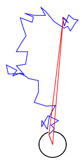
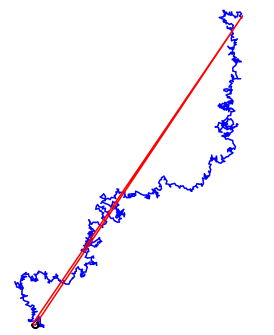
Figure 1: Simulation of the , process for steps (left)
and steps (right). The trajectory is in blue, the convex hull in red, and the black arc describes the disk sector on which the next position is distributed.
The main aim of this paper is to prove that this random walk is ballistic, i.e.,
it has a positive asymptotic speed and a limiting direction. Here is the theorem.
Write for the Euclidean norm on and set
.
Theorem 1.1.
There exist a positive
constant and a uniformly distributed such that
Note that including the origin in the definition of the convex hull to be
avoided at each step is crucial;
if the process instead just avoids the convex hull generated by its most recent steps, then it will be diffusive,
like the Gillis–Domb–Fisher ‘correlated random walk’ [8] that is repelled by its immediate past but effectively has zero drift
over long time scales. Another model whose dynamics, like ours, are influenced by both
its very distant and very recent past was considered recently by Gut and Stadtmüller [13] and is
a variant of the ‘elephant random walk’ [3, 6]. For their model on , Gut and Stadtmüller
obtain a ballisticty result reminiscent of Theorem 1.1: see Theorem 10.1 of [13].
The constants in Theorem 1.1 are characterized in (37) below, but seem hard to evaluate in general.
It is obvious that ,
and we show (cf. Corollary 2.8) that . It is likely that
one can show that for all , perhaps by adapting the arguments of [29];
this fact would also follow from Conjecture 1.3 below.
We can compute explicitly in one particular case.
Theorem 1.2.
If and , then
Simulations suggest the following.
Conjecture 1.3.
We have for all .
It is natural to seek a coupling to establish Conjecture 1.3. There is an obvious coupling
of one step of the and processes started from a common configuration, but extending this to a process coupling seems difficult.
The inspiration for considering our model comes
from the case of infinite memory,
when the walk avoids its entire convex hull
. This ‘’ walk is a variant of the model introduced by Angel et al. in [1],
in which the increments are uniform on the unit sphere
(rather than the unit ball)
excluding the convex hull;
for the case of that model, Zerner [29] showed that a.s.
Just as for the model in [1], one conjectures that the walk that avoids its entire convex hull is ballistic
(cf. Conjectures 1 and 5 in [1]);
in particular, one expects that exists.
Our Conjecture 1.3 would imply that exists. It is then tempting to propose the following.
Conjecture 1.4.
We have .
Simulations are reasonably consistent with Conjecture 1.4, but not entirely convincing.
Another open problem concerns the second-order behaviour of in the finite-memory model:
we expect that converges to a non-degenerate normal
distribution; this is to be contrasted with the conjectured -order fluctuations (in ) for the model [1]. It is also open to prove ballisticity for the version of the finite-memory model
(, say)
in which the increments are supported on a sphere rather than a ball:
our proof (particularly the renewal construction in Section 3) uses the fact that
the increments have a density in . In the case , of this variant of the model,
the argument
of Section 6 goes through with minor modifications to show that
The plan of the paper is as follows. In Section 2
we collect some initial observations, which include a
description of the process via a -component Markov chain
and the fact that there is a uniformly positive radial drift for the process
over a finite number of steps, which entails a -speed bound.
The core of our proof of ballisticity is a renewal structure described in Section 3,
which identifies events that occur frequently and between any two of which the process
has uniformly positive radial drift and has symmetric transverse increments. This is essentially already
enough to prove a limiting direction, but to identify a limiting speed it is necessary to show that
the radial drift between renewals has a limit, and that the expected time between renewals also has a limit.
We establish these limiting statements via a coupling argument to a
variant
of the process which is spatially homogeneous. The homogeneous process is introduced in Section 4,
and the coupling argument is presented in Section 5. This completes the proof of Theorem 1.1.
The proof of Theorem 1.2 proceeds via an essentially self-contained argument in Section 6, which shows that has the specified limit.
The argument goes by showing that the global speed is asymptotically equal to the local drift, and the local drift is evaluated as
an average with respect to the limit distribution of the interior angle of the convex hull;
the limit distribution of the angle is identified in
Lemma 6.3 as the limit of
the stochastic recursive sequence
taking values in , where are i.i.d. uniform.
The technical results required to deduce limiting speed and direction from statements about increments are collected in the Appendix.
2 Preliminaries
For any finite non-empty and
any , let
Excluding the degenerate case ,
is the convex hull of finitely many closed rays emanating from ,
and, if is not in the interior of , then is the smallest closed convex cone with vertex containing the set
(equivalently, ). It is not hard to see that (1) is equivalent to
(4)
which is a form that will be useful later on.
Our first result of this section shows that our process is well defined.
Here and subsequently, is the volume of the unit-radius
-ball.
Lemma 2.1.
The process is well defined, and for all , a.s.,
(5)
Proof.
The proof goes by induction.
Starting from
we have that by (1) or (4).
Hence ,
so (5) holds with .
For the inductive step, suppose that
the law of
is well defined, and that (5)
holds for all .
Then the transition density
at (3) is well-defined for , and so we can generate according to (2).
Thus is well defined: see Figure 2 for an example.
Moreover, the upper bound on
is trivial. Also, by construction, is not in the interior of the previous convex hull , and so is extremal
for . Hence there exists a tangent hyperplane at to the convex hull, and the opposite half of the ball is contained in
.
Hence the latter set has volume at least , and so (5)
holds for . This completes the inductive step.
∎
Figure 2: An illustration of the proof of Lemma 2.1 with . Left: the new point
sits outside
.
Right:
Indicated is half of the disc which falls outside the updated convex hull , giving a lower bound
on the area of .
For define
Let .
A sequence of points in is called an admissible path from history
if
,
,
,
and so on, up to
.
Let denote the set
of all admissible paths from history .
To describe the initial steps of the process,
we say is an admissible initial path
if , ,
, and so on, up to
.
Let denote the set
of all admissible initial paths.
The are Borel (in fact, closed) subsets of .
To see this,
take
with as .
Since is closed, .
Moreover, as a function taking values in the non-empty compact subsets of endowed with the Hausdorff metric (denoted ),
is continuous, and so
.
Given , we can (and do) choose sufficiently large so that
and .
Then since , there exists
with , so that . Hence ,
since the latter set is closed. Continuing this argument shows that ,
so the latter set is closed.
Similarly, is a closed subset of .
Lemma 2.2.
The process is a Markov process
on with transition function defined
for all Borel sets by
and elsewhere we set .
Moreover, the initial distribution is
where for all ,
Proof.
It suffices to suppose that for Borel sets in . By (2) and (3),
which gives the result if . Otherwise,
which gives the result if . Iterating this argument gives the transition function for general .
A similar argument gives the law of .
∎
For define the -algebra .
For , define .
For convenience, set . We write ‘’ for the scalar product on .
The following important result says that the radial component of the drift of the process
is always non-negative.
Proposition 2.3.
We have that, for all ,
Proof.
Given that , it suffices to suppose that , in which case , a.s. On the event , for ,
by (2) and (3) we can write
where the open set
(7)
differs from as given by (4)
by a set of measure zero (‘’ stands for ‘interior’).
For , define , the orthogonal transformation of
induced by reflection in the hyperplane at orthogonal to . We claim that
(8)
Write
and . Then by (8) and the fact that
, we have
and, using also the fact that is a measure-preserving bijection,
(9)
Hence, partitioning into and , we get
(10)
using (9). Moreover, the integrand in the final integral in (2)
is positive, by definition of . Thus we conclude that the final integral in (2)
is non-negative.
It remains to prove the claim (8). To do so, we use a finite-dimensional version of Hahn–Banach theorem:
for all , there exists a hyperplane separating and
such that and
here it is important that we used defined at (7).
Consider the unit vector perpendicular to and such that , and denote by the half-spaces
Then, for and , we have
and though . Since also ,
we have from (7) that . Thus
we have proved (8).
∎
We would like to improve Proposition 2.3 to show that the radial drift
is uniformly positive. However, it is not hard to see that there are configurations
for which this is not true if we compute the drift in a single step. Thus we are led to consider multiple steps.
In order to control the possible configurations of the walk’s history, we can demand that the walk first
makes a chain of jumps away from the convex hull, and then makes another chain of jumps in the radial direction.
These two constructions will be central to our renewal structure that we describe in the next section,
and they are the focus of the next two results.
For , , and any unit vector ,
define
(11)
Given , consider a tangent hyperplane at to , and
let be the perpendicular unit vector to this hyperplane, pointing opposite to
the convex hull.
We show that from any configuration, the walk will follow the chain laid out by
with uniformly positive probability.
Lemma 2.4.
We have that
Proof.
Suppose that ; note that .
Let for .
Define the events .
It is easy to see that .
Hence, by (2) and (3),
(12)
by Lemma 2.1. If , this completes the proof. In general, we claim that
(13)
Then, for instance,
by (12) and (13). Iterating this argument proves the statement in the lemma.
It remains to prove the claim (13).
For , consider the hyperplane .
Any has , and,
for , , while . Hence lies on , and the hyperplane separates
and all the , , from .
Thus, on .
The claim (13) follows.
∎
With the notation at (11), define
.
The key to our renewal structure is the following definition:
(14)
For , let denote the event ;
if occurs, we say that has good geometry at time .
Roughly speaking,
the process has good geometry if the configuration is such that, in the next steps,
all trajectories through the
sequence of balls laid out by are admissible.
More precisely, the next result shows that, if the process has good geometry, then
the law of the next steps has a uniform component on
the balls laid out by .
Lemma 2.5.
For all and all Borel , on the event ,
Proof.
For suppose that ,
where for Borel subsets of .
On the event , we have that .
In particular, ,
so that, by (2) and (3) we have,
on ,
If this ends the proof. Otherwise, on ,
we have that ,
so that
as before. Hence, on ,
Iterating this argument gives the result.
∎
Recall the definition of from just before Lemma 2.4.
The connection between the last two lemmas is the following.
Lemma 2.6.
We have that implies .
Proof.
Suppose that . Let .
Let . We must show that .
For convenience, set
for , and set
for .
It is not hard to see that .
We have for ,
and where .
For , consider the hyperplane .
Then so .
For all we have ,
so .
Also, for we have ,
while .
Thus contains and separates
and any , , from .
In particular, for , this
shows that , and so on.
∎
Now we can state our result on positive radial drift over a number of steps.
Proposition 2.7.
Suppose that and .
Then there exists a constant with such that, for all ,
(15)
Proof.
We will show that there exist
constants (depending on and ) and an event ,
such that
(16)
(17)
Note that for all ,
,
so .
Hence, by Proposition 2.3,
which is bounded below by , by the claims (16) and (17). This gives (15) with .
The rest of the proof establishes (16) and (17).
We describe the event , which will comprise three successive events.
Given , let be the perpendicular unit vector to a tangent hyperplane at to ,
pointing opposite to
the convex hull.
Define the events
and .
Then by Lemmas 2.4, 2.5, and 2.6,
we have that , a.s.
Suppose that occurs and consider the situation at time .
Let for ,
and let .
On , we have .
Set ,
and let
be an orthonormal basis for containing .
Next set
and let
for .
The idea is that, with positive probability, the process
will follow close to the path ,
at which point it will have strictly positive drift after producing a convex hull which
contains, approximately, a simplex.
Set for .
Define the events
Then, on , . Suppose that
is small enough so that .
Define hyperplanes .
First note that and, for ,
,
while ,
so the hyperplane contains and separates
from . So, on ,
we have . Now suppose that
and that occurs.
For ,
given , we have, noting that and ,
provided that .
Similarly, for , given ,
On the other hand,
Thus the hyperplane contains and separates
and from .
Hence, on , we have that .
Setting , it follows that
as required for (16).
It remains to prove (17), i.e., to show that on there is a uniformly positive radial drift.
As above, let where .
Also let .
Define the simplex to be the convex polytope with
vertices .
Define the barycentre of the vertices .
Note that , and so
Since , it follows that
Let denote the ‘approximate simplex’ with vertices .
Then on we have that while for .
Now is continuous as a function of and away from ,
so in particular we can choose small enough so that
(18)
where is the barycentre of the vertices of .
We claim that for small enough, is in the interior of .
Indeed, is in the interior of unless it degenerates to
a polytope of lower dimension. But is a continuous function of
its vertices, and the volume is strictly positive when (since then is a genuine simplex), so we can find
small enough so that the claim holds.
Hence, for small enough ,
and hence .
Setting and using analogous notation to the proof of
Proposition 2.3, we have
that . Hence from (2), on ,
by (18). This gives (17) with ,
and completes the proof.
∎
Having established a strictly positive radial drift, we can deduce that the
process has a positive ‘’ speed. This is the next result.
Corollary 2.8.
Suppose that and .
There exist constants and , depending only on and , such that
(19)
Moreover,
, a.s.
Proof.
Define the process . Then, since ,
Also, writing , we have
by (15). Hence is a submartingale
with uniformly bounded increments, and we can apply the one-sided
Azuma–Hoeffding inequality (see Theorem 2.4.14 in [17])
to obtain
Hence, since , for some depending on and , for all ,
(20)
Let .
Since , it follows that
for all sufficiently large. Then (20) yields (19).
Finally, it follows from (19) and the Borel–Cantelli lemma
that , a.s.
∎
3 Renewal structure
Our strategy for establishing ballisticity is to show that, up to smaller order terms,
there is a limiting positive radial drift and the transverse fluctuations are not too big (cf. Lemma A.1 below).
As in Proposition 2.7,
it is clear that this property cannot be the case at every step of the walk. Our strategy is to find an embedded process
which has these properties at random times. We call these random times ‘renewals’. They are such that process executes a chain
of approximately radial jumps (cf. Lemma 2.5). Such times exhibit a symmetry which entails a positive radial drift,
and these times occur rather frequently, as we show in Lemma 3.3 below. With Corollary 2.8,
this is already essentially enough to
establish a limiting direction. To establish a limiting speed, it is required in addition that the radial drift at these renewal
times, and the expected time between renewals, have limits; these quantities are not constant because the special rôle played by the origin means the process lacks homogeneity.
We address this with a coupling to a homogeneous modification of the process, which, roughly speaking, sends the origin away to infinity,
as described in Section 4.
From this point on, we fix the constant .
Recall the definition of from (11)
and of from (2.2). First we state
a consequence of Lemma 2.5.
Now we construct a version of which exhibits the required renewal structure,
by introducing an additional source of randomness
via a sequence
of i.i.d. Bernoulli random variables
with , where
is the constant in Corollary 3.1.
For now we call this new process
with ;
we will soon show that has the same law as .
The process will be adapted to the filtration
defined by .
At the same time as constructing the process, we generate a sequence of renewal times
as we shall describe.
Roughly speaking, is a renewal time if has good geometry at time and ; it allows a construction of the process such that its future evolution after a renewal
depends only on the current location , and not on the past.
Define the event .
To start with, we take to be distributed exactly as , as described in Lemma 2.2.
Given ,
suppose also that we have generated renewal times .
Then we generate as follows.
1.
If does not occur,
then generate from using the transition function described in Lemma 2.2.
2.
If does occur, then do the following.
(a)
If , then declare that is the next renewal time, and
set , where is the th component of
and the vector is uniformly distributed on .
(b)
If , then
set , where now is generated according to the density on
given by
(21)
where is defined at (2.2) and
is the constant in Corollary 3.1.
By Corollary 3.1,
as defined at (21)
is non-negative on , and
since, by Lemma 2.2,
where is the th component of ,
we have that, on ,
so is indeed a probability kernel.
Lemma 3.2.
The process has the same law as the process described at Lemma 2.2.
Proof.
By construction, has the same law as . Also by construction, we have that for Borel ,
(22)
on the complement of . It remains to show that (3) also holds on .
For Borel , we have
Since from we can recover , in view of Lemma 3.2, we will from now on work on an enlarged probability space
and assume that the process (and hence ) is constructed as , along with its renewal times.
We finish this section by showing that the renewal times must occur rather frequently.
Lemma 3.3.
With the constant appearing in Corollary 3.1, we have
(23)
Moreover, with given by , we have
(24)
Proof.
The statement (23) follows from Lemmas 2.4 and 2.6.
To prove (24), first note that is a stopping time for
for all .
Also, constructing and as described above, we have .
Let . Then by (23)
we have that, for all ,
Thus Lemma 3.3 shows that the sequence
does not terminate,
and its increments have exponentially bounded tails.
Consider the sequence . This is a Markov chain,
but its law is not translation invariant, due to the rôle of the origin.
The next section introduces a related process, whose increment law is translation invariant,
and which therefore has i.i.d. increments. In particular, it has a well-defined
radial drift which entails ballisticity, and, crucially, it is close enough in behaviour to to be able to deduce our theorems.
4 A homogeneous process
For any fixed vector we construct a homogeneous process in the direction . Loosely speaking, it amounts to replacing the origin by a point at infinity in the direction . Let us give a precise definition.
For , we consider a semi-infinite cylinder with direction ,
(26)
The set of -admissible states from
with history is
(27)
(28)
We start with an observation relating the admissible states.
Lemma 4.1.
Suppose that and . Then it holds that
(29)
Proof.
When , the origin belongs to , which is a convex set. Then and so comparison of (1) with (27) shows that .
Conversely,
consider the convex cone ;
the cone has vertex and contains , so that the translate ()
is contained in . That is, for any we have .
In other words,
is a convex cone that contains the cylinder ,
and hence .
Comparison of (4) and (28) shows that
, and the lemma is proved.
∎
We define the process
analogously to .
Specifically, we set ,
take , and suppose that, for ,
for all Borel sets , where
(30)
if .
This process is well defined, as shown by the following analogue
of Lemma 2.1; the proof is similar.
Lemma 4.2.
The process is well defined, and for all ,
A sequence is called an -admissible path from history
if
,
,
,
and so on, up to
.
Let denote the set
of all -admissible paths from history .
Let .
For and ,
recall from (11) that . Also, define
For , let denote the event ;
if occurs, we say that has good geometry at time .
The following analogue of Lemma 2.5 is proved in the same way.
Lemma 4.3.
Let be the constant appearing in Corollary 3.1.
Then for all and all Borel , on the event ,
For define
Now is a Markov chain and satisfies a version of Lemma 2.2.
Moreover, we may assume that is constructed along with its renewal
times , analogously to the construction of described
in Section 3,
with replacing , replacing ,
and replacing , where is defined by the analogue of (2.2)
with instead of , and
Let denote the th component of ,
and set .
Proposition 4.4.
The sequence is a homogeneous random walk,
that is,
is an i.i.d. sequence. Moreover,
and
for a constant which does not depend on . Finally,
the inter-renewal times
are i.i.d. with
for a constant depending only on and ,
and
such that, with the constant from Lemma 3.3,
(31)
Proof.
By the renewal construction and the
fact that for the -process the transition function is translation invariant,
where e.g. is the vector
with components . Thus is also i.i.d.
Similarly, are i.i.d., so that
does not depend on , and essentially the same argument as Lemma 3.3
gives the exponential bound (31).
Next observe that
The distribution of
is symmetric with respect to , i.e., invariant
under any orthogonal transformation of that leaves fixed.
Hence
for some , which does not depend on .
∎
5 Coupling the processes
In this section we describe a coupling construction used to approximate the process between times and
by the process , where is fixed as .
We simultaneously construct the processes and ,
and their subsequent renewal times,
essentially via the constructions described in Sections 3 and 4,
but with ‘maximal’ exploitation of common randomness.
Our primary process we again denote by ,
where , and we denote
in components, so the process yields the process .
Let denote the th component of , so .
Given (recall that is a stopping time), we will
generate ,
and, at the same time,
generate ,
where we couple the two processes and their renewal times in a maximal way (see below for formalities)
starting at
and using the same underlying sequence . We stress that is kept fixed.
Before describing the coupling formally, we recall the following fact (see e.g. [15, p. 19]):
If and are random variables on then there exists a maximal coupling, i.e., a law on
such that ,
where denotes total variation distance, which for measures and on is
defined by where the supremum is over
Borel sets .
Here is the coupling construction.
As before, let
be a sequence of i.i.d. Bernoulli random variables
with , where
is the constant in Corollary 3.1.
The joint construction of will be adapted to the filtration (thus we
enlarge the previous filtration as necessary).
Recall that and .
We begin by taking .
Let . If , we generate
and , and any associated renewal times, independently using
the constructions described previously in Sections 3 and 4.
If , then we generate and as follows.
1.
On the event ,
when neither process exhibits good geometry,
generate and via the maximal coupling of the corresponding marginal transition laws from .
2.
On the event , when both processes exhibit good geometry, then:
(a)
If ,
declare that a renewal occurs for both processes () and
set and where
and are generated via a maximal coupling of
the uniform laws on and , respectively. Generate the subsequent trajectories
of and independently.
(b)
If ,
set and where now
and are generated via a maximal coupling of
the laws
corresponding to the densities and .
3.
On the event (where ‘’ denotes the symmetric difference),
generate
and , and any associated renewal times, independently.
This construction gives for
with the correct marginal distributions.
Let denote the event that the coupling ‘succeeds’ between times and , i.e.,
(32)
The effectiveness of the coupling is based on the following result,
whose proof we defer to the end of this section. Write .
Proposition 5.1.
Let be as defined at (32).
There exists a constant such that a.s., for all but finitely many ,
The fact that the coupling succeeds with high probability leads to the following
key result, which quantifies how well the homogeneous process approximates the
real process between renewal times.
Corollary 5.2.
Let . Then the following hold.
(i)
Let be the constant appearing in Proposition 4.4.
Then, for all ,
(ii)
For all , there is a constant (depending on , , and ) such that
(iii)
Let be the constant appearing in Proposition 4.4.
Then, for all ,
Proof.
For part (i), with as defined at (32), we have that
Then, the (conditional) Hölder inequality implies that for all
with ,
(33)
for some constant and all but finitely many ,
by (24) and Proposition 5.1. In particular,
given ,
we may choose close enough to (and hence sufficiently large) so that this last bound is .
On the other hand, on the event we have where , so
where, similarly to above, , a.s.
Moreover, by Proposition 4.4, .
This establishes part (i).
To prove part (ii), observe first that, for all ,
(34)
Then the statement in part (ii) follows directly from (24).
For part (iii), we have that
Then (34) and an argument similar to (5) shows that
for all .
On the other hand, on the event we have where , so
where, again similarly to (5), we have that , a.s.
Moreover, by Proposition 4.4,
.
To compare
to ,
note that .
For with and , we have
(35)
Applying (35),
we see that
. Since a.s., we have
from the final statement in Corollary 2.8 that .
Part (iii) now follows.
∎
We can now complete the proof of Theorem 1.1. We use two results from the Appendix: Lemma A.3
which gives a law of large numbers for a process on under a drift and variance condition, and Lemma A.1
which implies ballisticity for a process on given suitable radial drift asymptotics and a speed bound.
By Corollary 5.2(i) and (24), we may apply Lemma A.3
with to obtain , a.s.
Moreover, by Corollary 5.2(ii) and (iii), we may apply Lemma A.1 to the process to obtain
for some random .
Let ,
so that .
Then by an inversion of the fact that ,
we obtain , a.s.
In particular, , a.s.
Then, since , we have
(36)
From (24) and the Borel–Cantelli lemma we have that there exists such that
,
for all but finitely many , a.s., and since this implies that
for all but finitely many , a.s.
Thus (36) yields
(37)
which is the required a.s. convergence result when we set .
The bounded convergence theorem yields ,
and the fact that follows from Corollary 2.8.
Finally, note that the law of is invariant
under orthogonal transformations of : for any orthogonal matrix , the sequence has the same law
as the original , and so the in (37) satisfies
, and the fact that is uniform on the sphere follows
from uniqueness of Haar measure.
∎
It remains to prove Proposition 5.1.
To establish this result we need the following observations.
We denote by the uniform law on measurable with .
Lemma 5.3.
There exists a constant such that, for any ,
(38)
There exists a constant such that for all and all
,
(39)
(40)
Moreover, there exists such that for all and all
,
(41)
Proof.
First it is straightforward to show that for measurable ,
(42)
In particular, the bound (38)
follows from (42)
and
the fact that ,
since the centres of and
are at distance at most .
Next we claim that there exists a constant such that for all , all and all of cardinality such that and have volume not smaller than ,
Moreover, it follows from (42) that there exists a constant such that for all with volume not smaller than ,
(44)
It remains to estimate the volume of
. Taking a parametrization of the segment from to , say , ,
we can control the derivative of the volume by the surface measure of the boundary of the admissible set,
(45)
But the set in (27) has a finite number of hyperplanar faces, uniformly bounded for a fixed . Since
has diameter less than , we conclude that the surface term is bounded, and further, that (43) holds.
We claim that (39) follows from (43).
Indeed, fix and
let be a random vector in
with
and let have the same distribution but with instead of .
To estimate we couple and component by component.
Then (43) shows that we can couple and such that . Given , the conditional densities of and
are and ,
respectively, so by (43) we may again couple so that . Iterating this argument yields
a coupling of and that fails with probability at most ,
which implies the total variation bound in (39).
Next, we claim that (40) follows from (38)
and (39). Indeed, by the definitions of and ,
which gives the result.
We now turn to the proof of (5.3). It is sufficient to consider the case .
We decompose
Here by (39).
For the other term we see from (44) that
where we have used the notation
It remains to prove that
(46)
for some constant .
For we simply use (45) to conclude (46). For general , we observe that
the set has a smooth boundary with bounded surface measure in . Then
By (24), we may (and do) choose sufficiently large so that , a.s.
The result now follows from the claim that there is a constant such that, for all and all ,
(47)
and the fact that, by Corollary 2.8, a.s. for some and all but finitely many ,
with the simple bound a.s.
It thus remains to prove the claim (47). Since for , we have
so to verify (47) it suffices to prove that, for all and all ,
Since and
, we thus obtain (48).
This completes the proof.
∎
6 The planar case with unit memory
This section is devoted to the proof of Theorem 1.2,
and so we take and throughout this section.
For , denote by the magnitude of the interior angle of at :
see Figure 3.
Figure 3: The definition of (left) and
the construction of (right).
In the right-hand diagram, the double-ruled angle is .
First we express the ‘local drift’ in terms of .
Lemma 6.1.
Let and . Then for ,
Proof.
Suppose that ; note that a.s.
Given and , let be polar coordinates
with origin at , in the direction ,
and oriented so that is at angle relative to .
See the left-hand part of Figure 3.
The area of the disk sector on which is uniformly distributed is
, so
which gives the result.
∎
Lemma 6.2.
Let and . Then for ,
where are i.i.d. random variables,
and a.s. as .
Proof.
Let .
Given and , once more use
the polar coordinates described in the proof of Lemma 6.1.
The angle
of in these coordinates
is , where ,
the angle between vectors and measured outside the convex hull,
is uniformly
distributed on ; say
for independent of . See the right-hand part of Figure 3.
The angle at
in the triangle with vertices
is ;
denote the angle at in by .
The angle at in is either
(if )
or (if ).
In the first case
and in the second case
Combining these we get
Since , it is not hard to see that ,
and this tends to since by Corollary 2.8.
∎
Lemma 6.3.
We have that
as
where has the distribution uniquely determined by the
distributional fixed-point equation
(49)
where is independent of the on the right.
Moreover, the random variable has probability density
given by
(50)
Remark 6.4.
It is not hard to check that (50) provides a solution to (49):
see the proof below, which also establishes uniqueness.
To come up with (50) in the first place, one can deduce
that the density of solving (49) satisfies the
differential equation
for all (by differentiating (54) below), and we observed that a linear solves this.
Then the fixed-point equation (49) reads , while
Lemma 6.2 shows that .
Let satisfy (49). Then clearly , a.s. Moreover,
for any ,
(51)
In particular, taking for , using the fact that and ,
so that and hence
. Thus any (finite)
solution to (49) has , a.s.
Define a Markov
transition operator on state-space by where , and measurable .
Then (49) is equivalent to the statement that
for all measurable , i.e.,
the distributional solutions to (49) are precisely the invariant measures of .
Note also that
so that for any measurable ,
where is uniform measure on .
This is a version of the Doeblin condition, and it ensures (see e.g. [19, Theorem 16.0.2, p. 394]) that is uniformly ergodic:
there is a unique invariant measure such that
as .
In particular (49) has a unique distributional solution.
Moreover, if denotes the set of probability measures on , then
(52)
Let denote the law of .
If is the Markov chain started from
and with evolution , then lives on the same probability space as ,
and has law .
Let denote the Lévy–Prokhorov metric on distributions.
Then
(53)
Here by (52) we can choose sufficiently large so that for all .
On the other hand,
we see that ,
so
which shows that .
Thus, since ,
for any we have , a.s.,
and so as .
Thus in (53) we may take both and large to see that
.
Thus converges in law to , the unique distributional solution to (49).
It remains to identify the law . To this end, we check that if has density as given by (50), then
(54)
which is . Hence provides a solution to
the distributional equation (49).
∎
Finally, we can complete the proof of Theorem 1.2.
By Lemmas 6.1 and 6.3 and the bounded convergence theorem,
where has the density given by (50). Then we compute
Comparison of Theorem 1.1 and Lemma A.5 shows that this quantity is
indeed , which ends the proof of Theorem 1.2.
∎
Appendix A Auxiliary results: speeds and directions
The next result, which will be our tool for establishing ballisticity,
is an important ingredient in the proof of Theorem 1.1.
Lemma A.1.
Let . Let be a stochastic
process in adapted to a filtration
. Let .
Suppose that a.s., for some constant ,
and that
for some , , and we have
(55)
(56)
Then a.s. for some random .
The proof of this result will go by establishing in turn a limiting speed (Lemma A.3)
and a limiting direction (Lemma A.4). First we need a couple of elementary bounds.
Lemma A.2.
For all ,
(57)
Moreover, for all with and ,
(58)
Proof.
First we prove (57). It suffices to suppose that .
We have
Let be a stochastic process on adapted to a filtration
. Suppose that there exist and such that
(61)
(62)
Then , a.s.
Proof.
As in the Doob decomposition, let and for ,
so that
is a martingale with . Moreover,
by (61). It follows that, for any ,
for all but finitely many , a.s.: to see this one may apply
e.g. Theorem 2.8.1 of [17] (take and in that result).
Hence, a.s.,
,
by (62).
∎
Lemma A.4.
Let . Let be adapted to a filtration
. Let .
Suppose that for some , (55) holds.
Let .
Suppose also that a.s., and,
for some ,
a.s.
Then a.s. for some random .
Proof.
First note that, by Markov’s inequality and (55), for any ,
(63)
On the other hand, we apply (58) with and to get, on ,
But for all but finitely many , so we get
, a.s.
It follows that a.s. for some , by e.g. the -dimensional
version of Theorem 5.4.9 of [11].
Hence for to converge a.s.,
it is sufficient that exists a.s., and, by (64),
sufficient for this is that
a.s.
Also, since , the limit of is non-zero.
∎
Taking and in (57), taking conditional expectations, and using (55), we obtain
Then by assumption (56) and the fact that for all but finitely many ,
So we can apply Lemma A.3 with to deduce that
, a.s. Moreover,
it also follows from (56)
that
, a.s. Hence the conditions of Lemma A.4
are also satisfied, and we conclude that a.s., for some .
Then , a.s.
∎
The next result, which shows how local speed translates to global speed, is an important
ingredient in the proof of Theorem 1.2.
Lemma A.5.
Let . Let be a stochastic
process in with , such that, for some constant ,
It follows from an application of (65) with and that
where . Since a.s.,
the bounded convergence theorem implies that , and the claimed result follows.
∎
Acknowledgements
F.C. and M.M. acknowledge the support of the project SWIWS (ANR-17-CE40-0032). The authors
are grateful to two anonymous referees for their comments and suggestions.
References
[1]
O. Angel, I. Benjamini, and B. Viràg,
Random walks that avoid their past convex hull.
Electron. Commun. Probab.8 (2003) 6–16.
[2]
M.N. Barber and B.W. Ninham,
Random and Restricted Walks: Theory and Applications.
Gordon and Breach, New York, 1970.
[3]
E. Baur and J. Bertoin,
Elephant random walks and their connection to Pólya-type urns.
Phys. Rev. E94 (2016) 052134.
[4]
V. Beffara, S. Friedli, and Y. Velenik,
Scaling limit of the prudent walk.
Electron. Commun. Probab.15 (2010) 44–58.
[5]
I. Benjamini and D.B. Wilson,
Excited random walk.
Electron. Commun. Probab.8 (2003) 86–92.
[6]
B. Bercu,
A martingale approach for the elephant random walk.
J. Phys. A: Math. Theor.81 (2018) 015201.
[7]
M. Bousquet-Mélou,
Families of prudent self-avoiding walks.
J. Combin. Theory Ser. A117 (2010) 313–344.
[8]
A. Chen and E. Renshaw,
The Gillis–Domb–Fisher correlated random walk.
J. Appl. Probab.29 (1992) 792–813.
[9]
F. Comets, M.V. Menshikov, S. Volkov, and A.R. Wade,
Random walk with barycentric self-interaction.
J. Stat. Phys.143 (2011) 855–888.
[10]
J.R. Cruise and A.R. Wade,
The critical greedy server on the integers is recurrent.
Ann. Appl. Probab.29 (2019) 1233–1261.
[11]
R. Durrett,
Probability: Theory and Examples.
4th ed.,
Cambridge University Press, Cambridge, 2010.
[12]
S. Foss, L. Rolla, and V. Sidoravicius,
Greedy walk on the real line.
Ann. Probab.43
(2015)
1399–1418.
[13]
A. Gut and U. Stadtmüller,
Variations of the elephant random walk. Preprint (2018),
arXiv:1812.01915.
[14]
I.A. Kurkova and M.V. Menshikov, Greedy algorithm, case.
Markov Process. Related Fields3
(1997)
243–259.
[15] T. Lindvall, Lectures on the Coupling Method.
John Wiley & Sons, Inc., New York, 1992.
[16]
N. Madras and G. Slade, The Self-Avoiding Walk.
Modern Birkhäuser Classics,
reprint of the 1993 original, 2013.
[17]
M. Menshikov, S. Popov, and A. Wade,
Non-homogeneous Random Walks.
Cambridge University Press, Cambridge, 2016.
[18]
T. Mountford and P. Tarrès, An asymptotic result for Brownian polymers.
Ann. Inst. H. Poincaré Probab. Statist.44
(2008)
29–46.
[19]
S.P. Meyn and R.L. Tweedie,
Markov Chains and Stochastic Stability.
2nd ed., Cambridge University Press, Cambridge, 2009.
[20]
J.R. Norris, L.C.G. Rogers, and D. Williams,
Self-avoiding random walk: A Brownian motion model with local time drift.
Probab. Theory Related Fields74 (1987) 271–287.
[21]
R. Pemantle,
A survey of random processes with
reinforcement.
Probab. Surv.4 (2007) 1–79.
[22]
N. Pétrélis, R. Sun, and N. Torri,
Scaling limit of the uniform prudent walk.
Electron. J. Probab.22 (2017)
paper no. 66, 19 pp.
[23]
L. Rolla and V. Sidoravicius,
Stability of the greedy algorithm on the circle.
Comm. Pure Appl. Math.70 (2017)
1961–1986.
[24]
L. Rolla, V. Sidoravicius, and L. Tournier,
Greedy clearing of persistent Poissonian dust.
Stochastic Process. Appl.124
(2014)
3496–3506.
[25]
P.E. Smouse, S. Focardi, P.R. Moorcroft, J.G. Kie, J.D. Forester and J.M. Morales,
Stochastic modelling of animal movement.
Phil. Trans. Roy. Soc. Ser. B Biol. Sci.365 (2010) 2201–2211.
[26]
B. Tóth,
The “true” self-avoiding walk with bond repulsion on : Limit theorems.
Ann. Probab.23 (1995) 1523–1556.
[27]
B. Tóth,
Self-interacting random motions—a survey.
In: Random Walks (Budapest, 1998)
Bolyai Soc. Math. Stud. 9 (1999)
349–384.
[28]
B. Tóth and W. Werner, The true self-repelling motion.
Probab. Theory Related Fields111
(1998)
375–452.
[29]
M. Zerner,
On the speed of a planar random walk avoiding its past convex hull.
Ann. Inst. H. Poincaré Probab. Statist.41 (2005) 887–900.