Calibration of gamma-ray bursts luminosity correlations using gravitational waves as standard sirens

Abstract

Gamma-ray bursts (GRBs) are a potential tool to probe high-redshift universe. However, the circularity problem enforces people to find model-independent methods to study the luminosity correlations of GRBs. Here, we present a new method which uses gravitational waves as standard sirens to calibrate GRB luminosity correlations. For the third-generation ground-based GW detectors (i.e., Einstein Telescope), the redshifts of gravitational wave (GW) events accompanied electromagnetic counterparts can reach out to $\sim 4$, which is more distant than type Ia supernovae ($z\lesssim 2$). The Amati relation and Ghirlanda relation are calibrated using mock GW catalogue from Einstein Telescope. We find that the $1\sigma$ uncertainty of intercepts and slopes of these correlations can be constrained to less than 0.2% and 8% respectively. Using calibrated correlations, the evolution of dark energy equation of state can be tightly measured, which is important for discriminating dark energy models.

1 Introduction

Gamma-ray burst (GRB) are one of the most energetic phenomena in our Universe (Kumar & Zhang, 2015; Wang, Dai & Liang, 2015). The high luminosity makes them detectable out to high redshifts. Therefore, GRBs are promising tool to probe the high-redshift universe: including the cosmic expansion and dark energy (Dai, Liang & Xu, 2004; Liang & Zhang, 2006; Schaefer, 2007; Wang, Dai & Zhu, 2007), star formation rate (Totani, 1997; Bromm, Coppi & Larson, 2002; Wang & Dai, 2009; Wang, 2013), the reionization epoch (Barkana & Loeb, 2004; Totani et al., 2006) and the metal enrichment history of the Universe (Wang et al., 2012; Hartoog et al., 2015). Among them, the $\gamma$-ray bursts correlations (for reviews, see Wang, Dai & Liang, 2015; Dainotti & Del Vecchio, 2017; Dainotti, Del Vecchio & Tarnopolski, 2018; Dainotti & Amati, 2018) are most widely studied, which can not only shed light on the radiation mechanism of GRBs, but also provide a promising tool to probe the cosmic expansion and dark energy (Wang, Dai & Liang, 2015; Dainotti & Del Vecchio, 2017). These correlations can be divided into three categories, such as prompt correlations, afterglow correlations and prompt-afterglow correlations. The prompt correlations mainly include Amati correlation (Amati et al., 2002), Ghirlanda correlation (Ghirlanda, Ghisellini & Lazzati, 2004), Liang-Zhang correlation (Liang & Zhang, 2005), Yonetoku correlation (Wei & Gao, 2003; Yonetoku et al., 2004) and $L_{\text{iso}}-\tau_{\text{lag}}$ correlation (Norris, Marani & Bonnell, 2000). Afterglow correlations contain only parameters in the afterglow phase, such as Dainotti correlation ($L_{X}(T_{a})-T^{*}_{X,a}$) (Dainotti, Cardone & Capozziello, 2008), $L_{X}(T_{a})-T^{*}_{X,a}$ and $L_{O}(T_{a})-T^{*}_{O,a}$ correlations (Ghisellini et al., 2009) and $L_{O,200\text{s}}-\alpha_{O,>200\text{s}}$ correlation (Oates et al., 2012). Prompt-afterglow correlations connect plateaus and prompt phases, referring to $E_{\gamma,\text{afterglow}}-E_{X,\text{prompt}}$ correlation (Liang, Zhang & Zhang, 2007), $L_{X,\text{afterglow}}-E_{\gamma,\text{prompt}}$ correlation (Berger, 2007), $L_{X}(T_{a})-L_{\gamma,\text{iso}}$ correlation (Dainotti, 2011), $L_{\text{iso}}-E_{\text{p},z}-\Gamma_{0}$ correlation (Liang et al., 2015) and so on.

However, there is a circularity problem when treating GRBs as relative standard candles. It arises from the derivation of quantities like luminosity $L_{\text{iso}}$, isotropic energy $E_{\text{iso}}$ and collimation-corrected energy $E_{\gamma}$, which are dependent on luminosity distance $d_{L}$ in a fiducial cosmology. For instance, the $d_{L}$ in a flat $\Lambda$CDM model can be expressed as

$$d_{L}(z)=\frac{c(1+z)}{H_{0}}\int_{0}^{z}\frac{\mathrm{d}z^{\prime}}{\sqrt{\Omega_{\text{m}}(1+z^{\prime})^{3}+(1-\Omega_{m}-\Omega_{\Lambda})(1+z^{\prime})^{2}+\Omega_{\Lambda}}}.$$ (1)

Therefore, it is inappropriate to use the model-dependent luminosity correlations to study cosmology models in turn. Several approaches have been proposed to overcome the problem (Wang, Dai & Liang, 2015; Dainotti & Del Vecchio, 2017). One method is to fit the cosmological parameters and luminosity correlation simultaneously (Ghirlanda et al., 2004; Li et al., 2008). Another method is to calibrate the correlations using type Ia supernovae (SNe Ia) (Liang et al., 2008) or observational Hubble Data (OHD) (Amati et al., 2018). It is based on the principle that objects of the same redshift should have same luminosity distance. Wang (2008) pointed out that the GRB luminosity correlations calibrated by SNe Ia are no longer completely independent of the SNe Ia data points. Consequently, the GRB data cannot be combined with the SNe Ia dataset directly to constrain cosmological parameters. What’s worse, high redshift SNe Ia can hardly be found and the furthest SN Ia yet seen is GND12Col with $z=2.26^{+0.02}_{-0.10}$ (Rodney et al., 2015), while the redshift of GRB can be up to 9.4 (Cucchiara et al., 2011). Moreover, there are many some systematic uncertainties for SNe Ia, such as dust in the light path (Avgoustidis, Verdec & Jimenez, 2009; Hu, Yu & Wang, 2017), the possible intrinsic evolution of SN luminosity, magnification by gravitational lensing (Holz, 1998), peculiar velocity (Hui & Greene, 2006), and so on. These processes will degrade the usefulness of SNe Ia as standard candles.

Here, we come up with the idea to calibrate GRB luminosity relations using gravitational waves (GW) standard sirens. The detection of GW170817 accompanied by electromagnetic counterparts heralds the new era of gravitational-wave multi-messenger astronomy (Abbott et al., 2017). Schutz (1986) first pointed out that the waveform signals from inspiralling compact binaries can be used to determine the luminosity distance to the source, serving as a standard siren. This kind of standard siren is a self-calibrating distance indicator, which just relying on the modelling of the two-body problem in general relativity (Sathyaprakash, Schutz & Van Den Broeck, 2010). The of detected BNS and BH-NS merger events can reach up to $z\sim 4$ to the farthest by Einstein Telescope (ET) (Abernathy et al., 2011; Li, 2015; Cai & Yang, 2017), going beyond the redshift limitation of SNe Ia. For the third generation detectors, such as ground-based Einstein Telescope (ET) (Abernathy et al., 2011), space-based Big Bang Observer (BBO) (Cutler & Holz, 2009), and Deci-Hertz Interferometer Gravitational wave Observatory (DECIGO) (Kawamura et al., 2011), smaller distance uncertainty will be achieved than Advanced LIGO and Virgo (Abbott et al., 2017).

The paper is organized as follows. In Section 2, we introduce the procedure of construction mock GW catalogue. The calibration of GRB luminosity correlations with GW standard sirens is illustrated in Section 3. A summary of our result and future outlooks is provided in the end of the paper.

2 Construction of GW standard sirens

2.1 Redshift distribution

In order to construct a mock GW catalogue, we need to consider the redshift distribution of the sources, which satisfies the following expression

$$P(z)\propto\frac{4\pi d_{C}^{2}(z)R(z)}{H(z)(1+z)},$$ (2)

where $d_{C}(z)$ is the comoving distance of the source. The time evolution of the NS-NS merger rate $R(z)$ is given by (Schneider et al., 2001)

$$R(z)=\begin{cases}1+2z,&z\leq 1\\ \frac{3}{4}(5-z),&1<z<5\\ 0,&z\geq 5.\end{cases}$$ (3)

The NS-NS merger rate at redshift $z$ is $\dot{n}(z)=\dot{n}_{0}\cdot R(z)$ and the merger rate today is about $\dot{n}_{0}=1.54^{+3.2}_{-1.22}\times 10^{-6}\text{ Mpc}^{-1}\text{ yr}^{-1}$ (Abbott et al., 2017).

2.2 Simulation of luminosity distances

It is necessary to define the total mass $M_{\text{phys}}=m_{1}+m_{2}$, symmetric mass ratio $\eta=\frac{m_{1}m_{2}}{M^{2}}$ and chirp mass $\mathcal{M}_{c,\text{obs}}=M\eta^{3/5}$ before our analysis, given binary component masses $m_{1}$ and $m_{2}$. The observed chirp mass is related to physical chirp mass via $\mathcal{M}_{c,\text{obs}}=(1+z)\mathcal{M}_{c,\text{phys}}$. Similarly, the observed total mass is $M_{\text{obs}}=(1+z)M_{\text{phys}}$.

2.2.1 Frequency domain waveform and Fourier Amplitude

The response of the detector $h(t)$ is a linear combination of two components

$$h(t)=F_{+}(\theta,\phi,\psi)h_{+}(t)+F_{\times}(\theta,\phi,\psi)h_{\times}(t),$$ (4)

where $F_{+}$ and $F_{\times}$ are the antenna pattern functions of the detector, $\psi$ is the polarization angle, and ($\theta,\phi$) is the location of the source on the sky. The antenna pattern functions of ET are

$$F_{+}^{(1)}(\theta,\phi,\psi) =\frac{{\sqrt{3}}}{2}\bigg{[}\frac{1}{2}(1+\cos^{2}\theta)\cos 2\phi\cos 2\psi-\cos\theta\sin 2\phi\sin 2\psi\bigg{]},$$ (5)

$$F_{\times}^{(1)}(\theta,\phi,\psi) =\frac{{\sqrt{3}}}{2}\bigg{[}\frac{1}{2}(1+\cos^{2}\theta)\cos 2\phi\sin 2\psi+\cos\theta\sin 2\phi\cos 2\psi\bigg{]}.$$

The other pattern functions are $F_{+,\times}^{(2)}(\theta,\phi,\psi)=F_{+,\times}^{(1)}(\theta,\phi+2\pi/3,\psi)$ and $F_{+,\times}^{(3)}(\theta,\phi,\psi)=F_{+,\times}^{(1)}(\theta,\phi+4\pi/3,\psi)$ respectively. The Fourier transform of time domain waveform $h(t)$ is given by

$$\mathcal{H}(f)=\mathcal{A}f^{-7/6}\exp(\text{i}(2\pi ft_{0}-\pi/4+2\psi(f/2)-\phi_{(2,0)})),$$ (6)

where

$$\mathcal{A}=\frac{1}{d_{L}}\sqrt{F^{2}_{+}(1+\cos^{2}\iota)^{2}+4F^{2}_{\times}\cos^{2}\iota}\sqrt{\frac{5\pi}{96}}\pi^{-7/6}\mathcal{M}_{c,\text{obs}}^{5/6}.$$ (7)

is the Fourier amplitude. The post-Newtonian formalism of GW waveform phase up to 3.5 PN is used (Blanchet et al., 2002) and the expressions of functions $\psi$ and $\phi_{(2,0)}$ can be found in Arun et al. (2005) and Zhao et al. (2011).

The component masses of binary neutron stars are randomly sampled in [1,2] $M_{\odot}$, while for neutron star-black hole systems, the component mass of black hole is uniform in [3,10] $M_{\odot}$ (Fryer & Kalogera, 2001; Li, 2015; Cai & Yang, 2017). The beaming angle of $\gamma$-ray bursts are randomly sampled in interval [0^∘,20^∘]. Since the GW signal-to-noise ratio in Sec. 2.2.2 is independent of the waveform phase, the $\psi$ and $\phi_{(2,0)}$ are not considered here.

2.2.2 The signal-to-noise ratio and estimated error

A GW signal is claimed to be detected only when combined signal-to-noise ratio (SNR) $\geq 8$ for a single detector network (Sathyaprakash, Schutz & Van Den Broeck, 2010). For ET, The combined SNR is

$$\rho=\sqrt{\sum_{i=1}^{3}(\rho^{(i)})^{2}},$$ (8)

where

$$\rho^{(i)}=\sqrt{\langle\mathcal{H}^{(i)},\mathcal{H}^{(i)}\rangle}.$$ (9)

and the bracket is defined by

$$\langle a,b\rangle=4\int_{f_{\text{min}}}^{f_{\text{max}}}\frac{a(f)b^{*}(f)+a^{*}(f)b(f)}{2}\frac{\mathrm{d}f}{S_{h}(f)}.$$ (10)

where $S_{h}(f)$ is the one-sided noise power spectrum density (PSD), which determines the performance of a GW detector. We take the noise PSD of ET to be

$$S_{h}(f)=S_{0}\bigg{[}x^{p_{1}}+a_{1}x^{p_{2}}+a_{2}\frac{1+b_{1}x^{1}+b_{2}x^{2}+b_{3}x^{3}+b_{4}x^{4}+b_{5}x^{5}+b_{6}x^{6}}{1+c_{1}x^{1}+c_{2}x^{2}+c_{3}x^{3}+c_{4}x^{4}}\bigg{]},$$ (11)

as in Zhao et al. (2011), where $x\equiv f/200$ Hz and $S_{0}=1.449\times 10^{52}$ Hz^-1. The parameters $p_{i}$, $a_{i}$, $b_{i}$ and $c_{i}$ are also provided in Zhao et al. (2011). The upper cutoff frequency $f_{\text{max}}$ is twice the orbit frequency at the last stable orbit, $f_{\text{max}}=2f_{\text{LSO}}=2/(6^{3/2}2\pi M_{\text{obs}})$. The lower cutoff frequency is $f_{\text{lower}}=1$ Hz.

At every simulated redshift, the fiducial value of the luminosity distance $d_{L}^{\text{fid}}$ is calculated according to Equation 1. Then we simulate the $\ln d_{L}^{\text{mea}}$ to be Gaussian distribution centered around $\ln d_{L}^{\text{fid}}$ with standard deviation $\sigma_{\ln d_{L}}$,

$$\ln d_{L}^{\text{mea}}=\mathcal{N}(\ln d_{L}^{\text{fid}},\sigma_{\ln d_{L}}).$$ (12)

The fiducial cosmology is flat $\Lambda$CDM cosmology with $\Omega_{\text{m}}=0.308,H_{0}=67.8\text{ km}\text{ s}^{-1}\text{ Mpc}^{-1}$ (Planck collaboration, 2016) when calculating $\ln d_{L}^{\text{fid}}$.

The Fisher matrix $\Gamma_{ij}$ is widely used to estimate the errors in the measured parameters,

$$\Gamma_{ij}=\bigg{\langle}\frac{\partial\mathcal{H}}{\partial p_{i}},\frac{\partial\mathcal{H}}{\partial p_{j}}\bigg{\rangle}.$$ (13)

where $p_{i}$ denotes the parameters on which the waveforms are depending, namely $(\ln\mathcal{M}_{c},\ln\eta,t_{0},\Phi_{0},\cos\iota,\psi,\ln d_{L})$. Then the estimated error $\sigma_{p_{i}}$ of parameter $p_{i}$ is $(\Gamma^{-1})_{ii}^{1/2}$. However, for calculation simplicity, we follow Cai & Yang (2017) and take the distance uncertainty $\sigma^{\text{inst}}_{d_{L}}$ to be $2d_{L}/\rho$, allowing for the correlation between $d_{L}$ and $\iota$. When the additional error $\sigma^{\text{lens}}_{d_{L}}$ due to the weak lensing taken into account, the total uncertainty is

$$\epsilon_{d_{L}} =\sqrt{(\sigma^{\text{inst}}_{d_{L}})^{2}+(\sigma^{\text{lens}}_{d_{L}})^{2}}$$ (14)

$$=\sqrt{\bigg{(}\frac{2d_{L}}{\rho}\bigg{)}^{2}+(0.05zd_{L})^{2}}$$

2.2.3 The predicted event rates

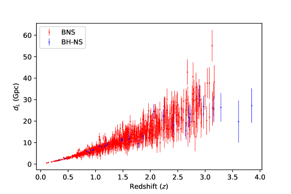
Figure 1: Mock GW catalogue of 1000 BNS merger events and 30 BH-NS merger events as standard sirens.

Abernathy et al. (2011) predicted event rates in ET. It is expected to observe $\mathcal{O}(10^{3}\sim 10^{7})$ BNS merger events and $\mathcal{O}(10^{3}\sim 10^{7})$ BH-NS events per year. However, this prediction is very uncertain. Li (2015) expected that only a small fraction ($\sim 10^{-3}$) of GW detections are accompanied by observed GRBs. Therefore we typically construct a catalogue of 1000 BNS events in our simulation. Besides, when the ratio between NS-BH and BNS events is assumed to be 0.03 as predicted by Advanced LIGO-Virgo network (Abadie et al., 2010; Li, 2015; Cai & Yang, 2017), 30 NS-BH events are included in the mock catalogue. These simulated events can reach out to a redshift $z\sim 4$. Figure 1 shows the $d_{L}$-$z$ diagram of our mock GW catalogue.

3 Calibration of GRB luminosity correlations

The GRB samples used for calibrating Amati relation ($E_{\text{iso}}$-$E_{\text{p}}$) and Ghirlanda relation ($E_{\gamma}$-$E_{\text{p}}$) are taken from Wang & Wang (2016) and Wang, Qi & Dai (2011) respectively.

The energy spectrum of GRBs is modeled by a broken power law (Band et al., 1993)

$$\Phi(E)=\begin{cases}(\frac{E}{100\text{ keV}})^{\alpha}\exp(-(2+\alpha)E/E_{\rm p,obs}),&E\leq\frac{\alpha-\beta}{2+\alpha}E_{\rm p,obs}\\ [\frac{(\alpha-\beta)E_{\text{p,obs}}/(2+\alpha)}{100\text{ keV}}]^{\alpha-\beta}\exp(\beta-\alpha)(\frac{E}{100\text{ keV}})^{\beta},&{\rm otherwise.}\end{cases}$$ (15)

where the typical spectral index values are taken to be $\alpha=-1.0$ and $\beta=-2.2$ if they are not given in the references.

For each GRB in the sample, the fluence $S$ have been corrected to 1-10000 keV energy band with $k$-correction (Bloom, Frail & Sari, 2001),

$$S_{\text{bolo}}=S\times\frac{\int_{1/(1+z)}^{10^{4}/(1+z)}E\Phi(E)\mathrm{d}E}{\int_{E_{\text{min}}}^{E_{\text{max}}}E\Phi(E)\mathrm{d}E},$$ (16)

where $E_{\text{min}}$ and $E_{\text{max}}$ are detection thresholds of the observing instrument. The isotropic energy $E_{\gamma,\text{iso}}$ and collimation-corrected energy $E_{\gamma}$ are

$$E_{\gamma,\text{iso}}=\frac{4\pi d_{L}^{2}S_{\text{bolo}}}{1+z},$$ (17)

and

$$E_{\gamma}=\frac{4\pi d_{L}^{2}S_{\text{bolo}}F_{\text{beam}}}{1+z}.$$ (18)

respectively, in which $F_{\text{beam}}=1-\cos\theta_{\text{jet}}$ is the beaming factor for jet opening angle $\theta_{\text{jet}}$. The luminosity distance $d_{L}$ of low-redshift GRBs is derived from GW standard sirens using linear interpolation method (Wang & Wang, 2016), which is independent of cosmology models

$$\ln d_{L}=\ln d^{\text{GW}}_{L,i}+\frac{z-z_{i}}{z_{i+1}-z_{i}}(\ln d^{\text{GW}}_{L,i}-\ln d^{\text{GW}}_{L,i}).$$ (19)

The $1\sigma$ error can be obtained by

$$\sigma_{\ln d_{L}}^{2}=\bigg{(}\frac{z_{i+1}-z}{z_{i+1}-z_{i}}\bigg{)}^{2}\epsilon_{\ln d^{\text{GW}}_{L,i}}^{2}+\bigg{(}\frac{z-z_{i}}{z_{i+1}-z_{i}}\bigg{)}^{2}\epsilon_{\ln d^{\text{GW}}_{L,i+1}}^{2},$$

where $\epsilon_{\ln d^{\text{GW}}_{L},i}\equiv\epsilon_{d^{\text{GW}}_{L,i}}/d^{\text{GW}}_{L,i}$ is the distance uncertainty of the $i$th GW event (the mock GW catalogue has been sorted by redshift before interpolation).

3.1 The $E_{\text{iso}}$-$E_{\text{p}}$ correlation

We parameterize the Amati relation ($E_{\text{iso}}$-$E_{\text{p}}$ correlation) (Amati et al., 2002) as

$$\log_{10}\frac{E_{\gamma,\text{iso}}}{1\text{ erg}}=a+b\log_{10}\bigg{[}\frac{E_{\text{p,obs}}(1+z)}{300\text{ keV}}\bigg{]},$$ (20)

where $E_{\text{p,obs}}(1+z)$ is the cosmological rest-frame spectral peak energy of GRB. The Markov chain Monte Carlo (MCMC) algorithm is applied to constrain intercept $a$, slope $b$ and intrinsic scatter $\sigma_{\text{int}}$ of the correlation. We use the python module $\mathtt{emcee}$ to carry out parameters fitting (Foreman-Mackey et al., 2013). The likelihood to fit the linear relation $y=ax+b$ (D’Agostini, 2005) is

$$L=\prod_{i=1}^{N}\frac{1}{\sqrt{2\pi}\sqrt{\sigma_{\text{int}}^{2}+\sigma^{2}_{y_{i}}+b^{2}\sigma^{2}_{x_{i}}}}\exp\bigg{[}\frac{-(y_{i}-a-bx_{i})^{2}}{2(\sigma_{\text{int}}^{2}+\sigma^{2}_{y_{i}}+b^{2}\sigma^{2}_{x_{i}})}\bigg{]}.$$ (21)

where $x\equiv\log_{10}[\frac{E_{\text{p,obs}}(1+z)}{300\text{ keV}}]$, $y\equiv\log_{10}\frac{E_{\gamma,\text{iso}}}{1\text{ erg}}$ and the propagated uncertainties of $y$ is calculated from

$$\sigma^{2}_{y}=\frac{\sigma^{2}_{S_{\text{bolo}}}}{(\ln 10\,\,S_{\text{bolo}})^{2}}.$$ (22)

3.2 The $E_{\gamma}$-$E_{\text{p}}$ correlation

The parametrization of the Ghirlanda relation ($E_{\gamma}$-$E_{\text{p}}$ correlation) (Ghirlanda, Ghisellini & Lazzati, 2004) is

$$\log_{10}\frac{E_{\gamma}}{1\text{ erg}}=a+b\log_{10}\bigg{[}\frac{E_{\text{p,obs}}(1+z)}{300\text{ keV}}\bigg{]}.$$ (23)

The likelihood function has the same form as $E_{\text{iso}}$-$E_{\text{p}}$ correlation’s, while the propagated uncertainties of $y\equiv\log_{10}\frac{E_{\gamma}}{1\text{ erg}}$ is calculated from

$$\sigma^{2}_{y}=\frac{\sigma^{2}_{S_{\text{bolo}}}F^{2}_{\text{beam}}+(S_{\text{bolo}})^{2}\sigma^{2}_{F_{\text{beam}}}}{(\ln 10\,\,S_{\text{bolo}}F_{\text{beam}})^{2}}.$$ (24)

The same procedure as handling $E_{\text{iso}}$-$E_{\text{p}}$ correlation is used to calibrate the $E_{\text{iso}}$-$E_{\text{p}}$ correlation.

3.3 Results

With our mock GW catalogue, the constraints on intercept $a$ and slope $b$ of Amati relation is $a=52.93\pm 0.04,b=1.41\pm 0.07$, $\sigma_{\text{int}}=0.39\pm 0.03$ ($1\sigma$) , while for Ghirlanda relation, $a=50.63\pm 0.08,b=1.50\pm 0.12$ and $\sigma_{\text{int}}=0.16\pm 0.04$ ($1\sigma$). The 1$\sigma$, 2$\sigma$ and 3$\sigma$ confidence contours and marginalized likelihood distributions are shown in Figure 2 and Figure 3 respectively. Wang & Wang (2016) standardized Amati relation of form $\log_{10}(E_{\gamma,\text{iso}}/\text{ erg})=a+b\log_{10}[E_{\text{p,obs}}(1+z)/\text{ keV}]$ with SNe Ia Union2.1 sample. Their fitting results are $a=48.46\pm 0.033$, $b=1.766\pm 0.007$ with $\sigma_{\text{ext}}=0.34\pm 0.04$. Amati et al. (2018) calibrated Amati relation of form $\log_{10}(E_{\text{p}}/\text{ keV})=q+m[\log_{10}(E_{\text{iso}}^{\text{cal}}/\text{ erg})-52]$, finding $q=2.06\pm 0.03$, $m=0.50\pm 0.12$ and $\sigma_{\text{int}}=0.20\pm 0.01$.

The calibrated GRB Hubble diagram is shown in Figure 4. The solid line in this figure is plotted based on the Planck15 cosmological parameters (Planck collaboration, 2016).

3.4 Constraining $\Lambda$CDM model and cosmological applications

We combine the calibrated GRB data and SNe Ia from Pantheon sample (Scolnic et al., 2018) to constrain non-flat $\Lambda$CDM model. The nuisance parameters {$\alpha$, $\beta$, $M_{B}^{1}$, $\Delta_{M}$} of SNe Ia lightcurve are fitted with cosmological parameters {$\Omega_{\text{m}}$, $\Omega_{\Lambda}$} simultaneously with the following total likelihood function

$$L\propto L_{\text{GRB}}\cdot L_{\text{SN}},$$

The likelihood function of GRB is given by

$$L_{\text{GRB}}=\prod_{i=1}^{N}\frac{1}{\sqrt{2\pi}\sigma_{\mu_{\text{GRB},i}}}\exp\bigg{[}\frac{-(\mu_{\text{th},i}-\mu_{\text{GRB},i})^{2}}{2\sigma_{\mu_{\text{GRB},i}}^{2}}\bigg{]}.$$ (25)

where the distance modulus uncertainty $\sigma_{\mu_{\text{GRB}}}$ is

$$\sigma_{\mu_{\text{GRB}}}^{2}=\bigg{(}\frac{5}{2}\sigma_{\log_{10}E_{\gamma,\text{iso}}}\bigg{)}^{2}+\bigg{(}\frac{5}{2\ln 10}\frac{\sigma_{S_{\text{bolo}}}}{S_{\text{bolo}}}\bigg{)}^{2}$$ (26)

and

$$\sigma_{\log_{10}E_{\gamma,\text{iso}}}^{2}=\sigma_{a}^{2}+\bigg{(}\sigma_{b}\log_{10}\frac{E_{\text{p,obs}}(1+z)}{300\text{ keV}}\bigg{)}^{2}+\bigg{(}\frac{b}{\ln 10}\frac{\sigma_{E_{\text{p,obs}}}}{E_{\text{p,obs}}}\bigg{)}^{2}+\sigma_{\text{int}}^{2}$$ (27)

The Hubble constant $H_{0}$ in our fitting is fixed to Planck15 (Planck collaboration, 2016) value. With the combined sample (GRBs + SNe), the best-fit values for non-flat $\Lambda$CDM model are $\Omega_{\text{m}}=0.33\pm 0.04$ and $\Omega_{\Lambda}=0.52\pm 0.08$ with 1$\sigma$ uncertainties. The constraints on $\Omega_{\text{m}}$, $\Omega_{\Lambda}$ and SNe Ia lightcurve parameters {$\alpha$, $\beta$, $M_{B}^{1}$, $\Delta_{M}$} are shown in Figure 5.

4 Summary

In this paper, we propose to calibrate the GRB luminosity relations using GW standard sirens. This method is model-independent and will overcome the circularity problem. The constraints for intercepts and slopes of Amati relation and Ghirlanda relation are $a=52.93\pm 0.04,b=1.41\pm 0.07$, $\sigma_{\text{int}}=0.39\pm 0.03$ ($1\sigma$) and $a=50.63\pm 0.08,b=1.50\pm 0.12$, $\sigma_{\text{int}}=0.16\pm 0.04$ ($1\sigma$) respectively with our mock GW catalogue. The performance of our method will improve with the upgrade of GW detector’s sensitivity, especially with third generation detectors ET (Abernathy et al., 2011), BBO (Cutler & Holz, 2009) and DECIGO (Kawamura et al., 2011). GRBs serve as a complementary tool to other cosmological probes such as SNe Ia, BAO and CMB. Besides, it plays a crucial role in constraining $w(z)$ especially at high redshifts (Wang, Qi & Dai, 2011), which may help us understanding the nature of dark energy.

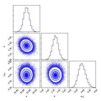
Figure 2: Confidence contours (1$\sigma$, 2$\sigma$ and 3$\sigma$) and marginalized likelihood distributions for intercept $a$ and slope $b$ in Amati relation.

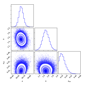
Figure 3: Confidence contours (1$\sigma$, 2$\sigma$ and 3$\sigma$) and marginalized likelihood distributions for intercept $a$ and slope $b$ in Ghirlanda relation.

Figure 4: Distance modulus of calibrated GRBs in comparison to Planck15 (Planck collaboration, 2016) $\Lambda$CDM cosmology (depicted in solid orange line).

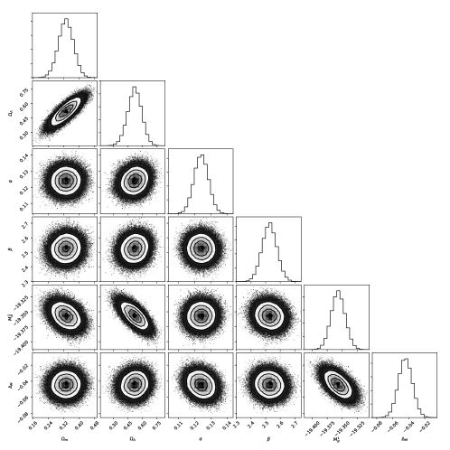
Figure 5: 1$\sigma$, 2$\sigma$ and 3$\sigma$ constraints on $\Omega_{\text{m}}$, $\Omega_{\Lambda}$ and SNe Ia lightcurve parameters {$\alpha$, $\beta$, $M_{B}^{1}$, $\Delta_{M}$} from ”calibrated” GRB and Pantheon SNe Ia sample.

References

- Planck collaboration (2016) Ade, P. A. R., et al. (Planck collaboration), 2016, A&A, 594, A13
- Abadie et al. (2010) Abadie, J., et al. (LIGO Scientific Collaboration), 2010, Nucl. Instrum. Methods Phys. Res., Sect. A, 624, 223 (2010)
- Abbott et al. (2017) Abbott, B. P., et al. (LIGO Scientific Collaboration and Virgo Collaboration), 2017, Phys. Rev. Lett., 119, 161101
- Abernathy et al. (2011) Abernathy, M., et al., 2011, Einstein gravitational wave telescope: conceptual design study, European Gravitational Observatory, Document No. ET-0106C-10
- Amati et al. (2002) Amati, L., et al., 2002, A&A390, 81.
- Amati (2006) Amati, L. 2006, MNRAS, 372, 233–245
- Amati et al. (2018) Amati, L., et al. arXiv:1811.08934v1
- Arun et al. (2005) Arun, K. G., , Iyer, B. R., Sathyaprakash, B. S., & Sundararajan, P. A. 2005, Phys. Rev. D, 71, 084008
- Avgoustidis, Verdec & Jimenez (2009) Avgoustidis, A., Verdec, L., & Jimenez, R. 2009, J. Cosmology Astropart. Phys, 06, 012
- Band et al. (1993) Band, D., et al. 1993, ApJ, 413, 281
- Barkana & Loeb (2004) Barkana, R., & Loeb, A. 2004, ApJ, 601, 64
- Berger (2007) Berger, E. 2007, ApJ, 670, 1254
- Blanchet et al. (2002) Blanchet, L., Faye, G., Iyer, B. R., & Joguet, B. 2002, Phys. Rev. D, 65, 061501
- Bloom, Frail & Sari (2001) Bloom, J. S., Frail, D. A., & Sari, R. 2001, AJ, 121, 2879
- Bromm, Coppi & Larson (2002) Bromm, V., Coppi, P. S., & Larson, R. B. 2002. ApJ, 564, 23
- Cai & Yang (2017) Cai, R. G., & Yang, T. 2017, Phys. Rev. D, 95, 044024
- Cucchiara et al. (2011) Cucchiara, A., et al. 2011, ApJ, 736, 7
- Cutler & Holz (2009) Cutler, C., & Holz, D. E. 2009, Phys. Rev. D, 80, 104009
- D’Agostini (2005) G. D’Agostini, G. 2005, arXiv:physics/0511182v1
- Dai, Liang & Xu (2004) Dai, Z. G., Liang, E. W., & Xu, D. 2004, ApJ, 612, L101
- Dainotti, Cardone & Capozziello (2008) Dainotti, M.G., Cardone, V.F., Capozziello, S., 2008, MNRAS, 391, L79
- Dainotti & Del Vecchio (2017) Dainotti, M. G., & Del Vecchio, R. 2017, New Astronomy Reviews, 77, 23
- Dainotti (2011) Dainotti, M. G., Ostrowski, M., & Willingale, R. 2011, MNRAS, 418, 2202
- Dainotti, Del Vecchio & Tarnopolski (2018) Dainotti, M. G., Del Vecchio, R., & Tarnopolski, . 2018, Advances in Astronomy, 4969503
- Dainotti & Amati (2018) Dainotti, M. G., & Amati, L. 2018, PASP, 130, 051001
- Foreman-Mackey et al. (2013) Foreman-Mackey, D., et al. 2013, PASP, 125, 306
- Fryer & Kalogera (2001) Fryer, C. L., & Kalogera, V. 2001, ApJ, 554, 548
- Ghirlanda, Ghisellini & Lazzati (2004) Ghirlanda, G., Ghisellini, G., & Lazzati, D. 2004, ApJ, 616, 331
- Ghirlanda et al. (2004) Ghirlanda, G., et al. 2004, ApJ, 613, L13
- Ghirlanda et al. (2006) Ghirlanda, G., et al. 2006, A&A, 452, 839
- Ghisellini et al. (2009) Ghisellini, G., et al. 2009, MNRAS, 393, 253
- Hartoog et al. (2015) Hartoog, O. E. et al., 2015, A&A, 580, A139
- Holz (1998) Holz, D. E. 1998, ApJ, 506, L1
- Hu, Yu & Wang (2017) Hu, J., Yu, H., & Wang, F. Y. 2017, ApJ, 836, 107
- Hui & Greene (2006) Hui, L., & Greene, P. B. 2006, Phys. Rev. D, 73, 123526
- Kawamura et al. (2011) Kawamura, S., et al. 2011, Class. Quantum Grav. 28, 094011
- Kodama et al. (2008) Kodama, Y., et al. 2008, MNRAS, 391, L1.
- Kumar & Zhang (2015) Kumar, P., & Zhang, B. 2015, Phys. Rep., 561, 1
- Li et al. (2008) Li, H., et al. 2008, ApJ, 680, 92
- Li (2015) Li, T. G. F., Extracting Physics from Gravitational Waves (Springer Theses, New York, 2015)
- Liang & Zhang (2005) Liang, E. W., & Zhang, B. 2005, ApJ, 633, 611
- Liang & Zhang (2006) Liang, E.W., & Zhang, B. 2006. MNRAS, 369, L37
- Liang, Zhang & Zhang (2007) Liang, E. W., Zhang, B. B., & Zhang, B. 2007, ApJ, 670, 565
- Liang et al. (2008) Liang, N., Xiao, W. K., Liu, Y., & Zhang, S. N. 2008, ApJ, 685, 354
- Liang et al. (2015) Liang, E. W., et al. 2015, ApJ, 813, 116
- Norris, Marani & Bonnell (2000) Norris, J. P., Marani, G. F., Bonnell, J. T. 2000, ApJ, 534, 248
- Oates et al. (2012) Oates, S. R., et al. 2012, MNRAS, 426, L86
- Rodney et al. (2015) Rodney, S. A., et al. 2015, AJ, 150, 156
- Sathyaprakash, Schutz & Van Den Broeck (2010) Sathyaprakash, B. S., B F Schutz, B. F., & Van Den Broeck, C. 2010, Class. Quantum Grav. 27, 215006
- Schaefer (2007) Schaefer, B. E. 2007, ApJ, 660, 16
- Schneider et al. (2001) Schneider, R., et al. 2001, MNRAS, 324, 797
- Schutz (1986) Schutz, B. F. 1986, Nature (London) 323, 310
- Scolnic et al. (2018) Scolnic, D. M., et al. 2018, ApJ, 859, 101
- Totani (1997) Totani, T. 1997, ApJ, 486, L71
- Totani et al. (2006) Totani, T., et al. 2006, PASJ, 58, 485
- Wang, Dai & Zhu (2007) Wang, F. Y., Dai, Z. G., & Zhu, Z. H. 2007, ApJ, 667, 1
- Wang & Dai (2009) Wang, F. Y., & Dai, Z. G. 2009, MNRAS, 400, L10
- Wang & Dai (2011) Wang, F. Y., & Dai, Z. G. 2011, A&A, 536, A96
- Wang et al. (2012) Wang, F. Y., et al. 2012, ApJ, 760, 27
- Wang (2013) Wang, F. Y. 2013, A&A, 556, A90
- Wang, Dai & Liang (2015) Wang, F. Y., Dai, Z. G., & Liang, E. W. 2015, New Astronomy Reviews, 67, 1
- Wang, Qi & Dai (2011) Wang, F. Y., Qi, S., & Dai, Z. G. 2011, MNRAS, 415, 3423
- Wang & Wang (2016) Wang, J. S., Wang, F. Y., Cheng, K. S., & Dai, Z. G. 2016, A&A, 585, A68
- Wang (2008) Wang, Y. 2008, Phys. Rev. D, 78, 123532
- Wei & Gao (2003) Wei, D. M., & Gao, W. H. 2003, MNRAS, 345, 743
- Yonetoku et al. (2004) Yonetoku, D., et al. 2004, ApJ, 609, 935
- Zhao et al. (2011) Zhao, W., Van Den Broeck, C., Baskaran, D., & Li, T. G. F. 2011, Phys. Rev. D, 83, 023005
- Zhao & Wen (2018) Zhao, W., & Wen, L. Q. 2018, Phys. Rev. D, 97, 064031