Microlocal Analysis of a Compton Tomography Problem

Abstract

Here we present a novel microlocal analysis of a new toric section transform which describes a two dimensional image reconstruction problem in Compton scattering tomography and airport baggage screening. By an analysis of two separate limited data problems for the circle transform and using microlocal analysis, we show that the canonical relation of the toric section transform is 2–1. This implies that there are image artefacts in the filtered backprojection reconstruction. We provide explicit expressions for the expected artefacts and demonstrate these by simulations. In addition, we prove injectivity of the forward operator for $L^{\infty}$ functions supported inside the open unit ball. We present reconstructions from simulated data using a discrete approach and several regularizers with varying levels of added pseudo-random noise.

44A12, 35S30, 65R32, 94A08

1 Introduction

We consider the Compton scattering tomography acquisition geometry displayed in figure 2, which illustrates an idealized source–detector geometry in airport baggage screening representing the Real Time Tomography (RTT) geometry [27]. See appendix A for more detail on the potential for the application of this work in airport baggage screening. The inner circle (of smaller radius) represents a ring of fixed energy sensitive detectors and the outer circle a ring of fixed, switched X-ray sources, which we will assume for the purposes of this paper can be simulated to be monochromatic (e.g. by varying the X-ray tube voltage and taking finite differences in energy or by source filtering [10, 11]). It is noted that the RTT geometry is three dimensional [27], but we assume a two dimensional scattering geometry as done in [29]. Further we note that in the desired application in airport baggage screening we expect the data to be very noisy. Later in section 4 we simulate the noisy data using an additive Gaussian model with a significant level (up to $5\%$) and show that we can combat the noise effectively using the methods of [5] (specifically the “IRhtv” method).

Compton scattering describes the inelastic scattering process of a photon with charged particles (usually electrons). The energy loss is given by the equation

(1) $$E^{\prime}=\frac{E}{1+(E/E_{0})(1-\cos\omega)},$$

Figure 1: Part of a toric section $T=C_{1}\cup C_{2}$ with points of self-intersection at source and detector points $\mathbf{s}$ and $\mathbf{d}$ respectively. The incoming photons (illustrated by wavy lines) have initial energy $E$ and scatter at a fixed angle $\omega<\pi/2$ along scattering sites $\mathbf{x}\in T$. The resulting (scattered) photon energy is $E^{\prime}$ as in equation (1). The electron density $f$ (the red rectangle) is supported within the green circle (the unit ball, see figure 2).

where $E^{\prime}$ is the scattered energy, $E$ is the initial energy, $\omega$ is the scattering angle and $E_{0}$ denotes the electron rest energy. If the source is monochromatic ($E$ is fixed) and we can measure the scattered energy $E^{\prime}$, then the scattering angle $\omega$ of the interaction is determined by equation (1). This implies that the locus of Compton scatterers in the plane is a toric section $T=C_{1}\cup C_{2}$ (the union of two intersecting circular arcs). See figure 1. Hence we model the scattered intensity collected at the detector $\mathbf{d}$ with scattering angle $\omega$ (determined by the scattering energy $E^{\prime}$ in (1) and which determines the radius $r$ of the circular arcs in figure 2) as integrals of the electron charge density $f$ (represented by a real valued function) over toric sections $T$. This is the idea behind two dimensional Compton scattering tomography [18, 20, 21, 29]. Note that the larger circular arcs of figure 2 (which make up the majority of the circle circumference) do not intersect the scanning region, and hence we can consider integrals over whole toric sections (not just the part of $T$ depicted in figure 1). In three dimensions, the surface of scatterers is described by the surface of revolution of a toric section about its central axis, namely a spindle torus. In [30, 31] the inversion and microlocal aspects of a spindle torus integral transform are considered. In [24] Rigaud considers a related Compton model with attenuation, and Rigaud and Hahn develop and analyze a clever contour reconstruction method for a 3-d model [25].

The set of toric sections whose tips (the points of intersection of $C_{1}$ and $C_{2}$) lie on two circles (as in figure 2) is three dimensional. Indeed we can vary a source and detector coordinate on $S^{1}\times S^{1}$ and the radius of the circles $r$. In this paper we consider the two dimensional subset of toric sections whose central axis (the line through the points of intersection of $C_{1}$ and $C_{2}$) intersects the origin. This can be parametrized by a rotation about the origin ($\theta\in S^{1}$) and the radius $r\geq 2$, as we shall see later in section 3.

In [29] the RTT geometry is considered and the scattered intensity is approximated as a set of integrals over discs whose boundaries intersect a given source point, and inversion techniques and stability estimates are derived through an equivalence with the Radon transform. Here we present a novel toric section transform (which describes the scattered intensity exactly) and analyse its stability from a microlocal standpoint. So far the results of Natterer [17] have been used to derive Sobolev space estimates for the disc transform presented in [29], but the microlocal aspects of the RTT geometry in Compton tomography are less well-studied. We aim to address this here. We explain the expected artefacts in a reconstruction from toric section integral data through an analysis of the canonical relation of a toric section transform, and injectivity results are provided for $L^{\infty}$ functions inside the unit ball. The expected artefacts are shown by simulations and are as predicted by the theory. We also give reconstructions of two simulated test phantoms with varying levels of added pseudo-random noise. In [31] it is suggested to use a Total Variation (TV) regularization technique to combat the artefacts in a three dimensional Compton tomography problem. Here we show that we can combat the non-local artefacts (due to the 2-1 nature of the canonical relation) present in the reconstruction effectively in two dimensions using a discrete approach and a heuristic TV regularizer.

Figure 2: Part of a toric section $T=C_{1}\cup C_{2}$ with axis of rotation $\theta=(0,1)$, tube center offset $s=\sqrt{r^{2}-4}$ and tube radius $r$. Here $\cos\omega=\frac{\sqrt{r^{2}-4}}{r}$. The coordinates $\mathbf{c}_{1}$ and $\mathbf{c}_{2}$ denote the centers of the circles which the arcs $C_{1}$ and $C_{2}$ lie on respectively. The detector ring (green circle, radius 1, center $O$) is the scanning region, where the density $f$ (the red square) is supported. The source ring is the blue circle, which has radius 3 and center $O$.

In section 2 we recall some definitions and results on Fourier Integral Operators (FIO’s) and microlocal analysis before introducing a new toric section transform in section 3, which describes the Compton scattered intensity collected by the acquisition geometry in figure 2. Later in section 3.1 we provide a novel microlocal analysis of the toric section transform when considered as an FIO. Through an analysis of the canonical relations of two circle transforms separately (whose sum is equivalent to the toric section transform), we show that the canonical relation of the toric section transform is 2–1 and provide explicit expressions for the artefacts expected in a reconstruction from toric section integral data.

In section 3.2 we prove the injectivity of the toric section transform on the set of $L^{\infty}$ functions in the unit ball. This uses a similar parameterization of circular arcs to Nguyen and Truong in [18] and proves the injectivity by a decomposition into the Fourier series components and using the ideas of Cormack [2].

In section 4, we present a practical reconstruction algorithm for the recovery of two dimensional densities from toric section integral data and provide simulated reconstructions of two test phantoms (one simple and one complex) with varying level of added pseudo-random noise. Here we use a discrete approach. That is we discretize the toric section integral operator (stored as a sparse matrix) on a pixel grid (assuming a piecewise constant density) and use an iterative technique (e.g. a conjugate gradient method) to solve the sparse set of linear equations described by the discretized operator with regularization (e.g. Tikhonov or total variation). We demonstrate the non-local artefacts in the reconstruction by an application of the discretized normal operator ($A^{T}A$, where $A$ is the discrete from of the toric section transform) to a delta function, and show that the artefacts are exactly as predicted by the theory presented in section 3.1 by a side by side comparison. We further show that we can effectively combat the non-local reconstruction artefacts by applying the “IRhtv” method of [5] (see also [9]).

2 Microlocal definitions

We now provide some definitions.

Definition 2.1 ([14, Definition 7.1.1]).

For a function $f$ in the Schwartz space $S(\mathbb{R}^{n})$ we define the Fourier transform and its inverse as

(2) $$\begin{split}\mathcal{F}f(\xi)&=\int_{\mathbb{R}^{n}}e^{-ix\cdot\xi}f(x)\mathrm{d}x,\\ \mathcal{F}^{-1}f(x)&=(2\pi)^{-n}\int_{\mathbb{R}^{n}}e^{ix\cdot\xi}f(\xi)\mathrm{d}\xi.\end{split}$$

We use the standard multi-index notation; let $\alpha=(\alpha_{1},\alpha_{2},\dots,\alpha_{n})\in\left\{0,1,2,\dots\right\}^{n}$ be a multi-index and $f$ a function on ${{\mathbb{R}}^{n}}$, then $\partial^{\alpha}f=\left(\frac{\partial}{\partial x_{1}}\right)^{\alpha_{1}}\left(\frac{\partial}{\partial x_{2}}\right)^{\alpha_{2}}\cdots\left(\frac{\partial}{\partial x_{n}}\right)^{\alpha_{n}}f$.

We identify cotangent spaces on Euclidean spaces with the underlying Euclidean spaces so if $X$ is an open subset of ${{\mathbb{R}}^{n}}$ and $(x,\xi)\in X\times{{\mathbb{R}}}^{N}$ then $T^{*}_{(x,\xi)}\left(X\times{{\mathbb{R}}}^{N}\right)$ is identified with ${{\mathbb{R}}^{n}}\times{{\mathbb{R}}}^{N}$. Under this identification, if $\phi=\phi(x,\xi)$ for $(x,\xi)\in X\times{{\mathbb{R}}}^{N}$ then

$$\begin{gathered}\mathrm{d}_{x}\phi=\left(\frac{\partial\phi}{\partial x_{1}},\frac{\partial\phi}{\partial x_{2}},\cdots,\frac{\partial\phi}{\partial x_{n}}\right),\ \mathrm{d}_{\xi}\phi=\left(\frac{\partial\phi}{\partial\xi_{1}},\frac{\partial\phi}{\partial\xi_{2}},\cdots,\frac{\partial\phi}{\partial\xi_{N}}\right)\\ \text{ and }\ \mathrm{d}\phi(x,\xi)=\left(\mathrm{d}_{x}\phi(x,\xi),\mathrm{d}_{\xi}\phi(x,\xi)\right)\in{{\mathbb{R}}^{n}}\times{{\mathbb{R}}}^{N}.\end{gathered}$$

Definition 2.2 ([14, Definition 7.8.1]).

Let $X$ be an open subset of ${{\mathbb{R}}^{n}}$ and let $m\in\mathbb{R}$. Then we define $S^{m}(X\times\mathbb{R}^{N})$ to be the set of $a\in C^{\infty}(X\times\mathbb{R}^{N})$ such that for every compact set $K\subset X$ and all multi–indices $\alpha,\beta$ the bound

$$\left|\partial^{\beta}_{x}\partial^{\alpha}_{\xi}a(x,\xi)\right|\leq C_{\alpha,\beta,K}(1+|\xi|)^{m-|\alpha|},\ \ \ x\in K,\ \xi\in\mathbb{R}^{n},$$

holds for some constant $C_{K}$. The elements of $S^{m}$ are called symbols of order $m$.

Note that these symbols are sometimes denoted $S^{m}_{1,0}$

Definition 2.3 ([15, Definition 21.2.15]).

A function $\phi=\phi(x,\xi)\in C^{\infty}(X\times\mathbb{R}^{N}\backslash 0)$ is a phase function if $\phi(x,\lambda\xi)=\lambda\phi(x,\xi)$, $\forall\lambda>0$ and $\mathrm{d}\phi$ is nowhere zero. A phase function is clean if the critical set $\Sigma_{\phi}=\{(x,\xi)\ :\ \mathrm{d}_{\xi}\phi(x,\xi)=0\}$ is a smooth manifold with tangent space defined by $\mathrm{d}\left(\mathrm{d}_{\xi}\phi\right)=0$.

By the implicit function theorem the requirement for a phase function to be clean is satisfied if $\mathrm{d}\left(\mathrm{d}_{\xi}\phi\right)$ has constant rank.

Definition 2.4 ([15, Definition 21.2.15] and [16, Section 25.2]).

Let $X\subset\mathbb{R}^{n_{x}}$, $Y\subset\mathbb{R}^{n_{y}}$ be open sets. Let $\phi\in C^{\infty}\left(X\times Y\times\left(\mathbb{R}^{N}\setminus 0\right)\right)$ be a clean phase function. Then, the critical set of $\phi$ is

$$\Sigma_{\phi}=\{(x,y,\xi)\in X\times Y\times\mathbb{R}^{N}\setminus\mathbf{0}:\mathrm{d}_{\xi}\phi=0\}.$$

The canonical relation parametrized by $\phi$ is defined as

(3) $$\mathcal{C}= \left\{\left((y,\mathrm{d}_{y}\phi(x,y,\xi)),(x,-\mathrm{d}_{x}\phi(x,y,\xi))\right):(x,y,\xi)\in\Sigma_{\phi}\right\},$$

Definition 2.5.

Let $X\subset\mathbb{R}^{n_{x}}$, $Y\subset\mathbb{R}^{n_{y}}$ be open sets. A Fourier integral operator (FIO) of order $m+N/2-(n_{x}+n_{y})/4$ is an operator $A:C^{\infty}_{0}(X)\to\mathcal{D}^{\prime}(Y)$ with Schwartz kernel given by an oscillatory integral of the form

(4) $$K_{A}(x,y)=\int_{\mathbb{R}^{N}}e^{i\phi(x,y,\xi)}a(x,y,\xi)\mathrm{d}\xi,$$

where $\phi$ is a clean phase function and $a\in S^{m}(X\times Y\times\mathbb{R}^{N})$ a symbol. The canonical relation of $A$ is the canonical relation of $\phi$ defined in (3).

This is a simplified version of the definition of FIO in [4, Section 2.4] or [16, Section 25.2] that is suitable for our purposes since our phase functions are global. For general information about FIOs see [4, 15, 16].

Definition 2.6.

Let $\mathcal{C}\in T^{*}(Y\times X)$ be the canonical relation associated to the FIO $A:\mathcal{E}^{\prime}(X)\to\mathcal{D}^{\prime}(Y)$. Then we denote $\pi_{L}$ and $\pi_{R}$ to be the natural left- and right-projections of $\mathcal{C}$, $\pi_{L}:\mathcal{C}\to T^{*}Y\backslash 0$ and $\pi_{R}:\mathcal{C}\to T^{*}X\backslash 0$.

We have the following result from [16].

Proposition 2.7.

Let $\dim(X)=\dim(Y)$. Then at any point in $\mathcal{C}$:

1. if one of $\pi_{L}$ or $\pi_{R}$ is a local diffeomorphism, then $\mathcal{C}$ is a local canonical graph;

2. if one of the projections $\pi_{R}$ or $\pi_{L}$ is singular at a point in $\mathcal{C}$, then so is the other. The type of the singularity may be different but both projections drop rank on the same set

   (5) $$\Sigma=\{(y,\eta;x,\xi)\in\mathcal{C}:\det(\mathrm{d}\pi_{L})=0\}=\{(y,\eta;x,\xi)\in\mathcal{C}:\det(\mathrm{d}\pi_{R})=0\}.$$

If a FIO $\mathcal{F}$ satisfies our next definition and $\mathcal{F}^{t}$ is its formal adjoint, then $\mathcal{F}^{t}\mathcal{F}$ (or $\mathcal{F}^{t}\phi\mathcal{F}$ where $\phi\in\mathcal{D}(Y)$ if $\mathcal{F}$ and $\mathcal{F}^{t}$ cannot be composed) is a pseudodifferential operator [7, 22].

Definition 2.8 (Semi-global Bolker Assumption).

Let $\mathcal{F}:\mathcal{E}^{\prime}(X)\to\mathcal{D}^{\prime}(Y)$ be a FIO with canonical relation $\mathcal{C}$ then $\mathcal{F}$ (or $\mathcal{C}$) satisfies the semi-global Bolker Assumption if the natural projection $\pi_{Y}:\mathcal{C}\to T^{*}(Y)$ is an injective immersion.

3 A toric section transform

In this section we recall some notation and definitions and introduce a toric section transform which models the intensity of scattered radiation described by the acquisition geometry in figure 2. This section contains our main theoretical results. We describe microlocally the expected artefacts in any backprojection reconstruction from toric section integral data (Theorem 3.6 and Remarks 3.8 and 3.10). In addition, we prove the injectivity of the toric section transform using integral equations techniques (Theorem 3.11 and Remark 3.13).

For $r>0$, let $B_{r}$ be the open disk centered at the origin of radius $r$ and let $B=B_{1}$ denote the open unit disk. For $X$ an open subset of $\mathbb{R}^{n}$, let $\mathcal{D}^{\prime}(X)$ denote the vector space of distributions on $X$, and let $\mathcal{E}^{\prime}(X)$ denote the vector space of distributions with compact support contained in $X$.

Let us parametrize points on the unit circle, $\theta\in S^{1}$ as $\theta=\theta(\alpha)=(\cos\alpha,\sin\alpha)$, for $\alpha\in[0,2\pi]$, and let $\theta_{\alpha}=\frac{d\theta}{d\alpha}$ be the unit vector $\pi/2$ radians counterclockwise (CCW) from $\theta$. When the choice of $\alpha$ is understood, then we will write $\theta$ for $\theta(\alpha)$.

Let $(r,\alpha)\in Y:=(2,\infty)\times[0,2\pi]$. To define the toric section, we first define two circular arcs and their centers. For $(r,\alpha)\in Y$ define

$$\begin{gathered}s=\sqrt{r^{2}-4},\quad\mathbf{c}_{1}=\mathbf{c}_{1}(r,\alpha)=\theta(\alpha)+s\theta_{\alpha}(\alpha),\quad\mathbf{c}_{2}=\mathbf{c}_{2}(r,\alpha)=\theta(\alpha)-s\theta_{\alpha}(\alpha)\\ C_{1}=C_{1}(r,\alpha)=\{\mathbf{x}\in\mathbb{R}^{2}:\mathbf{x}\cdot\theta_{\alpha}\leq 0,\ |\mathbf{x}-\mathbf{c}_{1}(r,\alpha)|^{2}-r^{2}=0\},\\ C_{2}=C_{2}(r,\alpha)=\{\mathbf{y}\in\mathbb{R}^{2}:\mathbf{y}\cdot\theta_{\alpha}\geq 0,\ |\mathbf{y}-\mathbf{c}_{2}(r,\alpha)|^{2}-r^{2}=0\}.\end{gathered}$$

When the choice of $(r,\alpha)$ is understood, we will refer to the arcs as $C_{j}$ and their centers as $\mathbf{c}_{j}$ for $j\in\left\{1,2\right\}$.

The toric transform integrates functions on $B$ over the toric sections, $C_{1}(r,\alpha)\cup C_{2}(r,\alpha)$: let $f\in C^{\infty}_{0}(B)$ represent the charge density in the plane. Then, we define the circle transforms

(6) $$\mathcal{T}_{1}f(r,\alpha)=\int_{C_{1}}f\mathrm{d}s,\ \ \ \ \ \ \ \ \mathcal{T}_{2}f(r,\alpha)=\int_{C_{2}}f\mathrm{d}s.$$

and the toric section transform

(7) $$\mathcal{T}f(r,\alpha)=\int_{C_{1}\cup C_{2}}f\mathrm{d}s=\mathcal{T}_{1}(f)(r,\alpha)+\mathcal{T}_{2}(f)(r,\alpha)$$

where $\mathrm{d}s$ denotes the arc element on a circle.

Remark 3.1.

Let $j=1,2$. The adjoint, $\mathcal{T}^{t}_{j}$, of $\mathcal{T}_{j}$ is defined on distributions by duality. For $g\in\mathcal{D}(Y)$ and $\mathbf{x}\in{{\mathbb{R}}^{2}}\setminus\mathbf{0}$, $\mathcal{T}^{t}g(\mathbf{x})$ is a weighted integral of $g$ over all toric sections through $\mathbf{x}$. Since there are no toric sections intersecting points outside of $B_{3}$, we assume $\mathbf{x}\in B_{3}$. We also note that no toric sections go through $\mathbf{0}$–toric sections close to $\mathbf{0}$ have values of $r\approx\infty$.

Furthermore, for fixed $\mathbf{x}\in B_{3}\setminus B$, the values of $\alpha$ such that $\mathbf{x}\in C_{j}(r,\alpha)$ (for some $r$) is a proper subinterval of $[0,2\pi]$.

Since the set of toric sections is unbounded, $\mathcal{T}^{t}$ must be defined on distributions of compact support.

To deal with all of these inconveniences, we define a modified adjoint. Let $\varphi:(2,\infty)\to{{\mathbb{R}}}$ be smooth and with compact support in $(2,M)$ for some $M>2$. One can also assume $0\leq\varphi\leq 1$ and $\varphi=1$ on most of $(2,M)$. We define the cutoff-adjoint $\mathcal{T}^{*}_{j}:\mathcal{D}^{\prime}(Y)\to\mathcal{D}^{\prime}(B_{3})$. For $g\in\mathcal{D}^{\prime}(Y)$,

(8) $$\mathcal{T}^{*}_{j}g=\mathcal{T}^{t}_{j}(\varphi g),\qquad\mathcal{T}^{*}=\mathcal{T}_{1}^{*}+\mathcal{T}_{2}^{*}.$$

Let $\rho_{\min}=M-\sqrt{M^{2}-3}$. Then, $\mathcal{T}^{*}g(\mathbf{x})=0$ for $\mathbf{x}\in B_{\rho_{\min}}\setminus\mathbf{0}$. This is true because $\rho_{\min}$ is the closest distance of the arcs $C_{1}(r,\alpha)$ and $C_{2}(r,\alpha)$ get to the origin for all $(r,\alpha)\in(2,M)\times[0,2\pi]$. Therefore, we define $\mathcal{T}^{*}g(0)=0$ and $\mathcal{T}^{*}g$ is smooth near $0$. This also means for $f\in\mathcal{E}^{\prime}(B_{3})$ that $\mathcal{T}^{*}\mathcal{T}f(\mathbf{x})=0$ if $\mathbf{x}\in B_{\rho_{\min}}$.

In this section, we will study the microlocal properties of $\mathcal{T}^{*}\mathcal{T}$. In Remark 3.8, we generalize our results to a more general filtered backprojection. The main results of this section are as follows. Let $f\in\mathcal{E}^{\prime}(B)$ have a singularity (e.g., region boundary) at $\mathbf{w}\in B$ in direction $\xi\in{{\mathbb{R}}^{n}}\setminus\mathbf{0}$, with $\mathbf{w}\cdot\xi\neq 0$, and let $\xi^{\prime}=\xi/|\xi|$. Our main theorem (Theorem 3.6) proves the existence of image artefacts corresponding to $(\mathbf{w},\xi)$ in a reconstruction from $\mathcal{T}f$ data at two points $\mathbf{x},\mathbf{y}\in\mathbb{R}^{2}$. The expression for $\mathbf{y}$ is given explicitly by

(9) $$\mathbf{y}=\nu[\theta_{\alpha},\theta]\begin{bmatrix}-\theta_{\alpha}^{T}\\ \frac{2}{s}\theta_{\alpha}^{T}-\theta^{T}\end{bmatrix}\mathbf{w},$$

where $r=\frac{|\mathbf{w}|^{2}+3}{2(\mathbf{w}\cdot\xi^{\prime})}$ and $\theta$ satisfies

$$\begin{pmatrix}1&s\\ -s&1\end{pmatrix}\theta=\mathbf{w}-r\xi^{\prime},$$

and $\nu>0$ is chosen so that $\mathbf{y}\in C_{2}$. The artefact at $\mathbf{y}$ comes about when the singularity at $(\mathbf{w},\xi)$ is (co)normal to a $C_{1}$ arc and is detected by $\mathcal{T}_{1}$ but backprojected by $\mathcal{T}_{2}^{*}$.

The expression for $\mathbf{x}$ is given by

$$\mathbf{x}=\frac{1}{\nu}[\theta_{\alpha},\theta]\begin{bmatrix}-\theta_{\alpha}^{T}\\ -\frac{2}{s}\theta_{\alpha}^{T}-\theta^{T}\end{bmatrix}\mathbf{w},$$

where $r=\frac{|\mathbf{w}|^{2}+3}{2(\mathbf{w}\cdot\xi^{\prime})}$ and $\theta$ satisfies

$$\begin{pmatrix}1&-s\\ s&1\end{pmatrix}\theta=\mathbf{w}-r\xi^{\prime},$$

and $\nu>0$ is chosen so that $\mathbf{x}\in C_{1}$. The artefact at $\mathbf{x}$ comes about when the singularity at $(\mathbf{w},\xi)$ is (co)normal to a $C_{2}$ arc and is detected by $\mathcal{T}_{2}$ but backprojected by $\mathcal{T}_{1}^{*}$.

A visualization of the predicted image artefacts when $f$ is a delta distribution is given in figure 3.

3.1 Microlocal Properties of $\mathcal{T}_{j}$ and $\mathcal{T}$

Since we do not consider the points of intersection of the arcs $C_{1}$ and $C_{2}$ (since distributions in the domain of $\mathcal{T}$, $\mathcal{E}^{\prime}(B)$, are supported away from them), we can consider the microlocal properties of the circle transforms $\mathcal{T}_{1}$ and $\mathcal{T}_{2}$ separately. Let $Y=[0,2\pi]\times(2,\infty)$. When considering functions and distributions on $Y$, we use the standard identification of $[0,2\pi]$ with the unit circle $S^{1}$, $\alpha\mapsto\theta(\alpha)=(\cos(\alpha),\sin(\alpha))$.

We first show $\mathcal{T}_{1}$ and $\mathcal{T}_{2}$ are FIO.

Proposition 3.2.

$\mathcal{T}_{1}$ and $\mathcal{T}_{2}$ are both FIO of order $-1/2$. Their canonical relations are

(10) $$\mathcal{C}_{1}=\Big{\{}\big{(} r,\alpha,-2\sigma\mathbf{x}\cdot(\theta_{\alpha}-s\theta),-\frac{2\sigma r}{s}(\mathbf{x}\cdot\theta_{\alpha});\mathbf{x},-2\sigma(\mathbf{x}-\mathbf{c}_{1}(r,\alpha))\big{)}:$$

$$\quad(r,\alpha)\in Y,\sigma\in\mathbb{R}\setminus\mathbf{0},\mathbf{x}\in C_{1}(r,\alpha)\cap B\Big{\}}.$$

$$\mathcal{C}_{2}=\Big{\{}\big{(} \alpha,r,-2\sigma\mathbf{y}\cdot(\theta_{\alpha}+s\theta),\frac{2\sigma r}{s}(\mathbf{y}\cdot\theta_{\alpha});\mathbf{y},-2\sigma(\mathbf{y}-\mathbf{c}_{2}(r,\alpha))\big{)}:$$

$$\quad(r,\alpha)\in Y,\sigma\in\mathbb{R}\backslash\{0\},\mathbf{y}\in C_{2}(r,\alpha)\cap B,\Big{\}}.$$

For $j=1,2$, we let $\widetilde{\mathcal{C}}_{j}$ be defined as $\mathcal{C}_{j}$ except that $\mathbf{x}$ or $\mathbf{y}$ is not restricted to be in $B$ and we let $\widetilde{\mathcal{C}}=\widetilde{\mathcal{C}}_{1}\cup\widetilde{\mathcal{C}}_{2}$.

Proof 3.3.

We briefly explain why $\mathcal{T}_{2}$ is a FIO and we calculate its canonical relation. Let $Z=\left\{(r,\alpha,\mathbf{y})\in Y\times B\hskip 0.85358pt:\hskip 0.85358pt|\mathbf{y}-\mathbf{c}_{2}(r,\alpha)|^{2}-r^{2}=0\right\}$. From calculations in [7, 22] the Schwartz kernel of $\mathcal{T}_{2}$ is integration over $Z$ and so the this Schwartz kernel is a Fourier integral distribution with phase function $\phi_{2}(\mathbf{y},r,\alpha,\sigma)=\sigma\left(|\mathbf{y}-\mathbf{c}_{2}(r,\alpha)|^{2}-r^{2}\right)$. This is true because, for functions supported in $B$, $\mathcal{T}_{2}$ can be viewed as integrating on the full circle defined by $|\mathbf{y}-\mathbf{c}_{2}(r,\alpha)|^{2}-r^{2}=0$.

Using Definition 2.4 one sees that the canonical relation of $\mathcal{T}_{2}$ is given by the expression in (10). One can easily check that the projections $\pi_{L}(\mathcal{C}_{2})$ and $\pi_{R}(\mathcal{C}_{2})$ do not map to the zero section so $\mathcal{T}_{2}:\mathcal{E}^{\prime}(B)\to\mathcal{D}^{\prime}(Y)$ [13].

The operator $\mathcal{T}_{2}$ is a Radon transform and therefore its symbol is of order zero (see, e.g., [22]), so one can use the order calculation in Definition 2.5 to show that the order of $\mathcal{T}_{2}$ is $-1/2$.

In a similar way, one shows that $\mathcal{T}_{1}$ is an FIO with phase function $\phi_{1}(\mathbf{x},r,\alpha,\sigma)=\sigma\left(|\mathbf{x}-\mathbf{c}_{1}(r,\alpha)|^{2}-r^{2}\right)$.

We now prove that each $\mathcal{T}_{j}$ satisfies the Bolker Assumption.

Theorem 3.4.

For $j=1,2$, the left projection $\pi_{L}:\widetilde{\mathcal{C}}_{j}\to T^{*}(Y)$ is an injective immersion. Therefore, $\pi_{L}:\mathcal{C}_{j}\to T^{*}(Y)$ is an injective immersion and so $\mathcal{T}_{j}$ satisfies the semi-global Bolker Assumption (Definition 2.8).

The operators $\mathcal{T}_{i}^{*}$ and $\mathcal{T}_{j}$ can be composed as FIO and the compositions all have order $-1$.

Proof 3.5.

We will prove this theorem for $\mathcal{T}_{2}$ and the proof for $\mathcal{T}_{1}$ is completely analogous. We first show that $\pi_{L}$ is an immersion.

As noted above, if $\alpha$ is known, then we let $\theta=\theta(\alpha)$ and $\theta_{\alpha}=(-\sin\alpha,\cos\alpha)$. For bookkeeping reasons, if $\beta\in[0,2\pi]$, the vector in $S^{1}$ corresponding to $\beta$ will be denoted $\psi=(\cos\beta,\sin\beta)$ and we let $\psi_{\beta}=(-\sin\beta,\cos\beta)$ be the unit vector $\pi/2$ radians CCW from $\psi$. This allows us to parametrize points on $C_{2}(r,\alpha)$ by

(11) $$\mathbf{y}=\mathbf{y}(r,\alpha,\beta)=\mathbf{c}_{2}+r\psi=\mathbf{c}_{2}(r,\alpha)+r(\cos\beta,\sin\beta),$$

for $\beta$ in an open interval containing $[0,2\pi]$. Then,

(12) $$(r,\alpha,\beta,\sigma)\mapsto\lambda_{2}(r,\alpha,\beta,\sigma):=\left(r,\alpha,\sigma\mathrm{d}_{\alpha}\phi_{2},\sigma\mathrm{d}_{r}\phi_{2};\mathbf{y}(r,\alpha,\beta),-\sigma\mathrm{d}_{\mathbf{y}}\phi_{2}\right)\in\mathcal{C}_{2}$$

gives coordinates on the canonical relation $\mathcal{C}_{2}$. Using these coordinates and after simplification, the map $\pi_{L}$ is given by

(13) $$\pi_{L}(\lambda(r,\alpha,\beta,\sigma))=\left(r,\alpha,-2\sigma r\psi\cdot(\theta_{\alpha}+s\theta),\frac{2\sigma r}{s}(-s+r\psi\cdot\theta_{\alpha})\right)$$

and

(14) $$D\pi_{L}=\begin{pmatrix}1&0&0&0\\ 0&1&0&0\\ a_{3,1}&a_{3,2}&-2\sigma r\psi_{\beta}\cdot(\theta_{\alpha}+s\theta)&-2r\psi\cdot(\theta_{\alpha}+s\theta)\\ a_{4,1}&a_{4,2}\par&\frac{2\sigma r^{2}}{s}(\psi_{\beta}\cdot\theta_{\alpha})\par&\frac{2r^{2}}{s}\left(-\frac{s}{r}+\psi\cdot\theta_{\alpha}\right)\end{pmatrix}.$$

It follows that

(15) $$\begin{split}\det D\pi_{L}&=-\frac{4r^{3}\sigma}{s}\det\begin{pmatrix}\psi_{\beta}\cdot(\theta_{\alpha}+s\theta)&\psi\cdot(\theta_{\alpha}+s\theta)\\ \psi_{\beta}\cdot\theta_{\alpha}&-\frac{s}{r}+\psi\cdot\theta_{\alpha}\end{pmatrix}\\ &=-\frac{4r^{3}\sigma}{s}\left(-\frac{s}{r}\psi_{\beta}\cdot(\theta_{\alpha}+s\theta)+(\psi\cdot\theta_{\alpha})(\psi_{\beta}\cdot\theta_{\alpha}+s\psi_{\beta}\cdot\theta)-(\psi_{\beta}\cdot\theta_{\alpha})(\psi\cdot\theta_{\alpha}+s\psi\cdot\theta)\right)\\ &=-4r^{3}\sigma\left(-\frac{1}{r}\psi_{\beta}\cdot(\theta_{\alpha}+s\theta)+(\psi\cdot\theta_{\alpha})(\psi_{\beta}\cdot\theta)-(\psi_{\beta}\cdot\theta_{\alpha})(\psi\cdot\theta)\right)\\ &=4r^{3}\sigma\left(\frac{1}{r}(\psi\cdot\mathbf{c}_{2})+\left((\psi\cdot\theta_{\alpha})^{2}+(\psi\cdot\theta)^{2}\right)\right)\\ &=4r^{3}\sigma\left(\frac{1}{r}(\psi\cdot\mathbf{c}_{2})+1\right),\end{split}$$

where to go from step 3 to 4 above we have used the identities $\psi_{\beta}\cdot\theta_{\alpha}=\psi\cdot\theta$ and $\psi_{\beta}\cdot\theta=-\psi\cdot\theta_{\alpha}$. Let us assume $\det D\pi_{L}=0$. Then $\psi\cdot\mathbf{c}_{2}=-r$. But $|\psi\cdot\mathbf{c}_{2}|\leq|\mathbf{c}_{2}|=\sqrt{r^{2}-3}<r$ and we have a contradiction. Note that this contradiction holds for all $\mathbf{y}\in C_{2}(r,\alpha)$, not just those in $B$. Therefore, the map $\pi_{L}:\widetilde{\mathcal{C}}_{2}\to T^{*}(Y)$ is an immersion.

We next show the injectivity of the left projection $\pi_{L}$ through an analysis of the canonical relations of $\mathcal{T}_{2}$. Let $(r,\alpha,\eta)\in\pi_{L}(\mathcal{C}_{2})$ and $\mathbf{y}_{1}$ and $\mathbf{y}_{2}$ be two points in $C_{2}$ and $\xi$ and $\tilde{\xi}$ in ${{\mathbb{R}}^{2}}\setminus\mathbf{0}$ such that $(r,\alpha,\eta;\mathbf{y}_{1},\xi)$ and $(r,\alpha,\eta;\mathbf{y}_{2},\tilde{\xi})$ are both in $\mathcal{C}_{2}$. We show $(\mathbf{y}_{1},\xi)=(\mathbf{y}_{2},\tilde{\xi})$. By equating the terms for $\eta$ in the expression for $\mathcal{C}_{2}$, (10), one sees, for some $\sigma_{1}$ and $\sigma_{2}$, that

(16) $$\eta=\begin{pmatrix}-2\sigma_{1}\mathbf{y}_{1}\cdot(\theta_{\alpha}+s\theta)\\ \frac{2\sigma_{1}r}{s}(\mathbf{y}_{1}\cdot\theta_{\alpha})\end{pmatrix}=\begin{pmatrix}-2\sigma_{2}\mathbf{y}_{2}\cdot(\theta_{\alpha}+s\theta)\\ \frac{2\sigma_{2}r}{s}(\mathbf{y}_{2}\cdot\theta_{\alpha})\end{pmatrix}$$

where $s=\sqrt{r^{2}-4}$. Since $\mathbf{y}_{j}\cdot\theta_{\alpha}<0$, the bottom equation in (16) shows that $\nu=\sigma_{1}/\sigma_{2}>0$. In addition,

(17) $$\frac{2\sigma_{1}r}{s}(\mathbf{y}_{1}\cdot\theta_{\alpha})=\frac{2\sigma_{2}r}{s}(\mathbf{y}_{2}\cdot\theta_{\alpha})\implies(\sigma_{1}\mathbf{y}_{1}-\sigma_{2}\mathbf{y}_{2})\cdot\theta_{\alpha}=0$$

and

(18) $$-2\sigma_{1}\mathbf{y}_{1}\cdot(\theta_{\alpha}+s\theta)=-2\sigma_{2}\mathbf{y}_{2}\cdot(\theta_{\alpha}+s\theta)\implies(\sigma_{1}\mathbf{y}_{1}-\sigma_{2}\mathbf{y}_{2})\cdot\theta=0.$$

Hence $\sigma_{1}\mathbf{y}_{1}-\sigma_{2}\mathbf{y}_{2}=0$ or $\mathbf{y}_{2}=\nu\mathbf{y}_{1}$ where $\nu=\frac{\sigma_{1}}{\sigma_{2}}>0$. Given that any ray through origin intersects the curve $C_{2}$ at most once and $\mathbf{y}_{1},\mathbf{y}_{2}\in C_{2}$, it follows that $\sigma_{1}=\sigma_{2}$ and $\mathbf{y}_{1}=\mathbf{y}_{2}$. This finishes the proof for $\mathcal{T}_{2}$. Note that this proof is valid for any $\mathbf{y}_{1}$ and $\mathbf{y}_{2}$ in $C_{2}$, not just for those in $B$. In other words, $\pi_{L}:\widetilde{\mathcal{C}}_{2}\to T^{*}(Y)$ is also injective, so $\pi_{L}:\widetilde{\mathcal{C}}_{2}\to T^{*}(Y)$ is an injective immersion.

As already noted, the proof for $\mathcal{T}_{1}$ is similar, and it uses the following coordinate maps

(19) $$\mathbf{x}=\mathbf{x}(r,\alpha,\beta)=\mathbf{c}_{1}+r\psi=\mathbf{c}_{1}(r,\alpha)+r(\cos\beta,\sin\beta),\ \beta\in[0,2\pi],$$

(20) $$(r,\alpha,\beta,\sigma)\mapsto\lambda_{1}(r,\alpha,\beta,\sigma):=\left(r,\alpha,\sigma\mathrm{d}_{\alpha}\phi_{1},\sigma\mathrm{d}_{r}\phi_{1};\mathbf{x}(r,\alpha,\beta),-\sigma\mathrm{d}_{\mathbf{x}}\phi_{1}\right)\in\mathcal{C}_{1},$$

however in this case, $\beta$ is in an open interval containing $[-\pi,\pi]$.

Since $\mathcal{T}_{i}$ and its dual are of order $-1/2$ and have canonical relations that are local canonical graphs (as they satisfy the Bolker Assumption), all compositions $\mathcal{T}_{i}^{*}\mathcal{T}_{j}$ are FIO of order $-1$ [13].

Let $\mathcal{C}=\mathcal{C}_{1}\cup\mathcal{C}_{2}$. Because $\mathcal{C}_{1}\cap\mathcal{C}_{2}=\emptyset$ above $B$, $\mathcal{C}$ is an embedded Lagrangian manifold and since $\mathcal{T}=\mathcal{T}_{1}+\mathcal{T}_{2}$, $\mathcal{T}$ is a FIO with canonical relation $\mathcal{C}$. We now have our main theorem which shows that the canonical relation $\mathcal{C}$ is 2–1 in a specific sense. We give explicit expressions for the expected artefacts in a reconstruction using $\mathcal{T}^{*}\mathcal{T}$ that are caused by this 2–1 map.

Theorem 3.6.

The projection $\pi_{L}:\mathcal{C}\to T^{*}(Y)$ is two-to-one in the following sense. Let $\lambda=(r,\alpha,\eta)\in\pi_{L}(\mathcal{C})$. Then, there is at least one point $(\mathbf{w},\xi)\in B\times\left({{\mathbb{R}}^{2}}\setminus\mathbf{0}\right)$ such that $\lambda=\pi_{L}(\lambda,(\mathbf{w},\xi))$. Necessarily, $\mathbf{w}$ is either in $C_{1}(r,\alpha)$ or in $C_{2}(r,\alpha)$. Assume $\mathbf{w}\in C_{1}$. Then, there is a $\mathbf{y}\in C_{2}$ and $\tilde{\xi}\in{{\mathbb{R}}^{2}}\setminus\mathbf{0}$ such that $\lambda=\pi_{L}(\lambda,(\mathbf{y},\tilde{\xi}))$. The point $\mathbf{y}$ is given by (23). If $\mathbf{w}\in C_{2}$, then its corresponding point in $C_{1}$ is given by (24).

Let $\mathcal{T}^{*}$ be the modified dual operator in Remark 3.1. The canonical relation of $\mathcal{T}^{*}\mathcal{T}$ is of the form $\Delta\cup\Lambda_{1}\cup\Lambda_{2}$, where $\Delta$ is the diagonal in $T^{*}X\times T^{*}X$ and $\Lambda_{1}=\widetilde{\mathcal{C}}_{1}^{t}\circ\mathcal{C}_{2}$ and $\Lambda_{2}=\widetilde{\mathcal{C}}_{2}^{t}\circ\mathcal{C}_{1}$ are associated to reconstruction artefacts.

Let $f$ be a distribution supported in $B$. If $(\mathbf{w},\xi)\in\mathrm{WF}(f)$ and $\xi\cdot\mathbf{w}\neq 0$, then two artefacts can be generated in $\mathcal{T}^{*}\mathcal{T}f$ associated with $(\mathbf{w},\xi)$ (see remark 3.7). The base point of the one generated by $\Lambda_{1}$ is given by (30) where $r$ is defined by $\eqref{def:r}$ and $\alpha$ is solved from (29) and the base point of the artefact caused by $\Lambda_{2}$ is given by (28) where $r$ is defined by $\eqref{def:r}$ and $\alpha$ is given by solving (27).

Artifacts occurs naturally in several other types of tomography, such as in limited data X-ray CT [1]. The artifacts in this Compton CT problem are similar to the left-right ambiguity in synthetic aperture radar (SAR) [12, 19, 26] because they are both come from the backprojection. However, the left-right artifacts in SAR (a mirror-image artifact appearing on the opposite side of the flight path to an object on the ground) is geometrically easier to characterize than the artifacts caused by the $\Lambda_{j}$ given in Theorem 3.6.

In both cases, if one could take only half of the data (e.g., in Compton CT, only $\mathcal{T}_{1}$, or in SAR using side-looking radar) then one would not have artifacts. However, the authors are not aware of any way reliably to obtain only the data over $C_{1}$ (or only $C_{2}$) in the desired application in airport baggage screening (i.e. in the machine geometry of figure 2).

Remark 3.7.

In theorem 3.6, we note artefacts can occur, and we now discuss this more carefully. The backprojection reconstruction is made of four terms, $\mathcal{T}^{*}\mathcal{T}=\mathcal{T}_{1}^{*}\mathcal{T}_{1}+\mathcal{T}_{2}^{*}\mathcal{T}_{2}+\mathcal{T}_{1}^{*}\mathcal{T}_{2}+\mathcal{T}_{2}^{*}\mathcal{T}_{1}$, and we first analyze the individual compositions.

If $(\mathbf{x},\xi)$ is (co)normal to a circle $C_{j}(r,\alpha)$ with $r\in\operatorname{supp}(\varphi)$, then this singularity is visible in $\varphi\mathcal{T}_{j}$ because the cutoff $\varphi$ is nonzero near $r$ and $\mathcal{T}_{j}$, is elliptic. Therefore, the singularity will appear in the composition $\mathcal{T}_{j}^{*}\mathcal{T}_{j}$, and any artefact caused by $\mathcal{T}^{*}_{i}\mathcal{T}_{j}$ when $i\neq j$ will also appear.

On the other hand, if $(\mathbf{x},\xi)$ is (co)normal to a circle $C_{j}(r,\alpha)$ with $r\notin\operatorname{supp}(\varphi)$, then this singularity is smoothed by $\varphi\mathcal{T}_{j}$ because the cutoff $\varphi$ is zero near $r$, and the singularity will not appear in the composition $\mathcal{T}_{j}^{*}\mathcal{T}_{j}$, and no artefact will be created by $\mathcal{T}^{*}_{i}\mathcal{T}_{j}$ when $i\neq j$.

However, artefacts and visible singularities can cancel each other because $\mathcal{T}^{*}\mathcal{T}$ is the sum of four terms of the forms above.

Our next remark describes the strength in Sobolev scale of the artefacts and generalizes our theorem for filtered backprojection.

Remark 3.8.

The artefacts caused by a singularity of $f$ are as strong as the reconstruction of that singularity.

The visible singularities come from the compositions $\mathcal{T}_{1}^{*}\mathcal{T}_{1}$ and $\mathcal{T}_{2}^{*}\mathcal{T}_{2}$ since these are pseudodifferential operators of order $-1$. The artefacts come from the “cross” compositions $\mathcal{T}_{2}^{*}\mathcal{T}_{1}$ and $\mathcal{T}_{1}^{*}\mathcal{T}_{2}$, and they are FIO of order $-1$. Therefore, since the terms that preserve the real singularities of $f$, $\mathcal{T}_{i}^{*}\mathcal{T}_{i}$, $i=1,2$, are also of order $-1$, $\mathcal{T}^{*}\mathcal{T}$ smooths each singularity of $f$ by one order in Sobolev norm and the compositions $\mathcal{T}^{*}_{i}\mathcal{T}_{j}$ for $i\neq j$ create artefacts from that singularity that are also one order smoother than that singularity.

Second, our results are valid, not only for the normal operator $\mathcal{T}^{*}\mathcal{T}$ but for any filtered backprojection method $\mathcal{T}^{*}P\mathcal{T}$ where $P$ is a pseudodifferential operator. This is true since pseudodifferential operators have canonical relation $\Delta$ and they do not move singularities, so our microlocal calculations are the same. If $P$ has order $k$, then $\mathcal{T}^{*}P\mathcal{T}$ smooths each singularity of $f$ by order $-(k-1)$ in Sobolev norm and creates an artefact from that singularity that is also $-(k-1)$ orders smoother.

Proof 3.9.

Let $(r,\alpha,\eta)\in\pi_{L}(\mathcal{C})$, then there is an $(\mathbf{w},\xi)\in B\times\left({{\mathbb{R}}^{2}}\setminus\mathbf{0}\right)$ such that $(r,\alpha,\eta;\mathbf{w},\xi)\in\mathcal{C}$. Either $\mathbf{w}\in C_{1}(r,\alpha)$ or $\mathbf{w}\in C_{2}(r,\alpha)$, and this is determined by $(r,\alpha)$. At the end of this part of the proof, we will outline what to do if $\mathbf{w}\in C_{2}(r,\alpha)$.

We assume $\mathbf{w}\in C_{1}(r,\alpha)$ and, for this part of the proof–in which $\mathbf{w}\in C_{1}$–we let $\mathbf{x}=\mathbf{w}$. Assume there is another point in $\widetilde{\mathcal{C}}$ that maps to $(r,\alpha,\eta)$ under $\pi_{L}$. That point must be on $\widetilde{\mathcal{C}}_{2}$ and it must be unique since $\pi_{L}:\widetilde{\mathcal{C}}_{j}\to T^{*}(Y)$ is injective for $j=1,2$ by Theorem 3.4. Let $(\mathbf{y},\tilde{\xi})$ be chosen so $\mathbf{y}\in C_{2}(r,\alpha)$ and $(r,\alpha,\eta;\mathbf{y},\tilde{\xi})$ is the preimage in $\widetilde{\mathcal{C}}_{2}$ of $(r,\alpha,\eta)$. Comparing the $\eta$ term of the expressions (10) for $\mathcal{C}_{1}$ and $\mathcal{C}_{2}$, we see there are numbers $\sigma_{1}$ and $\sigma_{2}$ such that

(21) $$\eta=\begin{pmatrix}-2\sigma_{1}\mathbf{x}\cdot(\theta_{\alpha}-s\theta)\\ -\frac{2\sigma_{1}r}{s}(\mathbf{x}\cdot\theta_{\alpha})\end{pmatrix}=\begin{pmatrix}-2\sigma_{2}\mathbf{y}\cdot(\theta_{\alpha}+s\theta)\\ \frac{2\sigma_{2}r}{s}(\mathbf{y}\cdot\theta_{\alpha}).\end{pmatrix},$$

This implies that $\sigma_{1}(\mathbf{x}\cdot\theta_{\alpha})=-\sigma_{2}(\mathbf{y}\cdot\theta_{\alpha})$. Since $\mathbf{x}\cdot\theta_{\alpha}$ and $\mathbf{y}\cdot\theta_{\alpha}$ have opposite signs, $\sigma_{1}$ and $\sigma_{2}$ have the same sign. Let $\nu=\sigma_{1}/\sigma_{2}$, then $\nu>0$ and if we solve (21) for $\mathbf{y}$, we see

(22) $$\mathbf{y}=\nu\left((-\mathbf{x}\cdot\theta_{\alpha})\theta_{\alpha}+\left(\frac{2}{s}\mathbf{x}\cdot\theta_{\alpha}-\mathbf{x}\cdot\theta\right)\theta\right)\ \text{ for some $\nu>0$.}$$

Equivalently we can write the above as

(23) $$\mathbf{y}=\nu[\theta_{\alpha},\theta]\begin{bmatrix}-\theta_{\alpha}^{T}\\ \frac{2}{s}\theta_{\alpha}^{T}-\theta^{T}\end{bmatrix}\mathbf{x},\ \ \ (C_{1}\to C_{2}).$$

Given $r,\alpha$ and $\mathbf{x}$, this equation describes the point $\mathbf{y}$ that is the base point of the preimage in $\widetilde{\mathcal{C}}_{2}$ of $(r,\alpha,\eta)$.

Equation (23) for arbitrary $\nu>0$ describes a ray starting at $\mathbf{0}$. Because the circle containing $C_{2}(r,\alpha)$ encloses $\mathbf{0}$, this ray intersects the circle at a unique point. Since any point $\mathbf{y}^{\prime}$ on this ray satisfies $\mathbf{y}^{\prime}\cdot\theta_{\alpha}<0$, the unique point on the circle is on $C_{2}(r,\alpha)$. If $\mathbf{w}=\mathbf{x}\in C_{1}$, then this proves that $\pi_{L}$ is two-to-one as described in the theorem.

To prove the statement about $\pi_{L}$ being two-to-one if the point $\mathbf{w}$ at the start of the proof is in $C_{2}(r,\alpha)$ then one goes through the same proof but solves for $\mathbf{x}$ in terms of $\mathbf{y}$ and replace $\mathbf{y}$ by $\mathbf{w}$ in (21) to get

(24) $$\mathbf{x}=\frac{1}{\nu}[\theta_{\alpha},\theta]\begin{bmatrix}-\theta_{\alpha}^{T}\\ -\frac{2}{s}\theta_{\alpha}^{T}-\theta^{T}\end{bmatrix}\mathbf{w},\ \ \ (C_{2}\to C_{1}).$$

Given $r,\alpha$ and $\mathbf{w}$, this equation describes the point $\mathbf{x}$ that is the base point of the preimage in $\widetilde{\mathcal{C}}_{1}$ of $(r,\alpha,\eta)$.

To describe explicitly the artefacts which occur due to an application of the normal operator $\mathcal{T}^{*}\mathcal{T}$, let us consider the canonical relation $\widetilde{\mathcal{C}}^{t}\circ\mathcal{C}$. We have the expansion

(25) $$\begin{split}\widetilde{\mathcal{C}}^{t}\circ\mathcal{C}&=(\widetilde{\mathcal{C}}_{1}\cup\mathcal{C}_{2})^{t}\circ(\widetilde{\mathcal{C}}_{1}\cup\mathcal{C}_{2})\\ &=(\widetilde{\mathcal{C}}_{1}^{t}\cup\mathcal{C}_{1})\cup(\widetilde{\mathcal{C}}_{2}^{t}\cup\mathcal{C}_{2})\cup(\widetilde{\mathcal{C}}_{1}^{t}\cup\mathcal{C}_{2})\cup(\widetilde{\mathcal{C}}_{2}^{t}\cup\mathcal{C}_{1})\\ &\subset\Delta\cup\Lambda_{1}\cup\Lambda_{2},\end{split}$$

where $\Lambda_{1}=\widetilde{\mathcal{C}}_{1}^{t}\cup\mathcal{C}_{2}$ and $\Lambda_{2}=\widetilde{\mathcal{C}}_{2}^{t}\cup\mathcal{C}_{1}$. Note that $\widetilde{\mathcal{C}}_{j}^{t}\circ\mathcal{C}_{j}\subset\Delta$ for $j=1,2$ because $\widetilde{\mathcal{C}}_{j}$ satisfies the Bolker Assumption.

Let $(\mathbf{w},\xi)\in T^{*}(B)$ be such that $\mathbf{w}\cdot\xi\neq 0$ and let $\xi^{\prime}=\xi/\left|\xi\right|$. We now calculate the $(r,\theta)$ for which the circular arc $C_{1}$ intersects $\mathbf{w}$ normal to $\xi$, explicitly in terms of $(\mathbf{w},\xi)$. For $\mathbf{w}\in C_{1}$ we know $\mathbf{c}_{1}=\mathbf{w}-r\xi^{\prime}$. Therefore

$$|\mathbf{c}_{1}|^{2}=r^{2}-3=|\mathbf{w}-r\xi^{\prime}|^{2}=|\mathbf{w}|^{2}-2r\mathbf{w}\cdot\xi^{\prime}+r^{2}$$

and it follows that

(26) $$r=\frac{|\mathbf{w}|^{2}+3}{2(\mathbf{w}\cdot\xi^{\prime})}.$$

Also, to get $(r,\theta)$ explicitly in terms of $(\mathbf{w},\xi^{\prime})$,

(27) $$\begin{pmatrix}1&s\\ -s&1\end{pmatrix}\theta=\mathbf{w}-r\xi^{\prime}.$$

To check that $\theta$ is a unit vector, note that

$$|\theta|=\frac{1}{1+s^{2}}\left|\begin{pmatrix}1&-s\\ s&1\end{pmatrix}(\mathbf{x}-r\xi^{\prime})\right|=\frac{|\mathbf{w}-r\xi^{\prime}|\sqrt{1+s^{2}}}{1+s^{2}}=1,$$

as $|\mathbf{w}-r\xi^{\prime}|=|\mathbf{c}_{1}|=\sqrt{1+s^{2}}$. Once $(r,\theta)$ are known, the artefact $\mathbf{y}$ induced by $\Lambda_{2}$ is given by equation (23)

(28) $$\mathbf{y}=\nu[\theta_{\alpha},\theta]\begin{bmatrix}-\theta_{\alpha}^{T}\\ \frac{2}{s}\theta_{\alpha}^{T}-\theta^{T}\end{bmatrix}\mathbf{w}$$

where $\nu>0$ is such that $\mathbf{y}\in C_{2}$. This point $\mathbf{y}$ is the base point of the artefact corresponding to $(\mathbf{w},\xi)$ that is added by $\Lambda_{1}$.

Similarly we can express the $(r,\theta)$ for which the circular arc $C_{2}$ intersects $\mathbf{w}$ normal to $\xi$, explicitly in terms of $(\mathbf{w},\xi)$. When $\mathbf{w}\in C_{2}$, we know $\mathbf{c}_{2}=\mathbf{w}-r\xi^{\prime}$. Hence the calculation for $r$ is the same as (26) and

(29) $$\begin{pmatrix}1&-s\\ s&1\end{pmatrix}\theta=\mathbf{w}-r\xi^{\prime},$$

and hence the artefact $\mathbf{x}$ induced by $\Lambda_{1}$ is given by (24)

(30) $$\mathbf{x}=\frac{1}{\nu}[\theta_{\alpha},\theta]\begin{bmatrix}-\theta_{\alpha}^{T}\\ -\frac{2}{s}\theta_{\alpha}^{T}-\theta^{T}\end{bmatrix}\mathbf{w},$$

where $\nu$ is chosen so $\mathbf{x}\in C_{1}$. Then, $\mathbf{x}$ is the base point of the artefact in $\Lambda_{1}$ caused by $(\mathbf{w},\xi)$.

Remark 3.10.

Theorem 3.6 proves that $\mathcal{C}$ is 2-1 everywhere above $B$, and equations (28) and (30) provide expressions for the pairs $\mathbf{x},\mathbf{y}$ whose image under $\mathcal{C}$ is the same. Intuitively we can think of this as an inherent “confusion” in the data $\mathcal{T}f$ as to where the “true” singularities (e.g., object boundaries or contours) in $f$ lie (and in what directions). To give more detail, let $f$ have a singularity at $\mathbf{w}$ in direction $\xi$. The singularity at $\mathbf{w}$ is detected in the data $\mathcal{T}f$ when the circular arc $C_{j}$ (for some $j=1,2$) intersects $\mathbf{w}$ normal to $\xi$. Such a $C_{j}$ always exists by Theorem 3.6 (see the expressions for $(r,\theta)$ in terms of $(\mathbf{w},\xi)$), and hence the singularity at $\mathbf{w}$ is resolved. However, due to the 2-1 nature of $\mathcal{C}$, we only have sufficient information to say that the true singularity lies at $\mathbf{w}$ or some $\mathbf{x},\mathbf{y}$ (as in equations (28) and (30)). Hence we see image artefacts in the reconstruction at $\mathbf{x}$ (for $(\mathbf{w},\xi)\in N^{*}C_{2}$) and $\mathbf{y}$ (for $(\mathbf{w},\xi)\in N^{*}C_{1}$), and the artefacts appear as “additional” (unwanted) image singularities on one-dimensional manifolds (see figure 3).

3.2 Injectivity

Here we prove the injectivity of the toric section transform $\mathcal{T}$ on $L_{c}^{\infty}(B)$, $L^{\infty}$ functions of compact support in $B$. We write points in ${{\mathbb{R}}^{2}}$ in polar coordinates $(\rho,\alpha)\mapsto\rho\theta(\alpha)=\rho(\cos(\alpha),\sin(\alpha))$. For an integrable function $F(\rho,\alpha)$ and $l\in{{\mathbb{Z}}}$, we define the ${l}^{\text{th}}$ polar Fourier coefficient of $f$ to be

$$F_{l}(\rho)=\frac{1}{2\pi}\int_{\alpha=0}^{2\pi}F(\rho,\alpha)e^{-il\alpha}\,d\alpha.$$

Let $t=\sqrt{r^{2}-3}$ and let $\alpha(t)=\cos^{-1}\frac{1}{t}$. Then we can parametrize the set of points on the toric section in polar coordinates

(31) $$\begin{split}\rho&=\sqrt{t^{2}\cos^{2}\varphi+3}-t\cos\varphi,\ \ \ \ -\alpha(t)\leq\varphi\leq\alpha(t),\ t\geq 1\\ \theta&=\alpha+\alpha(t)+\varphi,\ \ \ \text{or}\ \ \ \theta=\alpha-\alpha(t)+\varphi,\ \ \ \ 0\leq\alpha\leq 2\pi\end{split}$$

and it follows that

(32) $$\mathcal{T}f(t,\alpha)=\int_{-\alpha(t)}^{\alpha(t)}\sqrt{\rho^{2}+\left(\frac{\partial\rho}{\partial\varphi}\right)^{2}}\large[ F(\rho,\alpha+\alpha(t)+\varphi)$$

$$\ +F(\rho,\alpha-\alpha(t)+\varphi)\large]\mid_{\rho=\sqrt{t^{2}\cos^{2}\varphi+3}-t\cos\varphi}\mathrm{d}\varphi,$$

where $F(\rho,\alpha)=f(\rho\theta(\alpha))$ is the polar form of $f$. We now have our second main theorem which follows using similar ideas to Cormack’s [2].

Theorem 3.11.

The toric section transform $\mathcal{T}:L^{\infty}_{c}(B)\to L^{\infty}(Y)$, where $Y=(2,\infty)\times[0,2\pi]$, is injective.

Proof 3.12.

After exploiting the rotational invariance of the transform (32) we have

(33) $$\left(\mathcal{T}f\right)_{l}(t)=T_{\left|l\right|}\left(\frac{1}{t}\right)\int_{-\alpha(t)}^{\alpha(t)}\sqrt{\rho^{2}+\left(\frac{\partial\rho}{\partial\varphi}\right)^{2}}F_{l}(\rho)e^{-il\varphi}\mid_{\rho=\sqrt{t^{2}\cos^{2}\varphi+3}-t\cos\varphi}\mathrm{d}\varphi,$$

where

(34) $$\left(\mathcal{T}f\right)_{l}(t)=\frac{1}{2\pi}\int_{0}^{2\pi}\mathcal{T}f(t,\alpha)e^{-il\alpha}\mathrm{d}\alpha,$$

and $T_{\left|l\right|}$ is Chebyshev polynomial of the first kind of order $\left|l\right|$.

The arc length measure on the circle is

(35) $$\mathrm{d}s=\sqrt{\rho^{2}+\left(\frac{\partial\rho}{\partial\varphi}\right)^{2}}\mathrm{d}\varphi=\rho\sqrt{\frac{t^{2}+3}{t^{2}\cos^{2}\varphi+3}}\mathrm{d}\varphi=r\left(1-\frac{t\cos\varphi}{\sqrt{t^{2}\cos^{2}\varphi+3}}\right)\mathrm{d}\varphi$$

and using the symmetry of equation (33) in $\varphi$ about $\varphi=0$ we have

(36) $$\begin{split}\frac{\left(\mathcal{T}f\right)_{l}(t)}{4r}&=T_{\left|l\right|}\left(\frac{1}{t}\right)\int_{0}^{\alpha(t)}\left(1-\frac{t\cos\varphi}{\sqrt{t^{2}\cos^{2}\varphi+3}}\right)F_{l}(\rho)\cos(l\varphi)\mid_{\rho=\sqrt{t^{2}\cos^{2}\varphi+3}-t\cos\varphi}\mathrm{d}\varphi\\ &=T_{\left|l\right|}\left(\frac{1}{t}\right)\int_{0}^{\alpha(t)}\tilde{F}_{l}(t\cos\varphi)\cos(l\varphi)\mathrm{d}\varphi,\end{split}$$

where $\tilde{f}$ is defined as

(37) $$\tilde{f}(x)=\left(1-\frac{|x|}{\sqrt{|x|+3}}\right)f\left((\sqrt{|x|^{2}+3}-|x|)\cdot\frac{x}{|x|}\right)$$

and $\tilde{F}(\rho,\alpha)=\tilde{f}(\rho\theta(\alpha))$ is the polar form of $\tilde{f}$. Note that $\tilde{F}$ is in $L^{\infty}_{c}(B^{\prime})$ where $B^{\prime}$ is the exterior of the closed unit ball.

After making the substitution $\rho=s\cos\varphi$, we have

(38) $$\frac{\left(\mathcal{T}f\right)_{l}(t)}{4r}=T_{\left|l\right|}\left(\frac{1}{t}\right)\int_{1}^{t}\frac{\tilde{F}_{l}(\rho)T_{\left|l\right|}\left(\frac{\rho}{t}\right)}{\sqrt{t^{2}-\rho^{2}}}\mathrm{d}\rho.$$

We claim that the function $g_{l}$ defined by

(39) $$g_{l}(t)=\int_{1}^{t}\frac{\tilde{F}_{l}(\rho)T_{\left|l\right|}\left(\frac{\rho}{t}\right)}{\sqrt{t^{2}-\rho^{2}}}\mathrm{d}\rho$$

is continuous on $[1,\infty)$. To show this, one just writes $g_{l}(t)-g_{l}(s)$ for $s<t$ as an integral on $[s,t]$ plus an integral on $[1,s]$. Because $\tilde{F}_{l}\in L^{\infty}([1,\infty))$, the integral on $[s,t]$ clearly goes to zero as $s\to t$. To show the integral on $[1,s]$ goes to zero as $s\to t$, one makes the change of variable $u=s-\rho$ and then uses Dominated Convergence on the integrand to show it converges to zero, too (after assuming $s>t/2$). In this case, the integrand is bounded near the endpoint that depends on $s$. The proof of continuity if $t<s$ uses similar ideas; dominated convergence works on the integral on $[1,t]$ and the integral on $[t,s]$ requires the change of variable.

Now, assume that $\left(\mathcal{T}f\right)_{l}=0$. Since $g_{l}$ is continuous, $g_{l}=0$ everywhere. So we have

(40) $$\int_{1}^{t}\frac{\tilde{F}_{l}(\rho)T_{\left|l\right|}\left(\frac{\rho}{t}\right)}{\sqrt{t^{2}-\rho^{2}}}\mathrm{d}\rho=0$$

for all $t\in(1,\infty)$. Then, equation (39) is a generalized Abel integral equation of the first kind and the right-hand side is absolutely continuous The kernel is

$$\left[\frac{T_{\left|l\right|}\left(\frac{\rho}{t}\right)}{\sqrt{t+\rho}}\right]\frac{1}{\sqrt{t-\rho}},$$

and the term in brackets is nonzero when $t=\rho$. Using this information and arguments in [28, 32] and stated in [23, Theorem B], one sees that $f_{l}=0$ and thus $\mathcal{T}$ is invertible on domain $L^{\infty}(B)$.

Remark 3.13.

The integral equation in (38) provides a method to reconstruct the polar Fourier coefficients of $f$ from the data. If one lets

$$g_{l}(t)=\frac{\left(\mathcal{T}f\right)_{l}(t)}{4rT_{\left|l\right|}\left(\frac{1}{t}\right)},$$

then (38) becomes (39). With a simple change of variables in (39), $r=1/\rho$ and letting $p=1/t$ one reduces the integral on the right-hand side of (39) essentially to the integral equation in [2, equation (10)] for the $l^{\text{th}}$ polar Fourier coefficient a function that is the product of a nonzero function and a composition of $f_{l}$ with a diffeomorphism.

Cormack inverts his expression [2, equation (10)] by another Abel type equation (see [2, equations (17) and (18)]), and this would give the related function and hence, $f$. However, this inversion formula is numerically unstable because it involves $T_{l}(p/z)$ where $p>z$ and $T_{l}(p/z)$ blows up like $(p/z)^{l}$. This is why Cormack developed a different reconstruction method for X-ray CT using an SVD in [3].

So far we have shown that the problem of reconstructing a density $f\in L^{\infty}(B))$ from $\mathcal{T}f$ is uniquely solvable, and provided explicit expressions for the expected artefacts in the reconstruction. We next go on to demonstrate our theory through discrete simulations.

4 Reconstruction algorithm and results

Here we present reconstruction algorithms for the reconstruction of two dimensional densities from toric section integral data and demonstrate the artefacts described by the theory in section 3.1.

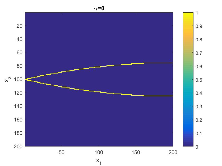
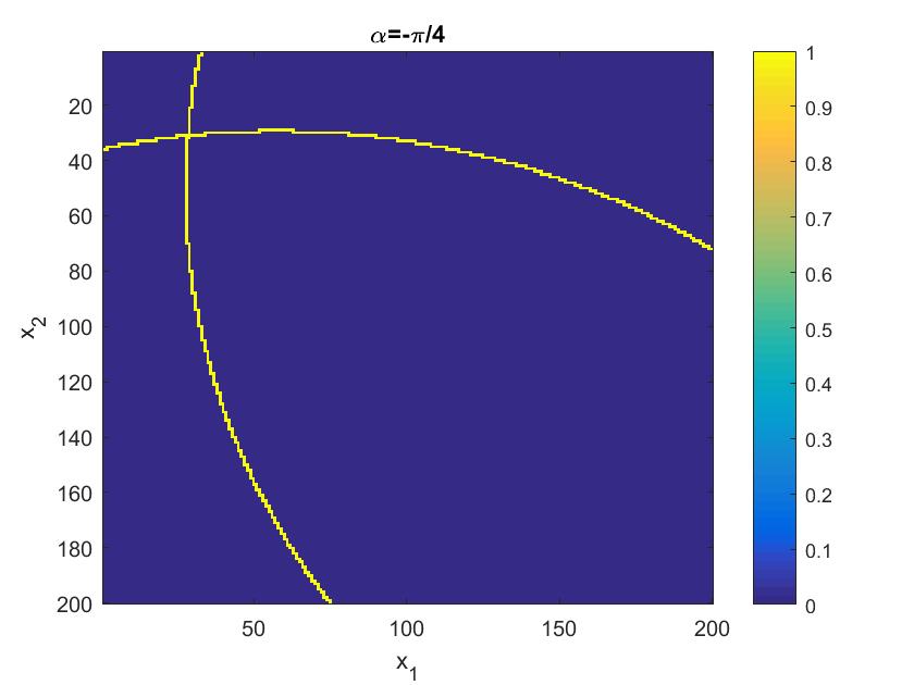
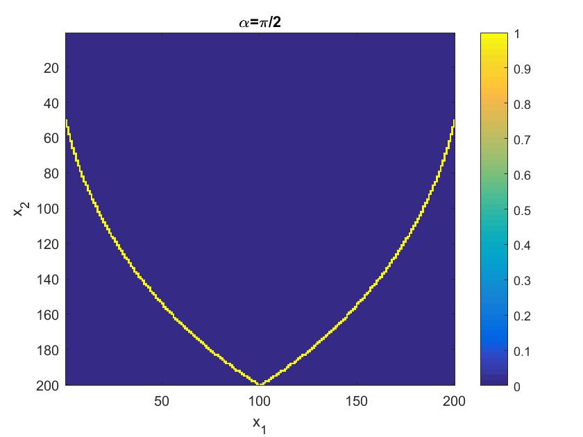
Figure 11: Discretized toric section integrals for varying rotation angles $\alpha$ and radii $r$ are presented as images. The images are binary (the pixel value is 1 if it intersected by a toric section and 0 otherwise).

We take a discrete (algebraic) approach to reconstruction. That is we discretize the operator $\mathcal{T}$ on a pixel grid (see figure 11) and find

(41) $$\operatorname*{arg\,min}_{\mathbf{v}}\|A\mathbf{v}-b\|^{2}_{2}+\lambda^{2}\mathcal{G}(\mathbf{v}),$$

where $A$ is the discrete form of $\mathcal{T}$ (each row of $A$ is the vectorized form of a binary image as shown in figure 11) and $\mathcal{G}(x)$ is a regularization penalty (e.g. $\mathcal{G}(\mathbf{v})=\|\mathbf{v}\|^{2}_{2}$ (Tikhonov) or $\mathcal{G}(\mathbf{v})=\sum_{i}|\mathbf{v}_{i}-\mathbf{v}_{i-1}|$ (TV)), with regularization parameter $\lambda$. Here $\mathbf{v}$ represents the vectorized form of the density image (which is to be reconstructed) and $b$ (our data) represents the Compton scattered intensity.

To simulate noisy data we take a vectorized density image $x$ (such as those presented in figure 6) we add a Gaussian random noise

(42) $$\mathbf{b}=A\mathbf{v}+\epsilon\times\frac{\mathbf{g}\|A\mathbf{v}\|_{2}}{\sqrt{n}},$$

where $\mathbf{g}$ is a pseudo-random vector of samples drawn from a standard normal distribution and $n$ is the number of entries in $\mathbf{b}$. Here $\epsilon$ denotes the noise level in the sense that

$$\frac{\|\mathbf{b}-A\mathbf{v}\|_{2}}{\|A\mathbf{v}\|_{2}}\approx\epsilon$$

for $n$ large enough. It is noted that simulating data as in (42) can often lead to optimistic results (due to the inverse crime). In appendix B we present additional reconstructions of a“multiple ring” phantom using analytically generated toric integral data, to avoid the inverse crime. The ring phantom $f$ is such that a closed form for $\mathcal{T}f$ is possible. For the more general phantoms considered later in this section, we have not found such a closed form. Hence in the main text, we choose to simulate the data as in (42). We shall see later (in figure 4) that the artefacts predicted by our microlocal theory are present using (42) for data simulation, so such a data generation is sufficient to verify our theoretical results.

Throughout the simulations presented here we simulate toric section integral data for rotation angles $\alpha\in\left\{\frac{j\pi}{180}:1\leq j\leq 360\right\}$ and for circle radii $r\in\left\{\frac{j^{2}+200^{2}}{2j}:1\leq j\leq 199\right\}$, where the pixel grid size is 200–200. So $n=360\times 199=71640$ and $A$ has $200^{2}$ columns.

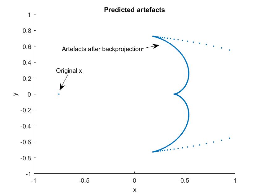
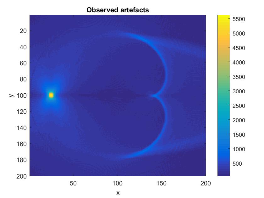
Figure 3: Predicted and observed artefacts from reconstructing a delta function far from the origin by backprojection.

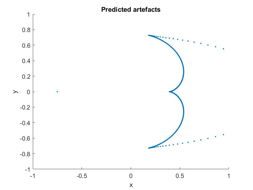
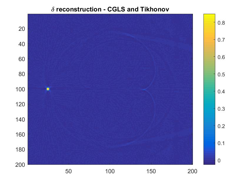
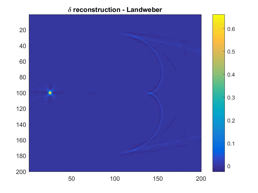
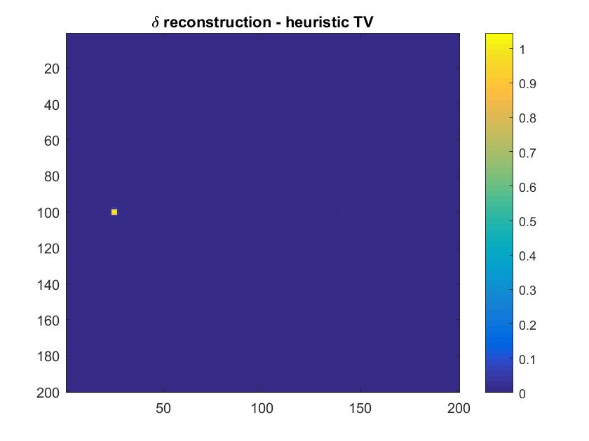
Figure 4: Reconstructions of a delta function with $5\%$ added noise. Top left – Predicted artefacts. Top right – CGLS and Tikhonov. Bottom left – Landweber. Bottom right – heuristic TV.

To simulate the artefacts implied by the theory presented in section 3.1, we consider the reconstruction of a delta function by (unfiltered) backprojection. That is by an application of the normal operator $\mathcal{T}^{*}\mathcal{T}\delta$, where $\delta$ has its support in the unit ball. To calculate the artefacts induced by $\Lambda_{1}=\widetilde{\mathcal{C}}_{1}^{t}\circ\mathcal{C}_{2}$ and $\Lambda_{2}=\widetilde{\mathcal{C}}_{2}^{t}\circ\mathcal{C}_{1}$ (as in Theorem 3.6) when $f=\delta$ (so here $f$ is non zero only at a single point and its wavefront set lies in all directions), let us consider a point $\mathbf{x}=|\mathbf{x}|(-1,0)$ on the $x$ axis. Then equation (30) becomes

(43) $$\mathbf{y}=\left(1+\frac{2}{s}\sin\alpha\cos\alpha,\frac{2}{s}\sin^{2}\alpha\right)^{T}$$

up to scaling. Similarly for $\mathbf{y}=|\mathbf{y}|(-1,0)$ equation (28) becomes

(44) $$\mathbf{x}=\left(1-\frac{2}{s}\sin\alpha\cos\alpha,-\frac{2}{s}\sin^{2}\alpha\right)^{T},$$

again up to scaling. Let us define $\psi_{1}:[0,\pi]\to\text{sg}(\mathbb{R}^{2})$ and $\psi_{2}:[-\pi,0]\to\text{sg}(\mathbb{R}^{2})$ as

(45) $$\psi_{1}(\alpha)=\left\{\nu\left(1-\frac{2}{s}\sin\alpha\cos\alpha,-\frac{2}{s}\sin^{2}\alpha\right):\nu\in\mathbb{R}\right\}\cap C_{1}\cap\left\{\mathbf{x}\cdot\theta_{\alpha}<0\right\}.$$

and

(46) $$\psi_{2}(\alpha)=\left\{\nu\left(1+\frac{2}{s}\sin\alpha\cos\alpha,\frac{2}{s}\sin^{2}\alpha\right):\nu\in\mathbb{R}\right\}\cap C_{2}\cap\left\{\mathbf{x}\cdot\theta_{\alpha}>0\right\}$$

where $\text{sg}(\mathbb{R}^{2})$ denotes the set of singleton subsets of $\mathbb{R}^{2}$. Also

(47) $$s=\left|\frac{3-|\mathbf{x}|^{2}+2(\mathbf{x}\cdot\theta)}{2(\mathbf{x}\cdot\theta_{\alpha})}\right|,$$

to get $s$ in terms of $\mathbf{x}$ and a rotation $\alpha$. Then $\psi_{1}([0,\pi])$ and $\psi_{2}([-\pi,0])$ are the set of artefacts in the plane associated to $\Lambda_{1}$ and $\Lambda_{2}$ respectively. Note that we need only consider the domain $[0,\pi]$ for $\psi_{1}$ as the circle $C_{1}$ does not intersect $\mathbf{x}=|\mathbf{x}|(-1,0)$ for any $\alpha\in(0,\pi)$, and conversely for $\psi_{2}$. It is clear that $\psi_{1}([0,\pi])=P\psi_{2}([-\pi,0])$, where $P$ denotes a reflection in the line $\{t\mathbf{x}:t\in\mathbb{R}\}$ (or the $x$ axis in this case). Hence the artefacts associated to $\Lambda_{1}$ are those associated to $\Lambda_{2}$ but reflected in the line $\{t\mathbf{x}:t\in\mathbb{R}\}$, for a given $\mathbf{x}\in\mathbb{R}^{2}$, when $f$ has singularities at $\mathbf{x}$ in all directions $\xi$. We can use equations (46) and (45) to draw curves in the plane where we expect there to be image artefacts. To simulate $\delta$ discretely we assign a value of 1 to nine neighbouring pixels in the unit cube (discretized as a 200–200 grid) and set all other pixel values to zero. Let our discrete delta function be denoted by $\mathbf{v}_{\delta}$. Then we approximate $\mathcal{T}^{*}\mathcal{T}\delta\approx A^{T}A\mathbf{v}_{\delta}$.

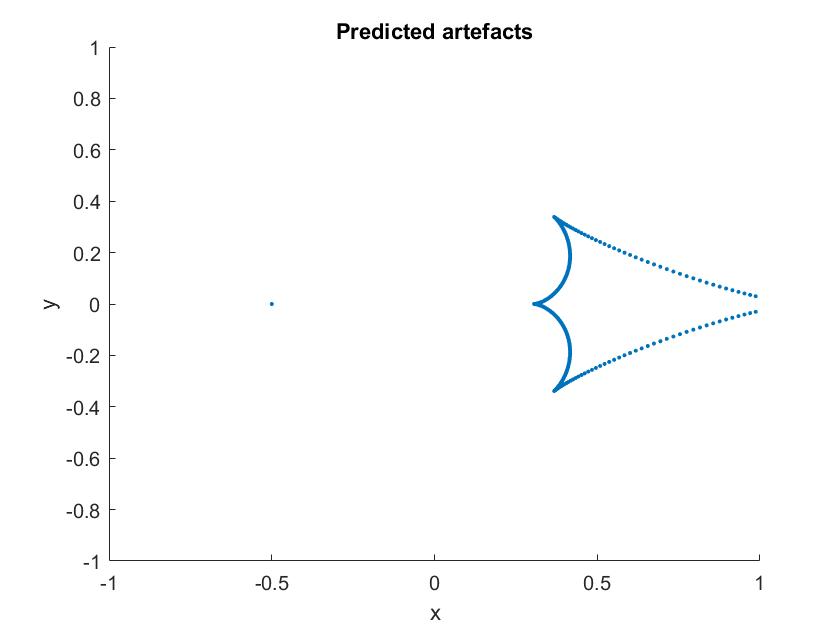
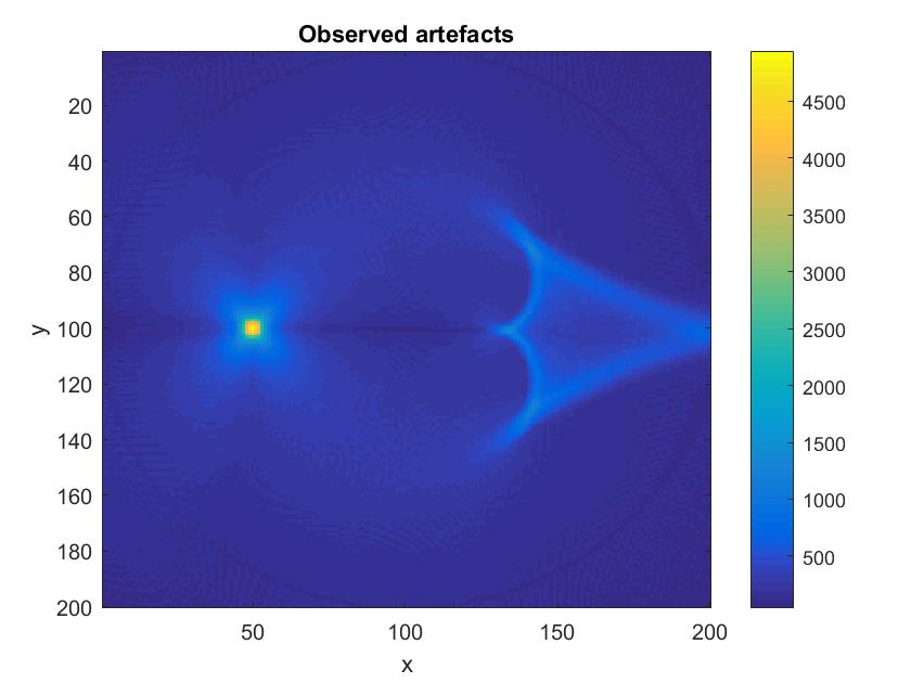
Figure 5: Predicted and observed artefacts from reconstructing a delta function closer to the origin by backprojection.

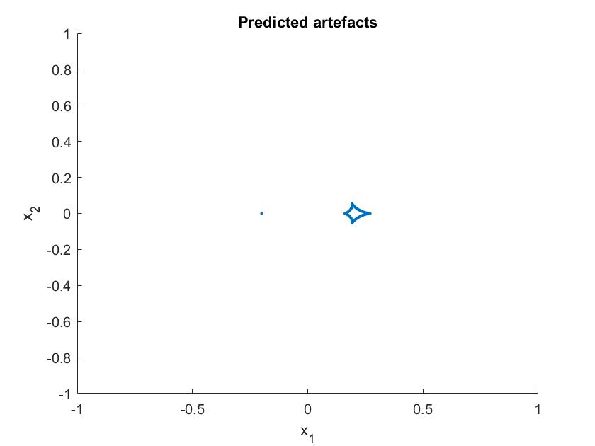
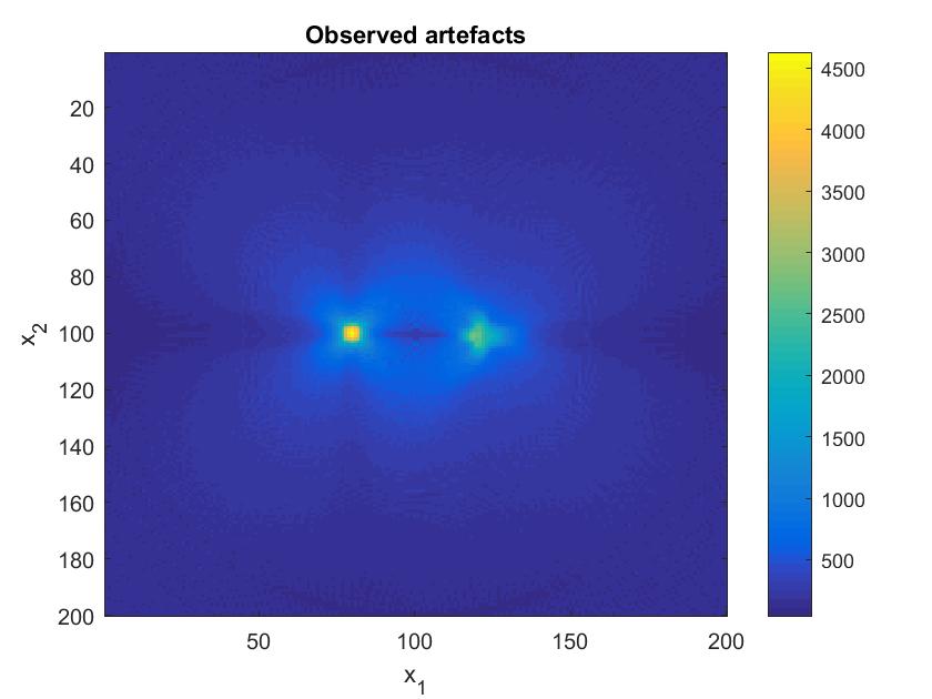
Figure 12: Predicted and observed artefacts from reconstructing a delta function close to the origin by backprojection.

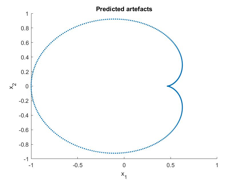
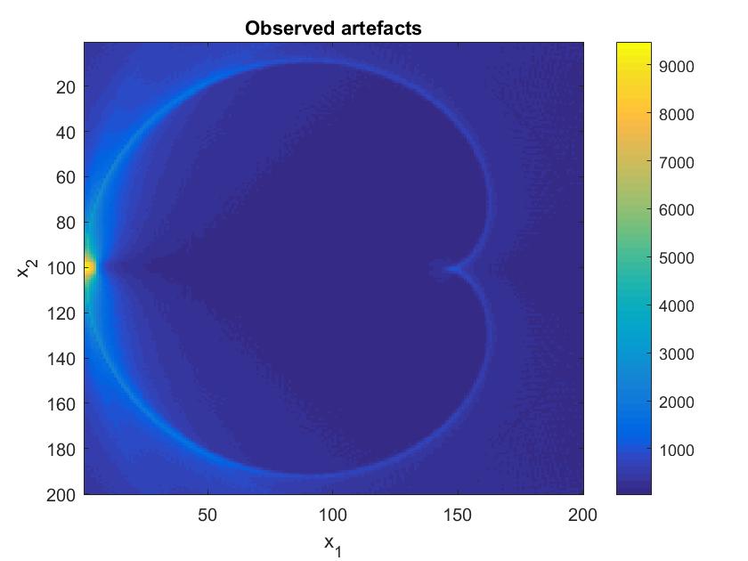
Figure 13: Predicted and observed artefacts from reconstructing a delta function on the boundary of the unit ball by backprojection. The artefacts are described by a cardioid.

See figures 3 and 5, where we have shown side by side comparisons of the artefacts predicted by equations (46) and (45) and the artefacts observed in a reconstruction by backprojection. See also figures 12 and 13 for more simulated artefact curves. Note that the blue dots in the left hand figures are the outputs of $\psi_{1}$ for $\alpha\in\left\{\frac{j\pi}{180}:1\leq j\leq 180\right\}$ and $\psi_{2}$ for $\alpha\in\left\{-\frac{j\pi}{180}:1\leq j\leq 180\right\}$. The observed artefacts are as predicted by the theory and the images in the left and right hand sides of each figure superimpose exactly. We notice a cardioid curve artefact in the reconstruction which becomes a full cardioid when the delta function lies approximately on the unit circle.

To test our reconstruction techniques, we consider the test phantoms displayed in figure 6, one simple and one complex.

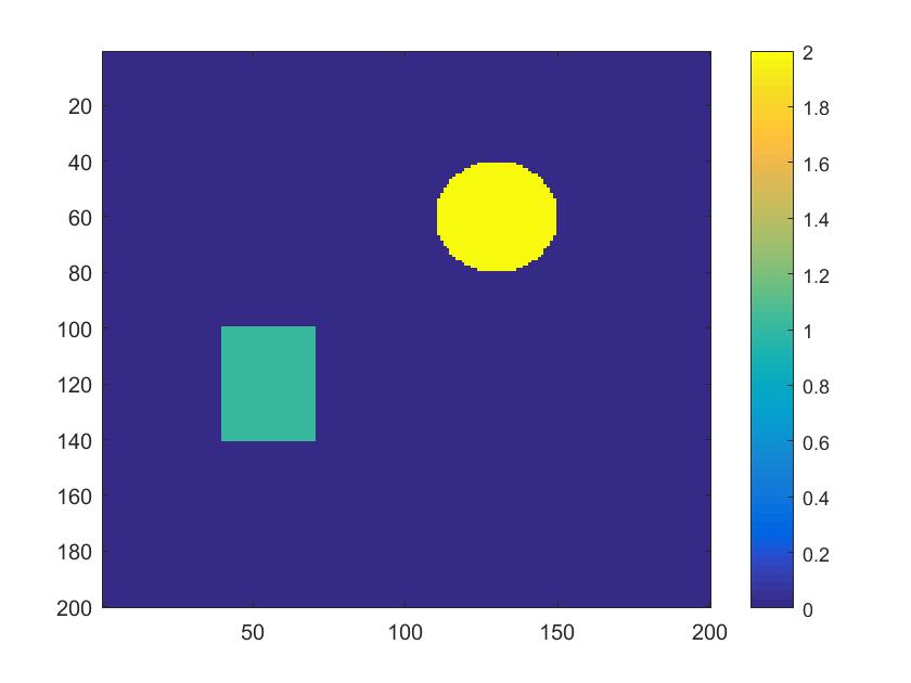
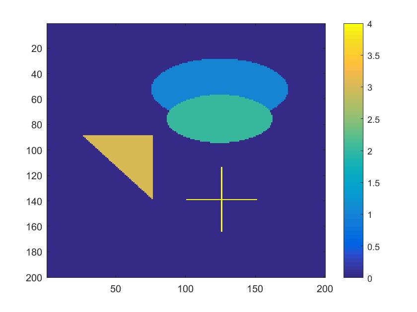
Figure 6: Simple (left) and complex (right) phantoms.

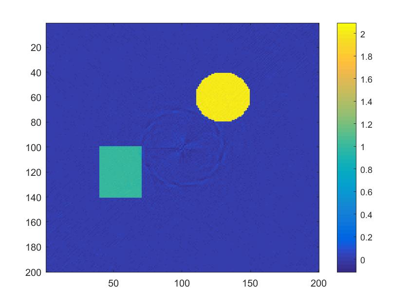
Figure 14: Reconstruction of simple phantom function using Landweber method and CGLS. No noise. Artefacts are present in Landweber iteration.

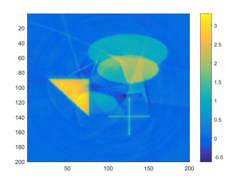
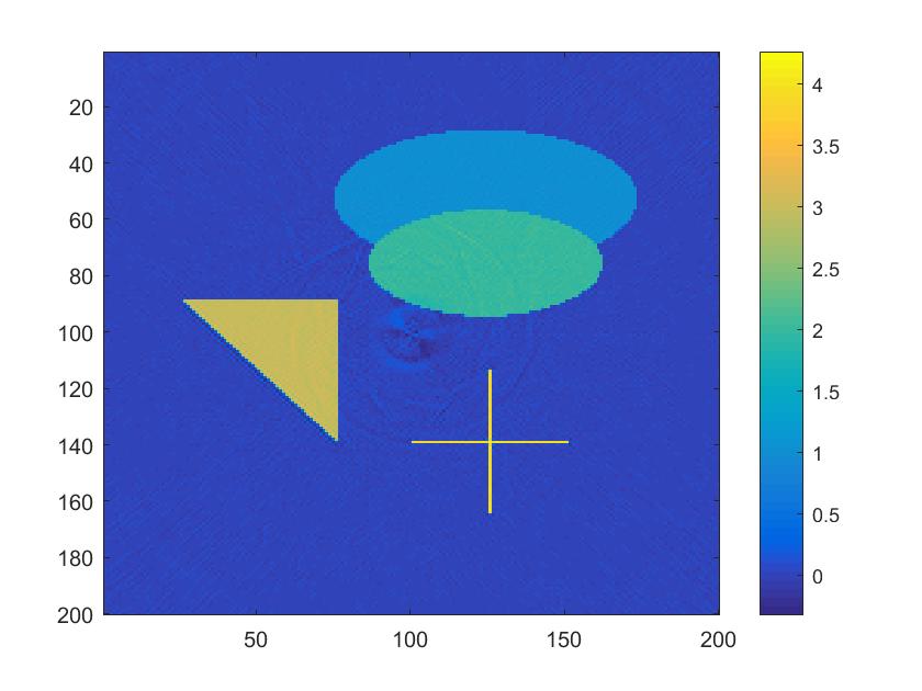
Figure 15: Reconstruction of complex phantom function using Landweber method and CGLS. No noise. Artefacts are present in Landweber iteration.

The simple phantom consists of a disc with value 2 and a square with value 1. The complex phantom consists of simulated objects of varying density, shape and size with overlapping ellipsoids, and is commonly used to test reconstruction techniques in tomography [8]. See figures 7, 8, 14, 15 for reconstructions of the two test phantoms using the Landweber method and a Conjugate Gradient Least Squares (CGLS) iterative solver [8] with Tikhonov regularization (varying the regularization parameter $\lambda$ manually). In the absence of noise ($\epsilon=0$) there are significant artefacts in the reconstruction using a Landweber approach. CGLS performs well however on both test phantoms. In the presence of added noise (we consider noise levels of $1\%$ ($\epsilon=0.01$) and $5\%$ ($\epsilon=0.05$)) there are severe artefacts in the reconstruction using a CGLS with Tikhonov approach (see figures 7 and 8), particularly with a higher noise level of $5\%$.

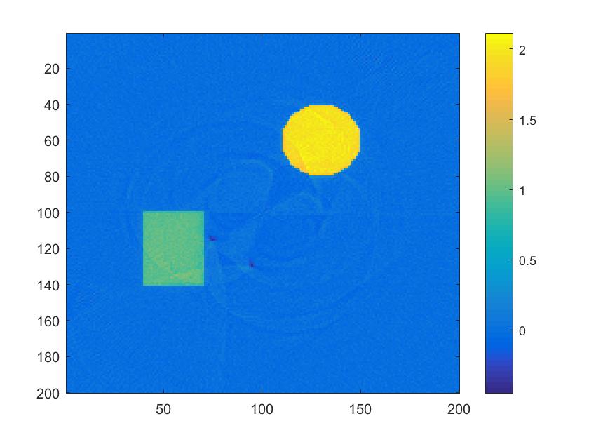
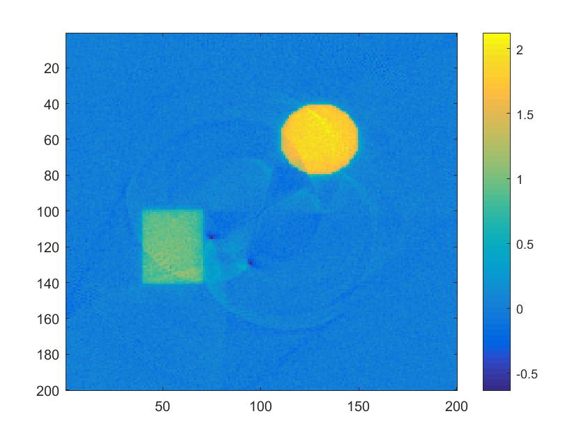
Figure 7: Simple phantom reconstruction using CGLS and Tikhonov as a regularizer, with noise levels of $1\%$ (left) and $5\%$ (right).

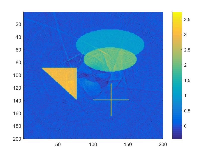
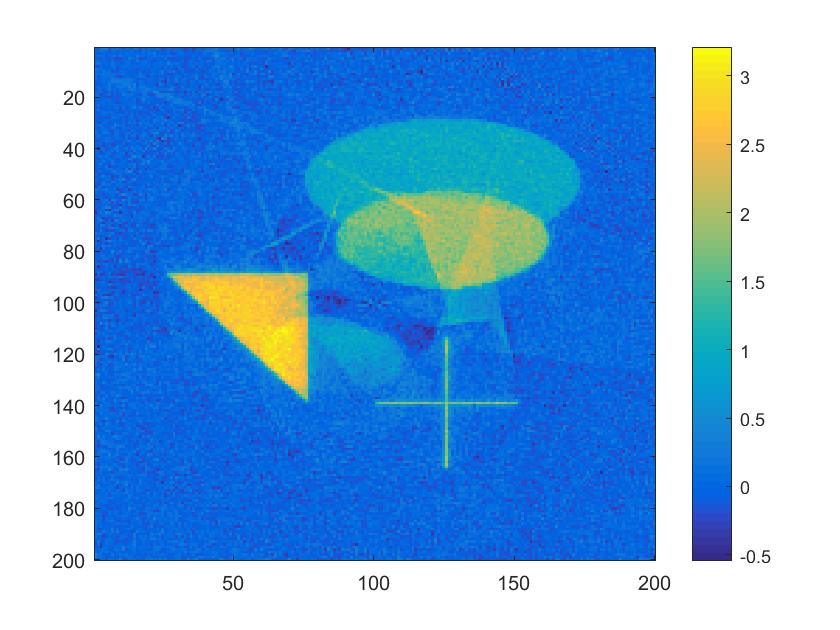
Figure 8: Complex phantom reconstruction using CGLS and Tikhonov as a regularizer, with noise levels of $1\%$ (left) and $5\%$ (right).

To combat the image artefacts we found that the use of an iterative approach with heuristic TV regularization (as described in [5]) was effective. Specifically we apply the method “IRhtv” of [5] with added non–negativity constraints to the optimizer (as we know a–priori that a density is non–negative), and choose the regularization parameter $\lambda$ manually. For more details on the IRhtv method see [6]. See figures 9 and 10.

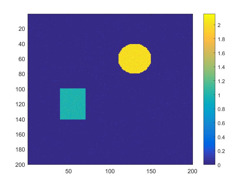
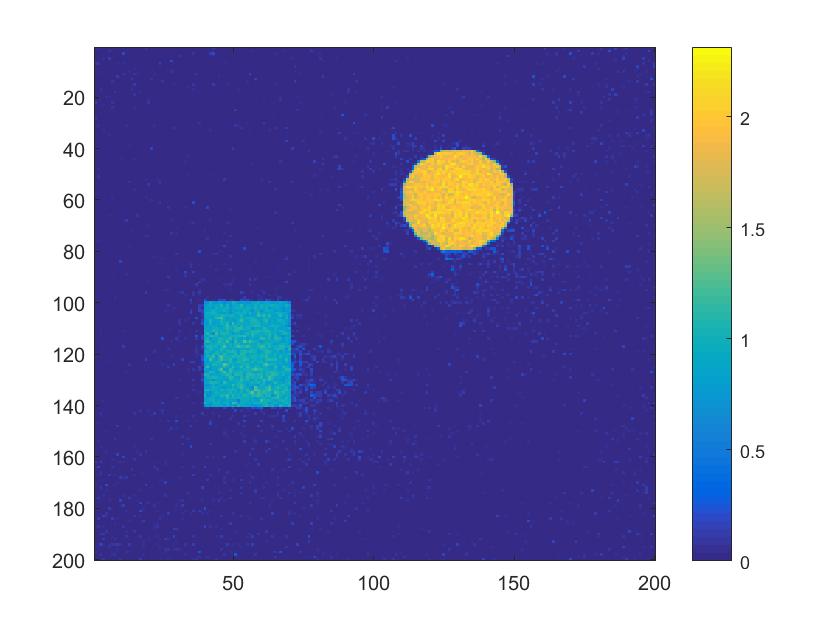
Figure 9: Simple phantom reconstruction using a heuristic TV regularizer, with noise levels of $1\%$ (left) and $5\%$ (right).

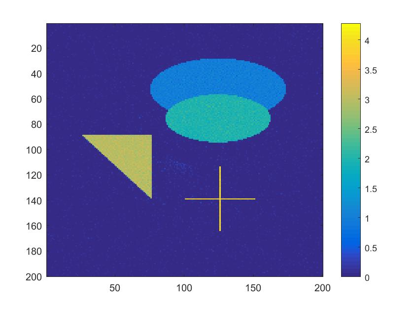
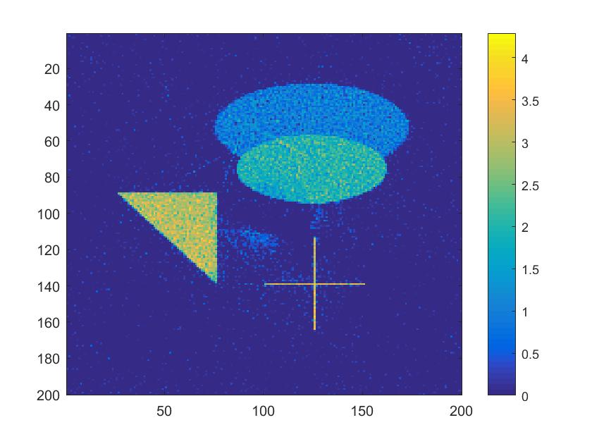
Figure 10: Complex phantom reconstruction using a heuristic TV regularizer, with noise levels of $1\%$ (left) and $5\%$ (right).

For a noise level of $1\%$ the artefacts are almost completely removed from the reconstructions (for both the simple and complex phantom) and the image quality is high overall. For a higher noise level of $5\%$ we see a significant reduction in the artefacts and the reconstruction is satisfactory in both cases with a low level of distortion in the image (although there is a higher distortion in the complex phantom reconstruction).

The predicted artefacts of figures 3 and 5 are also observed in a discrete reconstruction. See figure 4, where we have presented reconstructions of a delta function using the three iterative methods considered in this paper, namely CGLS with Tikhonov, a Landweber iteration and the solvers of [5] with heuristic TV. The artefacts of figure 3 can be observed faintly in the reconstruction using CGLS, and are most pronounced in the Landweber iteration. The heuristic TV approach gives the best performance (as before), although the reconstruction quality is more comparable among the three methods considered for a simple phantom such as a delta function.

For the application considered in this paper, namely threat detection in airport baggage screening, the removal of image artefacts and an accurate quantitative density estimation are crucial to maintain a satisfactory false positive rate. We will now further compare our results using CGLS with Tikhonov and the iterative solver of [5], in terms of the false positive rate we can expect using both methods. Looking at the reconstructions using both methods qualitatively. In figure 8 (using CGLS with Tikhonov), the image artefacts visually mask the four shapes which make up the original density. This may lead to threat materials or objects being misidentified (false negative errors). In addition, the artefacts introduce new “fake” densities (e.g. streaks in the top left of the image) to the original, which may be wrongly interpreted as a potential threat by security personnel (a false positive error). In figure 10 (using the iterative solver of [5]), with only a mild distortion in the image, we are less prone to such mistakes.

For a brief quantitative analysis, let the “cross” shaped object (with relative density 4) represent a detonator element and let the “triangular” density (with relative density 3) represent a small plastic explosive. Then the presence of artefacts can introduce large errors in the density estimation. For example, let us consider the left hand image in figure 8. if we take the average pixel value of the reconstructed explosive and detonator, then the relative errors are

(48) $$\text{errT}=100\times\frac{|\text{avgT}-3|}{3}=9.31\%,\ \ \ \ \text{errC}=100\times\frac{|\text{avgC}-4|}{4}=43.9\%,$$

where $\text{avgT}=2.72$ and $\text{avgC}=2.25$ are the average pixel values for the reconstructed plastic explosive and detonator element respectively. Let us say we were using a look up table approach to threat detection (which is a common approach). That is we look for densities (of a large enough size) in a pre–specified set of values and flag these as a potential threat. In threat detection, we cannot allow any false negatives, so if the above error rates were as expected the space of potential threats (the set of suspicious density values) would have to be increased (to allow for errors up to $44\%$) in order to compensate and identify the explosive, thus increasing the false positive rate.

If we now consider the same error rates for the left hand image in figure 10, then

(49) $$\text{errT}=100\times\frac{|\text{avgT}-3|}{3}=0.27\%,\ \ \ \ \text{errC}=100\times\frac{|\text{avgC}-4|}{4}=2.00\%,$$

where in this case $\text{avgT}=2.99$ and $\text{avgC}=3.92$. With such a reduction in the error rate, we can safely reduce the space of potential threats (now only allowing for errors less than $2\%$) in our look up table and hence reduce the expected false positive rate.

5 Conclusion

Here we have introduced a new toric section transform $\mathcal{T}$ which describes a two dimensional Compton tomography problem in airport baggage screening. A novel microlocal analysis of $\mathcal{T}$ was presented whereby the reconstruction artefacts were explained through an analysis of the canonical relation. This was carried out by an analysis of two circle transforms $\mathcal{T}_{1}$ and $\mathcal{T}_{2}$, whose canonical relations ($\mathcal{C}_{1}$ and $\mathcal{C}_{2}$) were shown to satisfy the Bolker Assumption when considered separately. When we considered their disjoint union ($\mathcal{C}=\mathcal{C}_{1}\cup\mathcal{C}_{2}$), which describes the canonical relation of $\mathcal{T}$, this was shown to be 2–1. We gave explicit expressions for the image artefacts implied by the 2–1 nature of $\mathcal{C}$ in section 3.1.

The injectivity of $\mathcal{T}$ was proven on the set of $L^{\infty}$ functions $f$ with compact support in $B$. Here we used the parameterization of circular arcs given by Nguyen and Truong in [18] to decompose $\mathcal{T}f$ in terms of orthogonal special functions (exploiting the rotational symmetry of $\mathcal{T}f$), and then applied similar ideas to those of Cormack [2] to prove injectivity.

In section 4 we presented a practical reconstruction algorithm for the reconstruction of densities from toric section integral data using an algebraic approach. We proposed to discretize the linear operator $\mathcal{T}$ on pixel grids (with the discrete form of $\mathcal{T}$ stored as a sparse matrix) and to solve the corresponding set of linear equations by minimizing the least squares error with regularization. To do this we applied the iterative techniques included in the package [5] and provided simulated reconstructions of two test phantoms (one simple and one complex) with varying levels of added pseudo-random noise. Here we demonstrated the artefacts explained by our microlocal analysis through a discrete application of the normal operator of $\mathcal{T}$ to a delta function, and showed (with a side by side comparison) that the artefacts in the reconstruction were exactly as predicted by our theory. We also showed that we could combat the artefacts in the reconstruction effectively using an iterative solver with a heuristic total variation penalty (using the code included in [5] for solving large scale image reconstruction problems), and explained how the improved artefact reduction implies a reduction in the false positive rate in the proposed application in airport baggage screening.

For further work we aim to consider more general acquisition geometries for the reconstruction of densities from toric section integral data in Compton scattering tomography. Here we have considered the particular three dimensional set of toric sections which describe the loci of scatterers for an idealised geometry for an airport baggage scanner. We wonder if the 2–1 nature of the canonical relation (or reflection artefacts) will be present for other toric section transforms and we aim to say something more concrete about this. For example, are reflection artefacts present or is the canonical relation 2–1 for any toric section transform?

Appendix A Potential application in airport baggage screening

Here we explain in more detail the proposed application in airport baggage screening, and how the theory and reconstruction methods presented in the main text relate to this field. In figure 16 we have displayed a machine configuration for RTT X-ray scanning in airport security screening (such a design is in use at airports today). The density $f$ is translated in the $x_{3}$ direction (out of the page) on a conveyor belt, and illuminated by a ring (the blue circle) of fixed-switched monochromatic (energy $E$) fan beam X-ray sources. The scattered intensity is then collected by a second ring (the green circle) of fixed energy-resolved detectors. The source and detector rings are coloured as in figures 1 and 2.

Figure 16: A security scanning machine configuration is displayed. The source-detector ring offset is small and is modelled as zero.

As is noted in the introduction (paragraph 3), the data are three dimensional. That is we can vary a source and detector position $(\mathbf{s},\mathbf{d})\in S^{1}\times S^{1}$ and the scattered energy $E^{\prime}$ (since the detectors are energy-resolved). We consider the two dimensional subset of this data, when $\mathbf{s}=-\mathbf{d}$. Varying the source position $\mathbf{s}$ (or $\mathbf{d}$) corresponds to varying $\theta$ as in section 3. The scattered energy $E^{\prime}$ determines $\cos\omega$ by equation (1) and in turn determines the torus radius

$$r=\frac{2}{\sqrt{1-\cos^{2}\omega}}.$$

The machine design of figure 16 has the ability to measure a combination of transmission (straight through photons) and scattered data. The photon counts measured when $E^{\prime}=E$ (unattenuated photons) correspond to line integrals over the attenuation coefficient $\mu_{E}$ (such as in standard transmission X-ray CT). The Compton scattered data (for $E^{\prime}<E$) determines the electron density $f=n_{e}$ (by the theory of section 3.2), and thus provides additional information regarding the physical properties of the scanned baggage. Hence we expect the use of the (extra) Compton data, in conjunction with the transmission data, to allow for a more accurate materials characterization (when compared to transmission or Compton tomography separately) and to ultimately lead to a more effective threat detection algorithm (e.g. reducing false positive rates in airport screening). Such ideas have already been put forward in [29], where a combination of $\mu_{E}$ and $n_{e}$ information is used to determine the effective atomic number of the material.

Appendix B Additional reconstructions with analytic data

Here we present additional reconstructions with analytically generated $\mathcal{T}f$ data, using the same reconstruction method as before, minimizing the functional (41). We consider the multiple ring phantom

(50) $$f(\mathbf{x})=\sum_{j=1}^{6}j\chi_{B_{10,15}}\left(\mathbf{x}-50\left(\cos\frac{j\pi}{3},\sin\frac{j\pi}{3}\right)\right)$$

as displayed in figure 17. Here $\chi_{S}$ denotes the characteristic function on $S$ and the reconstruction space is $[-100,100]^{2}$.

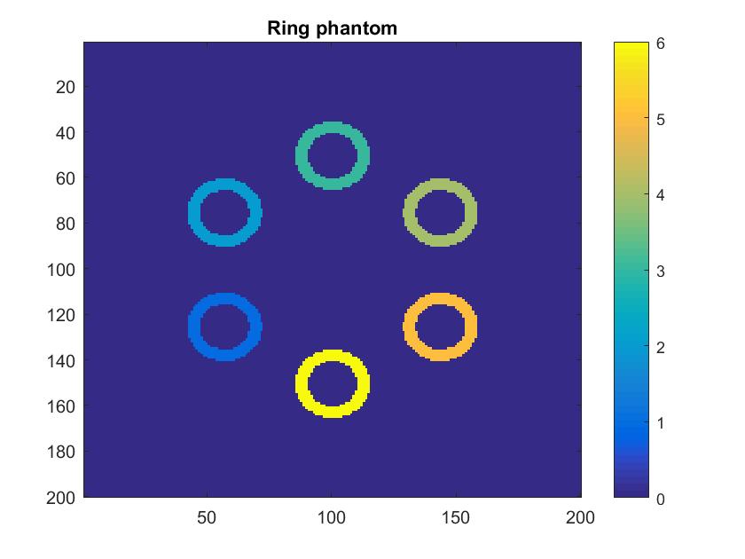
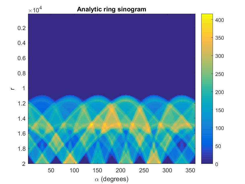
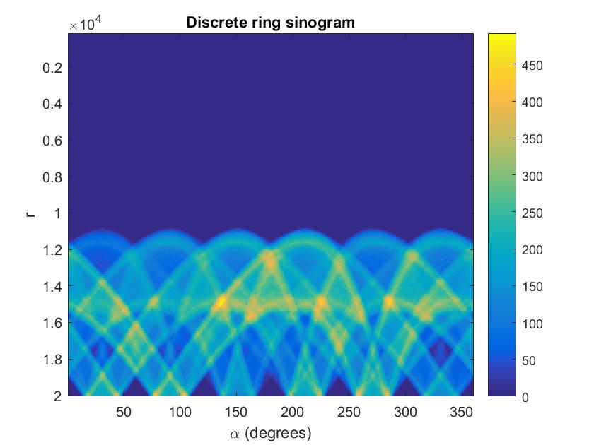
Figure 17: Ring phantom (left), analytic sinogram (middle) and discrete sinogram (right)

In this case the data are simulated as $\mathbf{b}=\mathcal{T}f(r,\alpha)$ for rotation angles $\alpha\in\left\{\frac{j\pi}{180}:1\leq j\leq 360\right\}$ and for circle radii $r\in\left\{\frac{j^{2}+200^{2}}{2j}:1\leq j\leq 199\right\}$ (as in section 4), and a Gaussian noise is added thereafter (as in equation (42)). See figure 17 for a comparison of the analytic and discrete sinogram data. The discrete sinograms were generated as before using $\mathbf{b}=A\mathbf{v}$ ($\mathbf{v}$ is the discrete form of $f$). The relative sinogram error is $\epsilon=\|\mathcal{T}f-A\mathbf{v}\|_{2}/\|\mathcal{T}f\|_{2}=0.11$, so in this case there is a significant (systematic) error due to discretization. See figure 18 for reconstructions of $f$ using the three methods considered in the main text, namely Conjugate Gradient Least Squares (CGLS) with Tikhonov, Landweber and heuristic Total Variation (TV). We present reconstructions using analytic data with added noise and discrete data with added noise for comparison. As in section 4 we see the best performance using heuristic TV. However there are additional artefacts in the analytic reconstructions due to discretization errors. Based on these experiments, it would be of benefit to construct the discrete form of $\mathcal{T}$ ($A$) from exact circle-pixel length intersections (as opposed to $A$ being a binary matrix). However we leave this for further work.

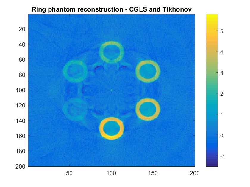
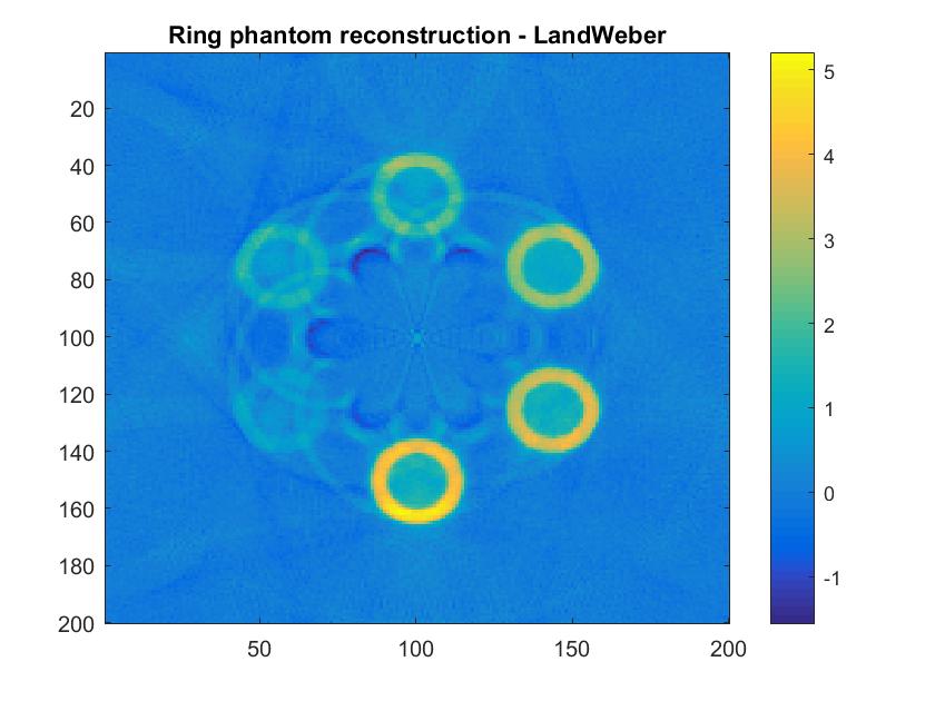
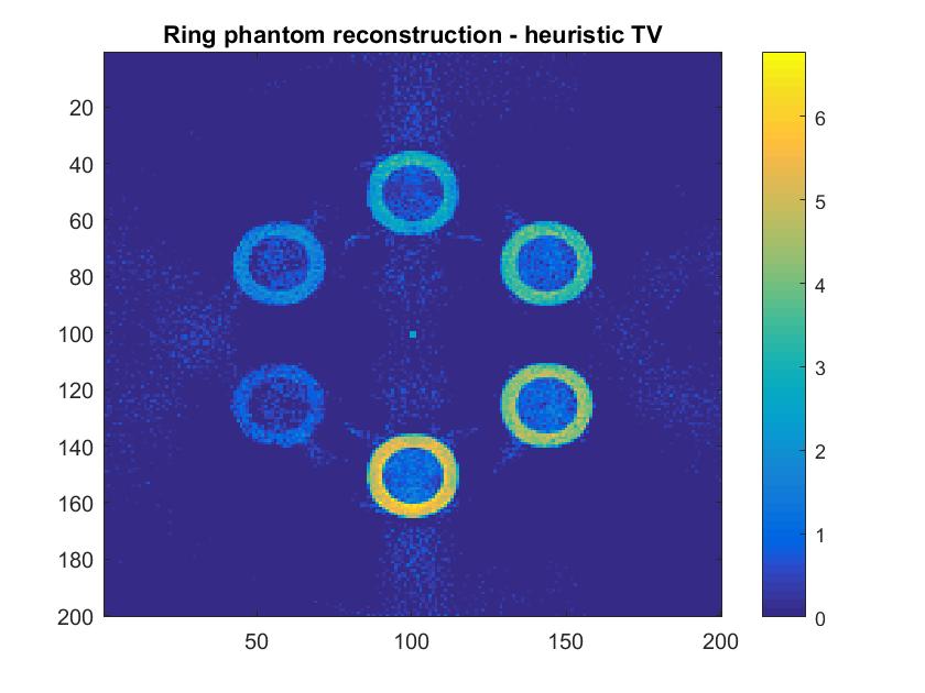
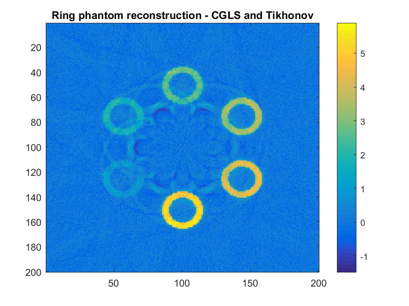
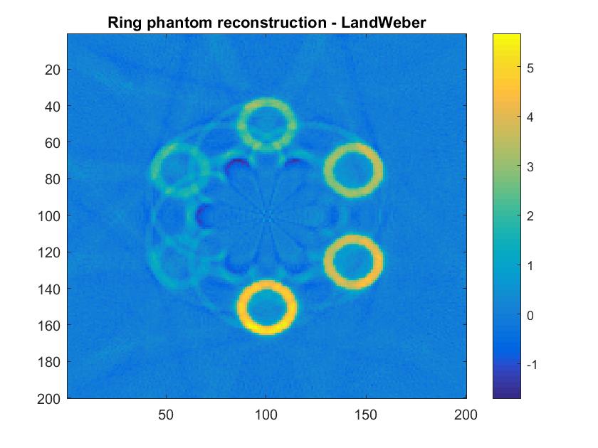
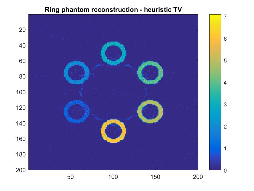
Figure 18: Top row – Reconstructions with analytic data plus $5\%$ noise. Bottom row – Reconstructions with discrete data plus $5\%$ noise (inverse crime).

References

- [1] L. Borg, J. Frikel, J. S. Jørgensen, and E. T. Quinto, Analyzing reconstruction artifacts from arbitrary incomplete X-ray CT data, SIAM J. Imaging Sci., 11 (2018), pp. 2786–2814, https://doi.org/10.1137/18M1166833.
- [2] A. M. Cormack, Representation of a function by its line integrals with some radiological applications, J. Appl. Physics, 34 (1963), pp. 2722–2727.
- [3] A. M. Cormack, Representation of a function by its line integrals with some radiological applications II, J. Appl. Physics, 35 (1964), pp. 2908–2913.
- [4] J. J. Duistermaat, Fourier integral operators, vol. 130 of Progress in Mathematics, Birkhäuser, Inc., Boston, MA, 1996.
- [5] S. Gazzola, P. C. Hansen, and J. G. Nagy, IR Tools: A MATLAB Package of Iterative Regularization Methods and Large-Scale Test Problems, 2017. arXiv preprint arXiv:1712.05602.
- [6] S. Gazzola and J. G. Nagy, Generalized Arnoldi–Tikhonov method for sparse reconstruction, SIAM Journal on Scientific Computing, 36 (2014), pp. B225–B247.
- [7] V. Guillemin and S. Sternberg, Geometric Asymptotics, American Mathematical Society, Providence, RI, 1977.
- [8] P. C. Hansen, Regularization Tools version 4.0 for Matlab 7.3, Numer. Algorithms, 46 (2007), pp. 189–194, https://doi.org/10.1007/s11075-007-9136-9.
- [9] P. C. Hansen and J. S. Jørgensen, AIR Tools II: algebraic iterative reconstruction methods, improved implementation, Numer. Algorithms, 79 (2018), pp. 107–137, https://doi.org/10.1007/s11075-017-0430-x, https://doi-org.ezproxy.library.tufts.edu/10.1007/s11075-017-0430-x.
- [10] M. Hoheisel, R. Bernhardt, R. Lawaczeck, and H. Pietsch, Comparison of polychromatic and monochromatic X-rays for imaging, Physics of Medical Imaging, 6142 (2006), p. 614209.
- [11] M. Hoheisel, R. Lawaczeck, H. Pietsch, and V. Arkadiev, Advantages of monochromatic x-rays for imaging, Physics of Medical Imaging, 5745 (2005), pp. 1087–1096.
- [12] A. J. Homan, Applications of microlocal analysis to some hyperbolic inverse problems, PhD thesis, Purdue University (United States), 2015. Open Access Dissertations. 473. https://docs.lib.purdue.edu/openaccessdissertations/473.
- [13] L. Hörmander, Fourier Integral Operators, I, Acta Mathematica, 127 (1971), pp. 79–183.
- [14] L. Hörmander, The analysis of linear partial differential operators. I, Classics in Mathematics, Springer-Verlag, Berlin, 2003. Distribution theory and Fourier analysis, Reprint of the second (1990) edition [Springer, Berlin].
- [15] L. Hörmander, The analysis of linear partial differential operators. III, Classics in Mathematics, Springer, Berlin, 2007, https://doi.org/10.1007/978-3-540-49938-1. Pseudo-differential operators, Reprint of the 1994 edition.
- [16] L. Hörmander, The analysis of linear partial differential operators. IV, Classics in Mathematics, Springer-Verlag, Berlin, 2009, https://doi.org/10.1007/978-3-642-00136-9. Fourier integral operators, Reprint of the 1994 edition.
- [17] F. Natterer, The mathematics of computerized tomography, Classics in Mathematics, Society for Industrial and Applied Mathematics (SIAM), New York, 2001.
- [18] M. Nguyen and T. T. Truong, Inversion of a new circular-arc Radon transform for Compton scattering tomography, Inverse Problems, 26 (2010), p. 065005.
- [19] C. J. Nolan and M. Cheney, Microlocal Analysis of Synthetic Aperture Radar Imaging, Journal of Fourier Analysis and Applications, 10 (2004), pp. 133–148.
- [20] S. J. Norton, Compton scattering tomography, Journal of applied physics, 76 (1994), pp. 2007–2015.
- [21] V. P. Palamodov, An analytic reconstruction for the Compton scattering tomography in a plane, Inverse Problems, 27 (2011), p. 125004.
- [22] E. T. Quinto, The dependence of the generalized Radon transform on defining measures, Trans. Amer. Math. Soc., 257 (1980), pp. 331–346.
- [23] E. T. Quinto, The invertibility of rotation invariant Radon transforms, J. Math. Anal. Appl., 94 (1983), pp. 602–603.
- [24] G. Rigaud, Compton scattering tomography: feature reconstruction and rotation-free modality, SIAM J. Imaging Sci., 10 (2017), pp. 2217–2249, https://doi.org/10.1137/17M1120105, https://doi.org/10.1137/17M1120105.
- [25] G. Rigaud and B. Hahn, 3D Compton scattering imaging and contour reconstruction for a class of Radon transforms, Inverse Problems, 34 (2018), pp. 075004, 22 pp.
- [26] P. Stefanov and G. Uhlmann, Is a curved flight path in SAR better than a straight one?, SIAM J. Appl. Math., 73 (2013), pp. 1596–1612, https://doi.org/10.1137/120882639.
- [27] W. M. Thompson, Source Firing Patterns and Reconstruction Algorithms for a Switched Source, Offset Detector CT Machine, PhD thesis, The University of Manchester (United Kingdom), 2011.
- [28] F. G. Tricomi, Integral Equations, Dover Books on Advanced Mathematics, Dover, New York, 1957.
- [29] J. Webber, X-ray Compton scattering tomography, Inverse problems in science and engineering, 24 (2016), pp. 1323–1346.
- [30] J. W. Webber and S. Holman, Microlocal analysis of a spindle transform, Inverse Problems & Imaging, 13 (2019), pp. 231–261, https://doi.org/10.3934/ipi.2019013, http://aimsciences.org//article/id/7ad5560c-e076-4384-9e9d-1dab4121da6d.
- [31] J. W. Webber and W. R. Lionheart, Three dimensional Compton scattering tomography, Inverse Problems, 34 (2018), p. 084001.
- [32] K. Yoshida, Lectures on Differential and Integral Equations, vol. 10 of Pure and Applied Mathematics, Interscience Publishers, New York, 1960.