The fine structure of Weber’s hydrogen atom –
Bohr-Sommerfeld approach

Abstract

In this paper we determine in second order in the fine structure constant the energy levels of Weber’s Hamiltonian admitting a quantized torus. Our formula coincides with the formula obtained by Wesley using the Schrödinger equation for Weber’s Hamiltonian.

1 Introduction

Although Weber’s electrodynamics was highly praised by Maxwell [Max73, p. XI], see also [KTA94, Preface], it was superseded by Maxwell’s theory and basically forgotten. Different from Maxwell’s theory, which is a field theory, Weber’s theory is a theory of action-at-a-distance, like Newton’s theory. Weber’s force law can be used to explain Ampère’s law and Faraday’s induction law; see [KTA94, Ch. 4 Ch. 5]. Different from the Maxwell-Lorentz theory Ampère’s original law also predicted transverse Ampère forces. Interesting experiments about the question of existence of transverse Ampère forces where carried out by Graneau and Graneau [GG96].

By quantizing the Coulomb potential Bohr and Sommerfeld, cf. [MR82, Ch. II], obtained for the hydrogen atom the following energy levels

$$-\frac{1}{2n^{2}},\quad n\in{\mathbb{N}},$$ (1.1)

in atomic units. Later Schrödinger interpreted these numbers as eigenvalues of his equation, cf.[MR87]. By taking account for velocity dependent mass, as suggested by Einstein’s theory of relativity, Sommerfeld obtained a more refined formula which also takes account of the angular momentum quantum number $\ell$. Sommerfeld’s formula [Som16, §2 Eq. (24)] is given in second order in the fine structure constant $\alpha$ by

$$-\frac{1}{2n^{2}}-\frac{\alpha^{2}}{2n^{3}\ell}+{\color[rgb]{0,0,0}\frac{3}{8}}\frac{\alpha^{2}}{n^{4}},\qquad n\in{\mathbb{N}},\quad\ell=1,\dots,n.$$ (1.2)

This formula, referred to as the fine structure of the hydrogen atom, coincides with the formula one derives in second order in $\alpha$ from Dirac’s equation as computed by Gordon [Gor28] and [Dar28]. We refer to Schweber [Sch94, §1.6] for the historical context of how Dirac discovered his equation.

The mathematical reason why the formula (1.1) of energy levels for the Coulomb potential of the Kepler problem is degenerate in the sense that it is independent of the angular momentum quantum number lies in the fact that the Coulomb problem is super-integrable. Namely, it is not just rotation invariant, but as well admits further integrals given by the Runge-Lenz vector. Dynamically this translates to the fact that for negative energy, except for collision orbits, all orbits are periodic. Indeed they are given by Kepler ellipses. While for velocity dependent mass rotation symmetry is preserved, the additional symmetry from the Runge Lenz vector is broken. Dynamically one sees that orbits are in general not any more periodic, but given by rosettes as illustrated by Figure 1. The situation for Weber’s Hamiltonian is quite analogous. In fact, Bush [Bus26] pointed out that the shapes of the orbits in both theories coincide. However, note even when the shapes of the orbits are the same this does not mean that their parametrization or their energy coincides.

In this paper we compute the energy levels of the Weber rosettes using Sommerfeld’s method.

Theorem A.

For Weber’s Hamiltonian the fine structure formula for the hydrogen atom in second order in the fine structure constant $\alpha$ becomes

$$-\frac{1}{2n^{2}}-\frac{\alpha^{2}}{2n^{3}\ell}+\frac{1}{2}\frac{\alpha^{2}}{n^{4}}.$$

Proof.

Equation (4.8). ∎

This formula coincides with the formula Wesley [Wes89, Eq. (100)] obtained using Schrödinger’s equation.
Note that the difference to Sommerfeld’s formula (1.2) involves $\alpha^{2}\approx 10^{-5}$ and only lies in the term just involving the main quantum number and not the angular one. Because this term is of much lower order than the Balmer term, i.e. the first term in (1.2), it seems difficult to actually measure the difference.

Outlook – Symplectic topology and non-local Floer homology

Weber’s Hamiltonian is related to delayed potentials as pointed out by Carl Neumann in 1868. We explain this relation in Appendix A. The question how to extend Floer theory to delayed potentials is a topic of active research, see [AFS18a, AFS18b, AFS18c]. In particular, for delayed potentials Floer’s equation is not local and therefore new analytic tools have to be developed inspired by the recent theory of polyfolds due to Hofer, Wysocki, and Zehnder [HWZ17]. While to our knowledge Weber’s Hamiltonian was so far unknown to the symplectic community, we hope to open up with this article a new branch of research in symplectic topology.

To our knowledge so far nobody incorporated the spin of the electron in Weber’s electrodynamics. In fact, it is even an amazing coincidence that Sommerfeld obtained the same formula for the fine structure of hydrogen as predicted by Dirac’s theory. It is explained by Keppeler [Kep03a, Kep03b] that using semiclassical techniques this can be explained, because the Maslov index and the influence of spin mutually cancelled out each other which both were not taken into account by Sommerfeld; neither in our paper. We expect that the proper incorporation of spin into Weber’s electrodynamics requires techniques from non-local Floer homology currently under development.

Lamb and Retherford [LR47] discovered 1947 that the spectrum of hydrogen shows an additional small shift not predicted by Dirac’s theory. This shift nowadays referred to as the Lamb shift was a major topic in the Shelter Island Conference and the driving force for the development of Quantum Field Theory and Renormalization Theory; see [Sch94, §4 §5]. An intuitive explanation of the Lamb shift is that vacuum fluctuations cause a small correction of the potential energy close to the nucleus and this small correction then leads to a shift in the spectrum of the hydrogen atom.

In Appendix A we explain following Neumann how a retarded Coulomb potential when Taylor approximated up to second order in the fine structure constant leads to Weber’s Hamiltonian. Higher order perturbations lead to perturbations of Weber’s Hamiltonian which are most strongly felt close to the nucleus. Whether there is a relation between these higher order perturbations and vacuum fluctuations is an important topic in the non-local Floer homology under development and its interaction with the semiclassical approach.

Acknowledgements. The authors would like to thank sincerely to André Koch Torres Assis for many useful conversations about Weber’s electrodynamics. The paper profited a lot from discussions with Peter Albers and Felix Schlenk about delay equations whom we would like to thank sincerely as well. This article was written during the stay of the first author at the Universidade Estadual de Campinas (UNICAMP) whom he would like to thank for hospitality. His visit was supported by UNICAMP and Fundação de Amparo à Pesquisa do Estado de São Paulo (FAPESP), processo $\mathrm{n}^{\rm o}$ 2017/19725-6.

2 Weber’s Hamiltonian

In this article we use atomic units to describe a model for the hydrogen atom. There are four atomic units which are unity: The electron mass $m_{e}=1$, the elementary charge $e=1$, the reduced Planck constant $\hbar=h/2\pi=1$, and the Coulomb force constant $k_{0}=1/(4\pi{\varepsilon}_{0})=1$. In particular, Coulomb’s Lagrangian and Hamiltonian for an electron ($-e=-1$) attracted by a proton are given by

$$L=\frac{1}{2}\mathopen{|}v\mathclose{|}^{2}+\frac{1}{\mathopen{|}q\mathclose{|}},\qquad H=\frac{1}{2}\mathopen{|}p\mathclose{|}^{2}-\frac{1}{\mathopen{|}q\mathclose{|}},$$

respectively. The speed of light is given in atomic units by $c=\frac{1}{\alpha}\approx 137$ where $\alpha$ is Sommerfeld’s fine structure constant. In his work Weber used a different constant, namely

$$c_{\rm W}=\sqrt{2}c.$$

In his famous experiment in 1856 he measured this constant together with Kohlrausch. This experiment was later crucial for Maxwell, because it indicated a strong relationship between electrodynamics and light [Web57].

The hydrogen atom consists of a (heavy) proton and a (light) electron. We just consider the planar case and suppose that the proton sits at the origin of ${\mathbb{R}}^{2}$. Polar coordinates $(r,\phi)\in{\mathbb{R}}^{2}_{\times}:={\mathbb{R}}^{2}\setminus\{0\}$ provide the coordinates $(r,\phi,v_{r},v_{\phi})\in T{\mathbb{R}}^{2}_{\times}$ and $(r,\phi,p_{r},p_{\phi})\in T^{*}{\mathbb{R}}^{2}_{\times}$. Consider the Lagrangian function

$$L_{\rm W}(r,\phi,v_{r},v_{\phi})=\underbrace{\frac{1}{2}(v_{r}^{2}+r^{2}v_{\phi}^{2})}_{=:T_{\rm flat}}+\underbrace{\frac{1}{r}\bigg{(}1+\frac{v_{r}^{2}}{2c^{2}}\bigg{)}}_{=:-S}$$ (2.3)

Here $T_{\rm flat}$ is just the kinetic energy in polar coordinates, while $S$ is referred in [KTA94] as the ’Lagrangian energy’. Note that $L_{\rm W}$ differs from the Coulomb Lagrangian $L$ by the additional term $v_{r}^{2}/2c^{2}r$. This Lagrangian was introduced by Carl Neumann [Neu68a] in 1868. We refer to $S$ as Neumann’s potential function. Its Euler Lagrange equation are precisely the equations studied by Wilhelm Weber [Web46] twenty years earlier in 1846. In Appendix A we explain how Neumann’s potential function can be obtained as Taylor approximation of a retarded functional.

Observe that the $S$ term in $L_{\rm W}$ depends on the velocity. Historically this led to a lot of confusion and so Helmholtz [Hel47] and Maxwell [Max55] doubted for a long time that Weber’s force law complies with conservation of energy; cf. [KTA94, §3.6]. In [TLKT67, §384/385] Weber’s theory was even classified under the theories “pernicious rather than useful.”
Although in 1871 Weber explained in detail that his force law satisfies the principle of preservation of energy, his article [Web71] was not mentioned in the translation [TLKT71] of Thompson and Tait’s book by Helmholtz and Wertheim which infuriated Zöllner [Zöl72, Vorrede] “Ich wage es zuversichtlich zu behaupten, dass in der ganzen deutschen Literatur nicht ein einziges Lehrbuch anzutreffen sein wird, welches wie jener berüchtigte §385 des Werkes von Thomson und Tait auf dem engen Raume von nur dreissig Zeilen eine solche Fülle von absolutem Nonsens enthält.” In the new edition of Thompson and Tait [TLKT79] the infamous $\S 385$ has disappeared.

A symplectic way to see that the disputed preservation of energy holds for Weber’s force law is to rearrange in (2.3) the brackets to obtain

$$L_{\rm W}(r,\phi,v_{r},v_{\phi}) = \frac{1}{2}\bigg{(}1+\frac{1}{c^{2}r}\bigg{)}v_{r}^{2}+\frac{1}{2}r^{2}v_{\phi}^{2}+\frac{1}{r}$$

$$= \frac{1}{2}\left(g_{rr}\,v_{r}^{2}+g_{\phi\phi}\,v_{\phi}^{2}\right)+\frac{1}{r}$$

$$= T-V.$$

The first term in the sum can be interpreted as kinetic energy with respect to a non-flat Riemannian metric $g$ on ${\mathbb{R}}^{2}_{\times}$, while the second term is minus the (velocity independent) Coulomb potential. In Appendix B we explain how in the case of two protons the metric becomes singular at Weber’s critical radius $\rho$. Outside this critical radius the metric is Riemannian, while inside it is Minkowski.

Legendre transformation ${\mathcal{L}}:T{\mathbb{R}}^{2}_{\times}\to T^{*}{\mathbb{R}}^{2}_{\times}$ of the mechanical Lagrangian $L=T-V$ yields the mechanical Hamiltonian

$$H_{\rm W}(r,\phi,p_{r},p_{\phi}) = T^{*}+V$$

$$= \frac{1}{2}\left(\frac{1}{g_{rr}}\,p_{r}^{2}+\frac{1}{g_{\phi\phi}}\,p_{\phi}^{2}\right)-\frac{1}{r}$$

$$= \frac{1}{2}\left(\frac{c^{2}r}{c^{2}r+1}\,p_{r}^{2}+\frac{1}{r^{2}}\,p_{\phi}^{2}\right)-\frac{1}{r}.$$

But this is an autonomous Hamiltonian and any such is preserved along its flow; see e.g. [MS17, p. 99]. This explains preservation of energy.

With the help of the fine structure constant $\alpha=\frac{1}{c}$ the Hamiltonian reads

$$H_{\rm W}(r,{\color[rgb]{.75,.5,.25}\phi},p_{r},p_{\phi})=\frac{1}{2}\frac{r}{r+\alpha^{2}}\,p_{r}^{2}+\frac{1}{2r^{2}}\,p_{\phi}^{2}-\frac{1}{r}.$$ (2.4)

We refer to $H_{\rm W}$ as Weber’s Hamiltonian.

3 Quantized tori

Weber’s Hamiltonian is completely integrable in the planar case under consideration. Indeed it is rotational invariant and therefore angular momentum commutes with $H_{\rm W}$.

On closed symplectic manifolds the Arnol^′d-Liouville theorem, see e.g. [HZ11, App. A.2], tells us how the manifold gets foliated by invariant tori. Even below the escape threshold, i.e. for negative energy, in the case at hand the tori might have some holes, because of collisions.
For the Kepler Hamiltonian collisions can be regularized. There exist different regularizations in the literature. For example, Moser showed in [Mos70] that for negative energies $E<0$ the Kepler flow after regularization can be identified with the geodesic flow on a $2$-dimensional sphere. For zero energy $E=0$ Kepler flow after regularization becomes identified with geodesic flow on the euclidean plane, for positive energy $E>0$ with the geodesic flow on hyperbolic space, as shown by Belbruno [Bel77] and Osipov [Osi77]; see also Milnor [Mil83]. Historically even older is the regularization by Goursat [Gou89] which was rediscovered independently by Levi-Civita [LC20] and is nowadays referred to as Levi-Civita regularization. Different from Moser, the Levi-Civita regularization is $2:1$ and transforms the Kepler flow for negative energy $E<0$ to the flow of two uncoupled harmonic oscillators.

To our knowledge so far nobody studied regularization for the Weber Hamiltonian and this would be an interesting project. Nevertheless, one can easily see how the invariant tori look like. Indeed for negative energy usual orbits, apart from circle orbits and collisions, are given by rosettes; see Figure 1.

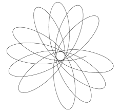
Figure 1: A rosette ($r=1+\kappa\cos\gamma\phi$, eccentricity $0<\kappa<1$)

Different from the Kepler problem where these orbits are given by Kepler ellipses, the rosettes don’t need to be closed and they show a perihel shift; see references in [WKTAW18, p. 56 footnote 37]. In the case at hand, where the central body is interpreted as a proton, let us replace the expression ’perihel shift’ by periproton shift. If the periproton shift is a rational multiple of $2\pi$, then the rosette finally closes and we obtain a periodic orbit. Hence by rotation invariance of $H_{\rm W}$ we obtain a circle family of periodic orbits by rotating our closed rosette. But a circle times a circle is a 2-dimensional torus. In this case the flow on the invariant torus is rational.

If the periproton shift is irrational, the rosette is not closed and we obtain the invariant torus by looking at the closure of the rosette. In this case the flow on the invariant torus is irrational.

A conceptual explanation what Bohr-Sommerfeld quantization of a completely integrable system is was given by Einstein [Ein17] in 1917; see also [Gut90, §14.1]. The invariant tori are Lagrangian. Hence if we consider the restriction of the Liouville 1-form to the torus $T$ it is closed and therefore it defines a class $[\lambda_{\rm can}]\in{\rm H}^{1}(T;{\mathbb{R}})$ in the first cohomology of the torus. If this class is integer-valued, then we call the torus a quantized torus. For some unknown reason the electron just likes to stay on quantized tori. Emission occurs if the electron jumps from one quantized torus to another one. In this case the frequency we observe is given by $\frac{1}{2\pi}$ times the energy difference of the two energy levels where the quantized tori lie.

Therefore to understand the spectrum of the electron we have to figure out which energy level contain a quantized torus. How to do this in practice is the content of Sommerfeld’s book [Som16].

In the next section we explain how one apply Sommerfeld’s calculations to the Weber Hamiltonian.

4 Bohr-Sommerfeld quantization

We quantize the Hamiltonian according to the rules of Bohr and Sommerfeld. Note that $H_{\rm W}$ does not depend on ${\color[rgb]{.75,.5,.25}\phi}$, so $p_{\phi}$ is a preserved quantity that corresponds to angular momentum. According to Bohr [Boh13] angular momentum has to be quantized: The angular momentum quantum number is

$$\frac{1}{2\pi}\int_{0}^{2\pi}p_{\phi}\,d\phi=p_{\phi}=:\ell\in{\mathbb{N}}.$$ (4.5)

Here the first identity holds by preservation of angular momentum. Later Sommerfeld referred to $\ell$ as the azimuthal quantum number which in his notation was called $n$. Originally Bohr just considered circular orbits and therefore the azimutal quantum number was enough. In contrast, Sommerfeld [Som16] allowed as well more general orbits and imposed a quantization condition on $p_{r}$ as well, namely

$$\frac{1}{2\pi}\int p_{r}\,dr=:n_{r}\in{\mathbb{N}}_{0}.$$

This integral has to be interpreted as follows. Note that because of rotational invariance (independence of $\phi$) of the Weber Hamiltonian $H_{\rm W}$, orbits in the configuration space are given by rosettes, i.e. the $r$ variable is periodic in time, oscillating between the periproton $r_{\rm min}$ and the apoproton $r_{\rm max}$ (closest/farthest point from proton). Therefore

$$\int p_{r}\,dr=2\int_{r_{\rm min}}^{r_{\rm max}}p_{r}\,dr.$$

How to interpret and calculate $\int_{r_{\rm min}}^{r_{\rm max}}p_{r}\,dr$ is illustrated by [Som21, p. 478 Fig. 101]. Using (2.4) and (4.5) we compute for $p_{r}$ the formula

$$p_{r} = \sqrt{2\bigg{(}1+\frac{\alpha^{2}}{r}\bigg{)}\bigg{(}H_{\rm W}+\frac{1}{r}-\frac{\ell^{2}}{2r^{2}}\bigg{)}}$$

$$= \sqrt{2H_{\rm W}+\frac{2+2\alpha^{2}H_{\rm W}}{r}-\frac{\ell^{2}-2\alpha^{2}}{r^{2}}-\frac{\ell^{2}\alpha^{2}}{r^{3}}}.$$

We abbreviate

$$A=2H_{\rm W},\quad B=1+\alpha^{2}H_{\rm W},\quad C=-\ell^{2}+2\alpha^{2}<0,\quad D_{1}=-\ell^{2}\alpha^{2}$$ (4.6)

so that $p_{r}$ becomes

$$p_{r}=\sqrt{A+\frac{2B}{r}+\frac{C}{r^{2}}+\frac{D_{1}}{r^{3}}}.$$

As calculated by Sommerfeld [Som21, p.480 (16)] the integral $n_{r}$ is given by

$$n_{r}=-i\left(\sqrt{C}-\frac{B}{\sqrt{A}}-\frac{BD_{1}}{2C\sqrt{C}}\right)$$

where as explained in [Som21, p.479] the square root of $C$ has to be taken negative imaginary, whereas the one of A positive. Plugging in (4.6) we obtain

$$n_{r} = -i\bigg{(}-i\sqrt{\ell^{2}-2\alpha^{2}}-\frac{1+\alpha^{2}H_{\rm W}}{\sqrt{2H_{\rm W}}}+\frac{(1+\alpha^{2}H_{\rm W})\ell^{2}\alpha^{2}}{2i(\ell^{2}-2\alpha^{2})^{3/2}}\bigg{)}$$

$$= -\sqrt{\ell^{2}-2\alpha^{2}}+i\frac{1+\alpha^{2}H_{\rm W}}{\sqrt{2H_{\rm W}}}-\frac{(1+\alpha^{2}H_{\rm W})\ell^{2}\alpha^{2}}{2(\ell^{2}-2\alpha^{2})^{3/2}}.$$

Taking the two imaginary terms to the left hand side shows that

$$n_{r}+\sqrt{\ell^{2}-2\alpha^{2}}+\frac{(1+\alpha^{2}H_{\rm W})\ell^{2}\alpha^{2}}{2(\ell^{2}-2\alpha^{2})^{3/2}}=i\frac{1+\alpha^{2}H_{\rm W}}{\sqrt{2H_{\rm W}}}.$$

By Taylor expansion of the left hand side in $(\alpha^{2})$ up to first order we get

$$\begin{split}n_{r}+\sqrt{\ell^{2}-2\alpha^{2}}+\frac{(1+\alpha^{2}H_{\rm W})\ell^{2}\alpha^{2}}{2(\ell^{2}-2\alpha^{2})^{3/2}}&\approx n_{r}+\ell-\frac{\alpha^{2}}{\ell}+\frac{\ell^{2}\alpha^{2}}{2\ell^{3}}\\ &=(n_{r}+\ell)-\frac{\alpha^{2}}{2\ell}.\end{split}$$ (4.7)

Plugging this formula into the previous formula and taking squares we obtain to first order in $(\alpha^{2})$ the approximation

$$(n_{r}+\ell)^{2}-\frac{\alpha^{2}(\ell+n_{r})}{\ell}\approx-\frac{1+2\alpha^{2}H_{\rm W}}{2H_{\rm W}}=-\frac{1}{2H_{\rm W}}-\alpha^{2}.$$

Rearranging we get

$$\frac{-1}{2H_{\rm W}}\approx(n_{r}+\ell)^{2}-\frac{\alpha^{2}n_{r}}{\ell}$$

and therefore, expanding again up to first order in $(\alpha^{2})$, we obtain

$$H_{\rm W} \approx -\frac{1}{2\big{(}(n_{r}+\ell)^{2}-\frac{\alpha^{2}n_{r}}{\ell}\big{)}}\approx-\frac{1}{2(n_{r}+\ell)^{2}}-\frac{\alpha^{2}n_{r}}{2(n_{r}+\ell)^{4}\ell}.$$

By introducing the main quantum number

$$n:=n_{r}+\ell\in{\mathbb{N}}$$

the previous formula becomes

$$H_{\rm W}\approx-\frac{1}{2n^{2}}-\frac{\alpha^{2}}{2n^{3}\ell}+\frac{\alpha^{2}}{2n^{4}}.$$ (4.8)

The corresponding formula for Sommerfeld’s relativistic Hamiltonian is

$$H_{\rm S}\approx-\frac{1}{2n^{2}}-\frac{\alpha^{2}}{2n^{3}\ell}+\frac{3\alpha^{2}}{8n^{4}}.$$

Appendix A Weber’s Lagrangian and delayed potentials

In several works Neumann treated the connection between Weber’s dynamics and delayed potentials, see [Neu68a, Neu68b] and [Neu96, Ch. 8]. Neumann explained how Weber’s potential function is related to Hamilton’s principle which in [Neu68b] he called “norma suprema et sacrosancta, nullis exceptionibus obvia”.

Strictly speaking, a delay potential only makes sense for loops and not for chords. Hence we abbreviate by $\mathcal{L}=C^{\infty}\big{(}S^{1},\mathbb{R}^{2}_{\times}\big{)}$ the free loop space on the punctured plane ${\mathbb{R}}^{2}_{\times}:=\mathbb{R}^{2}\setminus\{0\}$. For a potential $V\in C^{\infty}\big{(}\mathbb{R}^{2}_{\times},\mathbb{R}\big{)}$ and a constant $c_{\rm W}>0$ we define three functions

$${\mathcal{S}}_{\mathrm{kin}},{\mathcal{S}}_{\mathrm{pot}},{\mathcal{S}}\colon\mathcal{L}\to\mathbb{R}$$

by ${\mathcal{S}}={\mathcal{S}}_{\mathrm{kin}}-{\mathcal{S}}_{\mathrm{pot}}$ and by

$${\mathcal{S}}_{\mathrm{kin}}(q):=\frac{1}{2}\int_{0}^{1}|q^{\prime}(t)|^{2}dt,\qquad{\mathcal{S}}_{\mathrm{pot}}(q):=\int_{0}^{1}V\Big{(}q\Big{(}t-\tfrac{|q(t)|}{c_{\rm W}}\Big{)}\Big{)}dt.$$

Physically this means that the potential energy is evaluated at a retarded time. Namely, the position of the proton at the origin has to be transmitted to the electron at speed $c_{\rm W}$. It is a strange fact that to obtain Weber’s force this transmission velocity is given by the Weber constant $c_{\rm W}$ which, as measured by Weber and Kohlrausch [Web57], equals $\sqrt{2}c$ where $c$ is the speed of light.

We assume that $V$ only depends on the radial coordinate $V(q)=V(|q|)=V(r)$. Setting $r(t):=\mathopen{|}q(t)\mathclose{|}$ the functional ${\mathcal{S}}_{\mathrm{pot}}$ becomes a function of $r=r(t)$, still denoted by

$${\mathcal{S}}_{\mathrm{pot}}(r)=\int_{0}^{1}V\Big{(}r\Big{(}t-\tfrac{r(t)}{c_{\rm W}}\Big{)}\Big{)}dt.$$

We further abbreviate

$$a=\frac{1}{c_{\rm W}}=\frac{\alpha}{\sqrt{2}},\qquad c_{\rm W}=\sqrt{2}c,$$

where $\alpha$ is the fine structure constant.

Setting $V_{r}(a,t):=V\big{(}r\big{(}t-ar(t)\big{)}\big{)}$ we obtain for the partial derivatives in $a$ the formulas

$$\frac{\partial}{\partial a}V_{r}(a,t)=-V^{\prime}\big{(}r\big{(}t-ar(t)\big{)}\big{)}r^{\prime}\big{(}t-ar(t)\big{)}r(t)$$

and

$$\begin{split}\frac{\partial^{2}}{\partial a^{2}}V_{r}(a,t)&=V^{\prime\prime}\big{(}r\big{(}t-ar(t)\big{)}\big{)}r^{\prime}\big{(}t-ar(t)\big{)}^{2}r(t)^{2}\\ &\quad+V^{\prime}\big{(}r\big{(}t-ar(t)\big{)}\big{)}r^{\prime\prime}\big{(}t-ar(t)\big{)}r(t)^{2}.\end{split}$$

In particular, at $a=0$ we get

$$\frac{\partial}{\partial a}V_{r}(0,t)=-V^{\prime}(r(t))r^{\prime}(t)r(t)$$

and

$$\frac{\partial^{2}}{\partial a^{2}}V_{r}(0,t)=V^{\prime\prime}(r(t))r^{\prime}(t)^{2}r(t)^{2}+V^{\prime}(r(t))r^{\prime\prime}(t)r(t)^{2}.$$

We define

$${\mathcal{S}}^{k}_{\mathrm{pot}}(r):=\frac{1}{k!}\int_{0}^{1}\frac{\partial^{k}}{\partial a^{k}}V_{r}(0,t)\,dt,\qquad k\in{\mathbb{N}}_{0}.$$

For $k=0$ this is the unretarded action functional

$${\mathcal{S}}^{0}_{\mathrm{pot}}(r)=\int_{0}^{1}V(r(t))\,dt.$$

To see that ${\mathcal{S}}^{1}_{\mathrm{pot}}\equiv 0$ vanishes identically choose a primitive $F$ of the function in one variable $r\mapsto V^{\prime}(r)r$, that is $F^{\prime}(r)=V^{\prime}(r)r$. Indeed, we get that

$$\begin{split}{\mathcal{S}}^{1}_{\mathrm{pot}}(r)&=-\int_{0}^{1}V^{\prime}(r(t))r^{\prime}(t)r(t)\,dt\\ &=-\int_{0}^{1}F^{\prime}(r(t))r^{\prime}(t)\,dt\\ &=-\int_{0}^{1}\frac{d}{dt}F(r(t))\,dt\\ &=0.\end{split}$$

The last equation follows, because $r(t)=\mathopen{|}q(t)\mathclose{|}$ is periodic. Using integration by parts for the second term in the sum we get that

$${\mathcal{S}}^{2}_{\mathrm{pot}}(r) = \frac{1}{2}\int_{0}^{1}\Big{(}V^{\prime\prime}(r(t))r^{\prime}(t)^{2}r(t)^{2}+\underbrace{r^{\prime\prime}(t)}_{u^{\prime}}\underbrace{V^{\prime}(r(t))r(t)^{2}}_{v}\Big{)}dt$$

$$= \frac{1}{2}\int_{0}^{1}V^{\prime\prime}(r(t))r^{\prime}(t)^{2}r(t)^{2}\,dt$$

$$-\frac{1}{2}\int_{0}^{1}\underbrace{r^{\prime}(t)}_{u}\underbrace{\left(V^{\prime\prime}(r(t))r^{\prime}(t)r(t)^{2}+2V^{\prime}(r(t))r^{\prime}(t)r(t)\right)}_{v^{\prime}}dt$$

$$= -\int_{0}^{1}V^{\prime}(r(t))r^{\prime}(t)^{2}r(t)\,dt.$$

For the Coulomb potential

$$V(r)=-\frac{1}{r},\qquad V^{\prime}(r)=\frac{1}{r^{2}},$$

this simplifies to

$${\mathcal{S}}^{2}_{\mathrm{pot}}(r)=-\int_{0}^{1}\frac{r^{\prime}(t)^{2}}{r(t)}\,dt.$$

Hence Taylor approximation of ${\mathcal{S}}_{\mathrm{pot}}$ to second order in $a=\frac{1}{c_{\rm W}}$ leads to

$$\begin{split}{\mathcal{S}}^{0}_{\mathrm{pot}}(r)+\frac{1}{c_{\rm W}}{\mathcal{S}}^{1}_{\mathrm{pot}}(r)+\frac{1}{c_{\rm W}^{2}}{\mathcal{S}}^{2}_{\mathrm{pot}}(r)&=-\int_{0}^{1}\frac{1}{r(t)}\bigg{(}1+\frac{r^{\prime}(t)^{2}}{c_{\rm W}^{2}}\bigg{)}dt\\ &=\int_{0}^{1}S(r(t))\,dt\end{split}$$

where

$$S(r)=-\frac{1}{r}\bigg{(}1+\frac{r^{\prime 2}}{2c^{2}}\bigg{)}$$

is Neumann’s potential function, see (2.3), and $2c^{2}=c_{\rm W}^{2}$.

Appendix B Proton-proton system - Minkowski metric

For a positive charge influenced by the proton the Weber force exhibits fascinating properties as well. For simplicity suppose both charges are protons and set their mass equal to one. In this case the Lagrangian function is given by

$$L_{\rm W}(r,\phi,v_{r},v_{\phi})=\frac{1}{2}(v_{r}^{2}+r^{2}v_{\phi}^{2}){\color[rgb]{1,0,1}-}\frac{1}{r}\bigg{(}1+\frac{v_{r}^{2}}{2c^{2}}\bigg{)}.$$

Changing brackets

$$\begin{split}L_{\rm W}(r,\phi,v_{r},v_{\phi})&=\frac{1}{2}\bigg{(}1{\color[rgb]{1,0,1}-}\frac{1}{c^{2}r}\bigg{)}v_{r}^{2}+\frac{1}{2}r^{2}v_{\phi}^{2}{\color[rgb]{1,0,1}-}\frac{1}{r}\\ &=\frac{1}{2}\left(g_{rr}\,v_{r}^{2}+g_{\phi\phi}\,v_{\phi}^{2}\right)-\frac{1}{r}.\end{split}$$

Now the metric gets singular at Weber’s critical radius

$$\rho:=\frac{1}{c^{2}}=\alpha^{2}.$$

Outside Weber’s critical radius the metric is Riemannian, while inside it is Minkowski. An interesting aspect of Weber’s critical radius is that while outside Weber’s critical radius the force is repulsing – inside it is attracting! This led Weber to predict – 40 years before Rutherford’s experiments – an atom consisting of a nucleus build of particles of the same charge together with particles of the opposite charge moving around the nucleus like planets. For more informations about Weber’s planetary model of the atom see [WKTAW11, WKTAW18].

References

- [AFS18a] Peter Albers, Urs Frauenfelder, and Felix Schlenk. A compactness result for non-local unregularized gradient flow lines. ArXiv e-prints, February 2018. To appear in Journal of Fixed Point Theory and Applications.
- [AFS18b] Peter Albers, Urs Frauenfelder, and Felix Schlenk. An iterated graph construction and periodic orbits of Hamiltonian delay equations. ArXiv e-prints, February 2018. To appear in Journal of Differential Equations.
- [AFS18c] Peter Albers, Urs Frauenfelder, and Felix Schlenk. What might a Hamiltonian delay equation be? ArXiv e-prints, February 2018.
- [Bel77] E. A. Belbruno. Two-body motion under the inverse square central force and equivalent geodesic flows. Celestial mechanics, 15(4):467–476, Aug 1977.
- [Boh13] Niels Bohr. On the Constitution of Atoms and Molecules, Part I. Philosophical Magazine, 26(151):1 – 24, 1913.
- [Bus26] Vannevar Bush. The force between moving charges. Journal of Mathematics and Physics, 5(1-4):129–157, 1926.
- [Dar28] Charles Galton Darwin. The wave equations of the electron. Proceedings of the Royal Society of London. Series A., 118, 1928.
- [Ein17] Albert Einstein. Zum Quantensatz von Sommerfeld und Epstein. Deutsche Physikalische Gesellschaft, Verhandlungen, 19:82 – 92, 1917.
- [GG96] Peter Graneau and Neal Graneau. Newtonian Electrodynamics. World Scientific Publishing Co., Inc., River Edge, NJ, 1996.
- [Gor28] Walter Gordon. Die Energieniveaus des Wasserstoffatoms nach der Diracschen Quantentheorie des Elektrons. Zeitschrift für Physik, 48(1):11–14, Jan 1928.
- [Gou89] E. Goursat. Sur les transformations isogonales en Mécanique. Comptes Rendus des Séances de l’Académie des Sciences, 108:446 – 448, 1889.
- [Gut90] Martin C. Gutzwiller. Chaos in classical and quantum mechanics, volume 1 of Interdisciplinary Applied Mathematics. Springer-Verlag, New York, 1990.
- [Hel47] Hermann von Helmholtz. Über die Erhaltung der Kraft. Humboldt-Universität zu Berlin, 1847.
- [HWZ17] Helmut Hofer, Kris Wysocki, and Eduard Zehnder. Polyfold and Fredholm Theory. 714 pages, ArXiv e-prints, July 2017.
- [HZ11] Helmut Hofer and Eduard Zehnder. Symplectic invariants and Hamiltonian dynamics. Modern Birkhäuser Classics. Birkhäuser Verlag, Basel, 2011. Reprint of the 1994 edition.
- [Kep03a] Stefan Keppeler. Semiclassical quantisation rules for the Dirac and Pauli equations. Ann. Physics, 304(1):40–71, 2003.
- [Kep03b] Stefan Keppeler. Spinning Particles – Semiclassics and Spectral Statistics. Springer Berlin Heidelberg, 2003.
- [KTA94] André Koch Torres Assis. Weber’s Electrodynamics. Springer, Dordrecht, 1994.
- [LC20] T. Levi-Civita. Sur la régularisation du problème des trois corps. Acta Math., 42:99–144, 1920.
- [LR47] Willis E. Lamb and Robert C. Retherford. Fine structure of the hydrogen atom by a microwave method. Phys. Rev., 72:241–243, Aug 1947.
- [Max55] James Clerk Maxwell. On Faraday’s lines of force. Transactions of the Cambridge Philosophical Society, X(I.):155–229, 1855.
- [Max73] James Clerk Maxwell. A treatise on electricity and magnetism, volume I. Clarendon Press, 1873.
- [Mil83] John Milnor. On the geometry of the kepler problem. The American Mathematical Monthly, 90(6):353–365, 1983.
- [Mos70] Jürgen Moser. Regularization of Kepler’s problem and the averaging method on a manifold. Comm. Pure Appl. Math., 23:609–636, 1970.
- [MR82] Jagdisch Mehra and Helmut Rechenberg. The Historical Development of Quantum Theory, volume 1, part 1 - The Quantum Theory of Planck, Einstein, Bohr and Sommerfeld: Its Foundation and the Rise of its Difficulties 1900 – 1925. Springer-Verlag, New York-Heidelberg-Berlin, 1982.
- [MR87] Jagdisch Mehra and Helmut Rechenberg. The Historical Development of Quantum Theory, volume 5 - Erwin Schrödinger and the Rise of Wave Mechanics, part 2 - The Creation of Wave Mechanics; Early Response and Aplications 1925–1926. Springer-Verlag, New York-Heidelberg-Berlin, 1987.
- [MS17] Dusa McDuff and Dietmar Salamon. Introduction to symplectic topology. Oxford Graduate Texts in Mathematics. Oxford University Press, Oxford, third edition, 2017.
- [Neu68a] Carl Neumann. Die Principien der Elektrodynamik: eine mathematische Untersuchung. Tübinger Universitätsschriften a. d. J. 1868. H. Laupp, 1868. Reprinted In Mathematischen Annalen, Vol. 17, pp. 400 - 434 (1880).
- [Neu68b] Carolo Neumann. Theoria nova phaenomenis electricis applicanda. Annali di Matematica Pura ed Applicata (1867-1897), 2(1):120–128, Aug 1868.
- [Neu96] Carl Neumann. Allgemeine Untersuchungen über das Newton’sche Princip der Fernwirkungen: mit besonderer Rücksicht auf die elektrischen Wirkungen. B. G. Teubner, Leipzig, 1896.
- [Osi77] Yu. S. Osipov. The kepler problem and geodesic flows in spaces of constant curvature. Celestial mechanics, 16(2):191–208, Oct 1977.
- [Sch94] Silvan Schweber. QED and the Men Who Made It: Dyson, Feynman, Schwinger, and Tomonaga. Princeton University Press, 1994.
- [Som16] Arnold Sommerfeld. Zur Quantentheorie der Spektrallinien. Annalen der Physik, 356(17):1–94, 1916.
- [Som21] Arnold Sommerfeld. Atombau und Spektrallinien. Friedrich Vieweg und Sohn (Braunschweig), Zweite Auflage, edition, 1921.
- [TLKT67] William Thomson (Lord Kelvin) and Peter Guthrie Tait. Treatise on natural philosophy. Vol. I. Clarendon press, Oxford, 1867.
- [TLKT71] William Thomson (Lord Kelvin) and Peter Guthrie Tait. Handbuch der Theoretischen Physik. Erster Band. Erster Theil. Translated by H. Helmholtz and G. Wertheim. Friedrich Vieweg und Sohn (Braunschweig), 1871.
- [TLKT79] William Thomson (Lord Kelvin) and Peter Guthrie Tait. Treatise on natural philosophy, volume I, part I. Cambridge University Press, Cambridge, new edition, 1879.
- [Web46] Wilhelm Weber. Elektrodynamische Maassbestimmungen über ein allgemeines Grundgesetz der elektrischen Wirkung. Abhandlungen bei Begründung der Königl. Sächs. Gesellschaft der Wissenschaften am Tage der zweihundertjährigen Geburtstagfeier Leibnizen’s, 1846. Reprinted in Wilhelm Weber’s Werke (Springer, Berlin, 1893), Vol. 3, pp. 25 - 214.
- [Web57] Wilhelm Weber. Elektrodynamische Maassbestimmungen insbesondere Zurückführung der Stromintensitäts-Messungen auf mechanisches Maass. Abhandlungen der Königl. Sächs. Gesellschaft der Wissenschaften, 3:221 – 290, 1857. Reprinted in Wilhelm Weber’s Werke (Springer, Berlin, 1893), Vol. 3, pp. 609 - 676.
- [Web71] Wilhelm Weber. Elektrodynamische Maassbestimmungen insbesondere über das Princip der Erhaltung der Energie. Abhandlungen der Königl. Sächs. Gesellschaft der Wissenschaften, 10:1 – 61, 1871. Reprinted in Wilhelm Weber’s Werke (Springer, Berlin, 1894), Vol. 4, pp. 247 - 299.
- [Wes89] James Paul Wesley. Evidence for Weber-Wesley Electrodynamics. In Proceedings Conference on Foundations of Mathematics and Physics, pages 289 – 343, Perugia, Italy, 27-29 September 1989.
- [WKTAW11] Gudrun Wolfschmidt, André Koch Torres Assis, and Karl Heinrich Wiederkehr. Weber’s Planetary Model of the Atom. Tredition, Hamburg, 2011.
- [WKTAW18] Gudrun Wolfschmidt, André Koch Torres Assis, and Karl Heinrich Wiederkehr. Weber’s Planeten-Modell des Atoms. Apeiron, Montreal, 2018.
- [Zöl72] Johann Karl Friedrich Zöllner. Über die Natur der Cometen: Beiträge zur Geschichte und Theorie der Erkenntnis. Engelmann (Leipzig), 1872.