On Binscatter

Abstract

Binscatter is a popular method for visualizing bivariate relationships and conducting informal specification testing. We study the properties of this method formally and develop enhanced visualization and econometric binscatter tools. These include estimating conditional means with optimal binning and quantifying uncertainty. We also highlight a methodological problem related to covariate adjustment that can yield incorrect conclusions. We revisit two applications using our methodology and find substantially different results relative to those obtained using prior informal binscatter methods. General purpose software in Python, R, and Stata is provided. Our technical work is of independent interest for the nonparametric partition-based estimation literature.

Keywords: binned scatter plot, regressogram, piecewise polynomials, partitioning estimators, nonparametric regression, robust bias correction, uniform inference, binning selection.

1 Introduction

The classical scatter plot is a fundamental visualization tool in data analysis. Given a sample of bivariate data, a scatter plot displays all $n$ data points at their coordinates $(x_{i},y_{i})$, $i=1,\ldots,n$. By plotting every data point, one obtains a visualization of the joint distribution of $y$ and $x$. When used prior to regression analyses, a scatter plot allows researchers to assess the functional form of the regression function, the variability around this conditional mean, and recognize unusual observations, bunching, or other anomalies or irregularities.

Classical scatter plots, however, have several limitations and have fallen out of favor. For example, with the advent of larger data sets, the cloud of points becomes increasingly dense, rendering scatter plots uninformative. Even for moderately sized but noisy samples it can be difficult to assess the shape and other properties of the conditional mean function. Further, with increasing attention paid to privacy concerns, plotting the raw data may be disallowed completely. Another important limitation of the classical scatter plot is that it does not naturally allow for a visualization of the relationship of $y$ and $x$ while controlling for other covariates, which is a standard goal in social sciences.

Binned scatter plots, or binscatters, have become a popular and convenient alternative tool in applied microeconomics for visualizing bivariate relations (see Starr and Goldfarb, 2020, and references therein, for an overview of the literature). A binscatter is made by partitioning the support of $x$ into a modest number of bins and displaying a single point per bin, showing the average outcome for observations within that bin. This makes for a simpler, cleaner plot than a classical scatter plot, but it does not present the same information. While a scatter plot allows one to display the entirety of the data, a binscatter shows only an estimate of the conditional mean function. A binned scatter plot is therefore not an exact substitute for the classical scatter plot, but it can be used to judge functional form, provide a qualitative assessment of features such as monotonicity or concavity, and guide later regression analyses. Handling additional covariates correctly is a particularly subtle issue.

In this paper we introduce a suite of formal and visual tools based on binned scatter plots to restore, and in some dimensions surpass, the visualization benefits of the classical scatter plot. We deliver a fully featured toolkit for applications, including estimation of conditional mean functions, visualization of variance and precise quantification of uncertainty, and formal tests of substantive hypotheses such as linearity or monotonicity. Our toolkit allows for characterizing key features of the data without struggling to parse the dense cloud of large data sets or sharing identifying information of individual data points. As a foundation for our results we deliver an extensive theoretical analysis of binscatter and related partition-based methods. We also highlight a prevalent methodological problem related to covariate adjustment present in prior binscatter implementations, which can lead to incorrect estimates and visualizations of the conditional mean, in both shape and support. We demonstrate how incorrect covariate adjustment in binscatter applications can mislead practitioners when assessing linearity or other hypothesized parametric or shape specifications of the unknown conditional mean.

The concept of a binned scatter plot is simple and intuitive: divide the data into $J<n$ bins according to the covariate $x$, often using empirical ventiles, and then calculate the average outcomes among observations with covariate values lying in each bin. The final plot shows the $J$ points $(\bar{x}_{j},\bar{y}_{j})$, the sample averages for units with $x_{i}$ falling within the $j$th bin ($j=1,2,\dots,J$). Further, by plotting only averages, discrete-valued outcomes are easily accommodated. The result is a figure which shares the conceptual appeal, visual simplicity, and some of the utility of a classical scatter plot.

In a binned scatter plot the $J$ points are then used to visually assess the bivariate relation between $y$ and $x$. Because each of the $J$ points in a binned scatter plot shows a conditional average, i.e., the average outcome given that $x_{i}$ falls into a specific bin, using the plot to examine the conditional mean is intuitive. The primary use is assessing the shape of this mean function: whether the relationship is linear, monotonic, convex, and so forth. In applications, a roughly linear binscatter often precedes a linear regression analysis. Indeed, we provide formal results which justify such an approach in a principled, valid way.

Figure 1 shows an example of this construction using the data from Akcigit et al. (2022, AGNS hereafter). This recent paper will serve as a running example throughout the text to illustrate our main ideas and results using real data. AGNS study the effect of corporate and personal taxes on innovation in the United States over the twentieth century. Figure 1(a) presents a raw scatter plot of log patents and the variable of interest, transformed marginal tax rates. Despite a sample size of about 3,000 observations it is difficult to draw any inferences about the data from the scatter plot. (Section 5 studies a much larger data set.) Figure 1(b) shows a binned scatter plot being constructed, with the raw data in the background, and 1(c) isolates the binscatter, and overlays a linear regression fit. Graphs like 1(c) are often found in empirical papers. An important note is that although the binned scatter plot invites the viewer to “connect the dots” smoothly, the actual estimator is piecewise constant, as shown explicitly in Figure 1(d). Though graphically distinct, this is formally identical to the dots in Figure 1(c). Figure 1 also highlights the fact that although the averaging is useful for evaluating the conditional mean, it masks other features of the conditional distribution which may be important to the subsequent analysis. This presents a clear limitation to the usefulness of binscatter methods for visualization and analysis. Note how much information is lost in moving from Figure 1(b) to 1(c). Our later inference tools help to remedy this limitation by augmenting the binned scatter plot with formal uncertainty quantification.

Figure 1: Illustration of Binned Scatter Plots. This figure illustrates the construction of a binned scatter plot using data from Akcigit et al. (2022). The dependent variable is the log number of patents per state per year, and the independent variable is the log of the marginal net of tax rate for 90th percentile earners. No control variables are included.

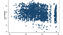
(a) Raw Scatter Plot

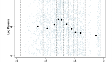
(b) Bin Cutoffs and Binscatter

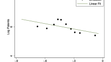
(c) Binscatter Plot

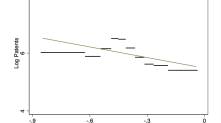
(d) Conditional Mean Point Est.

It is common practice to use additional control variables and fixed effects when constructing a binscatter. The standard plots, like Figure 1(c), will often be made after “controlling” for a set of covariates. This turns out to be a subtle issue, as the controls affect the visualization as well as the degree of uncertainty. Even the common practice of adding a regression line to a binned scatter plot is not straightforward to do correctly. We highlight important methodological and theoretical problems with the commonly used practice of first “residualizing out” additional covariates before constructing a binscatter. This is only formally justified when the true function is linear. Instead we show that the shape and support of the conditional mean can be incorrect when employing common practice. Figure 2 shows the practical importance of this issue by revisiting AGNS. Their benchmark specifications study the relation between log patents and marginal tax rates utilizing a rich set of control variables including fixed effects (see Table II and Figure I in AGNS). In their macro-level approach, the authors show that higher taxes negatively affect the quantity of innovation. Figure 2(a) is inspired by Figure I(A) in the original paper. Comparing the $x$ axis to the raw scatter plot of Figure 1(a) we see the distortion of the support. Figure 2(b) is the correctly scaled plot in the original paper; it is essentially uninformative about the shape of the mean. Finally, Figure 2(c) shows the corresponding results using our corrected covariate-adjustment approach.

Figure 2: Covariate Adjustment. This figure illustrates the role of covariate adjustment in the construction of binned scatter plots using data from Akcigit et al. (2022). The dependent variable is the log number of patents per state per year, and the independent variable is the log of the marginal net of tax rate for 90th percentile earners. The additional control variables are the lagged corporate tax rate, lagged population density, personal income per capita, and R&D tax credits, along with state and year fixed effects. The left plot is inspired by Figure I(A) in Akcigit et al. (2022) using 50, rather than 100, bins (when the corrected covariate adjustment is used there is insufficient variation in the variable of interest to feasibly accommodate the larger choice of bins). The middle plot is a correctly scaled version of the left plot. The right plot presents the binned scatter plot using the correct covariate adjustment approach. Binscatter estimates are based on weights of each state’s 1940 population count.

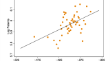
(a) Standard Binscatter
(Incorrect Scale)

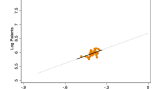
(b) Standard Binscatter
(Correct Scale)

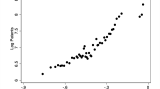
(c) Corrected Binscatter
(Correct Scale)

We provide an array of results and tools for binned scatter plots aimed at improving their empirical application. We improve on the estimation of conditional mean functions and provide tools for quantifying uncertainty. To facilitate our analysis, we first demonstrate that a binscatter is a nonparametric estimator, and we provide a modeling framework that enables formal analysis, allowing us to deliver new, more powerful methods and to resolve conceptual and implementation issues. We clarify precisely the parameters of interest in applications, both for visualization and formal inference. Our framework centers around a partially linear model, wherein we show how to control for additional variables in a principled and interpretable way, and discuss why prior implementations are not recommended.

Within our framework, we also discuss the choice of the number of bins, $J$. We elucidate how the choice of $J$ relates to the interpretation of the binscatter plot and its role in nonparametric estimation. When we use a binscatter to recover the conditional mean function we must assume $J$ grows with the sample size as is standard in semi- and nonparametric inference. In this case, we provide data-driven methods for an optimal choice of $J$. We can also consider a fixed, user-chosen $J$, which may yield a simple and appealing visualization of a coarsened version of the conditional mean. For example, selecting $J=10$ has a natural interpretation of comparing average outcomes in different deciles of the distribution of $x_{i}$. Our results also apply in this case.

We then turn to uncertainty quantification. For visualization, we provide confidence bands that capture the uncertainty in estimating the conditional mean or other functional parameters of interest. A confidence band is a region that contains the entire function with some pre-set probability, just as a confidence interval covers a single value, and is thus the proper tool for assessing uncertainty about the regression function. Confidence bands can be used to visually assess the plausibility of parametric functional forms, such as linearity. Confidence bands partly restore the uncertainty visualization capability of the classical scatter plot by capturing how certain we are about the functional form of the conditional mean. Further, our confidence bands are explicitly functions of the conditional heteroskedasticity in the underlying data. Delivering a valid confidence band requires novel theoretical results, which represent the main technical contribution of our work.

Figure 3(a) shows a confidence band for AGNS, relying on our data-drive choice of $J$ and robust bias correction methods to ensure the inference is valid. The binscatter itself is quite linear in appearance, in contrast with the original Figure 2(a). Moreover, Figure 3(b) shows that a linear function can be drawn within the confidence band (red line), so we can validly conclude that linearity is consistent with these data. In this case, our novel methods bolster the case for the paper’s original linear regression analysis. (In Section 5 we show an application where linearity is not supported, but our methods nonetheless reinforce an empirical conclusion and extend it in economically interesting ways.)

Figure 3: Confidence Bands. This figure illustrates uniform confidence bands using data from Akcigit et al. (2022). The dependent variable, independent variable, and controls are the same as in Figure 2. Binscatter estimates are based on weights of each state’s 1940 population count using the optimal number of bins as described in Section 3. Shaded regions denote 95% nominal confidence bands using a cluster-robust variance estimator with two-way clustering by year and state $\times$ five-year period.

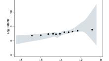
(a) Binscatter and Conf. Band

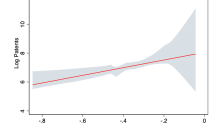
(b) Conf. Band

The paper proceeds as follows. We next briefly review the related literature and summarize our technical contributions. Section 2 formalizes binned scatter plots as a nonparametric estimator, including clarifying the parameter of interest and the correct method for adding control variables. Section 3 discusses the choice of the number of bins $J$. Section 4 studies uncertainty quantification for both visualization and testing. Throughout, we use the application of AGNS for illustration. In addition, Section 5 contains a second application, where we revisit Moretti (2021). Both applications highlight the usefulness of our results in empirical settings. Section 6 presents our main theoretical results and further discussion of the technical contributions of the paper. Finally, Section 7 concludes. An online Supplemental Appendix (SA hereafter) provides additional discussion and detail omitted from the main text, proofs of all our results, and a thorough account of our technical contributions. All of our methodological results are available in fully-featured Stata, R, and Python packages (see Cattaneo, Crump, Farrell and Feng (2023a) and https://nppackages.github.io/binsreg/).

1.1 Related Literature

Our paper fits into several literatures. Our work speaks most directly to the applied literature using binscatter methods, which is too large to enumerate here. Starr and Goldfarb (2020) gives an overview and many references. Beyond binscatter itself, binning has a long history in both visualization and formal estimation. The most familiar case is the classical histogram. Applying binning to regression problems dates back at least to the regressogram of Tukey (1961). The core idea has been applied in such diverse areas as climate studies, for nonlinearity detection (Schlenker and Roberts, 2009); program evaluation, called subclassification (Stuart, 2010); empirical finance, called portfolio sorting (Cattaneo et al., 2020b); and applied microeconomics, for visualization in bunching (Kleven, 2016) and regression discontinuity designs (Cattaneo and Titiunik, 2022).

In recent years, there has been related research looking at the importance and limitations of graphical analysis in different applied areas. For example, Korting et al. (2023) conducts a field experiment to investigate the role of visual inference and graphical representation in regression discontinuity designs via RD plots (Calonico et al., 2015). They conclude that unprincipled graphical methods could lead to misleading or incorrect empirical conclusions. Similar concerns regarding graphical analysis are raised by Freyaldenhoven et al. (2023) in the context of event study designs, where they proposed principled visualization methods. Graphical and visualization methods are also being actively discussed in the machine learning community (see Wang et al., 2021, and references therein, for an overview of the literature), where the importance of focusing on principled methods with well-understood properties for both in-sample and out-of-sample learning has been highlighted. Our paper contributes to this literature by offering principled approaches for visualization and inference employing binscatter methodology. Furthermore, well-executed visualization techniques can help with issues of statistical nonsignificance in empirical economics employing big data (Abadie, 2020).

Finally, our technical work contributes to the literature on nonparametric regression, particularly for uniform distributional approximations. Binning as a nonparametric procedure has been studied in the past, but existing theory is insufficient for our purposes for two main reasons. First, the extant literature cannot generally accommodate data-driven bin breakpoints, such as splitting the support by empirical quantiles. Such a choice of breakpoints generates random basis functions and so are not nested in previously obtained results on nonparametric series estimators. Second, where results are available, they imply overly stringent conditions on smoothing parameters ruling out simple averaging within each bin (which amounts to local constant fitting) and are thus not applicable to binscatter. Circumventing these limitations with new theoretical results is crucial to directly study the empirical practice of binned scatter plots.

Györfi et al. (2002) gives a textbook introduction to binning in nonparametric regression, where the procedure is known as partitioning regression. Recent work on partitioning, always assuming known breakpoints, includes convergence rates and pointwise distributional approximations (Ling and Hu, 2008; Cattaneo and Farrell, 2013), and uniform distributional approximations and robust bias correction methods (Cattaneo et al., 2020a). Partition regression is intimately linked to spline and wavelet methods, and the general results in our online SA treat these estimators as well, improving over earlier work by Shen et al. (1998), Huang (2003), Belloni et al. (2015), Cattaneo et al. (2020a), and references therein. We discuss these technical contributions in more detail in Section 6 and in the online SA.

2 Canonical Binscatter and Covariate Adjustments

The observed data is a random sample $(y_{i},x_{i},\mathbf{w}_{i}^{\prime})$, $i=1,2,\dots,n$, where $y_{i}$ is the outcome, $x_{i}$ is the main regressor of interest, and $\mathbf{w}_{i}$ are other covariates (e.g., pre-intervention characteristics or fixed effects). A binscatter has three key elements: the binning of the support of the covariate $x_{i}$, the estimation within each bin, and the way in which the controls $\mathbf{w}_{i}$ are handled. We discuss each of these in turn.

The partition of the support requires a choice of the number of bins, $J$, as well as how to divide the space. The choice of $J$ is the tuning parameter of this estimator, and in current practice it is often set independently of the data and equal to $J=10$ or $J=20$. We discuss the choice of $J$ in Section 3, but for now we take $J<n$ as given. For the spacing of the $J$ bins, we follow standard empirical practice and use the marginal empirical quantiles of $x_{i}$. Let $x_{(i)}$ denote the $i$-th order statistic of the sample $(x_{1},x_{2},\dots,x_{n})$ and $\lfloor\cdot\rfloor$ denote the floor operator. Then, the partitioning scheme is defined as $\widehat{\Delta}=\{\widehat{\mathcal{B}}_{1},\widehat{\mathcal{B}}_{2},\dots,\widehat{\mathcal{B}}_{J}\}$, where

$$\widehat{\mathcal{B}}_{j}=\begin{cases}\Big{[}x_{(1)},x_{(\lfloor n/J\rfloor)}\Big{)}&\qquad\text{if }j=1\\ \Big{[}x_{(\lfloor n(j-1)/J\rfloor)},x_{(\lfloor nj/J\rfloor)}\Big{)}&\qquad\text{if }j=2,3,\dots,J-1\\ \Big{[}x_{(\lfloor n(J-1)/J\rfloor)},x_{(n)}\Big{]}&\qquad\text{if }j=J\end{cases}.$$

Each estimated bin $\widehat{\mathcal{B}}_{j}$ contains (roughly) the same number of observations $N_{j}=\sum_{i=1}^{n}\mathds{1}_{\widehat{\mathcal{B}}_{j}}(x_{i})$, where $\mathds{1}_{\mathcal{A}}(x)=\mathds{1}(x\in\mathcal{A})$ is the indicator function. The notation $\widehat{\Delta}$ emphasizes that the partition is estimated from the data. Handling this randomness requires novel nonparametric statistical theory (Section 6). Our theory can accommodate quite general partitioning schemes, both random and nonrandom, provided high-level conditions are satisfied. In some cases the bins may be determined by the empirical application (e.g., income ranges, or schooling levels), while in others equally spaced bins may be more appropriate. However, given the ubiquity of quantile binning in economics, we focus on $\widehat{\Delta}$ as defined above.

We begin with the bivariate case, where there are no covariates $\mathbf{w}_{i}$. Given the partition $\widehat{\Delta}$, which encompasses a choice of the number of bins $J$, a binscatter is the collection of $J$ sample averages of the response variable: for each bin $\widehat{\mathcal{B}}_{j}$, we obtain $\bar{y}_{j}=\frac{1}{N_{j}}\sum_{i=1}^{n}\mathds{1}_{\widehat{\mathcal{B}}_{j}}(x_{i})y_{i}$; under our assumptions $\min_{1\leq j\leq J}N_{j}>0$ with probability approaching one in large samples. These sample averages are plotted as a “scatter” of points along with another, parametric estimate of the regression function $\upsilon_{0}(x_{i})=\mathbb{E}[y_{i}|x_{i}]$, often an ordinary least squares fit using the raw data. This construction is shown in Figures 1(b) and 1(c).

For fixed $J$, under regularity conditions, a binscatter can be interpreted as estimating $\xi_{0}(j)=\mathbb{E}[y_{i}|x_{i}\in\mathcal{B}_{j}]$, $j=1,2,\dots,J$, where $\mathcal{B}_{j}$ denotes the $j$th bin based on the population quantiles of $x_{i}$. This interpretation of the binscatter ignores the shape of the underlying conditional expectation within each bin, as it targets a likely misspecified constant model: $\xi_{0}(j)$ and $\upsilon_{0}(x)$ can be quite different for different values $x\in\mathcal{B}_{j}$, except in special cases. If $x_{i}$ was discrete with relatively few unique values, in which case binning would be unnecessary to begin with, or if the bins $\mathcal{B}_{1},\mathcal{B}_{2},\dots,\mathcal{B}_{J}$ had a natural economic interpretation (e.g., income ranges), then the $J$-dimensional parameter $\bm{\xi}_{0}=(\xi_{0}(1),\xi_{0}(2),\dots,\xi_{0}(J))^{\prime}$ could be of interest in applications. This parameter is intrinsically parametric in nature (for fixed $J$) and, as discussed below, all the results in the paper apply to $\bm{\xi}_{0}$ without modification.

When $x_{i}$ is continuously distributed or exhibits many distinct values, and the binning structure has no useful economic interpretation in and of itself, it is more natural to view the binscatter as a nonparametric approximation of $\upsilon_{0}(x)=\mathbb{E}[y_{i}|x_{i}]$ for appropriately chosen tuning parameter $J$. This approach characterizes misspecification errors (within and across bins) as well as nonparametric uncertainty in a principled way. Thus, we formalize a binscatter as a nonparametric estimator of $\upsilon_{0}(x)$ by recasting it as a piecewise constant fit: $\widehat{\upsilon}(x)=\bar{y}_{j}$ for all $x\in\widehat{\mathcal{B}}_{j}$, $j=1,2,\dots,J$. This is a least-squares series regression using a zero-degree piecewise polynomial. Formally, we define

$$\widehat{\upsilon}(x)=\widehat{\mathbf{b}}(x)^{\prime}\widehat{\bm{\xi}},\qquad\widehat{\bm{\xi}}=\operatorname*{arg\,min}_{\bm{\xi}\in\mathbb{R}^{J}}\sum_{i=1}^{n}(y_{i}-\widehat{\mathbf{b}}(x_{i})^{\prime}\bm{\xi})^{2},$$ (2.1)

where $\widehat{\mathbf{b}}(x)=[\mathds{1}_{\widehat{\mathcal{B}}_{1}}(x),\mathds{1}_{\widehat{\mathcal{B}}_{2}}(x),\cdots,\mathds{1}_{\widehat{\mathcal{B}}_{J}}(x)]^{\prime}$ is the binscatter basis given by a $J$-dimensional vector of orthogonal indicator variables, that is, the $j$-th component of $\widehat{\mathbf{b}}(x)$ records whether the evaluation point $x$ belongs to the $j$-th bin in the partition $\widehat{\Delta}$. This piecewise constant fit is shown in Figure 1(d), and from an econometric point of view, is identical to the dots of Figures 1(b) and 1(c). In the SA, we present results for a general polynomial fit within each bin, allowing for smoothness constraints across bins, which is useful to reduce misspecification bias.

2.1 Residualized Binscatter

We highlight an important methodological mistake with most applications of binscatter with covariates, including the Stata packages binscatter and binscatter2. Widespread empirical practice for covariate adjustment proceeds by first regressing out the covariates $\mathbf{w}_{i}$ from $x_{i}$ and $y_{i}$, and then applying the bivariate binscatter approach (2.1) to the residualized variables. This approach is heuristically motivated by the usual Frisch–Waugh–Lovell theorem for “regressing/partialling out” other covariates in linear regression settings.

From a nonparametric perspective, under regularity conditions, the residualized binscatter is consistent for

$$\mathbb{E}\big{[}y_{i}-\text{L}(y_{i}|\mathbf{w}_{i})\;\big{|}\;x_{i}-\text{L}(x_{i}|\mathbf{w}_{i})\big{]}$$ (2.2)

with $\text{L}(a_{i}|\mathbf{w}_{i})=(1,\mathbf{w}_{i}^{\prime})^{\prime}(\mathbb{E}[(1,\mathbf{w}_{i}^{\prime})^{\prime}(1,\mathbf{w}_{i}^{\prime})])^{-1}\mathbb{E}[(1,\mathbf{w}_{i}^{\prime})^{\prime}a_{i}]$, and thus $\text{L}(y_{i}|\mathbf{w}_{i})$ and $\text{L}(x_{i}|\mathbf{w}_{i})$ can be interpreted as the best (in mean square) linear approximations to, respectively, $\mathbb{E}[y_{i}|\mathbf{w}_{i}]$ and $\mathbb{E}[x_{i}|\mathbf{w}_{i}]$ (see Wooldridge, 2010, Chapter 2). $\text{L}(y_{i}|\mathbf{w}_{i})$ and $\text{L}(x_{i}|\mathbf{w}_{i})$ are, in general, misspecified approximations of the conditional expectations $\mathbb{E}[y_{i}|\mathbf{w}_{i}]$ and $\mathbb{E}[x_{i}|\mathbf{w}_{i}]$. Unless the true model is linear, the probability limit in (2.2) is difficult to interpret and does not align with standard economic reasoning. Furthermore, the shape of the function in (2.2) and even its support may be incorrect, and therefore can lead to incorrect empirical findings. The same problems arise when interpreting residualized binscatter from a fixed-$J$ perspective or when $x_{i}$ is discrete.

We therefore refer to the popular residualized binscatter method for covariate adjustment as incorrect or inconsistent for two main reasons. First, even when assuming a semi-linear conditional mean function $\mathbb{E}[y_{i}|x_{i},\mathbf{w}_{i}]=\mu_{0}(x_{i})+\mathbf{w}_{i}^{\prime}\bm{\gamma}_{0}$, residualized binscatter does not, in general, consistently estimate $\upsilon_{0}(x)$, $\mu_{0}(x)$, or $\mathbb{E}[y_{i}|x_{i}=x,\mathbf{w}_{i}=\mathbf{w}]$ for some evaluation point $\mathbf{w}$, despite being motivated by standard least squares methods. Only when $\mu_{0}(x)$ is linear does (2.2) reduce to $\mu_{0}(x)$, which need not equal $\upsilon_{0}(x)$ because $\mathbb{E}[y_{i}|x_{i}]=\mathbb{E}[\mathbb{E}[y_{i}|x_{i},\mathbf{w}_{i}]|x_{i}]=\mu_{0}(x_{i})+\mathbb{E}[\mathbf{w}_{i}|x_{i}]^{\prime}\bm{\gamma}_{0}$ under the semi-linear conditional mean structure. Therefore, from a point estimation and visualization perspective, residualized binscatter is not recommended for empirical work.

Second, from the perspective of assessing linearity or other shape features of the regression functions, the residualized binscatter is also not recommended. If $\mathbb{E}[y_{i}|x_{i},\mathbf{w}_{i}]=\mu_{0}(x_{i})+\mathbf{w}_{i}^{\prime}\bm{\gamma}_{0}$, with $\mu_{0}(x)$ a linear function of $x$, then the residualized binscatter plot will appear linear (for sufficiently large $n$ and an appropriate choice of $J$). However, linearity of the regression functions is only sufficient, not necessary: for some nonlinear $\mu_{0}(x_{i})$ the plot will appear linear, while for other nonlinear $\mu_{0}(x_{i})$ it will appear nonlinear. Thus, relying on residualized binscatter to assess linearity is not recommended because researchers may incorrectly conclude that $\mu_{0}(x_{i})$ (and hence $\mathbb{E}[y_{i}|x_{i},\mathbf{w}_{i}]=\mu_{0}(x_{i})+\mathbf{w}_{i}^{\prime}\bm{\gamma}_{0}$ for some value of $\mathbf{w}_{i}$) is linear from visual inspection or informal testing, thereby rendering subsequent empirical results based on a parametric linear regression potentially misleading.

Section SA-1.1 in the SA presents two simple parametric examples illustrating the potential biases introduced by residualized binscatter. The first example considers a Gaussian polynomial regression model, where $\mu_{0}(x)=x^{m}$ for some $m\in\mathbb{N}$, $d=1$, and $(y_{i},x_{i},w_{i})^{\prime}\thicksim\mathsf{Normal}$, and shows precisely how the different parameters underlying the model can change the shape of $\mu_{0}(x)$ as well as the concentration of $x_{i}-\text{L}(x_{i}|\mathbf{w}_{i})$, thereby affecting visually and formally the “shape” and “support” of (2.2). The second example considers $\mu_{0}(x)$ unrestricted, $d=1$, $w_{i}\thicksim\mathsf{Bernoulli}$, and $x_{i}|w_{i}=0\thicksim\mathsf{Uniform}$ and $x_{i}|w_{i}=1\thicksim\mathsf{Uniform}$ with disjoint supports, and shows how residualized binscatter can turn a nonlinear $\mu_{0}(x)$ into a linear function in (2.2) with incorrect support. These analytical examples complement our empirical applications (see Figure 2 and Figure 6), which illustrate with real data the detrimental effects of employing residualized binscatter for understanding the true form of the regression function relating the outcome $y_{i}$ to $x_{i}$ and $\mathbf{w}_{i}$.

2.2 Covariate-Adjusted Binscatter

With only bivariate data $(y_{i},x_{i})$, the binscatter (2.1) naturally provides (a visualization of) an estimate of the conditional mean function, $\upsilon_{0}(x_{i})=\mathbb{E}[y_{i}|x_{i}]$, which has a straightforward interpretation. Controlling for additional covariates complicates interpretation: we want to visually assess how $y_{i}$ and $x_{i}$ relate while “controlling” for $\mathbf{w}_{i}$ in some precise sense. There is not a universal answer to this problem, and the empirical literature employing binscatter methods is usually imprecise.

Motivated by (2.1), a more principled way to incorporate the covariates $\mathbf{w}_{i}$ into the binscatter is via semiparametric partially linear regression, as is commonly done in applied econometrics and program evaluation (Abadie and Cattaneo, 2018; Angrist and Pischke, 2008; Wooldridge, 2010). We define the covariate-adjusted binscatter as

$$\widehat{\mu}(x)=\widehat{\mathbf{b}}(x)^{\prime}\widehat{\bm{\beta}},\qquad\begin{bmatrix}\;\widehat{\bm{\beta}}\;\\ \;\widehat{\bm{\gamma}}\;\end{bmatrix}=\operatorname*{arg\,min}_{\bm{\beta}\in\mathbb{R}^{J},\bm{\gamma}\in\mathbb{R}^{d}}\sum_{i=1}^{n}(y_{i}-\widehat{\mathbf{b}}(x_{i})^{\prime}\bm{\beta}-\mathbf{w}_{i}^{\prime}\bm{\gamma})^{2}.$$ (2.3)

In this paper we take the semi-linear covariate-adjusted binscatter implementation (2.3) as the starting point of analysis, and thus view $\widehat{\Upsilon}(x_{i},\mathbf{w}_{i})=\widehat{\mu}(x_{i})+\mathbf{w}_{i}^{\prime}\widehat{\bm{\gamma}}$ as the plug-in estimator of

$$\mathbb{E}[y_{i}|x_{i},\mathbf{w}_{i}]=\mu_{0}(x_{i})+\mathbf{w}_{i}^{\prime}\bm{\gamma}_{0}=\Upsilon_{0}(x_{i},\mathbf{w}_{i}),$$ (2.4)

where we assume the usual identification restriction that $\mathbb{E}[\mathbb{V}[\mathbf{w}_{i}|x_{i}]]$ is positive definite. The imposed additive separability between $x_{i}$ and $\mathbf{w}_{i}$ of the conditional mean function follows standard empirical practice, but affects interpretation in certain cases. Our theoretical results continue to hold under misspecification of $\mathbb{E}[y_{i}|x_{i},\mathbf{w}_{i}]$, provided the probability limit of $\widehat{\Upsilon}(x_{i},\mathbf{w}_{i})$ is interpreted as a best mean square approximation of $\mathbb{E}[y_{i}|x_{i},\mathbf{w}_{i}]$ using functions of the form $g(x,\mathbf{w})=\mu(x)+\mathbf{w}^{\prime}\bm{\gamma}$. More precisely, under regularity conditions, the best mean square approximation would be $\text{P}(y_{i}|x_{i},\mathbf{w}_{i})=\mu^{\star}_{0}(x_{i})+\mathbf{w}_{i}^{\prime}\bm{\gamma}^{\star}_{0}$ with

$$\mu^{\star}_{0}(x_{i})=\mathbb{E}[y_{i}|x_{i}]-\mathbb{E}[\mathbf{w}_{i}|x_{i}]^{\prime}\bm{\gamma}^{\star}_{0}\qquad\text{and}\qquad\bm{\gamma}^{\star}_{0}=\big{(}\mathbb{E}\big{[}\mathbb{V}[\mathbf{w}_{i}|x_{i}]\big{]}\big{)}^{-1}\mathbb{E}\big{[}\mathbb{C}\mathrm{ov}[\mathbf{w}_{i},y_{i}|x_{i}]\big{]}.$$

In particular, $\mu^{\star}_{0}(x_{i})=\mu_{0}(x_{i})$ and $\bm{\gamma}^{\star}_{0}=\bm{\gamma}_{0}$ if (2.4) holds.

We adopt the semi-linear structure (2.4) throughout the paper because it is often invoked (explicitly or implicitly) for interpretation in empirical work. Cattaneo et al. (2023b) generalize binscatter methods to settings beyond the semi-linear conditional mean, including quantile regression, other nonlinear models such as logistic regression, and first-order interactions with a discrete covariate (e.g., a subgroup indicator). Those generalizations allow for a richer class of semiparametric parameters of interest and associated binscatter methods.

Given the working model (2.4), it remains to determine the (functional) parameter of interest. For visualization, a natural choice is a partial mean effect:

$$\Upsilon_{0}(x)=\Upsilon_{0}(x,\mathbb{E}[\mathbf{w}_{i}])=\mu_{0}(x)+\mathbb{E}[\mathbf{w}_{i}]^{\prime}\bm{\gamma}_{0},$$ (2.5)

which captures the average effect of $x_{i}$ on $y_{i}$ for units with covariates $\mathbf{w}_{i}$ at their average value $\mathbb{E}[\mathbf{w}_{i}]$, and thus gives an intuitive notion of the mean relationship of $x_{i}$ and $y_{i}$ after controlling for covariates $\mathbf{w}_{i}$ at their average values. The plug-in estimator is

$$\widehat{\Upsilon}(x)=\widehat{\mu}(x)+\bar{\mathbf{w}}^{\prime}\widehat{\bm{\gamma}}$$ (2.6)

with $\bar{\mathbf{w}}=\frac{1}{n}\sum_{i=1}^{n}\mathbf{w}_{i}$.

The structure imposed and the parameter considered are not innocuous, but lead to several advantages over other options. First, the target parameter in (2.5) has a natural partial mean interpretation because $\Upsilon_{0}(x)=\int\Upsilon_{0}(x,\mathbf{w})\text{d}F(\mathbf{w})=\mu_{0}(x_{i})+\mathbb{E}[\mathbf{w}_{i}]^{\prime}\bm{\gamma}_{0}$, where $F(\mathbf{w})=\mathbb{P}[\mathbf{w}_{i}\leq\mathbf{w}]$ is the marginal distribution function of the covariates. In addition, if $\mathbf{w}_{i}$ is mean independent of $x_{i}$, that is, if $\mathbb{E}[\mathbf{w}_{i}|x_{i}]=\mathbb{E}[\mathbf{w}_{i}]$, then $\upsilon_{0}(x_{i})=\mathbb{E}[y_{i}|x_{i}]=\mathbb{E}[\mathbb{E}[y_{i}|x_{i},\mathbf{w}_{i}]|x_{i}]=\mu_{0}(x_{i})+\mathbb{E}[\mathbf{w}_{i}|x_{i}]^{\prime}\bm{\gamma}_{0}=\Upsilon_{0}(x_{i})$. For example, if $x_{i}$ is a randomly assigned treatment dose and $\mathbf{w}_{i}$ are pre-intervention covariates, then $\Upsilon_{0}(x)$ corresponds to the dose-response average causal effect.

Second, $\Upsilon_{0}(x)$ matches the goal of examining potential nonlinearities (and other features) only along the $x_{i}$ dimension. The goal in a binscatter analysis is to control for $\mathbf{w}_{i}$, not to allow for (or discover) heterogeneity along these variables. This is why the covariates $\mathbf{w}_{i}$ are typically controlled for linearly, and without interactions with $x_{i}$, in the post-visualization regression analysis.

Third, $\Upsilon_{0}(x)$ has practical advantages. To see why, consider the alternative of estimating the fully-flexible conditional mean, $\mathbb{E}[y_{i}|x_{i},\mathbf{w}_{i}]$, and then integrating over the marginal distribution of $\mathbf{w}_{i}$. Although we would avoid imposing any structure on the conditional mean function, this approach would be impractical in common empirical settings as it would require nonparametric estimation in many dimensions. Taking the case of our running example to illustrate, AGNS control for four continuous variables, $49$ state fixed effects, and $60$ year fixed effects, so that $\dim(\mathbf{w}_{i})=113$. Furthermore, even when the partially linear model is adopted, there may still be a curse of dimensionality when interest lies in $\mu_{0}(x)$ because $\upsilon_{0}(x_{i})=\mu_{0}(x_{i})+\mathbb{E}[\mathbf{w}_{i}|x_{i}]^{\prime}\bm{\gamma}_{0}$, implying that the potentially high-dimensional conditional expectation $\mathbb{E}[\mathbf{w}_{i}|x_{i}]$ needs to be estimated. For example, in AGNS this would require fitting $113$ preliminary nonparametric regressions to estimate $\mathbb{E}[\mathbf{w}_{i}|x_{i}]$.

Finally, because $\Upsilon_{0}(x)$ is a special case of the more general partial mean $x\mapsto\Upsilon_{0}(x,\mathbf{w})=\mu_{0}(x)+\mathbf{w}^{\prime}\bm{\gamma}_{0}$ for some fixed value $\mathbf{w}$, it is possible to use other choices for the evaluation point $\mathbf{w}$. For example, setting the discrete components of $\mathbf{w}$ to a base category (such as zero) is a natural alternative. The choice of $\mathbf{w}$ will affect the interpretation of the estimand and the statistical properties of the estimator: see Section SA-1.2 in the SA for more discussion. In the remainder of the paper, we focus on $\Upsilon_{0}(x)$, but our theoretical results cover other choices of evaluation point $\mathbf{w}$ (see Section 6 and the SA).

Figure 2 in the Introduction showed how the results can change when using the correct and incorrect residualization (recall that panels (a) and (b) use the incorrect residualization). First, in Figure 2(a) the shape does not appear linear. Second, Figure 2(b) shows the extreme compression of the support of the estimate using the incorrect residualization by restoring the proper scale. This generally comes about because the variability of both the dependent and independent variables of interest have been overly suppressed. Finally, Panel (c) shows our estimator $\widehat{\Upsilon}(x)$ defined in (2.6), using the correct residualization (2.3). We can observe a much clearer shape of the estimate of the conditional expectation. In this case our methods give stronger visual support for the linear regression used by AGNS, in contrast to the apparent nonlinearity in the original binscatter. It is important to remember that although binscatters such as Figure 2 visually resemble conventional scatter plots of a data set, the plotted dots are actually a point estimate of a function (though in the case of Figure 2(a) and (b), not necessarily a useful function, see (2.2)).

We can also accommodate covariates in the fixed-$J$ case in a principled way. In this case, the estimator $\widehat{\Upsilon}(x)$ remains the same but the estimand, $\Upsilon_{0}(x)$, is replaced by its fixed-$J$ analogue: $\bm{\Xi}_{0}=(\Xi_{0}(1),\Xi_{0}(2),\dots,\Xi_{0}(J))^{\prime}$ with $\Xi_{0}(j)=\mathbf{b}(x)^{\prime}\bm{\beta}_{J}+\mathbb{E}[\mathbf{w}_{i}]^{\prime}\bm{\gamma}_{J}$ for $x\in\mathcal{B}_{j}$ with

$$\begin{bmatrix}\;\bm{\beta}_{J}\;\\ \;\bm{\gamma}_{J}\;\end{bmatrix}=\operatorname*{arg\,min}_{\bm{\beta}\in\mathbb{R}^{J},\bm{\gamma}\in\mathbb{R}^{d}}\mathbb{E}[(y_{i}-\mathbf{b}(x_{i})^{\prime}\bm{\beta}-\mathbf{w}_{i}^{\prime}\bm{\gamma})^{2}]$$

where $\mathbf{b}(x)=[\mathds{1}_{\mathcal{B}_{1}}(x),\mathds{1}_{\mathcal{B}_{2}}(x),\cdots,\mathds{1}_{\mathcal{B}_{J}}(x)]^{\prime}$. Under mild regularity conditions, as the number of bins increases, each bin becomes smaller and thus the fixed-$J$ parameter $\Xi_{0}(j)$ approximates $\Upsilon_{0}(x)$ for $x\in\mathcal{B}_{j}$ for all $j=1,2,\dots,J$ uniformly: $\max_{1\leq j\leq J}\sup_{x\in\mathcal{B}_{j}}|\Xi_{0}(j)-\Upsilon_{0}(x)|\to 0$ as $J\to\infty$. A small number of bins in finite samples, however, can make these parameters quite different due to misspecification errors induced by the local constant approximation within bins.

3 Choosing the Number of Bins

The final element of the binscatter estimator to formalize is the choice of $J$, the number of bins. It is common to encounter applications of binscatter where $J=\mathtt{J}$ for a fixed natural number $\mathtt{J}$, regardless of the data features. For example, the default in the Stata packages binscatter and binscatter2 is $\mathtt{J}=20$, while AGNS used $\mathtt{J}=100$. As already mentioned, from a fixed $J$ perspective, the canonical binscatter (2.1) estimates $\bm{\xi}_{0}$ and the covariate-adjusted binscatter (2.3) estimates $\bm{\Xi}_{0}$, neither of which may be the parameter of interest in a specific application. For example, the two parameters $\xi_{0}(j)=\mathbb{E}[y_{i}|x_{i}\in\mathcal{B}_{j}]$ and $\upsilon_{0}(x)$ for $x\in\mathcal{B}_{j}$ can lead to substantially different interpretations from both statistical and economic perspectives within bin $\mathcal{B}_{j}$. Furthermore, when comparing across bins, $(\xi_{0}(j):j=1,2,\dots,J)$ can be substantially different from $(\upsilon_{0}(x):x\in\mathcal{X})$. The choice of the tuning parameter $J$ determines the interpretation of the binscatter plot and estimand. In this section, we illustrate these concepts and discuss the choice of $J$ in practice.

We view binscatter as a sequence of approximating models indexed by $J$, where the larger $J$ (more bins) is, the less bias but more variance the estimator will exhibit. In other words, we view binscatter as most useful when the focus is on recovery of $\upsilon_{0}(x)$ or $\Upsilon_{0}(x)$, allowing us to visualize and conduct inference on those unknown functions. It is only by recovering $\upsilon_{0}(x)$ or $\Upsilon_{0}(x)$ that we can answer substantive questions regarding functional form or shape restrictions. In what is perhaps the leading case, if we wish to use a binscatter plot to precede a linear regression, then our interest is in whether $\upsilon_{0}(x)$ or $\Upsilon_{0}(x)$ is linear, so we must recover the true function. Recovering the coarsened version, as with a fixed $J=\mathtt{J}$, is not sufficient. The same reasoning applies to any statement regarding other shape constraints such as whether the relationship is monotonic or convex.

Consistent nonparametric estimation of $\upsilon_{0}(x)$ or $\Upsilon_{0}(x)$ requires $J$ to diverge with the sample size, but neither too rapidly nor too slowly. To remove the approximation bias, a sufficiently large $J$ is required to overcome the limited flexibility of the constant fit within bins: intuitively, as $J$ diverges, the bin width collapses, and $\xi_{0}(j)=\mathbb{E}[y_{i}|x_{i}\in\mathcal{B}_{j}]\approx\upsilon_{0}(x)$ for $x\in\mathcal{B}_{j}$ because the width of the bin $\mathcal{B}_{j}$ shrinks as $J$ increases. However, the variance of the estimator increases with $J$ because variance is controlled by the bin-specific sample sizes, which are roughly $n/J$. Thus, as is familiar in nonparametric estimation, we face a bias-variance trade-off when choosing $J$. Figure 4 illustrates this bias-variance trade-off in our running application. In Panel (a) we use $\mathtt{J}=5$. If we consider this choice as fixed, we can use these results to, for example, compare the productivity of those subject to the highest quintile of all tax rates on high earners to those in areas where taxes on high earners are in the lowest quintile. But for the purpose of nonparametric estimation and inference, the estimator is oversmoothed: the number of bins is too small to remove sufficient bias. At the other extreme, Panel (c) uses 50 bins, and the estimator is undersmoothed (too wiggly) to provide a reliable visualization of the conditional mean.

Figure 4: Choice of $J$. This figure illustrates the role of the choice of $J$ using data from Akcigit et al. (2022). The dependent variable, independent variable, and controls are the same as in Figure 2. The left and right plots show a binned scatter plot with $J=5$ and $J=50$, respectively. The middle plot shows the binned scatter plot using the optimal choice of $J=11$ based on a cluster-robust variance estimator with two-way clustering by year and state $\times$ five-year period. Binscatter estimates are based on weights of each state’s 1940 population count.

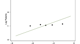
(a) Oversmoothed

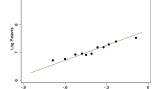
(b) Optimal

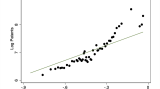
(c) Undersmoothed

A wide range of choices for $J$ will, in large sample theory, ensure that both bias and variance are adequately controlled and thus yield a consistent estimator and valid distributional approximation. However, such rate restrictions are not informative enough to guide practice. It is therefore important to have tight guidance for empirical research. To accomplish this, we develop a selector for $J$ that is optimal in terms of integrated mean square error (IMSE). As is standard in nonparametrics, the IMSE-optimal $J$ balances variance and (squared) bias, resulting in

$$J_{\mathtt{IMSE}}=\left\lceil\left(\frac{2\mathscr{B}_{n}}{\mathscr{V}_{n}}\right)^{1/3}\;n^{1/3}\right\rceil,$$ (3.1)

The terms $\mathscr{V}_{n}$ and $\mathscr{B}_{n}$ capture the asymptotic variance and (squared) bias of the binscatter, respectively. We give complete expressions in the SA. All that matters at present is that (i) both are generally bounded and bounded away from zero under minimal assumptions, (ii) the variance accounts for heteroskedasticity and clustering, and (iii) both incorporate the additional covariates appropriately, so that the optimal $J$ depends on the presence of $\mathbf{w}_{i}$. A formal IMSE expansion is discussed in Section 6 and given in Theorem SA-3.4 in the SA, along with a uniform consistency result in Corollary SA-3.1, which has the same rate up to a $\log(J)$ factor. A feasible version, $\widehat{J}_{\mathtt{IMSE}}$, is straightforward to implement. Details are given in Section SA-4 in the SA.

The formula for $J_{\mathtt{IMSE}}$ intuitively reflects the trade-off as depicted in Figure 4. If the data are highly variable $\mathscr{V}_{n}$ will be large, driving down $J_{\mathtt{IMSE}}$, so that each bin has a large sample size. On the other hand, if $\mu_{0}(x)$ is highly nonsmooth, $\mathscr{B}_{n}$ will be large, and more bins are required to adequately remove bias. Figure 4(b) shows our feasible IMSE-optimal choice in the data of AGNS, where we find $\widehat{J}_{\mathtt{IMSE}}=11$. With this choice, we obtain a visualization and optimal nonparametric estimation of $\mu_{0}(x)$ and $\Upsilon_{0}(x)$. We will also base our uncertainty visualization and quantification around this implementation, to ensure validity, as we detail in the next section.

Even if a fixed $J=\mathtt{J}$ is chosen for an application, the data-driven choice $\widehat{J}_{\mathtt{IMSE}}$ can provide a useful benchmark to understand better the bias-variance trade-off underlying the binscatter implementation. For example, choosing a $\mathtt{J}$ that is much larger than $\widehat{J}_{\mathtt{IMSE}}$ will yield a binscatter that is likely to exhibit considerably more variability than bias, given the data generating process. Thus, the data-driven choice $\widehat{J}_{\mathtt{IMSE}}$ can help applied researchers discipline and improve their fixed $J=\mathtt{J}$ binscatter implementations.

In the remainder of the paper we focus on the covariate-adjusted binscatter estimate (2.6) implemented using $J_{\mathtt{IMSE}}$, or its fixed-$J$ analogue when appropriate for concreteness. Our technical results in the SA accommodate other choices of $J$ as a function of the sample size with and without covariate-adjustment, thereby covering, in particular, the canonical binscatter estimate (2.1) implemented using its corresponding $J_{\mathtt{IMSE}}$. See Section 6 for a brief overview.

4 Quantifying Uncertainty

We provide both visualization and analytical tools to capture the uncertainty underlying the mean estimate $\widehat{\Upsilon}(x)=\widehat{\mu}(x)+\bar{\mathbf{w}}^{\prime}\widehat{\bm{\gamma}}$, valid simultaneously for all values of $x\in\mathcal{X}$. This uniformity over $x\in\mathcal{X}$ is required both to answer the substantive questions of interest in empirical work and to provide a correct visualization of the uncertainty for the function $\Upsilon_{0}(x)$. Uniform inference theory is a major technical contribution of this paper (see Section 6 and the SA). Confidence bands directly enhance the visualization capabilities of binned scatter plots by summarizing and displaying the uncertainty around the estimate $\widehat{\Upsilon}(x)$. Loosely speaking, a confidence band is simply a confidence “interval” for a function, and is interpreted much like a traditional confidence interval.

A typical confidence interval for a single parameter (such as a mean or regression coefficient) is a range between two endpoint values that, in repeated samples, covers the true parameter with a prespecified probability. The width of a confidence interval increases with the uncertainty in the data. Intuitively, the interval shows the values of the parameter that are compatible with the data. For example, if the interval contains zero, then zero is a plausible value for the true parameter. That is, the null hypothesis of zero cannot be rejected.

A confidence band is essentially the same, but as a function of $x$, and can therefore be directly plotted. It is the area between two endpoint functions that contains all the functions $\Upsilon_{0}(x)$ that are compatible with the data for some pre-set probability. Matching the use of a confidence interval, the band can be used to evaluate hypotheses. For example, if the band contains a linear function, then linearity is a plausible form for $\mu_{0}(x)$ (as in Figure 3(b)). That is, the null hypothesis that $x$ enters $\Upsilon_{0}(x)$ linearly cannot be rejected. The same logic can be used for other shape restrictions: if the band contains monotonic functions, then monotonicity of $\Upsilon_{0}(x)$ is consistent with the data. This is illustrated below. Thus, adding a confidence band is an important step in any binscatter, to visually assess and communicate the uncertainty, just as the addition of standard errors is an important step and good empirical practice in any regression analysis. The reader can see not only the estimate of the relationship (the “dots” of the binscatter), but also the uncertainty surrounding this estimate.

The construction and theory of our confidence bands also intuitively match standard confidence intervals. First, our confidence bands reflect the underlying heteroskedastic variance in the data uniformly over the support of $x_{i}$. While the visualizations do reflect these quantities, they are not directly shown or formally accounted for. This is analogous to how a simple confidence interval for the mean reflects only estimation uncertainty about the parameter, even though the interval depends on the variance of the data. For visualizing the “spread” and detecting outliers conditional quantiles may be more useful (see Cattaneo et al., 2023b). Second, the upper/lower endpoint functions are given by the point estimate plus/minus a critical value times a standard error. In this way, the width of the band at any point depends on the overall uncertainty and the heteroskedasticity.

Before presenting the confidence band formulation, we must be precise about the object we intend to cover with the confidence band. If $J$ is taken as fixed, the parameter is $\bm{\Xi}_{0}$, and inference is parametric because there is no misspecification bias for that parameter. However, as explained before, in many applications the parameter of interest will not be $\bm{\Xi}_{0}$ but rather $\Upsilon_{0}(x)$, leading to unavoidable misspecification errors introduced by the binscatter approximation to the true function. Thus, we focus on a band to cover the function $\Upsilon_{0}(x)$ given in (2.5). It is only in this case that the band can be used to assess properties of the function of interest. Testing linearity (prior to a regression analysis) is the most common use case, but binned scatter plots are also utilized to assess other shape restrictions (see, for example, Shapiro and Wilson (2021) or Feigenberg and Miller (2021)). Regardless of the application, the band must be constructed from a nonparametric perspective (i.e., assuming $J$ diverging to account explicitly for misspecification error).

To ensure validity of the nonparametric confidence band, we will use $J_{\mathtt{IMSE}}$ given in (3.1) together with debiasing to remove the first-order nonparametric misspecification bias introduced by employing the IMSE-optimal binscatter. More specifically, we employ a simple application of the standard robust bias correction method for debiasing (Calonico et al., 2018; Cattaneo et al., 2020a; Calonico et al., 2022). Section 6 discusses the theoretical foundations, and the SA provides all the details, while here we describe the key ideas heuristically. The confidence band for $\Upsilon_{0}(x)$ is

$$\widehat{I}_{\tt RBC}(x)=\Big{[}\;\widehat{\Upsilon}_{\tt BC}(x)\pm\mathfrak{c}_{\tt RBC}\cdot\sqrt{\widehat{\Omega}_{\tt RBC}(x)/n}\;\Big{]},$$ (4.1)

where $\widehat{\Upsilon}_{\tt BC}(x)$ denotes the covariate-adjusted debiased binscatter estimator of $\Upsilon_{0}(x)$, $\widehat{\Omega}_{\tt RBC}(x)/n$ is its variance estimator, and $\mathfrak{c}_{\tt RBC}$ is the appropriate quantile to make the confidence band uniformly valid. The exact formulas are given in Section 6. Intuitively, $\widehat{\Upsilon}_{\tt BC}(x)=\widehat{\Upsilon}(x)-\widehat{\textsf{Bias}}[\widehat{\Upsilon}(x)]$, where $\widehat{\textsf{Bias}}[\widehat{\Upsilon}(x)]$ denotes the bias correction, and $\widehat{\Omega}_{\tt RBC}(x)/n=\widehat{\textsf{Var}}[\widehat{\Upsilon}_{\tt BC}(x)]$ is an estimator of the variance of $\widehat{\Upsilon}_{\tt BC}(x)$ not just of $\widehat{\Upsilon}(x)$. The key idea underlying the robust bias correction method is that debiasing introduces additional estimation uncertainty that must be incorporated explicitly into the standard error formula. While there are many ways of debiasing the IMSE-optimal point estimator $\widehat{\Upsilon}(x)$, a simple one proceeds by fitting a constrained linear regression within each bin where the estimated coefficients are restricted to ensure that the binscatter estimator is continuous; that is, the constraints force the piecewise linear fits within bins to be connected at the boundary of the bins. This construction ensures that the associated confidence bands are also continuous. More details are given in Section 6 and in the SA.

Our results rely on standard regularity conditions for valid uniform distribution theory with robust bias correction discussed in Section 6, and the SA gives results under more general, and in some cases weaker, conditions. More precisely, for $\alpha\in(0,1)$, we show that

$$\mathbb{P}\Big{[}\Upsilon_{0}(x)\in\widehat{I}_{\tt RBC}(x),\;\text{for all }x\in\mathcal{X}\Big{]}\to 1-\alpha$$ (4.2)

giving formal validity, that is, in repeated samples the area covers the true function $\Upsilon_{0}(x)$ with a pre-specified probability $1-\alpha$. Recall that $\Upsilon_{0}(x)$, by definition, uses the mean of $\mathbf{w}_{i}$; other possible choices and their impact on the confidence band are discussed in Section SA-1.2 of the SA.

The result in (4.2) shows how to add valid confidence bands to any binned scatter plot. This visual assessment of uncertainty is an important step in any analysis. Our discussion focused on the nonparametric uncertainty quantification when employing the IMSE-optimal binscatter constructed using $J=J_{\mathtt{IMSE}}$ bins and debiasing using within-bin linear regression, but our theoretical results remain valid more generally for other choices of $J$ and debiasing approaches. Furthermore, the bands continue to be valid when $J=\mathtt{J}$ is fixed provided the estimand $\Upsilon_{0}(x)$ is switched to its fixed-$J$ analogue $\bm{\Xi}_{0}$. In this latter case, robust bias correction is not technically needed because the misspecification error is removed by assumption (i.e., by redefining the parameter of interest).

If $x_{i}$ is discrete, or the researcher is content with the coarsened version of the parameter $\bm{\Xi}_{0}$ under a fixed-$J$ approach, our results provide (uniformly) valid inference for the covariate-adjusted outcome mean conditional on falling in each bin. This amounts to adding pointwise confidence intervals to a plot – which is common practice in many uses – and making corrections for multiple testing. These can be used directly to assess uncertainty about the mean for a masspoint of $x_{i}$ (or within a given quantile range), but cannot be used to assess functional features of the regression function $\Upsilon_{0}(x)$ as a whole.

Figure 5 compares these two cases, fixed-$J$ versus large-$J$, using the data of AGNS. Figure 5(a) shows confidence bands for $\mathtt{J}=5$, with the interpretation of studying the conditional expectation of log patents given marginal tax rates in a specific quintile controlling for additional covariates (i.e., $\bm{\Xi}_{0}$). As we saw in Figure 4(a), the point estimates are all relatively similar across quintiles and, in fact, we cannot rule out that all five conditional means are the same. This can be gleaned by the dashed horizontal line in Figure 5(a) which comfortably sits in all five shaded regions. In Figure 5(b) we consider inference on $\Upsilon_{0}(x)$ using the optimal choice of $J$ (as in Figures 3 and 4(b)). We have already discussed that the confidence band is consistent with a linear relation between the variables. However, we can also highlight classes of functions that the confidence band excludes. The dashed horizontal line is set to the upper bound of the confidence band at the smallest value of $x$ in the support. We can immediately observe that the confidence band rules out any horizontal lines, i.e., we can reject that log patents have no relationship with marginal tax rates. This horizontal line is also a useful visual cue to evaluate the class of monotonically decreasing functions. Clearly, we can also reject a monotonically decreasing relation between the two variables. Figure 5 illustrates that the use of confidence bands for investigating the attributes of the true functional form is simple and straightforward.

Figure 5: Quantifying Uncertainty: The Role of $J$. This figure illustrates uniform confidence bands using data from Akcigit et al. (2022). The dependent variable, independent variable, and controls are the same as in Figure 2. The left plot presents a confidence band for $\bm{\Xi}_{0}$ whereas the right plot shows the confidence band for $\Upsilon_{0}(x)$. Binscatter estimates are based on weights of each state’s 1940 population count. Shaded regions denote 95% nominal confidence bands using a cluster-robust variance estimator with two-way clustering by year and state $\times$ five-year period.

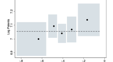
(a) Fixed $J$

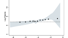
(b) Diverging $J$

In addition to employing confidence bands for testing substantive hypotheses about $\Upsilon_{0}(x)$ such as positivity, monotonicity, or concavity, we develop formal hypothesis testing based on canonical binscatter methods in the SA for completeness. These methods are also available in our companion software implementations (Cattaneo et al., 2023a), and can be used to complement the empirical analysis based on canonical binscatter discussed previously, offering potential power improvements as well as more precise econometric conclusions (e.g., formal p-values). Since using the confidence bands for testing is already a valid, easy, and intuitive econometric methodology for empirical work employing canonical binscatter, we offer further technical discussion of the companion formal hypothesis testing methods for parametric specification and shape restrictions in Cattaneo et al. (2023b), covering generalized binscatter methods based on both least squares and other loss functions (e.g., quantile or logistic regression).

5 Another Empirical Illustration

As an additional empirical application we revisit Moretti (2021), which examined the relation between the productivity of top inventors and high-tech clusters, where clusters are defined as activity in a city of a specific research field (e.g., computer scientists in Silicon Valley). The paper estimates an elasticity of number of patents in a year with respect to cluster size of 0.0676. The statistically significant positive relationship aligns with the empirical observation that increasingly large subsidies are being offered by states and localities for high-tech firms to relocate within their regions.

We begin our analysis with a raw scatter plot of the data (top left of Figure 6). With close to one million observations, the scatter plot is both dense and uninformative. In the top right plot we replicate Figure 4 in Moretti (2021) which is a binned scatter plot controlling for year, research field, and city effects. It is intuitive to view and interpret this figure as one would a conventional scatter plot – a cloud of points with a regression line fit to the “data” – and we would conclude that there may be a positive but noisy relationship between these two variables. This interpretation is tempting, and indeed the very name “binscatter” invites this, but as previously discussed it is incorrect: the dots here are not data points but estimates of the conditional mean function.

This is emphasized in Figure 6(c) which is the implied estimate of the conditional mean function. This plot is formally identical to the figure in the original paper (Figure 6(b)), but visually very different; moreover, assuming that the wiggly step function is well-approximated by a line seems inappropriate. However, there are two issues here: the incorrect residualization has been performed and the number of bins is too large, leading to substantial undersmoothing. Figure 6(d) addresses the former issue, applying our corrected approach to covariates overlaying the incorrectly residualized version now at the correct scale, making the difference starker. Correctly adjusting for covariates presents a much clearer picture of the empirical conclusions to be drawn from the data than do Figures 6(b) and 6(c).

This visual pattern is even more apparent in the bottom left plot where we utilize the IMSE-optimal choice of $J$ ($J_{\mathtt{IMSE}}=18$). Now, the point estimate of the conditional expectation function is thrown into sharper relief. For smaller cluster sizes, the conditional expectation appears roughly flat whereas for larger cluster sizes, the estimate rises sharply. This gives the appearance of a nonlinear relation between productivity and high-tech clusters. We can formalize this conclusion by utilizing the associated confidence band also shown in Figure 6(e). We clearly reject the null of no relationship between the variables as the confidence band does not contain a horizontal line. Furthermore, we can also clearly reject linearity as no linear function can be wholly enveloped by the confidence band. However, we fail to reject convexity given the shape of the confidence band. Taken in sum, these results suggest a nonlinear relation between the number of patents and cluster size. Figure 6(f) replicates this analysis for the main specification in Moretti (2021, Table 3, Columnn (8)) which includes 11 different fixed effects. We draw the same conclusions, with strong evidence against a linear functional form. This added nuance to the results of Moretti (2021) obtained through our new tools is not inconsequential. Taken at face value, it would imply that states and localities which have only small clusters of inventors might have to offer very generous incentives in order to grow their cluster size sufficiently large to generate the positive agglomeration effects presented in Moretti (2021).

Figure 6: Relation Between Productivity of Top Inventors and High-Tech Clusters. This figure uses the data from Moretti (2021). The dependent variable is the log number of patents per inventor per year, and the independent variable is the log cluster size. The top left plot shows a raw scatter plot of the data. The top right plot replicates Figure 4 in Moretti (2021) which controls for year, research field, and city effects while the middle left plot shows the implied estimated conditional mean function (2.2). The incorrect residualization versus the semi-linear specification introduced in Section 2 (both for 40 bins) is shown in the middle right chart. The bottom left chart uses the optimal choice of $J$ introduced in Section 3. The bottom right chart again uses the optimal choice of $J$ but for the main specification of Moretti (2021, Table 3, Columnn (8)). Shaded regions denote 95% confidence bands using a cluster-robust variance estimator with clustering by city $\times$ field.

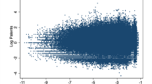
(a) Raw Scatter plot

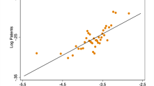
(b) Fig. 4 of Moretti (2021)

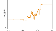
(c) Incorrect Residualization

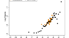
(d) Covariate Adjustment

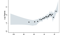
(e) Confidence Band

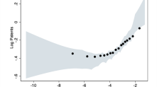
(f) Confidence Band (Full Specification)

6 Theoretical Foundations

The SA reports our novel theoretical results for partitioning-based estimators with semi-linear covariate-adjustment and random binning based on empirical quantiles, which provide all the necessary econometric tools to formally study canonical and covariate-adjusted binscatter least squares methods. This section overviews those results, and discusses them in connection with the previous sections.

We study a covariate-adjusted estimator with more flexible basis functions allowing for polynomial fitting within bins and smoothness constraints across bins. The $p$-th order polynomial, $(s-1)$-times continuously differentiable, covariate-adjusted extended binscatter estimator is

$$\widehat{\mu}^{(v)}(x)=\widehat{\mathbf{b}}_{p,s}^{(v)}(x)^{\prime}\widehat{\bm{\beta}},\qquad\begin{bmatrix}\;\widehat{\bm{\beta}}\;\\ \;\widehat{\bm{\gamma}}\;\end{bmatrix}=\operatorname*{arg\,min}_{\bm{\beta},\bm{\gamma}}\sum_{i=1}^{n}(y_{i}-\widehat{\mathbf{b}}_{p,s}(x_{i})^{\prime}\bm{\beta}-\mathbf{w}_{i}^{\prime}\bm{\gamma})^{2},\qquad 0\leq v,s\leq p.$$ (6.1)

where $\widehat{\mathbf{b}}_{p,s}(x)=\widehat{\mathbf{T}}_{s}[\widehat{\mathbf{b}}(x)\otimes(1,x,\dots,x^{p})^{\prime}]$, $\widehat{\mathbf{T}}_{s}$ is a $[(p+1)J-(J-1)s]\times(p+1)J$ matrix of linear restrictions ensuring that the $(s-1)$-th derivative of the estimate is continuous, $\otimes$ denotes the Kronecker product, and $g^{(v)}(x)=\frac{\text{d}^{v}}{\text{d}x^{v}}g(x)$. (See Section SA-2 for further details.) For example, $s=1$ returns a continuous but nondifferentiable function ($\widehat{\mathbf{T}}_{1}$ constrains the polynomial fits within bins to be connected at the boundary of the bins), while $s=0$ gives a discontinuous function ($\widehat{\mathbf{T}}_{0}$ is the identity matrix). The form of $\widehat{\mathbf{T}}_{s}$ is given in the SA, and it depends on the estimated quantiles. If $p=0$ (forcing $s=v=0$), then (6.1) reduces to (2.3) because $\widehat{\mathbf{b}}_{0,0}(x)=\widehat{\mathbf{b}}(x)$ which is equivalent to the Haar basis or a zero-degree spline. The additional generality of allowing for polynomial basis functions, beyond piecewise constant functions, is useful for estimating derivatives of the function of interest ($v>0$), as well as for reducing the smoothing bias of the estimator. The SA treats the general case $0\leq v,s\leq p$, but in the paper we only consider $s=p$, with $p=0$ for binscatter estimation and $p\geq 1$ for inference, and thus we set $\widehat{\mathbf{b}}_{p}(x)=\widehat{\mathbf{b}}_{p,p}(x)$ to simplify notation (and note that $\widehat{\mathbf{b}}(x)=\widehat{\mathbf{b}}_{0}(x)=\widehat{\mathbf{b}}_{0,0}(x)$). More specifically, the implementations of robust bias correction discussed in Section 4 sets $(p,s,v)=(1,1,0)$.

The following assumption gives a simplified version of the conditions imposed in the SA.

Assumption 1.

The sample $(y_{i},x_{i},\mathbf{w}_{i}^{\prime})$, $i=1,2,\dots,n$, is i.i.d. and satisfies (2.4). The functions $\mu_{0}(x)$ and $\mathbb{E}[\mathbf{w}_{i}|x_{i}=x]$ are $(p+2)$-times continuously differentiable. The covariate $x_{i}$ has a Lipschitz continuous density function $f_{X}(x)$ bounded away from zero on the compact support $\mathcal{X}$. The minimum eigenvalue of $\mathbb{V}[\mathbf{w}_{i}|x_{i}=x]$ is uniformly bounded away from zero. For $\epsilon_{i}=y_{i}-\mu_{0}(x_{i})-\mathbf{w}_{i}^{\prime}\bm{\gamma}_{0}$, $\sigma^{2}(x)=\mathbb{E}[\epsilon_{i}^{2}|x_{i}=x]$ is Lipschitz continuous and bounded away from zero, and $\mathbb{E}[\|\mathbf{w}_{i}\|^{4}|x_{i}=x]$, $\mathbb{E}[\epsilon_{i}^{4}|x_{i}=x]$, and $\mathbb{E}[\epsilon_{i}^{2}|x_{i}=x,\mathbf{w}_{i}=\mathbf{w}]$ are uniformly bounded, where $\|\cdot\|$ is the Euclidean norm.

Section SA-3.1 presents new technical lemmas for random partitions based on empirical quantiles. Those results include general characterizations of the “regularity” of the random partitioning scheme (Lemmas SA-3.1 and SA-3.2) and of the associated random basis functions (Lemmas SA-3.3 and SA-3.4). These results give sharp control on the underlying random binning scheme of binscatter methods.

Sections SA-3.2–SA-3.7 study large sample point estimation and distributional properties of the extended covariate-adjusted binscatter estimator. Preliminary technical results include: (i) technical lemmas for the Gram matrix (Lemma SA-3.5), asymptotic variance (Lemmas SA-3.6 and SA-3.7), approximation error (Lemma SA-3.8), and covariate adjustments (Lemma SA-3.9); (ii) stochastic linearization and uniform convergence rates (Theorem SA-3.1 and Corollary SA-3.1) and variance estimation (Theorem SA-3.2); and (iii) pointwise distributional approximation (Theorem SA-3.3). All these results explicitly account for the random binning scheme.

Using our new technical results, Section SA-3.5 also establishes a density-weighted IMSE expansion of the binscatter estimator (Theorem SA-3.4). Letting $\mathsf{IMSE}[\widehat{\Upsilon}^{(v)}]=\int\mathbb{E}[(\widehat{\Upsilon}^{(v)}(x)-\Upsilon^{(v)}_{0}(x))^{2}|x_{1},\dots,x_{n},\mathbf{w}_{1},\dots,\mathbf{w}_{n}]f_{X}(x)dx$, a simplified version of our general result follows.

Theorem 1 (IMSE).

Let Assumption 1 hold, $0\leq v\leq p$, $J\log(J)/n\to 0$, and $nJ^{-4p-5}\to 0$. Then, $\mathsf{IMSE}[\widehat{\Upsilon}^{(v)}]=\frac{J^{1+2v}}{n}\mathscr{V}_{n}(p,s,v)+J^{-2(p+1-v)}\mathscr{B}_{n}(p,s,v)+o_{\mathbb{P}}(\frac{J^{1+2v}}{n}+J^{-2(p+1-v)})$, where $\mathscr{V}_{n}(p,s,v)$ and $\mathscr{B}_{n}(p,s,v)$ are non-random, $n$-varying bounded sequences (see Section SA-3.5).

Optimizing the leading terms over $J$ gives the optimal choice $J_{\mathtt{IMSE}}(p,s,v)$, and specializing it to $p=s=v=0$ gives (3.1). Feasible IMSE-optimal tuning parameter selection is discussed in Section SA-4. All these results explicitly account for the random binning scheme and the covariate adjustment.

Section SA-3.6 reports our most noteworthy novel technical result: a conditional strong approximation for the extended binscatter estimator, which circumvents a fundamental lack of uniformity of the random binning basis $\widehat{\mathbf{b}}_{p}(x)$, while still delivering a sufficiently fast uniform coupling, requiring only $J^{2}/n\to 0$ (up to $\log(n)$ terms). In fact, if a subexponential moment restriction holds for $\epsilon_{i}$, it suffices that $J/n\rightarrow 0$ (up to $\log(n)$ terms). Our rate conditions not only improve on previous results in the literature, but also allow for canonical binscatter (i.e., there exists a sequence $J\to\infty$ such that bias and variance are simultaneously controlled even when $p=s=0$).

The starting point is the Studentized $t$-statistic that centers and scales the extended binscatter estimator $\widehat{\Upsilon}^{(v)}(x)=\widehat{\mu}^{(v)}(x)+\mathds{1}(v=0)\bar{\mathbf{w}}^{\prime}\widehat{\bm{\gamma}}$ of the extended parameter of interest $\Upsilon_{0}^{(v)}(x)=\mu_{0}^{(v)}(x)+\mathds{1}(v=0)\mathbb{E}[\mathbf{w}_{i}]^{\prime}\bm{\gamma}_{0}$. We index important objects with $p$ (recall that $s=p$ in the paper, but the SA treats the general case). We study the $t$-statistic

$$T_{p}(x)=\frac{\widehat{\Upsilon}^{(v)}(x)-\Upsilon^{(v)}_{0}(x)}{\sqrt{\widehat{\Omega}(x)/n}},$$

where $\widehat{\Omega}(x)=\widehat{\mathbf{b}}_{p}^{(v)}(x)^{\prime}\widehat{\mathbf{Q}}^{-1}\widehat{\bm{\Sigma}}\widehat{\mathbf{Q}}^{-1}\widehat{\mathbf{b}}^{(v)}_{p}(x)$, $\widehat{\mathbf{Q}}=\frac{1}{n}\sum_{i=1}^{n}\widehat{\mathbf{b}}_{p}(x_{i})\widehat{\mathbf{b}}_{p}(x_{i})^{\prime}$, and $\widehat{\bm{\Sigma}}=\frac{1}{n}\sum_{i=1}^{n}\widehat{\mathbf{b}}_{p}(x_{i})\widehat{\mathbf{b}}_{p}(x_{i})^{\prime}(y_{i}-\widehat{\mathbf{b}}_{p}(x_{i})^{\prime}\widehat{\bm{\beta}}-\mathbf{w}_{i}^{\prime}\widehat{\bm{\gamma}})^{2}$. We seek a distributional approximation for the entire stochastic process $(T_{p}(x):x\in\mathcal{X})$ because this allows us to study the visualization and econometric properties of the entire binscatter fit $(\widehat{\Upsilon}^{(v)}(x):x\in\mathcal{X})$ simultaneously. Using this strong approximation we can compute the critical values for valid confidence bands and hypothesis testing. Our approach gives a simple, tractable method for computing critical values based on random draws from the Gaussian distribution.

The randomness of the partition $\widehat{\Delta}$ (which is inherited by the basis functions themselves) is not just ruled out by the assumptions of prior work, but rather it is not even possible to obtain a valid strong approximation for the entire stochastic process $(T_{p}(x):x\in\mathcal{X})$ exactly because this randomness causes uniformity to fail. As an alternative, we establish a conditional Gaussian strong approximation as the key building block for uniform inference. Heuristically, our strong approximation begins by establishing the following two approximations uniformly over $x\in\mathcal{X}$:

$$\sqrt{n}\big{(}\widehat{\Upsilon}^{(v)}(x)-\Upsilon^{(v)}_{0}(x)\big{)} \;\approx_{\mathbb{P}}\;\widehat{\mathbf{b}}_{p}^{(v)}(x)^{\prime}\widehat{\mathbf{Q}}^{-1}\frac{1}{\sqrt{n}}\sum_{i=1}^{n}\widehat{\mathbf{b}}_{p}(x_{i})\epsilon_{i}$$

$$\;\approx_{\rm{d}}\;\widehat{\mathbf{b}}^{(v)}_{p}(x)^{\prime}\widehat{\mathbf{Q}}^{-1}\widehat{\bm{\Sigma}}^{1/2}\mathbf{N}_{p+J}^{\star},$$

where $\mathbf{N}_{p+J}^{\star}$ denotes a $(p+J)$-dimensional standard Gaussian random vector, independent of the data. The first approximation is a stochastic linearization (Theorem SA-3.1) and directly implies the variance formula $\widehat{\Omega}(x)$. This step is reminiscent of standard least squares algebra. The second approximation corresponds to a conditional coupling (Theorems SA-3.5 and SA-3.6). It is not difficult to show that $\widehat{\mathbf{Q}}$ and $\widehat{\bm{\Sigma}}$ are sufficiently close in probability to well-defined non-random matrices in the necessary norm (Lemma SA-3.5 and Theorem SA-3.2). However, $\widehat{\mathbf{b}}_{p}^{(v)}(x)$ fails to be close in probability to its non-random counterpart uniformly in $x\in\mathcal{X}$ due to the sharp discontinuity introduced by the indicator functions entering the binning procedure. Nevertheless, inspired by the work in Chernozhukov et al. (2014a, b), our approach circumvents that technical hurdle by first developing a strong approximation that is conditionally Gaussian, retaining some of the randomness introduced by $\widehat{\Delta}$, and then using such coupling to deduce a distributional approximation for specific functionals of interest (e.g., suprema); see Section SA-3.6 for details.

We state the formal results in two steps: the first derives an infeasible strong approximation and the second shows that, given the data, a feasible version can be constructed.

Theorem 2 (Feasible Strong Approximation).

Let Assumption 1 hold and let $\{a_{n}:n\geq 1\}$ be a sequence of non-vanishing constants such that $n^{-1/2}J(\log J)^{2}+J^{-1}+nJ^{-2p-3}=o(a_{n}^{-2})$. Then, on a properly enriched probability space, there exists a standard Gaussian random vector $\mathbf{N}_{p+J}$, of length $p+J$, such that for any $\xi>0$,

$$\mathbb{P}\Big{(}\sup_{x\in\mathcal{X}}|T_{p}(x)-Z_{p}(x)|>\xi a_{n}^{-1}\Big{)}=o(1),\qquad Z_{p}(x)=\frac{\widehat{\mathbf{b}}_{p}^{(v)}(x)^{\prime}\mathbf{Q}_{0}^{-1}\bm{\Sigma}_{0}^{1/2}}{\sqrt{\Omega(x)}}\mathbf{N}_{p+J}.$$

Also, there exists a standard Gaussian random vector $\mathbf{N}_{p+J}^{\star}$, of length $p+J$, independent of the data $\mathbf{D}=\{(y_{i},x_{i},\mathbf{w}_{i}^{\prime}):i=1,2,\dots,n\}$, such that for any $\xi>0$,

$$\mathbb{P}\Big{(}\sup_{x\in\mathcal{X}}|\widehat{Z}_{p}(x)-Z_{p}(x)|>\xi a_{n}^{-1}\Big{|}\mathbf{D}\Big{)}=o_{\mathbb{P}}(1),\qquad\widehat{Z}_{p}(x)=\frac{\widehat{\mathbf{b}}_{p}^{(v)}(x)^{\prime}\widehat{\mathbf{Q}}^{-1}\widehat{\bm{\Sigma}}^{1/2}}{\sqrt{\widehat{\Omega}(x)}}\mathbf{N}_{p+J}^{\star}.$$

This result forms the basis of the inference tools proposed in our paper. In principle, we can now approximate the distribution of any functional of the $t$-statistic process $T_{p}(x)$ using a plug-in approach based on $\widehat{Z}_{p}(x)$. This prescription is easy to put into practice, because it depends only on Gaussian draws and the already-computed elements $\widehat{\mathbf{b}}_{p}(x)$, $\widehat{\mathbf{Q}}$, $\widehat{\bm{\Sigma}}$, and $\widehat{\Omega}(x)$, and therefore the process $\widehat{Z}_{p}(x)$ is simple to simulate. For example, the distribution of $\sup_{x\in\mathcal{X}}\big{|}T_{p}(x)\big{|}$ is well approximated by that of $\sup_{x\in\mathcal{X}}\big{|}\widehat{Z}_{p}(x)\big{|}$, conditional on the data, and we can use this to obtain critical values for testing or forming confidence bands.

However, and crucially for applied practice, one must choose $J$ such that the approximation is valid. In addition, ideally, the choice of $J$ would be optimal in some way and the resulting inference would be robust to small fluctuations in $J$. The IMSE-optimal choice $J_{\mathtt{IMSE}}(p,s,v)$ cannot be directly used, as it is too “small” to remove enough bias for the $t$-statistic $T_{p}(x)$ to be correctly centered. Feasible implementation of $J_{\mathtt{IMSE}}(p,s,v)$ would also require additional smoothness assumptions, rendering the resulting point estimator $\widehat{\Upsilon}^{(v)}(x)$ suboptimal from a point estimation minimax perspective (Tsybakov, 2009). Different approaches for tuning parameter selection are available in the literature, including undersmoothing or ignoring the bias (Hall and Kang, 2001), bias correction (Hall, 1992), robust bias correction (Calonico et al., 2018, 2022), and Lepskii’s method (Lepski and Spokoiny, 1997; Birgé, 2001). In this paper, we employ robust bias correction based on an IMSE-optimal binscatter, that is, without altering the partitioning scheme $\widehat{\Delta}$ used. This inference approach is easy to implement and more robust to the choice of $J$: for a choice of $p$, we construct the binscatter (point) estimate $\widehat{\Upsilon}^{(v)}(x)$ based on the random binning $\widehat{\Delta}$ using the (feasible) method of Section 3, and then for inference we employ $T_{p+1}(x)$. Thus, in Section 4, we set $J=J_{\mathtt{IMSE}}(0,0,0)$, $p=s=1$, $v=0$, $\widehat{\Upsilon}_{\tt BC}(x)=\widehat{\Upsilon}(x)$, $\widehat{\Omega}_{\tt RBC}(x)=\widehat{\Omega}(x)$, and $\mathfrak{c}_{\tt RBC}=\inf\big{\{}c\in\mathbb{R}_{+}:\mathbb{P}\big{[}\sup_{x\in\mathcal{X}}|\widehat{Z}_{1}(x)|\leq c\;\big{|}\;\mathbf{D}\big{]}\geq 1-\alpha\big{\}}$.

All our results explicitly account for the random binning scheme and the semi-linear covariate-adjustment with random evaluation point. Another noteworthy novel result in Section SA-3.6 is the proof technique to transform our strong approximation results (Theorem SA-3.5), and their feasible versions (Theorem SA-3.6), into statements about the Kolmogorov distance for the suprema and related functionals of the $t$-statistic processes of interest (Theorem SA-3.7). Our technical approach again circumvents a fundamental lack of uniformity of the random binning basis $\widehat{\mathbf{b}}_{p}^{(v)}(x)$, while still delivering a sufficiently fast uniform coupling, requiring only $J^{2}/n\to 0$ (up to $\log(n)$ terms). Our proof technique can also be used to analyze other functionals such as the $L_{p}$ distance, Kullback–Leibler divergence, and $\operatorname*{arg\,max}$ statistic.

Finally, from a theoretical point of view, the rate conditions of Theorem 2 are seemingly minimal and improve on prior results. In fact, it can be shown that when $a_{n}=\sqrt{\log n}$ and a subexponential moment restriction holds for the error term, it suffices that $J/n=o(1)$, up to $\log n$ terms. In contrast, a strong approximation of the $t$-statistic process for general series estimators was obtained based on Yurinskii coupling in Belloni et al. (2015), which requires $J^{5}/n=o(1)$, up to $\log n$ terms. Alternatively, a strong approximation of the supremum of the $t$-statistic process can be obtained under weaker rate restrictions, such as the requirement of $J/n^{1-2/\nu}=o(1)$ used by Chernozhukov et al. (2014a), up to $\log n$ terms, where $\nu$ is related to the moment assumptions imposed in the SA, but their result applies exclusively to the suprema of the stochastic process. Our theoretical improvements have direct practical consequences as the rate conditions are weak enough to accommodate the canonical binscatter (i.e., the piecewise constant $p=0$ estimator), which would otherwise not be possible. See the SA for more details.

7 Conclusion

Data visualization is a powerful device for effectively conveying empirical results in a simple and intuitive form. Binned scatter plots have become a popular tool to present a flexible, yet cleanly interpretable, estimate of the relationship between an outcome and a covariate of interest. However, despite their visual simplicity and conceptual appeal, there has been no work to establish that they provide a high-quality, or even accurate, visualization of the data. This hampers their reliability and usability in applications.

We introduce a suite of formal and visual tools based on binned scatter plots to improve, and in some cases correct, empirical practice. Our methods offer novel visualization tools, principled covariate adjustment, estimation of conditional mean functions, visualization of variance and precise uncertainty quantification, and tests of hypotheses such as linearity or monotonicity. We illustrate our methods with two substantive empirical applications, revisiting recently published papers (Akcigit et al., 2022; Moretti, 2021) in economics, and show, in particular, the pitfalls of employing binned scatter methods incorrectly in practice. Further, our empirical reanalysis showcases how applying binned scatter plots correctly can strengthen the empirical findings in those papers. All of our results are fully implemented in publicly available software (Cattaneo et al., 2023a).

In this paper our focus is on binned scatter plots, and hence the case of a scalar variable $x_{i}$. However, all of our results (including covariate adjustment) extend immediately to cover the case where $\dim(x_{i})>1$. One important application is a heat map, which is used in applied work to show some feature of the conditional distribution of $y_{i}$ (the “heat”) given positioning in two-dimensional space (the “map”). For recent examples, see Crawford et al. (2019) and Greenwood et al. (2022). Finally, the results herein cover conditional means only, while Cattaneo et al. (2023b) treats nonlinear settings such as conditional quantiles and other nonlinear features.

References

References

- (1)
- Abadie (2020) Abadie, Alberto, “Statistical Nonsignificance in Empirical Economics,” American Economic Review: Insights, 2020, 2 (2), 193–208.
- Abadie and Cattaneo (2018) and Matias D. Cattaneo, “Econometric Methods for Program Evaluation,” Annual Review of Economics, 2018, 10, 465–503.
- Akcigit et al. (2022) Akcigit, Ufuk, John Grigsby, Tom Nicholas, and Stefanie Stantcheva, “Taxation and Innovation in the Twentieth Century,” Quarterly Journal of Economics, 2022, 137 (1), 329–385.
- Angrist and Pischke (2008) Angrist, J. D. and J. S. Pischke, Mostly Harmless Econometrics: An Empiricist’s Companion, Princeton, NJ: Princeton University Press, 2008.
- Belloni et al. (2015) Belloni, Alexandre, Victor Chernozhukov, Denis Chetverikov, and Kengo Kato, “Some New Asymptotic Theory for Least Squares Series: Pointwise and Uniform Results,” Journal of Econometrics, 2015, 186 (2), 345–366.
- Birgé (2001) Birgé, Lucien, “An Alternative Point of View on Lepski’s Method,” Lecture Notes – Monograph Series, 2001, 36, 113–133.
- Calonico et al. (2018) Calonico, Sebastian, Matias D. Cattaneo, and Max H. Farrell, “On the Effect of Bias Estimation on Coverage Accuracy in Nonparametric Inference,” Journal of the American Statistical Association, 2018, 113 (522), 767–779.
- Calonico et al. (2022) , , and , “Coverage Error Optimal Confidence Intervals for Local Polynomial Regression,” Bernoulli, 2022, 28 (4), 2998–3022.
- Calonico et al. (2015) , , and Rocio Titiunik, “Optimal Data-Driven Regression Discontinuity Plots,” Journal of the American Statistical Association, 2015, 110 (512), 1753–1769.
- Cattaneo and Farrell (2013) Cattaneo, Matias D. and Max H. Farrell, “Optimal Convergence Rates, Bahadur Representation, and Asymptotic Normality of Partitioning Estimators,” Journal of Econometrics, 2013, 174 (2), 127–143.
- Cattaneo and Titiunik (2022) and Rocio Titiunik, “Regression Discontinuity Designs,” Annual Review of Economics, 2022, 14, 821–851.
- Cattaneo et al. (2020a) , Max H. Farrell, and Yingjie Feng, “Large Sample Properties of Partitioning-Based Series Estimators,” Annals of Statistics, 2020, 48 (3), 1718–1741.
- Cattaneo et al. (2020b) , Richard K. Crump, Max H. Farrell, and Ernst Schaumburg, “Characteristic-Sorted Portfolios: Estimation and Inference,” Review of Economics and Statistics, 2020, 102 (3), 531–551.
- Cattaneo et al. (2023a) , , , and Yingjie Feng, “Binscatter Regressions,” arXiv:1902.09615, 2023.
- Cattaneo et al. (2023b) , , , and , “Nonlinear Binscatter Methods,” working paper, 2023.
- Chernozhukov et al. (2014a) Chernozhukov, Victor, Denis Chetverikov, and Kengo Kato, “Gaussian Approximation of Suprema of Empirical Processes,” Annals of Statistics, 2014, 42 (4), 1564–1597.
- Chernozhukov et al. (2014b) , , and , “Anti-Concentration and Honest Adaptive Confidence Bands,” Annals of Statistics, 2014, 42 (5), 1787–1818.
- Crawford et al. (2019) Crawford, Gregory S., Oleksandr Shcherbakov, and Matthew Shum, “Quality Overprovision in Cable Television Markets,” American Economic Review, 2019, 109 (3), 956–95.
- Feigenberg and Miller (2021) Feigenberg, Benjamin and Conrad Miller, “Racial Divisions and Criminal Justice: Evidence from Southern State Courts,” American Economic Journal: Economic Policy, 2021, 13 (2), 207–240.
- Freyaldenhoven et al. (2023) Freyaldenhoven, Simon, Christian Hansen, Jorge Pérez Pérez, and Jesse M. Shapiro, “Visualization, Identification, and Estimation in the Linear Panel Event-Study Design,” in “Advances in Economics and Econometrics - Twelfth World Congress” 2023. forthcoming.
- Greenwood et al. (2022) Greenwood, Robin, Samuel G. Hanson, Andrei Shleifer, and Jakob Ahm Sørensen, “Predictable Financial Crises,” Journal of Finance, 2022, 77 (2), 863–921.
- Györfi et al. (2002) Györfi, László, Michael Kohler, Adam Krzyżak, and Harro Walk, A Distribution-Free Theory of Nonparametric Regression, New York, NY: Springer-Verlag, 2002.
- Hall (1992) Hall, Peter, “Effect of Bias Estimation on Coverage Accuracy of Bootstrap Confidence Intervals for a Probability Density,” Annals of Statistics, 1992, pp. 675–694.
- Hall and Kang (2001) and Kee-Hoon Kang, “Bootstrapping Nonparametric Density Estimators with Empirically Chosen Bandwidths,” Annals of Statistics, 2001, 29 (5), 1443–1468.
- Huang (2003) Huang, Jianhua Z., “Local Asymptotics for Polynomial Spline Regression,” Annals of Statistics, 2003, 31 (5), 1600–1635.
- Kleven (2016) Kleven, Henrik J., “Bunching,” Annual Review of Economics, 2016, 8, 435–464.
- Korting et al. (2023) Korting, Christina, Carl Lieberman, Jordan Matsudaira, Zhuan Pei, and Yi Shen, “Visual Inference and Graphical Representation in Regression Discontinuity Designs,” Quarterly Journal of Economics, 2023, 138 (3), 1977–2019.
- Lepski and Spokoiny (1997) Lepski, Oleg V. and Vladimir G. Spokoiny, “Optimal Pointwise Adaptive Methods in Nonparametric Estimation,” Annals of Statistics, 1997, 25 (6), 2512–2546.
- Ling and Hu (2008) Ling, Nengxiang and Shuhe Hu, “Asymptotic Distribution of Partitioning Estimation and Modified Partitioning Estimation for Regression Functions,” Journal of Nonparametric Statistics, 2008, 20 (4), 353–363.
- Moretti (2021) Moretti, Enrico, “The Effect of High-Tech Clusters on the Productivity of Top Inventors,” American Economic Review, 2021, 111 (10), 3328–3375.
- Schlenker and Roberts (2009) Schlenker, Wolfram and Michael J. Roberts, “Nonlinear Temperature Effects Indicate Severe Damages to US Crop Yields under Climate Change,” Proceedings of the National Academy of sciences, 2009, 106 (37), 15594–15598.
- Shapiro and Wilson (2021) Shapiro, Adam Hale and Daniel J. Wilson, “Taking the Fed at its Word: A New Approach to Estimating Central Bank Objectives using Text Analysis,” The Review of Economic Studies, 2021, 89 (5), 2768–2805.
- Shen et al. (1998) Shen, X., D. A. Wolfe, and S. Zhou, “Local Asymptotics for Regression Splines and Confidence Regions,” Annals of Statistics, 1998, 26 (5), 1760–1782.
- Starr and Goldfarb (2020) Starr, Evan and Brent Goldfarb, “Binned Scatterplots: A Simple Tool to Make Research Easier and Better,” Strategic Management Journal, 2020, 41 (12), 2261–2274.
- Stuart (2010) Stuart, Elizabeth A., “Matching Methods for Causal Inference: A Review and a Look Forward,” Statistical Science, 2010, 25 (1), 1–21.
- Tsybakov (2009) Tsybakov, Alexandre B., Introduction to Nonparametric Estimation, New York, NY: Springer, 2009.
- Tukey (1961) Tukey, John W., “Curves As Parameters, and Touch Estimation,” in Jerzy Neyman, ed., Fourth Berkeley Symposium on Mathematical Statistics and Probability, Vol. 1 1961, pp. 681–694.
- Wang et al. (2021) Wang, Qianwen, Zhutian Chen, Yong Wang, and Huamin Qu, “A Survey on ML4VIS: Applying Machine Learning Advances to Data Visualization,” IEEE Transactions on Visualization and Computer Graphics, 2021.
- Wooldridge (2010) Wooldridge, Jeffrey M., Econometric Analysis of Cross Section and Panel Data, Cambridge,MA: MIT press, 2010.