MOJAVE. XVII. Jet Kinematics and Parent Population Properties of Relativistically Beamed Radio-Loud Blazars

Abstract

We present results from a parsec-scale jet kinematics study of 409 bright radio-loud AGNs based on 15 GHz VLBA data obtained between 1994 August 31 and 2016 December 26 as part of the 2cm VLBA survey and MOJAVE programs. We tracked 1744 individual bright features in 382 jets over at least five epochs. A majority (59%) of the best-sampled jet features showed evidence of accelerated motion at the $>3\sigma$ level. Although most features within a jet typically have speeds within $\sim 40\%$ of a characteristic median value, we identified 55 features in 42 jets that had unusually slow pattern speeds, nearly all of which lie within 4 pc (100 pc de-projected) of the core feature. Our results combined with other speeds from the literature indicate a strong correlation between apparent jet speed and synchrotron peak frequency, with the highest jet speeds being found only in low-peaked AGNs. Using Monte Carlo simulations, we find best fit parent population parameters for a complete sample of 174 quasars above 1.5 Jy at 15 GHz. Acceptable fits are found with a jet population that has a simple unbeamed power law luminosity function incorporating pure luminosity evolution, and a power law Lorentz factor distribution ranging from 1.25 to 50 with slope $-1.4\pm 0.2$. The parent jets of the brightest radio quasars have a space density of $261\pm 19$ Gpc^-3 and unbeamed 15 GHz luminosities above $\sim 10^{24.5}$ W Hz^-1, consistent with FR II class radio galaxies.

1. INTRODUCTION

Relativistic jets from active galactic nuclei (AGN) represent some of the most energetic known phenomena in the universe, and played a key role in regulating galaxy formation at early epochs via feedback processes (Blandford et al., 2018). One of the most powerful tools for investigating these outflows is the Very Long Baseline Array (VLBA), which can be used to provide full polarization, sub-milliarcsecond scale imaging at radio wavelengths.

Since the VLBA’s inauguration in 1994, we have carried out a long term program to investigate the parsec-scale properties of several hundred of the brightest AGN jets in the northern sky. This effort started out as the 2cm VLBA survey (Kellermann et al., 1998), and continued as the MOJAVE survey in 2002 with the addition of full polarization imaging of a complete flux density-limited sample. We have presented the results from MOJAVE in a number of papers in this series, including our most recent analysis of jet kinematics based on multi-epoch data obtained between 1994 August 31 and 2013 August 20 (Lister et al., 2016).

In this paper we perform a new kinematics analysis that adds VLBA data taken up to 2016 December 26, and extends the number of AGN jets studied from 274 to 409. Most of the new AGNs were added to the MOJAVE program based on their detection in GeV gamma-rays by the LAT instrument aboard the Fermi observatory. We also update and expand our 1.5 Jy flux density-limited sample from 181 to 230 AGNs based on data from the RATAN 600m telescope and OVRO 40m telescope monitoring observations at 15 GHz. This sample is now the largest and most complete radio-loud blazar sample to date, covering 75% of the entire sky. Using Monte Carlo simulations, we deconvolve the effects of Doppler boosting and Malmquist bias in this sample to uncover the intrinsic jet properties of the bright radio loud quasar population.

The layout of the paper is as follows. In Section 2 we describe our VLBA observations and the new flux density-limited 1.5 Jy Quarter Century (1.5JyQC) AGN sample. We describe our Gaussian fitting of bright jet features and their apparent trajectories, and discuss our general findings on the parsec-scale jet kinematics of our sample in Section 3. In Section 4 we describe the best fit parent population properties for 174 quasars in the 1.5JyQC sample based on Monte Carlo simulations. We use this best fit simulation to describe the likely viewing angle, Lorentz factor, and Doppler factor distributions of bright radio-loud quasars.

Throughout this paper we adopt the convention $S_{\nu}\propto\nu^{\alpha}$ for spectral index $\alpha$, and use the cosmological parameters $\Omega_{m}=0.27$, $\Omega_{\Lambda}=0.73$ and $H_{o}=71\;\mathrm{km\;s^{-1}\;Mpc^{-1}}$ (Komatsu et al., 2009).

2. OBSERVATIONAL DATA

The observational data set consists of 15 GHz VLBA observations of 409 AGNs obtained between 1994 August 31 and 2016 December 26 as part of the MOJAVE program, with supplementary data from the NRAO archive. These AGNs all have 15 GHz flux density $\gtrsim 0.1$ Jy, and have at least 5 VLBA epochs spaced in time. The epoch coverage and cadence varies considerably among the AGNs as they are members or candidate members of various radio and gamma-ray selected samples that have been added at various stages of the program (see Lister et al. 2018). We have previously presented the VLBA total intensity and polarization images in Lister & Homan (2005), Lister et al. (2009a), Lister et al. (2013), Lister et al. (2016), and Lister et al. (2018). These images are also available from our online data archive. We obtained observer frame values for the low energy (synchrotron) peak frequency from the literature or via the ASDC spectral energy distribution (SED) builder (Stratta et al., 2011). We list the overall properties of the AGNs in Table 1 and Table 2. The latter contains 19 AGNs that have not been observed in the MOJAVE VLBA program, but are new additions to the new 1.5 Jy sample, as we describe in the next section.

2.1. The MOJAVE 1.5 Jy Quarter Century Sample

Table 1 AGN Properties

B1950	Alias	Opt.	$z$	log $\nu_{\mathrm{p}}$	Ref.	$\mu_{\mathrm{max}}$	$\beta_{\mathrm{max}}$	Reference
(1)	(2)	(3)	(4)	(5)	(6)	(7)	(8)	(9)
0003+380	S4 0003+38	Q	0.229	13.1	10	317 $\pm$ 25	4.61 $\pm$ 0.36	Schramm et al. (1994)
0006+061	TXS 0006+061	B	$\cdots$	13.4	10	221 $\pm$ 43	$\cdots$	$\cdots$
0011+189	RGB J0013+191	B	0.477	13.7	1	159 $\pm$ 16	4.54 $\pm$ 0.46	Shaw et al. (2013b)
0010+405	4C +40.01	Q	0.256	12.9	1	428 $\pm$ 40	6.92 $\pm$ 0.64	Thompson et al. (1992)
0015$-$054	PMN J0017$-$0512	Q	0.226	13.6	10	50 $\pm$ 20	0.72 $\pm$ 0.28	Shaw et al. (2012)
0019+058	PKS 0019+058	B	$\cdots$	13.1	10	257 $\pm$ 35	$\cdots$	Shaw et al. (2013b)
0027+056	PKS 0027+056	Q	1.317	12.4	1	22.7 $\pm$ 5.9	1.45 $\pm$ 0.38	Schneider et al. (1999)
0026+346	B2 0026+34	G	0.517	$\cdots$	$\cdots$	57 $\pm$ 23	1.76 $\pm$ 0.70	Zensus et al. (2002)
0035+413	B3 0035+413	Q	1.353	12.3	1	113.8 $\pm$ 4.7	7.40 $\pm$ 0.31	Stickel & Kuhr (1993)
0044+566	GB6 J0047+5657	B	0.747	$\cdots$	$\cdots$	24.7 $\pm$ 6.7	1.03 $\pm$ 0.28	Sowards-Emmerd et al. (2005)
0048$-$071	OB $-$082	Q	1.975	12.8	10	131 $\pm$ 10	10.79 $\pm$ 0.85	Wright et al. (1983)

Note. — Columns are as follows: (1) B1950 name, (2) other name, (3) optical classification, where B = BL Lac, Q = quasar, G = radio galaxy, N = narrow-line Seyfert 1, and U = unknown spectral class, (4) redshift, (5) log of observer frame synchrotron peak frequency in Hz, (6) reference for synchrotron peak frequency measurement, (7) maximum jet speed in $\mu$as y^-1, (8) maximum jet speed in units of the speed of light, (9) reference for redshift and/or optical classification. Reference codes for synchrotron peak frequency measurements: 1. ASDC SED builder 2. Meyer et al. (2011) 3. Nieppola et al. (2008) 4. Ackermann et al. (2011) 5. Nieppola et al. (2006) 6. Abdo et al. (2009a) 7. Abdo et al. (2009b) 8. Hervet et al. (2015) 9. Hervet et al. (2015) 10. Ackermann et al. (2015) 11. Xiong et al. (2015) 12. Chang et al. (2017) 13. Ajello et al. (2017)

Table 2MOJAVE 1.5 Jy Quarter Century AGN Sample Properties

B1950	Alias	Opt.	$z$	$S_{\mathrm{max}}$	log $\nu_{\mathrm{p}}$	Ref.	$\mu_{\mathrm{max}}$	$\beta_{\mathrm{max}}$	Reference
(1)	(2)	(3)	(4)	(5)	(6)	(7)	(8)	(9)	(10)
0003$-$066	NRAO 005	B	0.347	5.33	13.0	1	330.4 $\pm$ 9.7	7.08 $\pm$ 0.21	Jones et al. (2005)
0007+106	III Zw 2	G	0.089	2.25	13.3	1	269 $\pm$ 50	1.58 $\pm$ 0.29	Sargent (1970)
0016+731	S5 0016+73	Q	1.781	3.78	12.3	1	98.5 $\pm$ 4.1	7.64 $\pm$ 0.32	Lawrence et al. (1986)
0048$-$097	PKS 0048$-$09	B	0.635	2.33	14.3	1	$\cdots$	$\cdots$	Landoni et al. (2012)
0059+581	TXS 0059+581	Q	0.644	5.98	12.7	1	233.2 $\pm$ 9.1	8.62 $\pm$ 0.34	Sowards-Emmerd et al. (2005)
0106+013	4C +01.02	Q	2.110	4.31	12.5	1	300 $\pm$ 21	25.6 $\pm$ 1.8	LAMOST DR4 (2018)
0109+224	S2 0109+22	B	$\cdots$	1.50	13.4	1	10.7 $\pm$ 4.0	$\cdots$	Paiano et al. (2017)
0109+351	B2 0109+35	Q	0.450	1.53	12.8	1	198 $\pm$ 54	5.4 $\pm$ 1.5	Hook et al. (1996)
0113$-$118	PKS 0113$-$118	Q	0.671	1.87	12.9	10	449 $\pm$ 45	17.2 $\pm$ 1.7	Shaw et al. (2012)
0119+115	PKS 0119+11	Q	0.571	4.36	12.7	1	557 $\pm$ 25	18.61 $\pm$ 0.82	Pâris et al. (2017)
0122$-$003	UM 321	Q	1.076	1.62	12.7	1	252 $\pm$ 58	14.0 $\pm$ 3.2	Schneider et al. (2010)

Note. — Columns are as follows: (1) B1950 name, (2) other name, (3) optical classification, where B = BL Lac, Q = quasar, G = radio galaxy, N = narrow-line Seyfert 1, and U = unknown spectral class, (4) redshift, (5) maximum 15 GHz VLBA flux density in Jy between 1994.0 and 2019.0, (6) log of observer frame synchrotron peak frequency in Hz, (7) reference for synchrotron peak frequency measurement, (8) maximum jet speed in $\mu$as y^-1, (9) maximum jet speed in units of the speed of light, (10) reference for redshift and/or optical classification. Reference codes for synchrotron peak frequency measurements: 1. ASDC SED builder 2. Meyer et al. (2011) 3. Nieppola et al. (2008) 4. Ackermann et al. (2011) 5. Nieppola et al. (2006) 6. Abdo et al. (2009a) 7. Abdo et al. (2009b) 8. Hervet et al. (2015) 9. Hervet et al. (2015) 10. Ackermann et al. (2015) 11. Xiong et al. (2015) 12. Chang et al. (2017) 13. Ajello et al. (2017)

In Lister et al. (2011) and Lister et al. (2013), we compiled the MOJAVE 1.5 Jy sample, which consists of all AGNs north of J2000 declination $-30^{\circ}$ known to have exceeded 1.5 Jy in 15 GHz VLBA correlated flux density between 1994.0 and 2010.0. We used a 16 year selection period in order to include low-duty cycle AGNs that may only exceed 1.5 Jy for short durations. Despite this, the number counts of the sample as a function of flux density suggested some incompleteness below $\sim 1.8$ Jy. For this reason, we have now extended the selection period to encompass 25 years (1994.0–2019.0), and use the extensive 15 GHz OVRO (Richards et al., 2011), RATAN 600m (Kovalev et al., 2002) and 14.5 GHz UMRAO (Aller et al., 1985) monitoring databases to identify additional AGNs meeting our selection criteria. We estimated the VLBA flux density from these single-dish measurements by establishing the amount of extended arcsecond-scale emission with near-simultaneous VLBA measurements of each AGN at at least one epoch. This emission is invisible to the VLBA and is typically non-variable due to its large size scale. In the case of a small number of AGNs where no simultaneous measurements were available, we checked the VLA calibrator list, radio spectra, and published VLA images to verify that they had no significant arcsecond-scale emission. During this process, we obtained a better arcsecond-scale emission measurement for the original 1.5 Jy sample member TXS 0730$+$504, and found that its maximum inferred VLBA flux density no longer exceeded 1.5 Jy.

The new MOJAVE 1.5 Jy quarter century sample (1.5JyQC; Table 2) contains 177 quasars, 38 BL Lac objects, 10 radio galaxies, 1 narrow-line Seyfert 1 galaxy, and 6 AGNs with no optical spectroscopic information. Of these 232 AGNs, 19 have not been observed in the MOJAVE or 2cm VLBA survey programs. The redshift information on the sample is 91% complete, and 177 (76%) of the AGNs have been reported in the literature as associations for gamma-ray sources detected by the LAT instrument on board the Fermi satellite.

3. DATA ANALYSIS

3.1. Gaussian Modeling

The median redshift of the 409 AGNs analyzed in this paper is $z\simeq 0.9$, which translates into a spatial scale of $\sim 8$ pc mas^-1. The VLBA has an angular resolution at 15 GHz of 0.5 mas to 1 mas (depending on image weighting and target declination), and in our snapshot mode observations (several scans at different hour angles, with a total integration time of 30–50 minutes), emission can usually be detected only out to a few milliarcseconds from the base of the jet. Any fine-scale sub-pc structure can be probed only in the nearest ($z\lesssim 0.1$) AGNs, which comprise fewer than 7% of our sample. For this reason, the emission structure of most of the jets can be well-modeled by a small number of features having a two-dimensional Gaussian or delta-function intensity profile.

We modeled the sky brightness distribution for each VLBA observation in the $(u,v)$ visibility plane using the modelfit task in the Difmap software package (Shepherd, 1997). We list the properties of the fitted features in Table 3. In some instances, it was impossible to robustly cross-identify the same features in a jet from one epoch to the next. We indicate the features with robust cross-identifications across at least five epochs in column 10 of Table 3. For the non-robust features, we caution that the assignment of the same identification number across epochs does not necessarily indicate a reliable cross-identification.

Table 3Fitted Jet Features

			I	r	P.A.	Maj.		Maj. P.A.
Source	I.D.	Epoch	(mJy)	(mas)	(°)	(mas)	Ratio	(°)	Robust?
(1)	(2)	(3)	(4)	(5)	(6)	(7)	(8)	(9)	(10)
0003+380	0	2006 Mar 9	489	0.04	290.7	0.23	0.33	292	Y
0003+380	1	2006 Mar 9	7.2	3.98	121.8	0.72	1	$\cdots$	Y
0003+380	2	2006 Mar 9	42.1	1.25	110.5	0.51	1	$\cdots$	Y
0003+380	6	2006 Mar 9	104	0.28	114.6	0.27	1	$\cdots$	Y
0003+380	7	2006 Mar 9	2.9	2.31	119.3	$\cdots$	$\cdots$	$\cdots$	N
0003+380	0	2006 Dec 1	320	0.10	308.1	0.25	0.29	295	Y
0003+380	1	2006 Dec 1	4.8	3.65	120.8	1.63	1	$\cdots$	Y
0003+380	2	2006 Dec 1	20.9	1.56	111.0	0.25	1	$\cdots$	Y
0003+380	5	2006 Dec 1	22.9	0.75	116.2	0.32	1	$\cdots$	Y
0003+380	6	2006 Dec 1	145	0.45	116.3	0.05	1	$\cdots$	Y

Note. — Columns are as follows: (1) B1950 name, (2) feature identification number (zero indicates core feature), (3) observation epoch, (4) flux density at 15 GHz in mJy, (5) position offset from the core feature (or map center for the core feature entries) in milliarcseconds, (6) position angle with respect to the core feature (or map center for the core feature entries) in degrees, (7) FWHM major axis of fitted Gaussian in milliarcseconds, (8) axial ratio of fitted Gaussian, (9) major axis position angle of fitted Gaussian in degrees, (10) robust feature flag.

Based on previous analysis (Lister et al., 2009b), we estimate the typical uncertainties in the feature centroid positions to be $\sim 20$% of the FWHM naturally-weighted image restoring beam dimensions. For isolated bright and compact features, the positional errors are smaller by approximately a factor of two. We estimate the formal errors on the feature sizes to be roughly twice the positional error, according to Fomalont (1999). The flux density accuracies are approximately 5% (see Appendix A of Homan et al. 2002), but can be significantly larger for features located very close to one another. Also, at some epochs which lacked data from one or more antennas, the fit errors of some features are much larger. We do not use the latter in our kinematics analysis, and indicate them with flags in Table 3.

3.2. Jet Kinematics

As in our previous papers (Lister et al. 2009b; Homan et al. 2009; Lister et al. 2013; Homan et al. 2015; Lister et al. 2016), we analyze the kinematics of jet features using three methods: (i) a simple one-dimensional radial motion fit, (ii) a non-accelerating vector fit in two (sky) dimensions, and (iii) a constant acceleration fit (for features with ten or more epochs). We use the radial fit for diagnostic purposes only (see below), and do not tabulate those fit results here. In all cases, we assume the bright core feature (id = 0 in Table 3) to be stationary, and measure the positions of jet features at all epochs with respect to it.

We have modified our model slightly from our previous papers, and now fit for the sky position of each feature at a reference middle epoch $t_{\mathrm{mid}}$, rather than fitting for the epoch of origin in the $x$ (right ascension) and $y$ (declination) sky directions. Our new parametrization is as follows:

$$x(t) = x_{\mathrm{mid}}+\mu_{x}(t-t_{\mathrm{mid}})+\frac{\dot{\mu}_{x}}{2}(t-t_{\mathrm{mid}})^{2},$$ (1)

$$y(t) = y_{\mathrm{mid}}+\mu_{y}(t-t_{\mathrm{mid}})+\frac{\dot{\mu}_{y}}{2}(t-t_{\mathrm{mid}})^{2},$$ (2)

where $t_{\mathrm{mid}}$ is the numerical mean of the first and last observation epoch dates for the feature being fitted, and $\mu_{x}$ and $\mu_{y}$ are the fitted angular speeds in each sky direction. For the vector fits, the accelerations $\dot{\mu}_{x}$ and $\dot{\mu}_{y}$ are fixed to zero, and for the radial motion fits, we used the alternate parameterization $r(t)=r_{\mathrm{mid}}+\mu_{r}(t-t_{\mathrm{mid}})$, where $r(t)$ is the radial distance from the core feature at time $t$.

We made radial and vector motion fits using all of the available data from 1994 August 31 to 2016 December 26 on 1744 robust jet features in 382 jets. There were 27 jets in which we could not identify any robust features due to a lack of sufficiently strong downstream jet flux or a suitably stable core feature, or insufficient spatial resolution. We are carrying out a followup 43 GHz multi-epoch VLBA study on several of these jets.

In Table 4 we list the results of the vector motion fits. Due to the nature of our kinematic model, which naturally includes the possibility of accelerated motion, we did not estimate ejection epochs (Column 12) for any features where we could not confidently extrapolate their motion to the core. Jet features for which we list an ejection epoch had the following properties: (i) significant motion $(\mu\geq 3\sigma_{\mu})$, (ii) no significant acceleration, (iii) a velocity vector direction $\phi$ within $15^{\circ}$ of the outward radial direction to high confidence, i.e., $|\langle\vartheta\rangle-\phi|+2\sigma\leq 15^{\circ}$, where $\vartheta$ is the mean position angle, (iv) an extrapolated position at the ejection epoch no more than $0.2$ mas from the core, and (v) a fitted ejection epoch that differed by no more than 0.5 years from that given by the radial motion fit.

Table 4Vector Motion Fit Properties of Jet Features

			$\langle S\rangle$	$\langle R\rangle$	$\langle d_{\mathrm{proj}}\rangle$	$\langle\vartheta\rangle$	$\phi$	$|\langle\vartheta\rangle-\phi|$	$\mu$	$\beta_{app}$			$\alpha_{m}$	$\delta_{m}$
Source	I.D.	N	(mJy)	(mas)	(pc)	(deg)	(deg)	(deg)	($\mu$as y${}^{-1})$	($c$)	$t_{ej}$	$t_{\mathrm{mid}}$	($\mu$as)	($\mu$as)
(1)	(2)	(3)	(4)	(5)	(6)	(7)	(8)	(9)	(10)	(11)	(12)	(13)	(14)	(15)
0003+380	1	8	5	4.23	15.36	$120.7$	96$\pm$17	24$\pm$17	158$\pm$43	2.30$\pm$0.63	$\cdots$	2008.81	3691$\pm$74	$-$2169$\pm$80
0003+380	2	6	19	1.78	6.45	$112.6$	120.1$\pm$3.1	7.5$\pm$3.1	317$\pm$25	4.61$\pm$0.36	$\cdots$	2007.71	1662$\pm$29	$-$694$\pm$11
0003+380	4	5	16	1.25	4.53	$114.9$	205$\pm$14	90$\pm$14	39$\pm$10	0.57$\pm$0.15	$\cdots$	2009.54	1130$\pm$11	$-$527$\pm$14
0003+380	5	8	40	0.75	2.71	$117.5$	21$\pm$89	96$\pm$89	2.7$\pm$7.6	0.04$\pm$0.11	$\cdots$	2010.26	663$\pm$20	$-$342$\pm$10
0003+380	6	10	98	0.39	1.43	$115.4$	335$\pm$46	141$\pm$46	12.7$\pm$8.4	0.19$\pm$0.12	$\cdots$	2009.90	350$\pm$22	$-$158$\pm$19
0003$-$066	2	5	222	1.05	5.12	$322.9$	226.3$\pm$4.9	96.6$\pm$5.0	191$\pm$15	4.09$\pm$0.33	$\cdots$	1997.80	$-$585.9$\pm$8.9	883$\pm$37
0003$-$066	3	9	119	2.82	13.73	$296.9$	284.8$\pm$4.7	12.1$\pm$4.8	250$\pm$39	5.36$\pm$0.83	$\cdots$	1999.33	$-$2375$\pm$98	1237$\pm$41
0003$-$066	4	26	120	6.61	32.23	$285.6$	284$\pm$11	2$\pm$11	41$\pm$14	0.87$\pm$0.29	$\cdots$	2004.83	$-$6326$\pm$60	1768$\pm$22
0003$-$066	5	14	1031	0.70	3.40	$10.7$	350.9$\pm$5.3	19.9$\pm$5.5	88.1$\pm$4.3	1.888$\pm$0.091	$\cdots$	2004.37	138$\pm$18	634.1$\pm$9.0
0003$-$066	6	10	97	1.01	4.92	$290.2$	210$\pm$15	81$\pm$15	55$\pm$17	1.18$\pm$0.37	$\cdots$	2003.78	$-$941$\pm$15	359$\pm$33

Note. — Columns are as follows: (1) B1950 name, (2) feature number, (3) number of fitted epochs, (4) mean flux density at 15 GHz in mJy, (5) mean distance from core feature in mas, (6) mean projected distance from core feature in pc, (7) mean position angle with respect to the core feature in degrees, (8) position angle of velocity vector in degrees, (9) offset between mean position angle and velocity vector position angle in degrees, (10) proper motion in $\mu$as y^-1, (11) apparent speed in units of the speed of light, (12) estimated epoch of origin, (13) date of reference (middle) epoch used for fit, (14) fitted right ascension position with respect to the core at the middle epoch in $\mu$as, (15) fitted declination position with respect to the core at the middle epoch in $\mu$as.

A total of 881 of the robust features met the $\geq 10$ epoch criterion for an acceleration fit, and we tabulate these results in Table 5. The majority (59%) of these well-sampled features display either significant acceleration or non-radial motion, which confirms our previous finding that accelerated motions are common in parsec scale AGN jets (Lister et al., 2016).

Table 5Acceleration Fit Properties of Jet Features

		$\phi$	$|\langle\vartheta\rangle-\phi|$	$\mu$	$\beta_{app}$	$\dot{\mu}$	$\psi$	$\dot{\mu}_{\perp}$	$\dot{\mu}_{\parallel}$	$\alpha_{\mathrm{m}}$	$\delta_{\mathrm{m}}$
Source	I.D.	(deg)	(deg)	($\mu$as y${}^{-1})$	(c)	($\mu$as y${}^{-2})$	(deg)	($\mu$as y${}^{-2})$	($\mu$as y${}^{-2})$	($\mu$as)	($\mu$as)
(1)	(2)	(3)	(4)	(5)	(6)	(7)	(8)	(9)	(10)	(11)	(12)
0003+380	6	$333\pm 44$	$142\pm 44$	$13.4\pm 8.6$	0.20$\pm$0.12	$9.8\pm 8.4$	$309\pm 53$	$-4.0\pm 9.4$	$9.0\pm 9.0$	$371\pm 33$	$-175\pm 28$
0003-066	4	$277.3\pm 3.8$	$8.3\pm 3.8$	$50.9\pm 5.3$	1.09$\pm$0.11	$28.5\pm 2.3$	$73.7\pm 3.1$	$11.4\pm 2.1$	$-26.1\pm 2.5$	$-6582\pm 32$	$1693\pm 20$
0003-066	5	$353.9\pm 3.0$	$16.8\pm 3.1\tablenotemark{b}$	$87.2\pm 4.4$	1.868$\pm$0.093	$26.6\pm 4.9$	$274\pm 10$	$-26.3\pm 4.9$	$4.5\pm 4.8$	$199\pm 15$	$630\pm 14$
0003-066	6	$211.3\pm 9.6$	$78.9\pm 9.6\tablenotemark{b}$	$54\pm 11$	1.16$\pm$0.24	$65\pm 16$	$336\pm 11$	$54\pm 13$	$-37\pm 18$	$-901\pm 16$	$268\pm 35$
0003-066	8	$290.7\pm 1.6$	$3.5\pm 1.6$	$330.4\pm 9.7$	7.08$\pm$0.21	$67\pm 12$	$127\pm 10$	$-19\pm 12$	$-64\pm 12$	$-2444\pm 30$	$1121\pm 28$
0003-066	9	$295.2\pm 4.1$	$7.5\pm 4.3$	$278\pm 20$	5.96$\pm$0.42	$99\pm 35$	$110\pm 22$	$9\pm 37$	$-99\pm 35$	$-1769\pm 52$	$582\pm 53$
0010+405	1	$340.7\pm 4.4$	$11.9\pm 4.4$	$432\pm 42$	6.99$\pm$0.68	$44\pm 83$	$147\pm 76$	$11\pm 53$	$-43\pm 70$	$-4259\pm 76$	$6991\pm 107$
0010+405	2	$9\pm 123$	$41\pm 123$	$2\pm 14$	0.04$\pm$0.23	$4\pm 22$	$152\pm 123$	$2\pm 21$	$-3\pm 23$	$-898\pm 30$	$1470\pm 48$
0010+405	3	$138\pm 83$	$170\pm 83$	$2.5\pm 5.4$	0.041$\pm$0.088	$6.9\pm 6.1$	$99\pm 57$	$-4.3\pm 8.8$	$5.4\pm 9.0$	$-493.6\pm 9.5$	$783\pm 15$
0010+405	4	$113\pm 98$	$145\pm 98$	$1.4\pm 4.5$	0.022$\pm$0.072	$5.2\pm 8.9$	$318\pm 69$	$-2.2\pm 7.1$	$-4.7\pm 8.1$	$-240.6\pm 9.0$	$382\pm 14$

Note. — Columns are as follows: (1) B1950 name, (2) feature number, (3) proper motion position angle in degrees, (4) offset between mean position angle and proper motion position angle in degrees, (5) proper motion in $\mu$as y^-1, (6) apparent speed in units of the speed of light, (7) acceleration in $\mu$as y^-2, (8) acceleration vector position angle in degrees, (9) acceleration perpendicular to velocity direction in $\mu$as y^-2, (10) acceleration parallel to velocity direction in $\mu$as y^-2, (11) fitted right ascension position with respect to the core at the middle epoch in $\mu$as, (12) fitted declination position with respect to the core at the middle epoch in $\mu$as.

In Figure Set 1 we plot the angular separation of features from the core in each jet versus time. The robust features are plotted with filled colored symbols and solid lines representing the fit. The feature identification number is overlined if the acceleration model was fit and yielded a $>3\sigma$ acceleration. An underlined identification number indicates a feature with non-radial motion, i.e., its velocity vector did not point back to the core location within the errors. We plot the individual trajectories and fits on the sky for all the robust features in Figure Set 2.

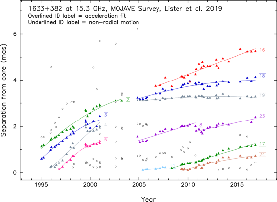
Figure 1.— Plot of angular separation from the core versus time for Gaussian jet features. The B1950 source name is given at the top left of each panel. Colored symbols indicate robust features for which kinematic fits were obtained. The identification number is overlined if the acceleration model was fit and indicated a $>3\sigma$ acceleration. An underlined identification number indicates a feature with non-radial motion. The $1\sigma$ positional errors on the individual points typically range from 10% of the FWHM restoring beam dimension for isolated compact features, to 20% of the FWHM for weak features. This corresponds to roughly 0.03 mas to 0.15 mas, depending on the source declination. (This is a figure stub; an extended version is available online.)

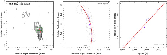
Figure 2.— Motion fits and sky position plots of individual robust jet features. Positions are relative to the core position. The left-hand panel shows a 15 GHz VLBA total intensity contour image of the jet at the epoch closest to the middle reference epoch. The green box delimits the zoomed region that is displayed in the middle panel. The feature’s position at the image epoch is indicated by the green cross-hairs. The dotted line connects the feature with the core feature and is plotted with the mean position angle. The position at the image epoch is shown by a filled blue circle while other epochs are plotted with unfilled blue circles. The red solid line indicates the vector fit (or accelerating fit, if there is significant acceleration) to the feature positions. The gray dashed circles / ellipses indicate the fitted FWHM sizes of the feature at the measured epochs. (This is a figure stub; an extended version is available online.)

3.2.1 Pattern Speeds

In a previous kinematic study (Lister et al., 2013), we found that in many individual AGN jets, there is no single apparent speed $\beta_{\mathrm{app}}=v_{\mathrm{app}}/c$ at which bright features propagate downstream. Instead, there is typically a single characteristic speed with a modest spread around this value. Since trackable features emerge only every few years in most bright blazar jets, continuous monitoring periods of a decade or more are needed to establish the characteristic speed of a jet, and whether any individual feature may have an atypically low pattern speed (see also a recent analysis of MOJAVE kinematics results by Plavin et al. 2018).

In Figure 3 we show the distribution of speed differences from the jet’s median speed for 436 features in 26 jets that have ten or more robust features. This plot contains nearly twice as many jet features as our previous kinematic study, and is qualitatively similar. Most features lie within $\pm 40$% of the jet’s median speed. There is also a small tail consisting of atypically fast features. The jet with the largest range of speeds is 4C $+$15.05 (0202$+$149), which has ten features with apparent speeds ranging from 0.1 $c$ to 16 $c$.

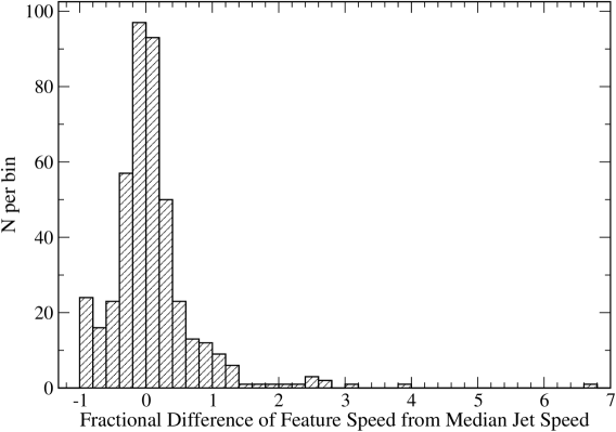
Figure 3.— Overall normalized speed distribution within jets with at least ten robust features. The fractional difference is defined as $(\mu-\mu_{\mathrm{median}})/\mu_{\mathrm{median}}$.

We have identified 55 features in 42 AGN jets that have appreciably slower speeds than other features in the same jet. Our specific criteria are that the feature (i) does not have a $>3\sigma$ acceleration, (ii) has an angular speed smaller than 20 $\;\mu{\rm as\ y}^{-1}\;$, and (iii) has a speed at least ten times slower than the fastest feature in the same jet. Figure 4 shows the distribution of projected distance from the core for 53 slow pattern speed features in 40 AGNs with known redshifts. The vast majority are located within 4 pc of the core feature ($\sim 100$ pc de-projected, given typical viewing angles $<2^{\circ}$). This is consistent with the 43 GHz VLBA survey of 36 AGNs by Jorstad et al. (2017), who found 21% of jet features to be quasi-stationary, with most located at projected core distances below 3 pc.

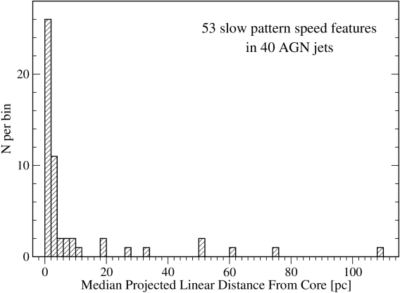
Figure 4.— Distribution of projected linear distance from the core feature in parsecs for 53 features classified as having a slow pattern speed.

Of the 1744 robust jet features that we have studied, only 44 (2.5%) have ‘velocity vectors that are directed inward toward the core feature. We might expect to see rare instances of apparent inward motion when a feature moving along a curved trajectory crosses our line of sight (e.g., as in the case of 4C +39.25; Alberdi et al. 2000). It is also possible that small changes in the brightness distribution of a large diffuse feature may alter its best-fit Gaussian centroid location, creating apparent inward motion. We note two instances (feature id = 1 in 87GB 061258.1+570222 and id = 1 in 8C 1944+838) where this may be the case. Inward motion can also result from incorrect identification of the core feature, or variable structure near the core that is below the angular resolution of our observations that may alter the fitted core location. We note that in 16 of 33 AGN jets with inward motion, the inward-moving feature is the closest feature to the core, and four of these jets (all associated with BL Lac objects: UGC 00773, 3C 66A, Mrk 421, ON 325) have more than one close-in inward-moving feature.

3.2.2 Speed Distributions

We have calculated maximum and median speed statistics for the jets in our sample using the method described in Lister et al. (2013). For accelerating features, we note that the speeds are determined at the middle epoch, and thus may not represent the maximum speed attained by the feature. In the case of two AGNs for which we could not identify any robust features (AO 0235+164 and 1ES 1959+650), we adopted maximum speeds from the literature based on VLBA observations made at other wavelengths. We plot the distributions of these statistics in Figure 5. Slow apparent speeds are common, with very few measured speeds above 30 $c$. As discussed by Vermeulen & Cohen (1994) and Lister & Marscher (1997), the shape of the distributions is incompatible with all jets having the same bulk Lorentz factor, and instead suggests a power law parent distribution that is weighted towards slow speeds. Single-valued parent $\Gamma$ distributions predict an excess of high apparent jet speeds, while Gaussian $\Gamma$ distributions do not reproduce the gradual fall-off in the number of jets with higher apparent speeds.

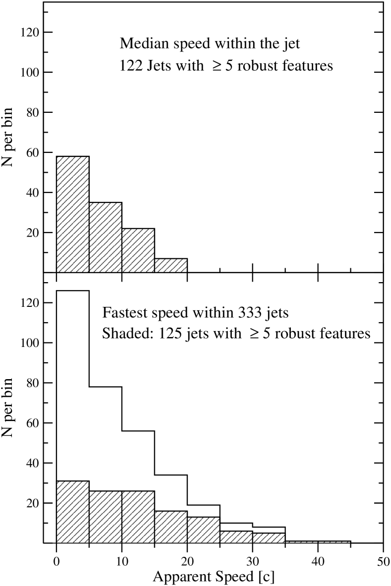
Figure 5.— Top panel: distribution of median apparent speed within 122 AGNs having at least five robust jet features. Bottom panel: distributions of maximum apparent speed for 333 AGN jets (unshaded) and 125 AGNs having at least five robust jet features (shaded).

3.2.3 Statistical Trends

In Figure 6 we plot maximum apparent jet speed versus rest frame synchrotron SED peak frequency. The plot includes AGNs from our survey, as well as those from Piner & Edwards (2018) and Jorstad et al. (2017). AGNs with $<3\sigma$ maximum speeds are indicated with upper limit symbols. The crosses indicate BL Lacs with no known redshift, and their extents correspond to lower and upper redshift limits published in the literature. For clarity, we have omitted BL Lacs for which the redshift limits give a possible range of $\beta_{\mathrm{app}}$ greater than 20. There is a clear upper envelope to the distribution, with the highest jet speeds being found only in AGNs with low synchrotron peak frequencies.

The filled symbols indicate AGNs that have been detected at TeV gamma-ray energies with the airshower telescopes VERITAS, HESS, or MAGIC. The large fraction of high synchrotron peaked (HSP) AGNs that are TeV-detected in this plot is a selection effect since these have been specifically targeted for long term VLBA kinematic study by Piner & Edwards (2018). The ISP AGNs have been targeted in MOJAVE on the basis of their detection at GeV energies by Fermi , while most of the low synchrotron peaked (LSP) AGNs are from the radio-selected MOJAVE sample (Lister et al., 2016). Although a fast jet speed does not guarantee a TeV detection, it does appear to be a minimum requirement for the intermediate- and low synchrotron peaked AGNs. This implies a direct connection between the bulk jet speed measured on parsec scales and the Doppler boosting level of the TeV emission. Of the 14 non-HSP TeV detected AGNs in Figure 6, only three have maximum jet speeds below 6 c. Two of these (3C 84 and M 87) are very nearby ($<75$ Mpc) radio galaxies, and the third (TXS 0506+056) is an unusual ISP BL Lac with a measured maximum speed of $0.98c\pm 0.3c$ that lies within the sky error circle of a high-energy neutrino event detected in 2017 (IceCube Collaboration et al., 2018).

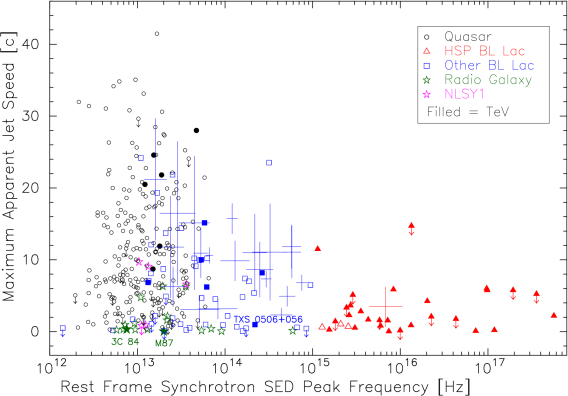
Figure 6.— Maximum apparent jet speed versus synchrotron peak frequency for jets in the MOJAVE survey, as well as those in the survey of Piner & Edwards (2018). Upper limit values are denoted by downward arrows. Quasars are indicated by black circles, radio galaxies by green stars, narrow-line Seyfert 1 galaxies by violet stars, high synchrotron peaked BL Lac objects by red triangles, and other BL Lac objects by blue squares. Filled symbols indicate detections by ground-based TeV gamma-ray observatories. The cross symbols indicate BL Lacs for which only upper and lower limits on the redshift are known.

4. MONTE CARLO JET PARENT POPULATION MODELING

The interpretation of parsec scale AGN jet kinematic studies presents a challenge in the sense that the individual objects that are most easily studied (i.e., high flux density, with proper motions observable on time periods of $\sim$ a few years) are blazars, whose selection is highly affected by Doppler bias (Scheuer & Readhead, 1979). In principle, the observed redshift, luminosity, and apparent speed distributions of a complete flux density-limited jet sample can be used to recover the intrinsic properties of the blazar parent population, but the Doppler selection effects need to be carefully accounted for. Vermeulen & Cohen (1994) and Lister & Marscher (1997) have shown that this can be done analytically only in the case of very simplistic, non-realistic assumptions. These include a non-evolving single power-law luminosity function and a single-valued or uniform distribution of bulk Lorentz factors, neither of which provide satisfactory fits to the data. The typical approach (e.g., Lister & Marscher 1997; Lister et al. 2009b; Bloom 2008; Giommi et al. 2012; Liodakis & Pavlidou 2015) has been to generate simulated flux density-limited samples from jet parent populations whose properties are drawn from specified probability distributions, and find the set of distribution parameters that best fit the data. In this section we carry out this type of Monte Carlo analysis on our MOJAVE data, based on the method of Lister & Marscher (1997).

4.1. Simulated Jet Properties

The observed flux density $S_{\nu}$ from a spherical optically thick source of radiation with an isotropically emitted rest frame luminosity $L_{\nu}\propto\nu^{\alpha}$, moving with bulk Lorentz factor $\Gamma$ at an angle $\theta$ to the line of sight and located at redshift $z$ (with corresponding luminosity distance $D_{L}(z)$) is (e.g., Blandford & Königl 1979; Condon & Matthews 2018)

$$S_{\nu}={L_{\nu}\delta^{p}\;(1+z)^{(1+\alpha)}\over 4\pi D_{L}^{2}(z)},$$ (3)

where $\nu$ is the observing frequency and $L_{\nu}$ is the luminosity emitted in the jet frame at that same frequency. The exponent $p$ of the Doppler factor

$$\delta=\left[\Gamma-\sqrt{(\Gamma^{2}-1)}\cos{\theta}\right]^{-1}$$ (4)

is $p=3-\alpha$ in the scenario described above. However, in the case of a continuous jet made up of many such spheres, one cannot distinguish the lifetimes of the individual emitting particles, and a time dilation factor of $\delta$ is no longer applicable, hence $p=2-\alpha$ (Cawthorne, 1991).

The minimum properties required to simulate the observed flux density of an AGN jet are therefore $z$, $L_{\nu}$, $\Gamma$, $\theta$, $\alpha$, and $p$. Actual AGN jets present complications in terms of the geometry of their emitting regions, optical depth variations, and flow accelerations, but the highest contributions to the observed flux density will come from regions where the synchrotron emission coefficient is highest, and where the Doppler factor is largest (e.g., $\theta\lesssim\cos^{-1}{\beta}$, where $\beta$ is the flow velocity in units of the speed of light). Stacked-epoch MOJAVE VLBA images of blazars show mainly conical jet profiles (Pushkarev et al., 2017) in which adiabatic expansion and synchrotron losses exponentially reduce the electron energies and magnetic field strength with distance down the jet (e.g., Konigl 1981). The bulk of the synchrotron emission therefore originates near the base of the jet, as confirmed by VLBI morphologies that typically consist of a bright optically thick core feature accompanied by a much weaker jet. The exceptions to this are (i) young AGN jets of the CSO/GPS class, which have high luminosity radio lobes that are interacting with the interstellar medium of the host galaxy (O’Dea, 1998), and (ii) rare instances where a bent downstream jet flow crosses the line of sight and experiences maximum Doppler boosting (e.g., 4C +39.35, Alberdi et al. 2000).

There are therefore good reasons to expect that a simulated population where each jet consists of a single (core) emitting region can provide a good representation of a suitably chosen blazar sample. The 1.5JyQC sample is well-suited in several respects, as it is a complete flux density-limited sample selected at high radio frequency, where the relative flux density contribution of the steep-spectrum downstream jet emission is low compared to the (typically flat-spectrum) core. It is also selected on the basis of VLBI flux density, which includes no contribution from any large kiloparsec scale emission. Any contaminating CSO/GPS sources can be rejected on the basis of available spectral and morphological information, and most importantly, the sample is large enough to statistically constrain the best fit parameters of the Monte Carlo simulations. After dropping two GPS quasars (PKS B0742+103 and OI $-$072) and six AGNs with no optical spectral information there are 174 1.5JyQC quasars with redshift $z\geq 0.15$ suitable for comparison with our simulations.

4.2. Simulation Parameters

Our simulation method is to generate a parent population of jets drawn from specified redshift, Lorentz factor, radio luminosity, and viewing angle distributions, calculate their predicted flux densities, and retain those jets that exceed the specified 1.5 Jy flux density limit. Because the 1.5JyQC sample includes all AGNs above declination $-30^{\circ}$ known to have exceeded 1.5 Jy over a 25 year period, we do not include any flux variability in our simulations, but instead compare our simulated jet flux densities to the maximum jet flux density for each AGN measured during the 1.5JyQC selection period (column 5 of Table 2).

4.2.1 Luminosity Function

Despite many studies on the radio luminosity functions (LFs) of AGNs, there is still no consensus on whether radio-loud AGN LFs evolve with lookback time in a manner consistent with increasing number density, increasing luminosity, or a mixture of both (Best et al., 2014; Smolčić et al., 2017; Yuan et al., 2018). There are also indications that lower power (i.e., FR I) AGNs may evolve differently than the high power (FR II) population (Rigby et al., 2008). Given these uncertainties, we have adopted a simple pure luminosity evolution parameterization for flat spectrum radio quasars used by Ajello et al. (2012) and Mao et al. (2017):

$$\Phi(L,z)\propto\Phi(L/e(z)),$$ (5)

where

$$e(z)=(1+z)^{k}e^{z/\eta},$$ (6)

and

$$\Phi(L/e(z=0))\propto L^{\gamma}.$$ (7)

Our approach is to find the best fit values of $\gamma$, $\eta$ and $k$ using the MOJAVE data. We restrict our comparisons to quasars in the 1.5JyQC sample only, given the possibility that the BL Lac objects may be drawn from a different (i.e., lower power, or FR I) parent population (Urry & Padovani, 1995). We set the lower limit on the parent LF at $10^{24}$ W Hz^-1 based on the least powerful known FR II radio galaxies (e.g., Antognini et al. 2012).

4.2.2 Redshift Distribution

By adopting a pure luminosity evolution model, we assume that the parent jet population has a constant co-moving density with redshift. All of the 1.5JyQC quasars have redshifts greater than 0.15, with the exception of TXS 0241+622 ($z=0.045$). In order to avoid small number statistics in this nearby volume of space, we drop this AGN from our data comparisons and set the lower redshift limit of our simulation to $z=0.15$. Because the form of LF evolution is not well known at very high redshift, we set the upper redshift limit in our simulations to that of the highest redshift 1.5JyQC quasar: OH 471 ($z=3.4$).

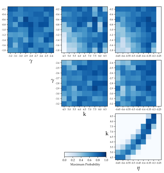
Figure 7.— Corner plot showing two-dimensional parameter space projections of the Lorentz factor distribution power law index $b$ and luminosity function evolution parameters $k$ and $\eta$ for the Monte Carlo parent population simulation grid with Doppler boosting index $p=2$. The false color scale corresponds to the maximum A-D test probability that the redshifts of the 1.5JyQC quasar sample and a simulation having that particular parameter combination are drawn from the same parent population. Lighter colors indicate poorer fits to the data.

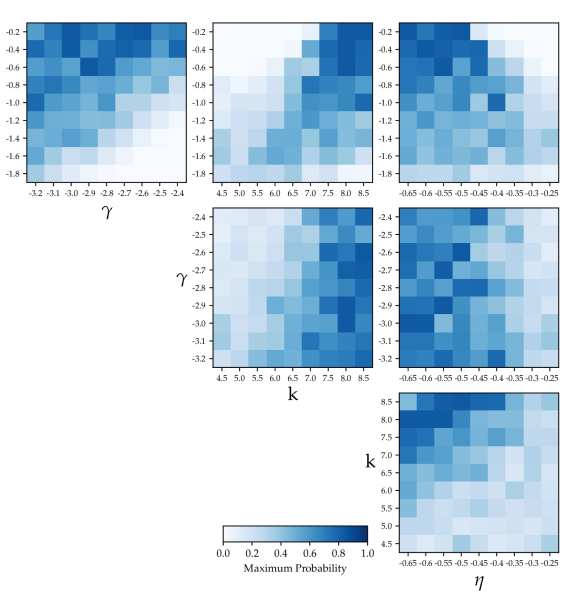
Figure 8.— Corner plot showing two-dimensional parameter space projections of the Lorentz factor distribution power law index $b$ and luminosity function evolution parameters $k$ and $\eta$ for the Monte Carlo parent population simulation grid with Doppler boosting index $p=2$. The false color scale corresponds to the maximum A-D test probability that the apparent jet speeds of the 1.5JyQC quasar sample and a simulation having that particular parameter combination are drawn from the same parent population. Lighter colors indicate poorer fits to the data.

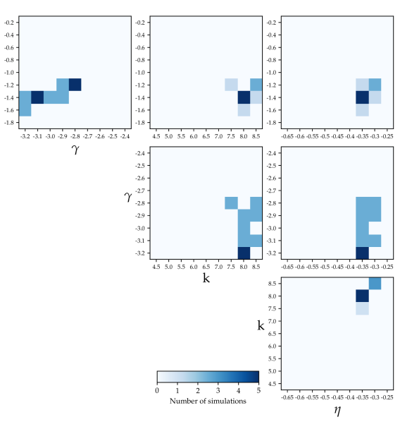
Figure 9.— Corner plot showing two-dimensional parameter space projections of the Lorentz factor distribution power law index $b$ and luminosity function evolution parameters $k$ and $\eta$ for the Monte Carlo parent population simulation grid with Doppler boosting index $p=2$. The false color scale corresponds to the number of simulations having that particular parameter combination that provide acceptable fits to the 1.5JyQC sample data.

4.2.3 Bulk Lorentz Factor Distribution and Doppler Boosting Index

Due to the strong selection biases associated with Doppler boosting, any large flux density-limited jet sample should contain some jets with the maximum Lorentz factor in the population (viewed at small $\theta$). In the MOJAVE sample the fastest instantaneous measured jet speed is approximately 50 $c$ for an accelerating feature in the jet of PKS 0805$-$07 (Lister et al., 2016), which corresponds to a $\Gamma_{\mathrm{max}}\simeq 50$ . In light of our discussion of the observed apparent velocity distributions in § 3.2.2, we adopt a power law Lorentz factor distribution for our simulated jets of the form $N(\Gamma)\propto\Gamma^{b}$, where $b$ is a free parameter with values less than zero and $\Gamma$ ranges from 1.25 to 50. The lower limit on $\Gamma$ ($\beta\simeq 0.6c$) is based on a Bayesian analysis of the relative prominence of radio cores and kiloparsec scale jets in FR II radio sources by Mullin & Hardcastle (2009). We assume no evolution of the jet Lorentz factor distribution with redshift.

The brightest radio-loud AGN cores are known to have a range of spectral indices with a mean value $\alpha=0.22\pm 0.03$ (Hovatta et al., 2014), however, the intrinsic distribution is not well known due to the difficulty of deconvolving relativistic beaming and projection effects. The spectral index enters into the simulated jet flux density via the small $(1+z)^{1+\alpha}$ k-correction, and more importantly, the Doppler boost index $p$. Any spread of $\alpha$ in the parent population will be effectively smoothed out in the observed luminosity function, so we fix $\alpha=0$ for all our simulated jets and assume continuous jet emission such that $p=2$. We discuss other fixed values of $\alpha$ in § 4.4.

The Monte Carlo analysis of Lister & Marscher (1997) included the possibility of an intrinsic correlation between jet Lorentz factor and synchrotron luminosity of the form $L\propto\Gamma^{\xi}$. They found that both $\xi=0$ and $\xi\neq 0$ models produced very similar fits to the Caltech-Jodrell Flat-Spectrum AGN sample data. As we will show in Section 4.4, we are able to obtain good fits to the 1.5JyQC quasar sample assuming no $L-\Gamma$ correlation, so we explore only the $\xi=0$ case in this paper.

4.3. Simulation Procedure

In order to search for the best fit parent population parameters, we constructed a grid of simulations with equally spaced parameter values spanning the ranges listed in Table 6. The procedure used to create each simulation in the grid is as follows:

(i) Select values for $b$, $\gamma$, $k$, and $\eta$.

(ii) Generate $z$, $L_{\nu}$, $\Gamma$, and $\theta$ values for a single jet from the probability distributions listed in Table 6.

(iii) Calculate the observed flux density of the jet according to Equation 3. We ignore any contribution from the counter-jet since it will be negligible for AGNs in a highly Doppler-biased sample (see § 4.4.1).

(iv) If $S_{\nu}>1.5$ Jy, keep the simulated jet.

(v) Repeat steps (ii) through (iv) until a sample of jets 10 times larger than the 1.5JyQC comparison sample is obtained, and record the total size of the parent population needed to produce this sample.

Table 6 Monte Carlo Jet Model Parameters

Jet Property	Distribution	Fixed parameters	Free parameter ranges
Lorentz factor	$N(\Gamma)d\Gamma\propto\Gamma^{b}$	$\Gamma_{\mathrm{min}}=1.25$	$-1.8\leq b\leq-0.2$, step = 0.2
		$\Gamma_{\mathrm{max}}=50$
Luminosity function	$\Phi(L,z)\propto\Phi(L/e(z))$	$L_{\mathrm{min}}=10^{24}$ W Hz-1	$-0.65\leq\eta\leq-0.25$, step = 0.05
	$e(z)=(1+z)^{k}e^{z/\eta}$	$L_{\mathrm{max}}=10^{31}$ W Hz-1	$4.5\leq k\leq 8.5$, step = 0.5
	$\Phi(L/e(z=0))\propto L^{\gamma}$		$-3.2\leq\gamma\leq-2.4$, step = 0.1
Beamed luminosity	$P=L\,\delta^{p}$	$p=2+\alpha$	$\alpha=-0.5$, 0, 0.22
Viewing angle	$p(\theta)d\theta=\sin{\theta}$	$\theta_{\mathrm{min}}=0^{\circ}$	$\cdots$
		$\theta_{\mathrm{max}}=90^{\circ}$

By creating larger samples than the data sample in step (v) we reduce the amount of statistical fluctuations associated with selecting a relatively small number of bright AGNs from a very large parent population. In doing so, we are effectively creating simulated jet samples from ten Universes and are comparing the mean properties of these samples to the data.

4.4. Comparisons to MOJAVE Data

For each simulation in the four dimensional parameter grid ($b$, $\gamma$, $k$, $\eta$) we compared the simulated flux density, redshift, radio luminosity ($P_{\nu}$), and apparent velocity distributions to the 1.5JyQC sample of 174 quasars using the Anderson-Darling (A-D) test. The latter is a non-parametric test that assesses whether two samples are drawn from different parent populations, and is sensitive to a wider variety of possible distribution differences than the frequently used Kolmogorov-Smirnov test (Engmann & Cousineau, 2011). Our method was to randomly select a sample of 174 jets from the simulation and perform the A-D tests against the 1.5JyQC sample. We repeated this process 10 times and recorded the median A-D test probabilities $p_{S}$, $p_{z}$, $p_{P}$, and $p_{\beta\mathrm{app}}$ , corresponding to the probability of the null hypothesis that the simulated and 1.5JyQC distributions are drawn from the same parent population. Since the completeness of the observational data is high (100% for $S$, $z$ and $P$, and 87% for $\beta_{\mathrm{app}}$), we did not use any bootstrapping procedures to simulate the missing data.

In Figure 7 we plot two-dimensional projections of the grid parameter space, where the false-color corresponds to the maximum value of $p_{z}$ for any simulation having that particular parameter combination. The 1.5JyQC redshift distribution serves to constrain the parameter space to a limited number of $k-\eta$ (evolution parameter) combinations, as seen in the lower right panel. The top row of plots in Fig. 7 indicates, however, that the 1.5JyQC redshifts can be well-reproduced with many different combinations of the parent LF and the Lorentz factor distribution parameters.

The two-dimensional projections in Figure 8, in which the false-color corresponds to the maximum values of $p_{\beta\mathrm{app}}$, serve to further constrain the region of viable parameter space for the simulations. The $\beta_{\mathrm{app}}$ distribution is best fit with simulations with $k>5.5$. Also, the values of $k$ and $\eta$ that provide the best fits to the 1.5JyQC apparent velocity distribution (lower right panel) yield relatively poor fits to the observed luminosity distribution.

Within the full grid, the simulation with the highest A-D probability summed over all four observable quantities has $b=-1.4$, $\gamma=-3.1$, $k=8.0$, $\eta=-0.35$ (model A). There are no other simulations in the grid that have an A-D probability greater than 0.4 in all four quantities. We investigated the effect of random statistical outliers on the A-D probability values for this best fit simulation by first creating a simulated flux density-limited sample of 174000 jets (i.e., 1000 Universes), then selecting a random subset of 174 jets to compare with the 1.5JyQC data. After repeating the random subset selection 1000 times, the standard deviations on $p_{S}$, $p_{z}$, $p_{P}$, and $p_{\beta\mathrm{app}}$ were 0.25, 0.3, 0.25, and 0.2 respectively. We therefore consider any simulation that has all four A-D probabilities within 1 $\sigma$ of those of the best fit simulation to also be an acceptable fit to the data.

In Figure 9 we show a corner plot with false color indicating the number of acceptable best fit simulations having particular parameter combinations. Based on the plot, we find acceptable fits for the parameter ranges $-1.6\leq a\leq-1.2$, $-3.2\leq\gamma\leq-2.8$, $7.5\leq k\leq 8$, and $-0.35\leq\eta\leq-0.30$.

We constructed two additional simulation grids to investigate whether better fits could be obtained using a fixed value of $\alpha=+0.22$ (corresponding to a Doppler boosting index of $p=1.78$), and $\alpha=-0.5$ (corresponding to $p=2.5$). The best fit simulation in the $p=1.78$ case (model B in Table 7) gave acceptable fits to the flux density, redshift, and luminosity distributions, but provided a relatively poor fit to the apparent speed distribution. Although the best fit simulation in the $p=2.5$ grid (model C) provided a good fit to the apparent speed distribution, none of the simulations in the grid gave A-D probabilities greater than 0.03 in all four observable parameters simultaneously.

Table 7 Best Fit Monte Carlo Grid Simulations

Model	Parameter						Anderson-Darling Test Probabilities
Name	$b$	$\gamma$	$k$	$\eta$	$\alpha$	$p$	$p_{S}$	$p_{z}$	$p_{P}$	$p_{\beta\mathrm{app}}$
A	$-$1.40	$-$3.1	8.0	$-$0.35	0	2	0.65	0.43	0.52	0.40
B	$-$1.00	$-$2.6	8.5	$-$0.30	0.22	1.78	0.70	0.67	0.24	0.10
C	$-$1.40	$-$3.2	7.0	$-$0.35	$-$0.5	2.5	0.13	0.044	0.026	0.46

Note. — The simulation parameters are defined in Table 6. Model A has the highest overall Anderson-Darling test probability sum $p_{S}$+ $p_{z}$+ $p_{P}$+ $p_{\beta\mathrm{app}}$ of any grid simulation.

4.4.1 Best Fit Parent Population Properties

In Figure 10 we show the distributions of observable quantities for the 1.5JyQC quasar sample (red lines), as well as our best fit (model A) simulation. The blue bands represent 1$\sigma$ ranges on the bin values that we derived by producing a simulation 1000 times the size of the 1.5JyQC, and then randomly choosing a sub-sample of 174 jets from it, repeating the latter step 10000 times. We note that the simulation plotted in Fig. 10 provides the best overall fit to the data, however, other combinations of fit parameters gave better fits to individual observable quantities. We have scaled the simulated apparent speed distribution in the top right panel by a factor of $151/174=0.87$ to take into account the 23 missing jet speeds in the 1.5JyQC quasar sample.

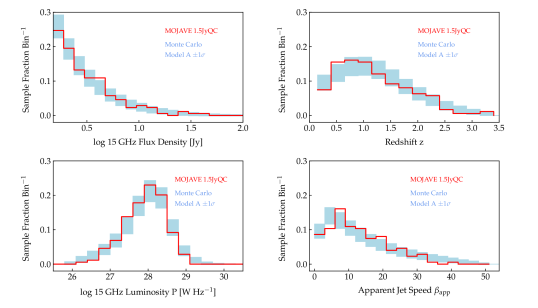
Figure 10.— Histograms of observable jet properties for the MOJAVE 1.5JyQC quasar sample (red lines). The blue bands indicate the $\pm 1\sigma$ ranges on the bin values obtained by drawing 10000 samples of 174 jets from the best fit Monte Carlo simulation.

We plot the distributions of several intrinsic (indirectly observable) quantities from our best fit simulation A in Figure 11. As expected from Doppler orientation bias, nearly all of the quasar jets in the 1.5JyQC sample are predicted to have viewing angles less than $\sim 10^{\circ}$ from the line of sight, with the distribution peaking at $2^{\circ}$. The bottom left panel shows the distribution in terms of the critical angle $\theta_{\mathrm{cr}}=\sin^{-1}{(1/\Gamma)}$, and indicates that the most likely viewing angle is not $\theta_{\mathrm{crit}}$ as commonly cited in the literature, but approximately half of this value (e.g., Vermeulen & Cohen 1994; Lister & Marscher 1997; Cohen et al. 2007). The top middle panel shows the Lorentz factor distribution, which is broadly peaked between $\Gamma\simeq 5$ and $\Gamma\simeq 15$, with a rapid falloff past $\Gamma=20$. The breadth of the $\Gamma$ distribution indicates that adopting a single value of $\Gamma=10$ for all blazars is not well supported by the observational data. The Doppler factor distribution has a similar shape to the $\Gamma$ distribution, and peaks at $\delta\simeq 10$, declining rapidly past $\delta\simeq 30$.

Liodakis et al. (2018) recently carried out a Bayesian light curve analysis of OVRO 15 GHz monitoring data on the original 1.5 Jy sample and calculated variability Doppler factors and distributions of Lorentz factor and viewing angle. We find a high degree of consistency between these distributions for the 1.5 Jy quasars and those of our best fit Monte Carlo simulation in Fig. 11.

In the bottom middle panel we plot the distribution of intrinsic (unbeamed) luminosity $L$. Although the intrinsic parent LF peaks at $L\simeq 10^{24}$ W Hz^-1, most of the jets in the simulated flux density-limited sample have intrinsic (unbeamed) luminosities roughly an order of magnitude higher due to the combined effects of Doppler and Malmquist bias. This implies that the parent population of the brightest radio quasars consists of powerful FR II radio galaxies with a relatively narrow range of unbeamed 15 GHz radio luminosity between $\sim 10^{25}$ and $\sim 10^{26}$ W Hz^-1.

Liodakis et al. (2017) used Monte Carlo simulations to investigate the predicted distribution of jet-counterjet flux density ratios due to relativistic beaming in flux density-limited blazar samples. In the bottom right panel of Fig. 11 we plot the distribution of this quantity for our best fit model. We obtain very similar results, with most jets having ratios of $10^{4}$ to $10^{7}$. These are much higher than can be probed in our snapshot MOJAVE VLBA images, given their image rms levels of $\sim 0.1$ mJy beam^-1 and typical jet brightnesses of $<100$ mJy beam^-1 downstream from the core.

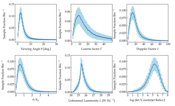
Figure 11.— Histograms of intrinsic jet properties for the best fit Monte Carlo simulation of the 1.5JyQC quasar sample. The blue bands indicate the $\pm 1\sigma$ ranges on the bin values obtained by drawing 1000 samples of 174 jets from the simulation.

In Figure 12 we plot the distribution of parent population sizes for the 10000 sub-samples, which is approximately Gaussian. For our best fit simulation parameters, typically $(3.5\pm 0.3)\times 10^{5}$ parent jets are needed to reproduce the 174 quasar jets in the MOJAVE 1.5JyQC sample. Given the co-moving simulated volume of 1334 Gpc³, this implies a parent space density of $261\pm 19$ Gpc^-3, which is comparable to the value of 200 Gpc^-3 obtained for FR II radio galaxies by Snellen & Best (2001) using the LF of Dunlop & Peacock (1990).

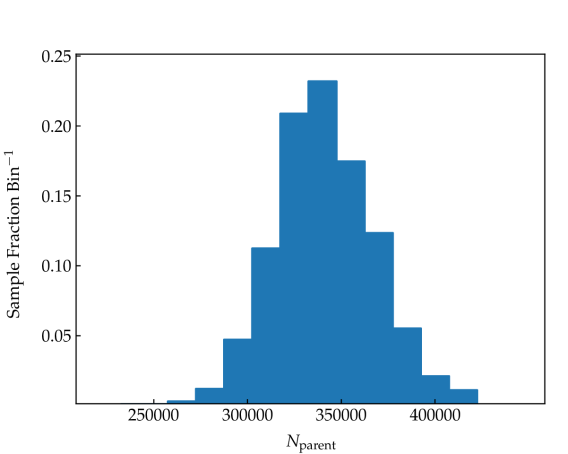
Figure 12.— Distribution of parent population size in the best fit Monte Carlo simulation that is required to produce each of 1000 sub-samples of 174 jets matching the MOJAVE 1.5JyQC properties.

A rule of thumb sometimes used in the literature is that for every blazar jet found in a survey with Lorentz factor $\Gamma$ there are $\Gamma^{2}$ parent jets (e.g., Mutel 1990; Ghisellini 2000; Berton et al. 2016). This assumption is based on the ratio of solid angle subtended by blazar jets viewed within the critical angle $1/\Gamma$ and the full range of jet viewing angle in the parent population, but fails to properly take into account the biases of flux density-limited sampling.

In Figure 13 we plot for our best fit Monte Carlo simulation the number of parent jets divided by the number of simulated $S_{\nu}>1.5$ Jy jets in binned intervals of Lorentz factor between 1 and 50. For $\Gamma\gtrsim 15$, there is a shallow increase in the predicted number of parent jets for each jet found with a particular Lorentz factor in the 1.5JyQC sample, from $N\sim 750$ to $N\sim 1300$ at $\Gamma=50$. This is much shallower than the rule of thumb $\Gamma^{2}$ dependence, and is a result of the fact that (i) very high $\Gamma$ jets are rare in the parent population, and (ii) most of these high $\Gamma$ jets do not exceed the 1.5 Jy flux density cutoff not only due to their viewing angle, but also their redshift and/or unbeamed luminosity. The large range of possible parent sizes for $\Gamma>40$ reflects the statistical fluctuations associated with selecting from this small cohort of jets in a flux density-limited sample.

A different behavior is seen below $\Gamma\simeq 15$. These jets are abundant in the parent population, yet most have low unbeamed luminosities and require either substantial Doppler boosting or a low redshift to exceed the flux density cutoff. Every low $\Gamma$ jet in the 1.5JyQC requires significantly more parent objects, since its maximum possible Doppler boost is only $(2\Gamma)^{p}$. This is the exact opposite of the $N\propto\Gamma^{2}$ prediction.

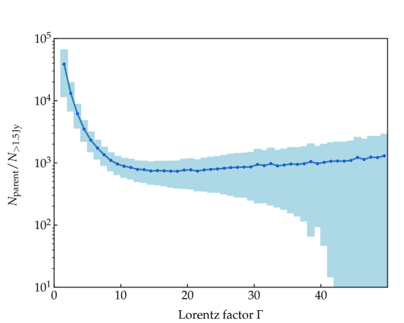
Figure 13.— Mean number of jets in the parent population divided by the mean number of jets exceeding 1.5 Jy in binned intervals of Lorentz factor for the best fit Monte Carlo simulation. The blue bands indicate the $\pm 1\sigma$ ranges on the bin values obtained by drawing 1000 samples of 174 jets from the simulation.

5. SUMMARY AND CONCLUSIONS

We have carried out a study of the parsec-scale jet kinematics of 409 bright radio-loud AGNs above declination $-30^{\circ}$, based on 15 GHz VLBA data obtained between 1994 August 31 and 2016 December 26. These AGNs have been part of the 2cm VLBA survey or MOJAVE programs, and have $\gtrsim 0.1$ Jy of correlated flux density at 15 GHz. By modeling the jet emission with a series of Gaussians in the interferometric visibility plane, we identified and tracked 1744 individual features in 382 jets over at least five epochs. We fitted their sky trajectories with simple radial and vector motion models, and additionally carried out a constant acceleration fit for 881 features that had ten or more epochs.

A primary goal of the MOJAVE program is to characterize the jet properties of a well-defined flux density-limited sample in order to better understand the blazar parent population. Using the extensive OVRO and UMRAO single-dish monitoring databases, as well as the MOJAVE VLBA archive, we constructed the MOJAVE 1.5 Jy Quarter Century sample, which consists of all 232 AGNs north of J2000 declination $-30^{\circ}$ that are known to have exceeded 1.5 Jy in 15 GHz VLBA correlated flux density between 1994.0 and 2019.0. We carried out Monte Carlo simulations to determine the best fit parent population parameters that reproduced the redshift, radio luminosity, and apparent velocity distributions of the 174 quasars with $z\geq 0.15$ in the 1.5JyQC sample.

We summarize our conclusions as follows:

1. A total of 382 of 409 jets had at least one robust bright feature that could be tracked for five or more epochs. A majority (59%) of the well-sampled jet features showed evidence of accelerated motion at the $>3\sigma$ level.

2. We examined the distribution of apparent speeds within 26 individual jets that had ten or more robust features, and confirmed that each jet tends to have a characteristic speed that is likely related to the underlying flow. Other than a few fast outliers and some slow pattern speeds, the speeds of features in a jet typically lie within $\sim\pm 40\%$ of the characteristic speed.

3. We were able to identify 55 features in 42 jets that had unusually slow pattern speeds ($\mu<20$ $\;\mu{\rm as\ y}^{-1}\;$and at least 10 times slower than the fastest feature in the jet). We confirm the 43 GHz VLBA results of Jorstad et al. (2017) that the vast majority of these lie within 4 pc (projected) of the core feature, and may represent quasi-stationary standing shocks near the jet base.

4. Only 2.5% of the features we studied had velocity vectors directed inward toward the core. In some cases, these are likely due to brightness variations affecting the fitted centroid position of a large diffuse feature, or a feature on a bent trajectory that is crossing the line of sight. In other cases there may be a mis-identification of the true core position. We find that in 16 of the 32 jets with apparent inward motion, the inward-moving feature is the closest feature to the core, and that four BL Lac jets have more than one close-in inward-moving feature.

5. We examined the distribution of maximum apparent jet speed for the AGNs in our full sample and the 1.5JyQC sample, and find that it is peaked at low values, with very few speeds above 30 $c$. Given the fact that large Doppler-biased jet samples should contain examples of the fastest jets in the parent population, and that our survey has not measured any instantaneous speeds above 50 $c$, this implies that the parent distribution of jet Lorentz factors is not single-valued, but is weighted towards low $\Gamma$, with decreasing numbers of jets up to $\Gamma_{\mathrm{max}}=50$.

6. We find a strong correlation between apparent jet speed and synchrotron peak frequency, with the highest jet speeds being found only in AGNs with low $\nu_{p}$ values. Although a fast jet speed does not guarantee that a jet will be detected at TeV gamma-ray energies, it appears to be a minimum requirement for LSP and ISP AGNs. The exceptions to date are the two very nearby radio galaxies 3C 84 and M87, and the BL Lac TXS 0506+056 that has been associated with a high energy neutrino detection event.

7. Our large grid of Monte Carlo parent population simulations yielded several parameter combinations that could adequately reproduce the flux density, redshift, radio luminosity, and apparent velocity distributions of the 174 quasars in the 1.5JyQC sample. These simulations have an unbeamed luminosity function above $10^{24}$ Hz with power law slope $-3.2\leq\gamma\leq-2.8$, and pure luminosity evolution of the form $e(z)=(1+z)^{k}e^{z/\eta}$, where $7.5\leq k\leq 8$ and $-0.35\leq\eta\leq-0.30$. The parent jet population has a power law distribution of Lorentz factors with slope $-1.6\leq b\leq-1.2$, ranging from $\Gamma=1.25$ to $\Gamma=50$, and a Doppler boosting index $p=2$. The best fit parent population (with $b=-1.4$, $\gamma=-3.1$, $k=8.0$, and $\eta=-0.35$) has a space density of $261\pm 19$ Gpc^-3, which is consistent with that of FR II radio galaxies. Most of the quasars in the 1.5JyQC have a relatively narrow range of intrinsic (unbeamed) parsec-scale 15 GHz radio luminosity between $\sim 10^{24.5}$ W Hz^-1 and $\sim 10^{26.5}$ W Hz^-1.

8. Our best fit simulation indicates that nearly all of the 1.5JyQC quasar jets are viewed at less than $\sim 10^{\circ}$ from the line of sight, with the distribution peaking at $2^{\circ}$. As previously discussed by Vermeulen & Cohen (1994); Lister & Marscher (1997) and Cohen et al. (2007), the most probable jet viewing angle is $\sim$ 0.5 times the critical angle $\theta_{\mathrm{cr}}=\sin^{-1}(1/\Gamma)$ where $\beta_{\mathrm{app}}=\Gamma\beta$.

9. The Lorentz factor distribution of the 174 bright radio quasars in the flux density-limited 1.5JyQC sample peaks between $\Gamma=5$ and $\Gamma=15$, with a rapid falloff past $\Gamma=20$. The breadth of the $\Gamma$ distribution indicates that adopting a single value of $\Gamma=10$ for all blazars is not well supported by the observational data. The Doppler factor distribution has a similar shape to the $\Gamma$ distribution, and peaks at $\delta\simeq 10$, declining rapidly past $\delta\simeq 30$. Both distributions are similar to those inferred from variability Doppler factor estimates using OVRO 15 GHz monitoring data by Liodakis et al. (2018).

10. We find that the oft-cited rule of thumb that for every jet found in a survey with Lorentz factor $\Gamma$ there are $\Gamma^{2}$ parent jets is incorrect for flux density-limited blazar samples. Above $\Gamma\simeq 15$, there is only a shallow increase in the expected number of parent jets per source with $\Gamma$, while for lower Lorentz factors, the number of parent jets increases rapidly with decreasing $\Gamma$.

References

- Abdo et al. (2009a) Abdo, A. A., et al. 2009a, ApJ, 707, 55
- Abdo et al. (2009b) —. 2009b, ApJ, 707, L142
- Ackermann et al. (2011) Ackermann, M., et al. 2011, ApJ, 743, 171
- Ackermann et al. (2015) —. 2015, ApJ, 810, 14
- Ajello et al. (2012) Ajello, M., et al. 2012, ApJ, 751, 108
- Ajello et al. (2017) —. 2017, ApJS, 232, 18
- Alberdi et al. (2000) Alberdi, A., Gómez, J. L., Marcaide, J. M., Marscher, A. P., & Pérez-Torres, M. A. 2000, A&A, 361, 529
- Aller et al. (1985) Aller, H. D., Aller, M. F., Latimer, G. E., & Hodge, P. E. 1985, ApJS, 59, 513
- Antognini et al. (2012) Antognini, J., Bird, J., & Martini, P. 2012, ApJ, 756, 116
- Berton et al. (2016) Berton, M., et al. 2016, A&A, 591, A98
- Best et al. (2014) Best, P. N., Ker, L. M., Simpson, C., Rigby, E. E., & Sabater, J. 2014, MNRAS, 445, 955
- Blandford et al. (2018) Blandford, R., Meier, D., & Readhead, A. 2018, arXiv e-prints, 1812.06025
- Blandford & Königl (1979) Blandford, R. D., & Königl, A. 1979, ApJ, 232, 34
- Bloom (2008) Bloom, S. D. 2008, AJ, 136, 1533
- Cawthorne (1991) Cawthorne, T. V. 1991, in Beams and Jets in Astrophysics, ed. Hughes, P. A. (Cambridge Astrophysics Series), 187–231
- Chang et al. (2017) Chang, Y.-L., Arsioli, B., Giommi, P., & Padovani, P. 2017, A&A, 598, A17
- Cohen et al. (2007) Cohen, M. H., Lister, M. L., Homan, D. C., Kadler, M., Kellermann, K. I., Kovalev, Y. Y., & Vermeulen, R. C. 2007, ApJ, 658, 232
- Condon & Matthews (2018) Condon, J. J., & Matthews, A. M. 2018, PASP, 130, 073001
- Deller et al. (2011) Deller, A. T., et al. 2011, PASP, 123, 275
- Dunlop & Peacock (1990) Dunlop, J. S., & Peacock, J. A. 1990, MNRAS, 247, 19
- Engmann & Cousineau (2011) Engmann, S., & Cousineau, D. 2011, Journal of Applied Quantitative Methods, 6, 1
- Fomalont (1999) Fomalont, E. B. 1999, in Astronomical Society of the Pacific Conference Series, Vol. 180, Synthesis Imaging in Radio Astronomy II, ed. G. B. Taylor, C. L. Carilli, & R. A. Perley, 301
- Ghisellini (2000) Ghisellini, G. 2000, in Recent Developments in General Relativity, ed. B. Casciaro, D. Fortunato, M. Francaviglia, & A. Masiello (Springer), 5–7
- Giommi et al. (2012) Giommi, P., Padovani, P., Polenta, G., Turriziani, S., D’Elia, V., & Piranomonte, S. 2012, MNRAS, 420, 2899
- Hervet et al. (2015) Hervet, O., Boisson, C., & Sol, H. 2015, A&A, 578, A69
- Homan et al. (2009) Homan, D. C., Kadler, M., Kellermann, K. I., Kovalev, Y. Y., Lister, M. L., Ros, E., Savolainen, T., & Zensus, J. A. 2009, ApJ, 706, 1253
- Homan et al. (2015) Homan, D. C., Lister, M. L., Kovalev, Y. Y., Pushkarev, A. B., Savolainen, T., Kellermann, K. I., Richards, J. L., & Ros, E. 2015, ApJ, 798, 134
- Homan et al. (2002) Homan, D. C., Ojha, R., Wardle, J. F. C., Roberts, D. H., Aller, M. F., Aller, H. D., & Hughes, P. A. 2002, ApJ, 568, 99
- Hook et al. (1996) Hook, I. M., McMahon, R. G., Irwin, M. J., & Hazard, C. 1996, MNRAS, 282, 1274
- Hovatta et al. (2014) Hovatta, T., et al. 2014, AJ, 147, 143
- IceCube Collaboration et al. (2018) IceCube Collaboration et al. 2018, Science, 361, 147
- Jones et al. (2005) Jones, D. H., Saunders, W., Read, M., & Colless, M. 2005, PASA, 22, 277
- Jorstad et al. (2017) Jorstad, S. G., et al. 2017, ApJ, 846, 98
- Kellermann et al. (1998) Kellermann, K. I., Vermeulen, R. C., Zensus, J. A., & Cohen, M. H. 1998, AJ, 115, 1295
- Komatsu et al. (2009) Komatsu, E., et al. 2009, ApJS, 180, 330
- Konigl (1981) Konigl, A. 1981, ApJ, 243, 700
- Kovalev et al. (2002) Kovalev, Y. Y., Kovalev, Y. A., Nizhelsky, N. A., & Bogdantsov, A. B. 2002, PASA, 19, 83
- LAMOST DR4 (2018) LAMOST DR4. 2018, http://dr4.lamost.org/
- Landoni et al. (2012) Landoni, M., Falomo, R., Treves, A., Sbarufatti, B., Decarli, R., Tavecchio, F., & Kotilainen, J. 2012, A&A, 543, A116
- Lawrence et al. (1986) Lawrence, C. R., Pearson, T. J., Readhead, A. C. S., & Unwin, S. C. 1986, AJ, 91, 494
- Liodakis et al. (2018) Liodakis, I., Hovatta, T., Huppenkothen, D., Kiehlmann, S., Max-Moerbeck, W., & Readhead, A. C. S. 2018, ApJ, 866, 137
- Liodakis & Pavlidou (2015) Liodakis, I., & Pavlidou, V. 2015, MNRAS, 451, 2434
- Liodakis et al. (2017) Liodakis, I., Pavlidou, V., & Angelakis, E. 2017, MNRAS, 465, 180
- Lister et al. (2018) Lister, M. L., Aller, M. F., Aller, H. D., Hodge, M. A., Homan, D. C., Kovalev, Y. Y., Pushkarev, A. B., & Savolainen, T. 2018, ApJS, 234, 12
- Lister & Homan (2005) Lister, M. L., & Homan, D. C. 2005, AJ, 130, 1389
- Lister & Marscher (1997) Lister, M. L., & Marscher, A. P. 1997, ApJ, 476, 572
- Lister et al. (2009a) Lister, M. L., et al. 2009a, AJ, 137, 3718
- Lister et al. (2009b) —. 2009b, AJ, 138, 1874
- Lister et al. (2011) —. 2011, ApJ, 742, 27
- Lister et al. (2013) —. 2013, AJ, 146, 120
- Lister et al. (2016) —. 2016, AJ, 152, 12
- Mao et al. (2017) Mao, P., Urry, C. M., Marchesini, E., Landoni, M., Massaro, F., & Ajello, M. 2017, ApJ, 842, 87
- Meyer et al. (2011) Meyer, E. T., Fossati, G., Georganopoulos, M., & Lister, M. L. 2011, ApJ, 740, 98
- Mullin & Hardcastle (2009) Mullin, L. M., & Hardcastle, M. J. 2009, MNRAS, 398, 1989
- Mutel (1990) Mutel, R. 1990, in Parsec-scale radio jets, ed. J. A. Zensus & T. J. Pearson (Cambridge University Press), 110–116
- Nieppola et al. (2006) Nieppola, E., Tornikoski, M., & Valtaoja, E. 2006, A&A, 445, 441
- Nieppola et al. (2008) Nieppola, E., Valtaoja, E., Tornikoski, M., Hovatta, T., & Kotiranta, M. 2008, A&A, 488, 867
- O’Dea (1998) O’Dea, C. P. 1998, PASP, 110, 493
- Paiano et al. (2017) Paiano, S., Landoni, M., Falomo, R., Treves, A., Scarpa, R., & Righi, C. 2017, ApJ, 837, 144
- Pâris et al. (2017) Pâris, I., et al. 2017, A&A, 597, A79
- Piner & Edwards (2018) Piner, B. G., & Edwards, P. G. 2018, ApJ, 853, 68
- Piner et al. (2010) Piner, B. G., Pant, N., & Edwards, P. G. 2010, ApJ, 723, 1150
- Plavin et al. (2018) Plavin, A. V., Kovalev, Y. Y., Pushkarev, A. B., & Lobanov, A. P. 2018, MNRAS, submitted; arXiv e-prints, 1811.02544
- Pushkarev et al. (2017) Pushkarev, A. B., Kovalev, Y. Y., Lister, M. L., & Savolainen, T. 2017, MNRAS, 468, 4992
- Richards et al. (2011) Richards, J. L., et al. 2011, ApJS, 194, 29
- Rigby et al. (2008) Rigby, E. E., Best, P. N., & Snellen, I. A. G. 2008, MNRAS, 385, 310
- Sargent (1970) Sargent, W. L. W. 1970, ApJ, 160, 405
- Scheuer & Readhead (1979) Scheuer, P. A. G., & Readhead, A. C. S. 1979, Nature, 277, 182
- Schneider et al. (1999) Schneider, D. P., Schmidt, M., & Gunn, J. E. 1999, AJ, 117, 40
- Schneider et al. (2010) Schneider, D. P., et al. 2010, AJ, 139, 2360
- Schramm et al. (1994) Schramm, K.-J., Borgeest, U., Kuehl, D., von Linde, J., Linnert, M. D., & Schramm, T. 1994, A&AS, 106, 349
- Shaw et al. (2013a) Shaw, M. S., Filippenko, A. V., Romani, R. W., Cenko, S. B., & Li, W. 2013a, AJ, 146, 127
- Shaw et al. (2012) Shaw, M. S., et al. 2012, ApJ, 748, 49
- Shaw et al. (2013b) —. 2013b, ApJ, 764, 135
- Shepherd (1997) Shepherd, M. C. 1997, in Astronomical Society of the Pacific Conference Series, Vol. 125, Astronomical Data Analysis Software and Systems VI, ed. G. Hunt & H. E. Payne (San Francisco: ASP), 77
- Smolčić et al. (2017) Smolčić, V., et al. 2017, A&A, 602, A6
- Snellen & Best (2001) Snellen, I. A. G., & Best, P. N. 2001, MNRAS, 328, 897
- Sowards-Emmerd et al. (2005) Sowards-Emmerd, D., Romani, R. W., Michelson, P. F., Healey, S. E., & Nolan, P. L. 2005, ApJ, 626, 95
- Stickel & Kuhr (1993) Stickel, M., & Kuhr, H. 1993, A&AS, 101, 521
- Stratta et al. (2011) Stratta, G., Capalbi, M., Giommi, P., Primavera, R., Cutini, S., Gasparrini, D., & on behalf of the ASDC team. 2011, ArXiv e-prints, 1103.0749
- Thompson et al. (1992) Thompson, D. J., Djorgovski, S., Vigotti, M., & Grueff, G. 1992, ApJS, 81, 1
- Urry & Padovani (1995) Urry, C. M., & Padovani, P. 1995, PASP, 107, 803
- Vermeulen & Cohen (1994) Vermeulen, R. C., & Cohen, M. H. 1994, ApJ, 430, 467
- Wright et al. (1983) Wright, A. E., Ables, J. G., & Allen, D. A. 1983, MNRAS, 205, 793
- Xiong et al. (2015) Xiong, D., Zhang, X., Bai, J., & Zhang, H. 2015, MNRAS, 450, 3568
- Yuan et al. (2018) Yuan, Z., Wang, J., Worrall, D. M., Zhang, B.-B., & Mao, J. 2018, ApJS, 239, 33
- Zensus et al. (2002) Zensus, J. A., Ros, E., Kellermann, K. I., Cohen, M. H., Vermeulen, R. C., & Kadler, M. 2002, AJ, 124, 662