Chandra-HETGS Characterization of an Outflowing Wind in the accreting millisecond pulsar IGR J17591$-$2342

Abstract

IGR J17591$-$2342 is an accreting millisecond X-ray pulsar discovered in 2018 August in scans of the Galactic bulge and center by the INTEGRAL X-ray and gamma-ray observatory. It exhibited an unusual outburst profile with multiple peaks in the X-ray, as observed by several X-ray satellites over three months. Here we present observations of this source performed in the X-ray/gamma-ray and near infrared domains, and focus on a simultaneous observation performed with the Chandra-High Energy Transmission Gratings Spectrometer (HETGS) and the Neutron Star Interior Composition Explorer (NICER). HETGS provides high resolution spectra of the Si-edge region, which yield clues as to the source’s distance and reveal evidence (at 99.999% significance) of an outflow with a velocity of $\mathrm{2\,800\,km\,s^{-1}}$. We demonstrate good agreement between the NICER and HETGS continua, provided that one properly accounts for the differing manners in which these instruments view the dust scattering halo in the source’s foreground. Unusually, we find a possible set of Ca lines in the HETGS spectra (with significances ranging from 97.0% to 99.7%). We hypothesize that IGR J17591$-$2342 is a neutron star low mass X-ray binary at a distance of the Galactic bulge or beyond that may have formed from the collapse of a white dwarf system in a rare, calcium rich Type Ib supernova explosion.

1 Introduction

Accreting msec X-ray pulsars (AMXPs) are a peculiar subclass of Neutron Star (NS) Low Mass X-ray Binaries (LMXBs). In general, no X-ray pulsations are detected in classical NS LMXBs: the magnetic field of the NS is believed to be too faint (${\mathrel{\hbox to0.0pt{\raise 2.20013pt\hbox{$<$}\hss}{\lower 2.20013pt\hbox{$\sim$}}}}10^{9}$ G) to channel the accreting matter — provided by the low mass companion star — and it ends up being buried in the accretion flow, producing a ‘spot-less’ accretion on the NS surface. In some cases, however, an X-ray pulsation is detected: it can be hundreds of seconds (e.g., $\sim$120 s, spinning down to $\sim$180 s over 40 years in the case of GX 1+4; see Jaisawal et al. 2018) down to the millisecond domain, in the range of 1.7–9.5 ms (e.g., Patruno & Watts, 2012; Campana & Di Salvo, 2018), the so-called accreting msec X-ray pulsars. Currently 21 such systems are known (Campana & Di Salvo, 2018). The fast pulsations are believed to be the result of long-lasting mass transfer from an evolved companion via Roche lobe overflow, resulting in a spin up of the NS (the recycling scenario; Alpar et al., 1982). These sources are very important because they provide the evolutionary link between accreting LMXBs and the rotation powered millisecond radio pulsars (MSP). Indeed, such a link has been recently observed in a few systems where a transition from the radio MSP phase (rotation powered) to the X-ray AMXP phase (accretion powered) has been detected (transitional MSP; Papitto, 2016, and references therein).

IGR J17591$-$2342 was discovered by INTEGRAL during monitoring observations of the Galactic Centre (PI J. Wilms) and bulge (PI E. Kuulkers). The source was detected in a 20–40 keV IBIS/ISGRI (15 keV – 1 MeV; Lebrun et al. 2003) mosaic image spanning 2018 August 10–11 (MJD 58340–58341) at a significance of approximately 9 $\sigma$ with a positional uncertainty of 3 arcmin (Ducci et al., 2018). IGR J17591$-$2342 was located at the rim of the field of view of the co-aligned, smaller field of view instrument JEM-X (3–35 keV, Lund et al. 2003), and hence was not detected in this lower energy bandpass field.

Subsequent observations with the Neil Gehrels Swift satellite refined the position to within a 3.6″ uncertainty (90% confidence level) and gave a preliminary estimate of the source’s absorbed 0.3–10 keV X-ray flux of $(2.6\pm 0.2)\times 10^{-10}\,\mathrm{erg\,cm^{-2}\,s^{-1}}$ (Bozzo et al., 2018). The spectrum was consistent with a highly absorbed powerlaw ($N_{\mathrm{H}}=(4.2\pm 0.8)\times 10^{22}\,\mathrm{cm^{-2}}$, $\Gamma=1.7\pm 0.3$). Optical follow up observations did not definitively reveal any counterpart within the Swift error circle (Russell & Lewis, 2018); however, radio observations showed a counterpart with a flux of $1.09\pm 0.02$ mJy at $\alpha_{\mathrm{J2000.0}}=17:59:02.86$, $\delta_{\mathrm{J2000.0}}=-23:43:08.0$ (0.6″ uncertainty), which is within 2.1″ of the Swift position (Russell et al., 2018a).

Joint Neutron Star Interior Composition Explorer (NICER)/NuSTAR observations demonstrated that this radio and X-ray source was in fact an accreting millisecond X-ray pulsar with a spin frequency of 527 Hz and an 8.8 hr orbital period with a likely companion mass $>0.42\,\mathrm{M_{\odot}}$ (Ferrigno et al., 2018; Sanna et al., 2018). The pulsar spin was detected in both instruments. The 3–30 keV NuSTAR absorbed flux was $4.2\times 10^{-10}\,\mathrm{erg\,cm^{-2}\,s^{-1}}$ and the extrapolated 0.1–10 keV NICER flux was $1.3\times 10^{-10}\,\mathrm{erg\,cm^{-2}\,s^{-1}}$. It was further noted that the radio flux reported by Russell et al. (2018a) was approximately three times larger than for other observed AMXP (cf. Tudor et al. 2017). Near-infrared (NIR) observations with the High Acuity Wide-field K-Band Imager (HAWK-I) on the Very Large Telescope (VLT) further refined the position of IGR J17591$-$2342 to $\alpha_{\mathrm{J2000.0}}=17:59:02.87$, $\delta_{\mathrm{J2000.0}}=-23:43:08.2$ (0.03″ uncertainty; Shaw et al. 2018). The source was found to be faint in the NIR ($\mathrm{H=19.56\pm 0.07}$ mag and $\mathrm{Ks=18.37\pm 0.07}$ mag, Shaw et al. 2018; see also §2.4 below).

Starting at 2018 August 23, UTC 17:53 (MJD 58353.74), we used the Chandra X-ray observatory (Weisskopf et al., 2002) to perform a 20 ks long Target of Opportunity observation of IGR J17591$-$2342 employing the High Energy Transmission Gratings Spectrometer (HETGS; Canizares et al. 2005). As we previously have reported (Nowak et al. 2018, and see §2.1 below), our best determined position for IGR J17591$-$2342 is $\alpha_{\mathrm{J2000.0}}=17:59:02.83$, $\delta_{\mathrm{J2000.0}}=-23:43:08.0$ (0.6″ accuracy, 90% confidence limit). This position is consistent with the radio, NIR, and Swift determined positions (see Figure 3, §2.4 below).

Bracketing the times of our Chandra observation, proprietary deep INTEGRAL Target of Opportunity observations (August 17–19 and August 25–27, MJD 58347–58349 and 58355–58357, PI Tsygankov; Kuiper et al. 2018) significantly detected the source up to 150 keV. The source exhibited a powerlaw spectrum with $\Gamma=1.92\pm 0.05$ in the second observation period, and its 1.9 ms pulsation was detected in the 20–150 keV band at 5.2 $\sigma$ (Kuiper et al., 2018).

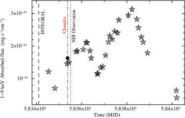
Figure 1: Lightcurve showing the absorbed 1–9 keV flux as determined by NICER observations (observation IDs 1200310101–1200310137). Times of the INTEGRAL discovery and our Chandra and NIR observations are also highlighted.

An examination of archival Neil Gehrels Swift data showed that the initial brightening of IGR J17591$-$2342 occurred as early as 2018 July 22 (MJD 58321) and peaked on 2018 July 25, predating the INTEGRAL discovery (Krimm, 2018). Further INTEGRAL observations post initial discovery showed a rebrightening of the source on 2018 August 30–31 (Sanchez-Fernandez et al., 2018; Kuiper et al., 2018). In Figure 1 we show the IGR J17591$-$2342 lightcurve for the absorbed 1-9 keV flux as determined by our analyses of NICER (Gendreau et al., 2016) observations (observation IDs 12000310101–1200310137; see §2.2 and §3.4 below). The two peaks shown in Figure 1 occur past at least one earlier peak in the lightcurve (Krimm, 2018), indicating a complex lightcurve. (The degree to which there is further substructure in the lightcurve over the July/August time frame is difficult to assess, owing to the disparate bandpasses of the various instruments with which IGR J17591$-$2342 was observed.)

IGR J17591$-$2342 is the $\mathrm{22^{nd}}$ member of the AMXP class. A high resolution X-ray spectroscopic characterization of this system and its surrounding matter may yield insights as to the evolution of millisecond pulsars from their accreting low-mass X-ray binary progenitors. In this paper, we discuss in detail the Chandra-HETGS spectra referenced by Nowak et al. (2018). We present evidence of an ionized outflow with velocity of order 1% the speed of light, and attempt to discern local and interstellar absorption. Taking the NICER observations used to create the lightcurve in Figure 1, we model the spectra that were strictly simultaneous with our Chandra observation, and discuss the differences in the model fits that are related to the different fields of view of these two instruments. We use INTEGRAL observations to discuss the spectra of IGR J17591$-$2342 above 10 keV. We also present new NIR observations, and discuss their implications.

2 Observations

Here we describe observations of IGR J17591$-$2342 performed in several different energy bands with a variety of instruments. Although the primary discovery was obtained by INTEGRAL (§1), our main focus will be observations obtained with Chandra (§2.1) and the Neutron star Interior Composition Explorer (NICER; §2.2) observatories. After describing the observations performed with Chandra and NICER, we briefly describe observations obtained with INTEGRAL (§2.3) and discuss our follow up optical and IR observations (§2.4).

2.1 Chandra-HETGS Observations

The HETGS consists of two sets of gratings, the High Energy Gratings (HEG, with bandpass $\approx 0.7$–9 keV and spectral resolution $E/\Delta E\approx 1\,300$ at 1 keV) and the Medium Energy Gratings (MEG, with bandpass $\approx 0.5$–8 keV and spectral resolution $E/\Delta E\approx 700$ at 1 keV), each of which disperses spectra into positive and negative orders. Here we consider only $\pm 1^{\rm st}$ order spectra of the HEG and MEG. There are too few counts to produce usable spectra from the higher spectral orders, while the undispersed $\mathrm{0^{th}}$ order spectra suffers from pileup. The first order spectra do not suffer from pileup, as the peak pileup fraction (in MEG $-1$ order near 3.8 keV where the count rate peaks at $\approx 0.13\,\mathrm{cts\,s^{-1}}\,\mbox{\AA}^{-1}$) is $\mathrel{\hbox to0.0pt{\raise 2.20013pt\hbox{$<$}\hss}{\lower 2.20013pt\hbox{$\sim$}}}0.5$%, and is significantly less for most other orders and wavelengths. (See Hanke et al. 2009.)

Our 20 ks Chandra data were processed using the suite of analysis scripts available as part of the Transmission Gratings Catalog (TGcat; Huenemoerder et al., 2011), running tools from CIAO v. 4.10 utilizing Chandra Calibration Database (CALDB) v. 4.7.8. The location of the center of the point source’s $0^{\rm th}$ order image was determined by intersecting the dispersion arms via the findzo tool. This is the position reported by Nowak et al. (2018). Its $0.6^{\prime\prime}$ accuracy (90% confidence) is that of the Chandra aspect solution when no other sources are within the field of view to further refine the astrometry.

Events within a 16 pixel radius of the above position were were assigned to $0^{\rm th}$ order. This position also defined the location of the dispersed HEG and MEG spectra. Any events that fell within $\pm 16$ pixels of the cross dispersion direction of either the HEG or MEG spectra were assigned to that grating arm using the tg_create_mask tool. Spectra were then created with events that fell within $\pm 3$ pixels of the cross-dispersion direction of the HEG and MEG arm locations (tg_extract), and assigned to a given spectral order with tg_resolve_events using the default settings. Spectral response matrices were created with the standard tools (fullgarf and mkgrmf).

2.2 NICER Observations

A series of observations with NICER were performed throughout the outburst of IGR J17591$-$2342 (see Sanna et al. 2018 and Figure 1). A total of 2.64 ks were strictly simultaneous with our 20 ks Chandra-HETGS observations. We consider only these data for purposes of spectral fitting. There are more NICER pointings, likely having a very similar spectral shape and flux, from periods shortly before or after the datasets that we consider. Our spectra, however, are already near the limits of the current understanding of systematic uncertainties in the NICER instrumental responses, and therefore inclusion of additional data would not improve our understanding of the NICER spectra.

The spectra were extracted using the NICER tools available in the Heasoft v6.25 package, using calibration products current as of the release of 2018 November 5. The response files were ni_xrcall_onaxis_v1.02.arf and nicer_v1.02.rmf, which we obtained directly from the NICER instrument team. We created a background file from NICER observations (with 66 ks of effective exposure) of a blank sky field previously observed by the Rossi X-ray Timing Explorer (RXTE). In all of the fits described below, rather than include a scaled version of these data as part of the spectral fit (i.e., “background subtraction”, even though what one is doing in ISIS is essentially adding these scaled background data to the model fits and comparing to the total observed data), we model the background spectra with a power law (with energy index $\Gamma\approx 0.78\pm 0.02$) and a broad gaussian feature centered on an energy of $(1.73\pm 0.07)$ keV with width $\sigma\approx(0.3\pm 0.1)$ keV. This model is fit to the background data, while simultaneously incorporating it into the source data model (without folding it through the spectral response, and appropriately scaling it for the $\approx 0.04$ relative exposure time of the source and background).

We bin the NICER spectra by a minimum of three spectral channels between 1–6 keV and four spectral channels between 6–9 keV. This approach ensures that our binning is approximately half width half maximum of the NICER spectral resolution (as determined from empirical measurements of delta functions forward folded through the NICER spectral response). Furthermore, we also impose a signal-to-noise minimum of 4; however, this latter criterion only affects the binning of the last few channels in the 8–9 keV range.

2.3 INTEGRAL Observations

In order to better understand the long-term behavior of IGR J17591$-$2342 at energies above 10 keV, we use INTEGRAL (Winkler et al., 2003, 2011) to study its high energy spectra. We analyzed all the available IBIS/ISGRI data of the monitoring observations starting from 2018 July 1 (MJD 58300; i.e., prior to the 2018 July 22 detection with archival data by Krimm 2018) up to 2018 October 23 (MJD 58414). Pointings (“science windows” in INTEGRAL parlance) that had the source within the IBIS/ISGRI field of view ($<$15^∘) and with integrated good times $>$1 000 s were used. This resulted in a total of 468 pointings of about 1 ks each (none of which were strictly simultaneous with our Chandra data). We analyzed the data using the Off-line Scientific Analysis (OSA) version 11 and the latest instrument characteristic files (2018 November).

Figure 2: IBIS/ISGRI 25–80 keV lightcurve of the hard X-ray brightest part of the outburst of IGR J17591$-$2342 (single pointing detections).

IGR J17591$-$2342 was detected in 22 pointings in the 25–80 keV band. In all these pointings, the source was within ${\sim}9^{\circ}$ from the center of the field of view. Figure 2 shows the lightcurve when the source is detected at a pointing level. As can be seen with respect to Figure 1, the detections overlap with the highest intensity periods from the NICER observations. The 25–80 keV source flux was obtained using a $\Gamma=2$ powerlaw spectrum (see §3.1).

2.4 Optical/IR Observations

For optical followup, we triggered optical to infrared observations of IGR J17591$-$2342 at the European Organisation for Astronomical Research in the Southern Hemisphere (ESO) of, using the VLT X-shooter instrument, a large-band UVB to NIR spectrograph, mounted on the UT2 Cassegrain focus (Vernet et al., 2011).

We obtained an I-band acquisition image on 25 August 2018, UTC 03h30 (exposure time 120 s). Figure 3 shows this finding chart of IGR J17591$-$2342 in the I-band, as acquired by X-shooter, indicating the Swift-XRT, Chandra, ATCA, and VLT/HAWK-I localization circles referenced in §1. From the image we derive a lower limit for the I-magnitude of the counterpart of the X-ray source of $\mathrm{I}\geq 24.7\pm 0.6$ mag (Johnson filter, magnitude of the source at $3\,\sigma$ above the sky noise). The uncertainty on the determined magnitude is rather large because we used a mean zero-point to flux-calibrate the photometry. This value in I-band is consistent with the H and Ks values obtained with HAWK-I observations (Shaw et al., 2018).

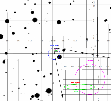
Figure 3: The finding chart of IGR J17591$-$2342 in the I-band, as acquired by X-shooter, indicating the Swift-XRT, Chandra, ATCA, and VLT/HAWK-I localization circles.

We also obtained NIR spectra on 25 August 2018, UT03h33 to UT04h37 (exposure time of 64 m, with airmass between 1.346–1.836) that we analyzed by performing a standard reduction using the esoreflex pipeline (Freudling et al., 2013). We detect a very faint spectrum ($\mathrm{S}/\mathrm{N}\sim 3.2$ at the maximum of the whole band coverage), as expected for a faint source with the I, H, and Ks band values discussed above. By flux-calibrating the faint spectrum, we find $\mathrm{F_{\nu}<0.12}$ mJy at the K-band wavelength of 2.2 $\mu$m (i.e., corresponding to K$>16.8$ mag). By applying a median filter we detect a faint continuum signal at the level of $\mathrm{F_{\nu}=0.025}$ mJy (i.e., K$=18.6$). Both measurements are consistent with the Ks value obtained with HAWK-I observation.

We point out here that in absence of detection of variability of the NIR candidate counterpart, we can not unambiguously associate either the candidate counterpart claimed by Shaw et al. (2018), nor the faint spectrum we detected with X-shooter, to the variable X-ray source.

For the value of the equivalent neutral absorption column, $N_{\mathrm{H}}=(4.9\pm 0.2)\times 10^{22}\,\mathrm{cm^{-2}}$, that we originally reported (Nowak et al. 2018; where we used the absorption model, cross sections, interstellar medium abundances discussed by Wilms et al. 2000), the corresponding V-band absorption is $\mathrm{Av\approx 24.6\,mag}$ (using the relationship between equivalent neutral column and V-band absorption given by Predehl & Schmitt 1995a; although see our more detailed discussions of absorption modeling below) and the K-band absorption is $\mathrm{Ak\approx 2.77}$ mag (using Fitzpatrick 1999).

The I$-$K color value being greater than at least 6 mag suggests a late spectral type companion star, located at the distance of the Galactic bulge.

3 Spectral Fits

3.1 Hard X-ray Continuum Fits

We first consider the IBIS/ISGRI spectra obtained from the average of the 22 pointings discussed above (i.e., the observations represented in the lightcurve shown in Figure 2). We fit these spectra with XSPEC v12.9.1 (Arnaud, 1996) using a powerlaw, and found a spectrum with $\Gamma$=$2.0\pm 0.2$ (reduced $\chi^{2}=1.29$, 10 degrees of freedom). These INTEGRAL observations extend the bandpass beyond the $\approx 70$ keV upper limit of NuSTAR observations, and here we find that IGR J17591$-$2342 is detected up to about 110 keV with no improvement obtained with the addition of a cutoff, even going out to $\approx 200$ keV (Figure 4, top panel).

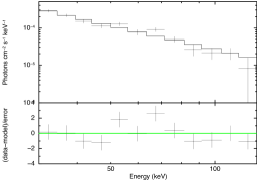
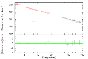
Figure 4: INTEGRAL spectra of IGR J17591$-$2342. Top panel: IBIS/ISGRI average spectrum and best fit of the data points shown in Figure 2 (effective exposure $\sim$24 ks). Bottom panel: simultaneous JEM-X (red) and IBIS/ISGRI (black) spectrum and best fit of five pointings with the source within the JEM-X fully coded field of view (effective exposure $\sim$6 ks with IBIS/ISGRI and $\sim$8 ks with JEM-X). See text.

We selected five pointings for which IGR J17591$-$2342 was both bright (second peak from Figure 1, between MJD 58380–58383) and within the JEM-X fully coded field of view (where the detection significance is maximum, $<3^{\circ}$). This selection resulted in a sub-sample of five science windows (ID: 200100250010, 200100340010, 200200250010, 200200330010, 200200340010). The simultaneous IBIS/ISGRI and JEM-X spectra of the five average pointings (Figure 4, bottom panel) resulted in a best fit (reduced $\chi^{2}=0.66$, 19 degrees of freedom) powerlaw spectrum with $\Gamma=1.8\pm 0.2$ and frozen neutral hydrogen N${}_{H}=3.3\times 10^{22}\,\mathrm{cm}^{-2}$ (taken from model E in Table 3, as discussed below in §3.2). Again, no cutoff is required within the INTEGRAL band. The average absorbed fluxes are $\mathrm{F_{25-80\,keV}}=4.7\times 10^{-10}\,\mathrm{erg\,cm^{-2}\,s^{-1}}$, $\mathrm{F_{3-25\,keV}}=5.4\times 10^{-10}\,\mathrm{erg\,cm^{-2}\,s^{-1}}$, and $\mathrm{F_{1-9\,keV}}=2.8\times 10^{-10}\,\mathrm{erg\,cm^{-2}\,s^{-1}}$. These values are compatible with the NICER fluxes shown in Figure 1. Assuming a distance of 8 kpc, they correspond to luminosities of $\mathrm{L_{25-80\,keV}}=3.6\times 10^{36}\,\mathrm{erg\,s^{-1}}$, $\mathrm{L_{3-25\,keV}}=4.1\times 10^{36}\,\mathrm{erg\,s^{-1}}$, and $\mathrm{L_{1-9\,keV}}=2.1\times 10^{36}\,\mathrm{erg\,s^{-1}}$.

A deeper analysis of the INTEGRAL data (mosaicking detections, spectral variability and timing) is beyond the scope of this paper.

3.2 Soft X-ray Continuum and Line Fits

All further analyses presented below were performed with the Interactive Spectral Interpretation System (ISIS; Houck & Denicola 2000). In order to increase the signal-to-noise ratio of our spectra, we combine the positive and negative first order HEG and MEG spectra using the ISIS functions match_dataset_grids (to match the HEG wavelength grid to that of MEG) and combine_datasets. We limit the energy range to 1–9 keV, but do not further bin the data, and use Cash (1979) statistics in the fits so as to facilitate the spectral line search, without biasing against absorption lines (see below).

We use a continuum model similar to the one Sanna et al. (2018) employed to fit joint NICER/NuSTAR data of IGR J17591$-$2342, specifically an absorbed (tbvarabs; Wilms et al. 2000, where we have also adopted the atomic cross sections and interstellar medium abundances discussed in that work) blackbody (bbodyrad) plus Comptonization (nthcomp; Życki et al. 1999) spectrum. Lacking simultaneous data above 9 keV, we do not have good leverage on some of the Comptonization parameters, so for all models we fix the coronal temperature to the 22 keV value found by Sanna et al. (2018) such that we can more readily compare to their findings. Our results in the 1–9 keV band are not sensitive to the coronal temperature; however, we note that a 22 keV coronal temperature would imply a spectral curvature in the 50–150 keV band that we do not see in the INTEGRAL spectra shown in Figure 4. The remaining nthcomp parameters are the normalization ($\mathrm{N_{nc}}$), the Compton powerlaw photon index ($\mathrm{\Gamma_{nc}}$), and the seed photon temperature ($\mathrm{kT_{nc}}$). The latter is tied to the blackbody temperature. The remaining bbodyrad parameter is its normalization, $\mathrm{N_{bb}}$, which nominally corresponds to $\mathrm{R^{2}_{km}/D^{2}_{10\,kpc}}$, where $\mathrm{R_{km}}$ is the source radius in km, and $\mathrm{D_{10\,kpc}}$ is the source distance in units of 10 kpc.

We include one other component in our model, not found in the NICER modeling of Sanna et al. (2018), namely a dust scattering component using the dustscat model (Baganoff et al., 2003). This component accounts for the scattering of soft X-rays out of our line of sight due to dust grains (see the discussion of Corrales et al. 2016). Taking this effect into account is important for the high spatial resolution measurements done with Chandra, which resolve IGR J17591$-$2342 into a point source and an arcminute size dust scattering halo. In contrast, as we further discuss below, the halo emission is included in the overall NICER spectrum owing to the arcminute scale resolution line of sight provided by this instrument. Following Nowak et al. (2012), in our Chandra analysis we therefore tie the halo optical depth to a value of $\tau_{scat}=0.324\,(N_{\mathrm{H}}/10^{22}\,\mathrm{cm^{-2}})$, where $N_{\mathrm{H}}$ is the equivalent neutral column obtained from the tbvarabs model. The dust halo size relative to the instrumental point spread function (PSF) is frozen at $\mathrm{H_{size}}=200$ (i.e., nearly all scattered photons are lost).

Our continuum model with the dust scattering halo describes the HETG spectra well (Cash statistic = 2048.6 for 2200 degrees of freedom), with a fitted equivalent neutral hydrogen column of $N_{\mathrm{H}}=(4.4\pm 0.2)\times 10^{22}\,\mathrm{cm^{-2}}$. The modeled 1–9 keV absorbed flux is $1.58\times 10^{-10}\,\mathrm{erg\,cm^{-2}\,s^{-1}}$. (All implied 1–9 keV absorbed fluxes for the models discussed below fall within a few percent of this value for the Chandra-HETGS spectra.) Assuming a distance of 8 kpc, this translates to an absorbed, isotropic luminosity in the 1–9 keV band of $1.21\times 10^{36}\,\mathrm{erg\,cm^{-2}\,s^{-1}}$

There are a number of prominent, narrow residuals in the spectra, especially near the Si edge region. To assess these residuals, we perform a “blind line search” (see the description of this functionality in Nowak 2017). We write our model (using ISIS notation) as follows:

$$\mathtt{tbvarabs*powerlaw} * \mathtt{exp(lines/bin\_width\_en)}$$ (1)

$$+0 * (\mathtt{constant}+...)~{}~{},$$

where $\mathtt{tbvarabs}$ is the Wilms et al. (2000) absorption model, $\mathtt{powerlaw}$ is the standard function with photon energy index $\Gamma$, $\mathtt{exp}$ is an exponential function, and $\mathtt{bin\_width\_en}$ is a function that returns the width of a data spectral bin in keV. The function $\mathtt{lines}$ is defined within the search script and returns a sum of standard $\mathtt{gaussian}$ fit functions, which as defined in ISIS or XSPEC are line profiles integrated within each data bin. It is for this latter reason that we divide by the data bin widths, so that any rebinning of the data will not strongly affect the fit parameters. We multiply the continuum by line functions within an exponential to ensure that the model never yields negative counts and so that it can smoothly pass from absorption to emission lines. The (multiple) $\mathtt{constant}$ functions (multiplied by 0 so as not to add to the continuum) are used as “dummy parameters” to allow us to transform the parameters of the $\mathtt{gaussian}$ line functions. Rather than fit a line amplitude, we instead fit a parameter closer to line equivalent width. Further, as a line becomes significantly more absorbed, we increase its equivalent width by increasing the line width, rather than by increasing the magnitude of the line amplitude. Since the data are not good enough to distinguish between being on the damping wings of the equivalent width curve of growth and a true increase in line width, we find that increasing the line width is numerically more stable. We limit all line widths to lie between values $\sigma=0.1$–20 eV.

In the line search procedure, we add an additional $\mathtt{gaussian}$ function to the $\mathtt{lines}$ function, and while holding the continuum and any previously detected lines fixed, we fit the parameters of this added line feature allowing its amplitude, width, and energy (within a limited range) to be free parameters. We store the change in fit statistics and the parameters of the fitted line. We scan along the full energy range of the spectra in this manner. The ten features with the largest change in fit statistic are then individually refit, now with both the continuum parameters and previous line fits allowed to vary. The feature leading to the largest improvement in fit statistic is then added to the model, and the scan is repeated. (At this stage, no error bars are determined for the line fits.)

Results for the eleven most significant features found by this method are presented in Table 1. Possible line identifications are also presented, along with the line redshifts if these identifications are in fact correct. These features were found in fits to the combined spectra; however, we visually inspected the combined fits applied to the spectra from the individual gratings arms, as well as applied to the spectra for just the combination of the HEG spectra and just the combination of the MEG spectra. The fitted features were consistent with these individual spectra, albeit with noisier statistics. None of the features appeared to be the result of a single spectrum or a single combination of spectra, as might be the case for an interloping faint source coincident with one gratings arm, or an unmodeled response feature limited to a subset of the arms.

Several significant features are found near the location of the expected Si absorption K-edge, so we include these in subsequent models, constraining the line energies to lie within a 10 eV interval and to have widths $\sigma<10$ eV. The possible blueshifted Si XIII Ly$\alpha$ feature (see Hell et al. 2016 for the most recent measurements of its energy) is fairly significant, so we include it in all subsequent fits, and further add Si XIII $\beta$ and $\gamma$ lines tied to the same blueshift and relative line width. Likewise, we include both the Si K$\alpha$ line at 1.7349 keV (whether this is a real feature, or an unmodeled component in the HETG response function) and the 1.848 keV feature near the Si edge (see discussion below). Although we have no good identification for the absorption feature near 1.695 keV, its presence may affect our models of the Si edge. We also include this feature in all subsequent models.

The possible presence of Ca features is somewhat unusual, but many of these features are formally more statistically significant than, e.g., the possible Si K$\alpha$ absorption line. Given that they may provide some information about the nature of an evolved companion, we include them in all subsequent fits constraining their line energies to lie within a 50 eV interval and to have widths $\sigma<20$ eV. They do not strongly influence any of the continuum or absorption parameters, as verified by Markov Chain Monte Carlo error contours for all models and parameters discussed below. We do not attempt to tie these features to a single common Doppler shift.

Lacking any plausible identification for the 1.009 keV or 3.47 keV features, we do not include them in subsequent models. The former feature consists of only a few events in a very faint portion of the observed spectrum (hence its large equivalent width, despite being only a few detected events). The latter feature does not strongly influence the remaining fit parameters.

Table 1: Results of Blind Line Search

$E_{obs}$	$\Delta C$	EW	Order	ID	$z$
keV		eV
1.0088	$-12.8$	$98$	1	$\cdots$	$\cdots$
1.6949	$-9.3$	$-2.3$	3	$\cdots$	$\cdots$
1.7349	$-7.5$	$-2.1$	9	Si K$\alpha$	0.003
1.8481	$-8.4$	$-3.2$	6	Si near edge	$\cdots$
1.8825	$-23.3$	$-4.3$	0	Si XIIIr	-0.009
2.2181	$-8.4$	$-4.2$	4	Si XIIIb	-0.016
3.4727	$-8.2$	$5.3$	7	$\cdots$	$\cdots$
3.6865	$-9.3$	$-5.6$	2	Ca K$\alpha$	0.0004
3.8447	$-8.3$	$6.1$	5	Ca XIXi	0.010
3.8963	$-7.3$	$-6.4$	10	Ca XIXr	0.016
4.2955	$-7.9$	$4.8$	8	Ca XXa	0.044

Note. — Results from a blind search to the unbinned, combined Chandra-HETG spectra, using a model consisting of an absorbed/scattered Comptonized spectrum. The columns give the fitted energy of the line, the change in Cash statistic when including the line, the line equivalent width (negative values are absorption, positive are emission), the order in which the lines were added (numbers 0–10), a potential line ID, and an implied redshift (negative values for blueshifts) if this ID is correct.

The above model fits the data well with a Cash statistic of 1963.0 for 2172 degrees of freedom; however, it requires a fitted equivalent neutral column of $N_{\mathrm{H}}=(5.1^{+0.3}_{-0.1})$ $\times 10^{22}\,\mathrm{cm^{-2}}$. This value is somewhat larger than the $N_{\mathrm{H}}=(3.6\pm 1.1)$–$(4.4\pm 0.3)\times 10^{22}\,\mathrm{cm^{-2}}$ values found by Sanna et al. (2018) (Swift/NICER/ NuSTAR/INTEGRAL) and Russell et al. (2018b) (Swift), respectively. Our higher equivalent neutral column value is in part driven by the need to describe the complexities of the Si K-edge region, as well as possibly also by differences in the abundance sets used. We consider this region further in §3.3 below.

3.3 Si Edge Region Models

Recently, Schulz et al. (2016) have published a Chandra-HETGS study of the Si K-edge region of Galactic X-ray binaries with (continuum) fitted equivalent neutral columns in the range of $N_{\mathrm{H}}\approx(1-6)\times 10^{22}\,\mathrm{cm^{-2}}$. Among the conclusions of this survey are the following: 1) the absorption model of Wilms et al. (2000), when using their adopted interstellar medium (ISM) abundances, under predicts the depth of the Si K-edge, 2) the edge itself is complex, 3) there often is a near-edge absorption feature at $\approx 1.849$ keV that even in a single source appears to have a variable equivalent width that is loosely correlated with fitted $N_{\mathrm{H}}$, and 4) there often is a Si XIII absorption feature also with variable equivalent width with an even weaker correlation with fitted $N_{\mathrm{H}}$. The variability of the latter two features indicates that for many of the eleven X-ray binaries included in the survey of Schulz et al. (2016), some fraction of the observed absorption is local to the system, as opposed to being more broadly distributed throughout the ISM.

The near edge and Si XIII features are already accounted for in our models. The energy of the near edge feature is consistent with the values found by Schulz et al. (2016), and therefore this feature is likely “at rest” relative to its expected energy. On the other hand, we do not find Si XIII at rest but instead find a blueshifted velocity of $\mathrm{\approx 2\,800\,km\,s^{-1}}$ with $\mathrm{\sigma\approx 200\,km\,s^{-1}}$. This is in contrast to Schulz et al. (2016) who found the magnitude of any red or blueshifts to be $\mathrm{\mathrel{\hbox to0.0pt{\raise 2.20013pt\hbox{$<$}\hss}{\lower 2.20013pt\hbox{$\sim$}}}200\,km\,s^{-1}}$, but found velocity widths on the order of $\mathrm{\mathrel{\hbox to0.0pt{\raise 2.20013pt\hbox{$<$}\hss}{\lower 2.20013pt\hbox{$\sim$}}}700\,km\,s^{-1}}$.

To further compare with the phenomenological models of Schulz et al. (2016), we take the continuum models of §3.2 and modify the tbvarabs Si edge by either reducing the Si abundance to 0.01 of the ISM value and adding a phenomenological edge model (with parameters $\mathrm{E_{edge}}$ and $\mathrm{\tau_{edge}}$), or by instead allowing the Si abundance ($\mathrm{A_{Si}}$) to be a free parameter. These models are referred to as models A and B, respectively, in Table 3, and the flux corrected spectra in the Si edge region are shown in the top two panels of Figure 5. For both models, the equivalent neutral column is reduced to a value of $N_{\mathrm{H}}\approx 4.2\times 10^{22}\,\mathrm{cm^{-2}}$, with either the abundance increasing to a value of $\mathrm{A_{Si}=1.76^{+0.49}_{-0.46}}$, or the phenomenological edge requiring an optical depth of $\mathrm{\tau_{edge}=0.19\pm 0.05}$. Both of these results are completely consistent with those found by Schulz et al. (2016), with the value of the added edge optical depth relative to fitted equivalent neutral column falling within the data range shown in their Figure 5. The Schulz et al. (2016) results also indicate edge optical depth values approximately twice that predicted by the Wilms et al. (2000) model, consistent with our findings for the fitted abundance in our model B. We note, however, that the magnitude of our fitted value for the equivalent width of the near edge feature is $\approx 50$% larger than the largest values found by Schulz et al. (2016). We further discuss this result below.

Also as discussed by Schulz et al. (2016), the location of the edge has a degree of uncertainty due to the presence of the near edge absorption feature. In fact, our best fit edge energy is higher than the absorption feature energy, although the error bars allow for the edge to be at 1.844 keV which is the expected location for neutral Si at rest.

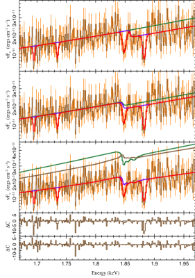
Figure 5: The silicon K-edge region for the flux-corrected combined HEG and MEG first order Chandra-HETG spectra (brown with orange 1 $\sigma$ error bars), fit with an absorbed Comptonized spectrum (see §3.2). In all panels the red line shows the full fitted model, and the purple line shows the model with the absorption lines removed. In the top panel, a phenomenological edge has been used to describe the Si K-edge (model A). The green line shows the model with edge and lines removed. In the second panel, the Si K-edge absorption has been modeled by allowing a freely variable (increased) Si abundance in the ISM (model B). The green line shows the model with the Si abundance set to the solar value and the lines removed. The third panel shows the model using the dust scattering and absorption models of Corrales et al. (2016) (model C). The green line shows the model with only the dust absorption contribution. The brown line shows the model with only the dust scattering contributions. The fourth panel shows the residuals for model C with the lines removed. The fifth panel shows the residuals for model C.

We next consider a more physical model for the edge region. Specifically, we use the dust scattering and edge models of Corrales et al. (2016), which in their ISIS implementations are broken up into individual absorption and scattering components for both silicate and graphite dust grains. We multiply the scattering components by an energy-dependent factor in an identical manner as for the dustscat model (Baganoff et al., 2003) to account for the fraction of flux that scatters back into our line of sight given the finite size of the instrumental PSF. We again parameterize this factor with a fixed value of $\mathrm{H_{size}=200}$ (i.e., nearly all scattered photons are lost from the spectrum). We further tie the dust components to the fitted equivalent neutral column via two parameters: the mass fraction of the ISM column in dust ($\mathrm{f_{dust}})$, and the fraction of dust in silicates $\mathrm{f_{silicate}}$. We fit one model where these values are free parameters (model C), and one model where they are frozen to their commonly presumed values (see Corrales et al. 2016) of $\mathrm{f_{dust}=0.01}$ and $\mathrm{f_{silicate}=0.6}$ (model D). Both models fit the data extremely well, as seen in Figure 5 and Table 3.

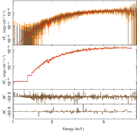
Figure 6: The flux-corrected combined HEG and MEG first order Chandra-HETG spectra (brown with orange 1 $\sigma$ error bars), fit in the 1–9 keV band with an absorbed and scattered Comptonized spectrum (model C; see §3.3). Top panel: combined spectrum, with one MEG channel per bin. Second panel: spectrum rebinned to a S/N$\geq 5$ and $\geq 4$ MEG channels per bin, without refitting the spectrum. Third/fourth panels: Cash statistic residuals for the spectral binnings and fit shown in the first two panels.

We show the fit for model C in Figure 6. The inclusion of scattering and solid state absorption effects due to dust grains reduces the overall required column to a value of $N_{\mathrm{H}}\approx(2.9\pm 0.5)\times 10^{22}\,\mathrm{cm^{-2}}$. The presence of a near edge absorption feature is still required. We note that in terms of equivalent width all of the models discussed above have comparable values, despite obvious changes in the absolute line depth as seen in Figure 5. This is because the equivalent width is a relative measure, and what is being deemed as “continuum” in the equivalent width calculations includes the edge from the absorption/scattering models.

Table 2: MCMC Line Significances

abs	Si K$\alpha$	near edge	Si XIIIa	Si XIIIb	Si XIIIg	Ca K$\alpha$	Ca XIXi	Ca XIXr	Ca XXa
96.9%	66.3%	95.4%	99.999%	64.3%	95.9%	99.4%	99.1%	99.7%	97.0%

Note. — Significances from a Markov Chain Monte Carlo (MCMC) analysis of model C, subject to the line constraints discussed in the text. Labels are the same as in Table 3. Percentages are the fraction of the posterior probability that is $<0$ for absorption lines and $>0$ for emission lines. Significances do not include multiplicity of trials.

We use model C, which has the most freedom to fit the Si edge region with the neutral absorption and dust scattering models, to assess the significances of the lines beyond the nominal 90% confidence intervals presented in Table 3. We use this model in a Markov Chain Monte Carlo (MCMC) calculation implemented in ISIS following the prescription of Goodman & Weare (2010). (See our detailed descriptions in Murphy & Nowak 2015.) We evolve a set of 320 “walkers” (ten initial models per free parameter, with their initial parameters randomly distributed over the central 3% of the 90% confidence intervals) for 40 000 steps, of which we only retain the last 2/3 for assessing probabilities (yielding over 8.5 million samples in our posterior probability distributions). The line widths and energies are constrained as discussed above.

We calculate line significances as the fraction of the posterior probability distribution with negative line amplitudes for absorption lines, or the fraction of the posterior probability distribution with positive amplitudes for emission lines. This is of course a somewhat local and constrained probability distribution that does not account for any “multiplicity of trials” in our initial assessment of lines to include in our models. We present these line significances in Table 2. In general, these significances are commensurate with the results of the 90% confidence intervals presented in Table 3, with the blueshifted Si XIII resonance line being the most significant feature. The Si K$\alpha$ line is less significant than one might expect from Table 3 owing to the fact that if the line energy shifts from the best fit value by more than $\approx 5$ eV in either direction, a broader weak emission feature is allowed.

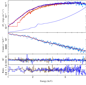
Figure 7: Top panel: The flux-corrected combined HEG and MEG first order Chandra-HETG spectra (brown histogram) and NICER spectra (blue circles, pale blue histogram is the background model), jointly fit with an absorbed and scattered blackbody plus Comptonization model (model E). Owing to the different fields of view of each instrument, the dust scattering component is different in the Chandra and NICER spectra, and accounts for the deviation between the two spectra at energies $\mathrel{\hbox to0.0pt{\raise 2.20013pt\hbox{$<$}\hss}{\lower 2.20013pt\hbox{$\sim$}}}3$ keV. The NICER spectra also have been renormalized to account for a fitted cross normalization constant between the Chandra-HETGS and NICER spectra. The second panel shows the simultaneous fit to the background spectra (see text). The third and fourth panels show the residuals for the model fit. The third panels shows the Cash statistics residuals for the Chandra-HETGS (brown histogram) and NICER source (blue histogram) and background (light blue histogram) spectra at the binning of the fit (see text). The fourth panel shows the the data/model ratio residuals, but now omitting the NICER background spectra and with the Chandra-HETGS spectra rebinned for clarity, but without refitting the model.

3.4 Joint Fits with NICER Spectra

We next consider models C and D, but with the inclusion of 1–9 keV NICER spectra. The NICER instrument has a field of view $\approx 30$ square arcmin, i.e., an $\approx 3$′ radius (Gendreau et al., 2016). We therefore expect a large fraction of the dust scattered photons, lost from the Chandra-HETGS spectra, to scatter back into the field of view of NICER (see the discussion of Corrales et al. 2016). Although these scattered photons are time-delayed (McCray et al., 1984), there is no indication that the spectrum from tens of thousands of seconds earlier was substantially different from what we observed. As expected, fitting for the size of the dust scattering halo relative to the NICER PSF, we find $\mathrm{H_{size}<1.9}$. (We set the lower bound of $\mathrm{H_{size}=0.01}$.) That is, the spectra are consistent with a substantial fraction (nearly all) of the scattered X-rays returning to the NICER field of view. This is in fact apparent when comparing the flux-corrected spectra between Chandra-HETGS and NICER, as seen in Figure 7.

Table 3: Spectral Fit Parameters

Parameter	Units	A	B	C	D	E	F
$N_{\mathrm{H}}$	$10^{22}\,\mathrm{cm^{-2}}$	${4.23}^{+0.16}_{-0.14}$	${4.21}^{+0.18}_{-0.15}$	${2.86}^{+0.54}_{-0.55}$	${2.62}^{+0.07}_{-0.07}$	${3.28}^{+0.10}_{-0.09}$	${2.63}^{+0.05}_{-0.21}$
$\mathrm{A_{Si}}$		$\cdots$	${1.76}^{+0.48}_{-0.47}$	$\cdots$	$\cdots$	$\cdots$	$\cdots$
$\mathrm{E_{edge}}$	keV	${1.859}^{+0.004}_{-0.020}$	$\cdots$	$\cdots$	$\cdots$	$\cdots$	$\cdots$
$\mathrm{\tau_{edge}}$		${0.19}^{+0.05}_{-0.05}$	$\cdots$	$\cdots$	$\cdots$	$\cdots$	$\cdots$
$\mathrm{f_{dust}}$	$10^{-2}$	$\cdots$	$\cdots$	${0.71}^{+0.60}_{-0.26}$	1	${0.49}^{+0.04}_{-0.04}$	1
$\mathrm{f_{silicate}}$		$\cdots$	$\cdots$	${0.92}^{+0.08}_{-0.49}$	0.6	${1.0}_{-0.06}$	0.6
$\mathrm{C_{n}}$		$\cdots$	$\cdots$	$\cdots$	$\cdots$	${0.83}^{+0.02}_{-0.02}$	${0.77}^{+0.01}_{-0.01}$
$\mathrm{H_{size}}$		$\cdots$	$\cdots$	$\cdots$	$\cdots$	${0.01}^{+1.33}_{-0.0}$	${1.85}^{+0.06}_{-0.06}$
$\mathrm{N_{nc}}$		${0.09}^{+0.01}_{-0.01}$	${0.09}^{+0.01}_{-0.01}$	${0.10}^{+0.02}_{-0.01}$	${0.10}^{+0.01}_{-0.01}$	${0.10}^{+0.01}_{-0.01}$	${0.09}^{+0.01}_{-0.01}$
$\mathrm{\Gamma_{nc}}$		${1.98}^{+0.06}_{-0.07}$	${1.99}^{+0.07}_{-0.07}$	${2.06}^{+0.08}_{-0.07}$	${2.05}^{+0.05}_{-0.05}$	${2.02}^{+0.04}_{-0.02}$	${1.96}^{+0.03}_{-0.03}$
$\mathrm{kT_{nc}}$	keV	${0.084}^{+0.003}_{-0.003}$	${0.082}^{+0.003}_{-0.002}$	0.06	0.06	${0.057}^{+0.001}_{-0.001}$	${0.074}^{+0.002}_{-0.007}$
$\mathrm{N_{bb}}$	$10^{7}$	${5.5}^{+1230}_{-5.2}$	${8.1}^{+630}_{-7.7}$	${330}^{+470}_{-270}$	${400}^{+390}_{-290}$	${2000}^{+3800}_{-1900}$	${30.7}^{+230}_{-22.2}$
$\mathrm{E_{abs}}$	keV	${1.6949}^{+0.0005}_{-0.0008}$	${1.6949}^{+0.0006}_{-0.0008}$	${1.6949}^{+0.0005}_{-0.0008}$	${1.6949}^{+0.0006}_{-0.0008}$	1.6949	1.6949
$\mathrm{\sigma_{abs}}$	eV	${0.2}^{+0.9}_{-0.1}$	${0.2}^{+0.9}_{-0.1}$	${0.2}^{+0.9}_{-0.1}$	${0.2}^{+0.9}_{-0.1}$	0.2	0.2
$\mathrm{EW_{abs}}$	eV	${-2.3}^{+1.1}_{-0.8}$	${-2.3}^{+0.9}_{-0.8}$	${-2.3}^{+0.6}_{-1.2}$	${-2.3}^{+0.9}_{-0.8}$	-2.3	-2.3
$\mathrm{E_{Si\,K\alpha}}$	keV	${1.735}^{+0.001}_{-0.001}$	${1.735}^{+0.001}_{-0.001}$	${1.735}^{+0.001}_{-0.001}$	${1.735}^{+0.001}_{-0.001}$	1.735	1.735
$\mathrm{\sigma_{Si\,K\alpha}}$	eV	${0.2}^{+1.3}_{-0.1}$	${0.3}^{+1.1}_{-0.2}$	${0.2}^{+1.3}_{-0.1}$	${0.2}^{+1.3}_{-0.1}$	0.2	0.2
$\mathrm{EW_{Si\,K\alpha}}$	eV	${-2.3}^{+1.1}_{-0.8}$	${-2.3}^{+1.2}_{-0.8}$	${-2.2}^{+0.4}_{-0.9}$	${-2.3}^{+1.2}_{-0.8}$	-2.2	-2.3
$\mathrm{E_{near\,edge}}$	keV	${1.848}^{+0.002}_{-0.001}$	${1.848}^{+0.002}_{-0.002}$	${1.848}^{+0.002}_{-0.003}$	${1.848}^{+0.002}_{-0.002}$	1.848	1.848
$\mathrm{\sigma_{near\,edge}}$	eV	${2.1}^{+2.1}_{-2.0}$	${1.6}^{+2.6}_{-1.5}$	${1.8}^{+3.0}_{-1.7}$	${1.8}^{+2.9}_{-1.7}$	1.8	1.8
$\mathrm{EW_{near\,edge}}$	eV	${-4.1}^{+2.0}_{-1.7}$	${-3.3}^{+1.5}_{-2.0}$	${-3.3}^{+2.2}_{-0.5}$	${-3.3}^{+2.4}_{-0.1}$	-3.3	-3.3
$\mathrm{z_{Si\,XIII}}$		${0.0093}^{+0.0006}_{-0.0009}$	${0.0093}^{+0.0006}_{-0.0010}$	${0.0092}^{+0.0007}_{-0.0008}$	${0.0092}^{+0.0006}_{-0.0008}$	0.0092	0.0092
$\mathrm{\sigma_{Si\,XIII}}$	eV	${1.5}^{+2.2}_{-1.2}$	${1.5}^{+2.3}_{-1.2}$	${1.7}^{+1.8}_{-1.4}$	${1.8}^{+1.9}_{-1.5}$	1.8	1.8
$\mathrm{EW_{Si\,XIIIa}}$	eV	${-4.3}^{+0.7}_{-1.7}$	${-4.4}^{+1.5}_{-1.8}$	${-4.7}^{+1.8}_{-1.5}$	${-4.7}^{+1.8}_{-1.6}$	-4.7	-4.7
$\mathrm{EW_{Si\,XIIIb}}$	eV	${-0.7}^{+2.9}_{-2.1}$	${-0.6}^{+2.8}_{-2.1}$	${-0.5}^{+2.9}_{-2.0}$	${-0.5}^{+2.9}_{-2.2}$	-0.5	-0.5
$\mathrm{EW_{Si\,XIIIg}}$	eV	${-2.3}^{+2.9}_{-3.3}$	${-2.3}^{+2.9}_{-3.3}$	${-2.4}^{+3.1}_{-3.0}$	${-2.4}^{+2.6}_{-3.1}$	-2.4	-2.4
$\mathrm{E_{Ca\,K\alpha}}$	keV	${3.687}^{+0.007}_{-0.006}$	${3.687}^{+0.007}_{-0.007}$	${3.687}^{+0.007}_{-0.006}$	${3.687}^{+0.007}_{-0.006}$	3.687	3.687
$\mathrm{\sigma_{Ca\,K\alpha}}$	eV	${4.3}^{+7.8}_{-4.2}$	${4.3}^{+7.8}_{-4.2}$	${4.4}^{+7.8}_{-4.3}$	${4.3}^{+7.8}_{-4.2}$	4.4	4.3
$\mathrm{EW_{Ca\,K\alpha}}$	eV	${-6.1}^{+3.2}_{-3.2}$	${-6.1}^{+3.2}_{-3.2}$	${-6.2}^{+3.8}_{-3.3}$	${-6.1}^{+3.2}_{-3.2}$	-6.2	-6.1
$\mathrm{E_{Ca\,XIXi}}$	keV	${3.845}^{+0.028}_{-0.014}$	${3.845}^{+0.027}_{-0.014}$	${3.845}^{+0.029}_{-0.015}$	${3.845}^{+0.027}_{-0.014}$	3.845	3.845
$\mathrm{\sigma_{Ca\,XIXi}}$	eV	${0.7}^{+19.3}_{-0.6}$	${1.1}^{+18.9}_{-1.0}$	${1.0}^{+19.0}_{-0.9}$	${0.6}^{+19.4}_{-0.5}$	1.0	0.6
$\mathrm{EW_{Ca\,XIXi}}$	eV	${6.1}^{+15.8}_{-3.5}$	${6.1}^{+15.5}_{-3.5}$	${6.0}^{+61.6}_{-3.6}$	${6.1}^{+29.2}_{-3.6}$	6.0	6.1
$\mathrm{E_{Ca\,XIXr}}$	keV	${3.896}^{+0.011}_{-0.008}$	${3.896}^{+0.011}_{-0.008}$	${3.896}^{+0.011}_{-0.008}$	${3.896}^{+0.011}_{-0.008}$	3.896	3.896
$\mathrm{\sigma_{Ca\,XIXr}}$	eV	${6.4}^{+12.8}_{-6.3}$	${6.4}^{+12.9}_{-6.3}$	${6.5}^{+13.0}_{-6.4}$	${6.4}^{+12.9}_{-6.3}$	6.5	6.4
$\mathrm{EW_{Ca\,XIXr}}$	eV	${-6.6}^{+3.9}_{-4.4}$	${-6.6}^{+3.9}_{-4.5}$	${-6.7}^{+4.0}_{-4.4}$	${-6.6}^{+3.9}_{-4.2}$	-6.7	-6.6
$\mathrm{E_{Ca\,XXa}}$	keV	${4.295}^{+0.007}_{-0.010}$	${4.295}^{+0.006}_{-0.009}$	${4.294}^{+0.007}_{-0.006}$	${4.296}^{+0.005}_{-0.011}$	4.294	4.294
$\mathrm{\sigma_{Ca\,XXa}}$	eV	${0.8}^{+1.3}_{-0.7}$	${0.2}^{+0.0}_{-0.1}$	${0.3}^{+2.7}_{-0.2}$	${0.3}^{+0.2}_{-0.2}$	0.5	0.3
$\mathrm{EW_{Ca\,XXa}}$	eV	${7.0}^{+5.3}_{-4.3}$	${6.9}^{+5.2}_{-4.2}$	${6.9}^{+1.1}_{-4.5}$	${6.8}^{+0.9}_{-4.2}$	6.9	6.8
Cash/DoF		1958.7/2170	1959.6/2171	1956.6/2171	1957.8/2173	2507.0/2645	2597.1/2647

Note. — All errors are 90% confidence level for one interesting parameter (determined as $\Delta$Cash=2.71, which is correct in the limit that Cash statistics approach $\chi^{2}$ statistics). Models A–D are for Chandra-HETG 1-9 keV spectra only, while models E and F also include NICER 1-9 keV spectra. Italicized parameters were held fixed at that value. See text for a description of the models and model parameters.

There are, however, significant residuals for the NICER spectra in the $\approx 1.5$–2.5 keV region. It is likely that both the fitted equivalent neutral column, as well as the fraction of mass in dust — and specifically the fraction of mass in silicate dust — is being partly driven by the systematic uncertainties in the NICER response functions. We have used MCMC analyses identically as described above for all of our model fits to determine the interdependencies of the fitted parameters, and to make confidence contours of these parameter correlations. Although the contours of equivalent neutral column vs. silicate dust mass column (Figure 8, left) are consistent between Chandra-HETGS and NICER, the small NICER spectra error bars, coupled with large fit ratio residuals, indicate that NICER systematics in this regime are still a significant concern for this aspect of the model fits.

To further bring agreement between the Chandra-HETGS and NICER spectra, we have to include a cross-normalization between the two detectors. We choose an energy-independent cross-normalization constant, with the only energy-dependent differences between the two observations being the above expected differences due to the dust scattering halo. Although such energy-dependent cross calibration differences may exist, we do not believe these data are sufficiently constraining so as to allow exploration of a more complicated model. For Model E, which allows the greatest freedom in the dust absorption and scattering parameters, we also find the largest cross-normalization constant, $0.83\pm 0.02$. This is somewhat lower than one might initially expect from the 1–9 keV NICER flux, which is $1.48\times 10^{-10}\,\mathrm{erg\,cm^{-2}\,s^{-1}}$ (see Figure 1). Note, however, that the NICER spectra are less affected by the dust halo, and therefore would have a slightly higher flux than Chandra-HETGS even if the cross normalization constant were unity.

In Figure 8 we show the dependence of this cross normalization constant on the fitted and/or presumed equivalent neutral and silicate dust mass columns. There are significant systematic dependencies upon the latter, which is not surprising given the ratio residuals present in Figure 7. For the models that we have explored, however, we have not found a cross normalization constant $\mathrel{\hbox to0.0pt{\raise 2.20013pt\hbox{$>$}\hss}{\lower 2.20013pt\hbox{$\sim$}}}0.85$.

4 Discussion

We have presented a series of fits to INTEGRAL, NICER, and Chandra-HETGS spectra of the AMXP IGR J17591$-$2342 together with on-source NIR observations performed within our collaboration.

4.1 Comparison with previous findings

Our IBIS/ISGRI spectrum of the brightest part of the hard X–ray outburst of IGR J17591$-$2342 (24 ks, Fig. 2) results in a non-attenuated power-law model ($\Gamma=2.0\pm 0.2$) with no cut-off required, and source detection up to about 110 keV. This is compatible with what was found in the dedicated INTEGRAL Target of Opportunity observations of the source (164 ks; Kuiper et al., 2018) that significantly detected IGR J17591$-$2342 up to 150 keV using a powerlaw model description. Such a high energy spectrum is representative for AMXPs that are known to have quite high Comptonizing plasma temperatures — of the order of several tens of keV (e.g., Falanga et al., 2013, and references therein), similar to the so-called Atoll LMXBs known to host NS.

In agreement with the many preliminary analyses presented in the references of §1, and specifically with the Swift/NICER/NuSTAR/INTEGRAL analyses presented by Sanna et al. (2018), we find that a highly absorbed powerlaw ($N_{\mathrm{H}}\approx 4\times 10^{22}\,\mathrm{cm^{-2}}$, $\Gamma\approx 2$) describes the spectra well. When specifically modeling the 1–9 keV spectra with a Comptonized blackbody, fixing the coronal temperature to the 22 keV employed by Sanna et al. (2018), there is an implied spectral curvature in the 50–150 keV INTEGRAL band that we do not detect. However, our 1–9 keV spectra are largely insensitive to the temperature of the corona, and instead are predominantly sensitive to the spectral slope of Compton continuum which is $\Gamma\approx 2$ for all the models that we have considered.

Our one major difference from the models of Sanna et al. (2018) is that we fit a lower temperature, and hence a larger normalization, for the seed photons input to Compton corona. They found a blackbody emission area consistent with the surface of a neutron star. In contrast, the blackbody normalizations presented in Table 3 imply emission radii ranging from $\approx 1\,000$–$200\,000$ km, if the source is at the 8 kpc distance of the Galactic bulge. This would imply that the seed photons for Comptonization were instead generated by the accretion flow onto the neutron star, rather than its surface.

A second difference between our model fit results and previous fit results using spectra from detectors with lower spectral resolution than for Chandra-HETGS concerns the fitted equivalent neutral column. Our model fits to $N_{\mathrm{H}}$ are not only driven by the curvature of the soft X-ray continuum spectra, but are also driven by direct modeling of X-ray absorption edges of various atomic species. The advent of the era of high resolution spectroscopy is among the factors that drove the development of the tbvarabs model (Wilms et al., 2000). This model utilizes improved knowledge of ISM abundances and atomic cross sections, and it also provides a more precise description of atomic edges from such species as O, Fe (via the L and K edges), Ne, and for the case of IGR J17591$-$2342, the Si edge. However, as pointed out by Schulz et al. (2016), the tbvarabs model under predicts the depth of the Si edge for a given equivalent neutral column. Phenomenologically, this can be accounted for by either adding a separate Si-region edge to the model (while artificially reducing the Si abundance) with $\mathrm{\tau_{edge}=0.19\pm 0.05}$, or by increasing the Si abundance in the model to $\mathrm{A_{Si}=1.76^{+0.48}_{-0.47}}$ (models A and B in Table 3). This is in complete agreement with the results of Schulz et al. (2016) and also with newer abundance measurements for B-stars in the Galaxy (Nieva & Przybilla, 2012), which imply $\mathrm{A_{Si}}=1.70$.

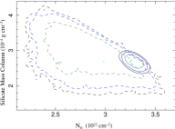
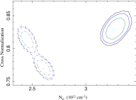
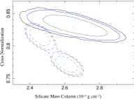
Figure 8: Contours for interstellar absorption and dust absorption and scattering parameters for absorbed/scattered blackbody plus Comptonization fits to the 1–9 keV Chandra-HETG spectra on their own (dashed contours— model C), or in combination with the 1–9 keV NICER spectrum (solid— model E — and dash-dot— model F — contours), as derived from Markov Chain Monte Carlo (MCMC) analyses of the model fits. Left: Equivalent hydrogen column for gas absorption vs. silicate mass column for dust scattering and absorption. Middle: Cross normalization value for the NICER spectrum (relative to Chandra-HETG normalization) vs. equivalent hydrogen column. Solid contours are for a freely variable dust mass and silicate fraction (see §3.3), while the dash-dot contours presume a fixed dust mass fraction of 0.01 and a fixed silicate fraction of 0.6. Right: NICER cross normalization constant vs. silicate mass column for both freely variable and fixed dust mass and silicate fractions.

4.2 Dust absorption/scattering and source distance

A more physical description of this result is provided by employing the models of Corrales et al. (2016). As pointed out by these authors, as an absorption model the tbvarabs model does not account for soft X-ray scattering or solid state absorption effects by dust except for shielding. Both are important for the high spatial resolution observations of Chandra-HETGS. Dust scatters X-rays out of our line of site on arcsec size scales, but it scatters back into the line of site, albeit with a time delay, on arcminute scales (McCray et al., 1984). Thus, we have to account for both dust scattering and solid state absorption effects in modeling the Chandra-HETGS spectra of IGR J17591$-$2342. We have done this in models C and D from Table 3, using the dust models of Corrales et al. (2016). The inclusion of dust has the effect of reducing the required equivalent neutral column. Since it contains the least restrictive assumptions about the column mass fraction in dust or the fraction of dust in silicates, we consider model C, with $N_{\mathrm{H}}=(2.9\pm 0.5)\times 10^{22}\,\mathrm{cm^{-2}}$, to be our most fair estimate for the equivalent neutral column along our line of site to IGR J17591$-$2342.

This value is lower, by $\approx 1/5$–1/3, compared to model estimates made without accounting for dust effects (e.g., Sanna et al. 2018; Russell et al. 2018b). As discussed by Russell et al. (2018b), the equivalent neutral column inferred from reddening maps is $N_{\mathrm{H}}<2.2\times 10^{22}\,\mathrm{cm^{-2}}$ (for the full column along the line of site), and is $N_{\mathrm{H}}>0.7\times 10^{22}\,\mathrm{cm^{-2}}$ for distances $>6$ kpc. Thus Russell et al. (2018b) argue for a large distance, at the Galactic bulge distance or beyond, and further argue that IGR J17591$-$2342 is radio bright for an AMXP. (In fact, based upon its radio brightness relative to its X-ray flux, IGR J17591$-$2342 was initially hypothesized to be a black hole candidate; Russell et al. 2018a.) Russell et al. (2018b) offer the alternative hypothesis that if much of the absorption is local to the system, then it can be significantly closer allowing for a more typical ratio of radio to X-ray luminosity for an AMXP. (Empirically, the radio flux drops more slowly than X-ray flux for decreasing luminosities.)

Although our inclusion of the dust effects lowers the fitted equivalent neutral column, it does not do so substantially enough to fundamentally alter the conclusions of Russell et al. (2018b).

A further argument in favor of the source being at a large distance with a column primarily attributable to the ISM (as opposed to local absorption) is the presence of substantial near edge absorption feature at an energy of 1.848 keV. Such a near edge absorption feature is routinely seen in X-ray binary sources with columns in the range of $\approx(1$–$\mathrm{8)\times 10^{22}\,cm^{-2}}$ (Schulz et al., 2016); however, the near edge feature is often variable and of lower equivalent width magnitude than we observe here. The speculation is that dust local to the system is destroyed/ionized by the source’s X-rays. Schulz et al. (2016) essentially fit a spectral model equivalent to model A in Table 3, and the highest magnitude equivalent widths they find are $\approx-8\pm 2$ mA for $N_{\mathrm{H}}\mathrel{\hbox to0.0pt{\raise 2.20013pt\hbox{$>$}\hss}{\lower 2.20013pt\hbox{$\sim$}}}4\times 10^{22}\,\mathrm{cm^{-2}}$. For IGR J17591$-$2342 fit with model A, we find $\mathrm{EW}=-4.1^{+2.0}_{-1.7}$ eV $=-16^{+8}_{-7}$ mA. If this feature were primarily local and subject to destruction by ionization due to the source, it would be unusual to find its equivalent width at a magnitude greater than observed in the entire Schulz et al. (2016) sample, while at the same time also seeing a Si XIII absorption line with a high magnitude equivalent width ($\mathrm{EW}=-4.3^{+0.7}_{-1.7}$ eV, $=-15^{+3}_{-6}$ mA for model A) outflowing at 0.0093 c. Thus we hypothesize that a large fraction of the observed column is associated with the ISM (as is consistent with our NIR results discussed in §2.4), the source is at a large distance, and hence its radio flux is indeed high for an AMXP.

4.3 Outflowing wind

The Si XIII absorption line indicates a mass outflow in the IGR J17591$-$2342 system. We can constrain the energy flux associated with this outflow based upon the line equivalent width. Assuming that the line is on the linear part of the curve of growth, $\mathrm{W_{\lambda}}$, its equivalent width in Å, is related to the Si XIII column, $\mathrm{N_{Si13}}$, by

$$\mathrm{\frac{W_{\lambda}}{\lambda}=\frac{\pi e^{2}}{m_{e}c^{2}}\,N_{Si13}\,\lambda\,f_{ij}=(8.85\times 10^{-13}\,cm)\,N_{Si13}\,\lambda\,f_{ij}}$$ (2)

(Spitzer, 1978). Using an oscillator strength of 0.75 (Kramida et al., 2018), the column is $N_{\mathrm{Si13}}=5\times 10^{16}\,\mathrm{cm}^{-2}$, which yields a wind kinetic energy flux of

$$E_{\mathrm{wind}}=2\times 10^{13}\,\left(\frac{f_{\mathrm{Si13}}}{0.1}\right)^{-1}\,\mathrm{erg}\,\mathrm{cm}^{-2}\,\mathrm{s}^{-1}~{}~{},$$ (3)

where $f_{\mathrm{Si13}}$ is the fraction of Si in Si XIII, and we have used the ISM abundances of Wilms et al. (2000) in going from an Si column to a hydrogen column.

In order to determine the total kinetic energy luminosity, we would need to know the characteristic wind radius. The large effective radius of the blackbody seed photons suggests a large wind launching radius, $\mathrel{\hbox to0.0pt{\raise 2.20013pt\hbox{$>$}\hss}{\lower 2.20013pt\hbox{$\sim$}}}10^{10}$ cm. The narrow width of the Si XIII line suggests an even larger radius, $\mathrel{\hbox to0.0pt{\raise 2.20013pt\hbox{$>$}\hss}{\lower 2.20013pt\hbox{$\sim$}}}10^{11}$ cm. The kinetic energy luminosity of the wind then becomes

$$\mathrm{E_{wind}=2\times 10^{35}\left(\frac{f_{Si13}}{0.1}\right)^{-1}\left(\frac{\Omega_{wind}}{4\pi}\right)\left(\frac{R_{wind}}{10^{11}\,cm}\right)\,erg\,s^{-1}~{},}$$ (4)

where $\mathrm{\Omega_{wind}}$ is the solid angle subtended by the wind and $\mathrm{R_{wind}}$ is the wind launching radius. This is potentially a large fraction of the luminous energy of the source.

Of the additional lines that we included in our models, the only plausible identifications that we have are with various species of Ca. These are not at a consistent set of velocity shifts, nor even all in emission or absorption. If the line identifications are real, these lines could be associated with a variety of locations in the accretion flow and/or the atmosphere of the companion star, and may indicate an overabundance of calcium in the system. It is possible that the progenitor of the IGR J17591$-$2342 system was the collapse of a white dwarf, producing a calcium rich Type Ib supernova (Perets et al. 2010; see also Canal et al. 1990; Metzger et al. 2009); one possible example of such a system comes from optical/Chandra observations of a NS binary system with calcium overabundance of a factor of 6, within the supernova remnant RCW 86, that likely will evolve into a LMXB system (Gvaramadze et al., 2017). IGR J17591$-$2342 may be a later evolutionary stage of such a system.

Theoretical scenarios show a clear variety of evolutionary channels in LMXBs and it is not easy to estimate the presence/amount of Ca therein, especially when subject to a long-term (possibly intermittent) X-ray irradiation that dramatically alters the evolution of the system, be it by irradiation-driven winds and/or expansion of the companion (e.g., Podsiadlowski et al., 2002; Nelson & Rappaport, 2003; Tauris & van den Heuvel, 2006). However, highly ionized atmospheres or winds are known to be present in LMXBs and are detected as warm emitters and/or absorbers in many systems (Díaz Trigo & Boirin, 2016, and references therein). Ca XX absorption lines have been detected in the XMM-Newton spectra of GX 13$+$1 (Sidoli et al., 2002; Ueda et al., 2004) as well as in MXB 1659$-$298 (Ponti et al., 2018). Similarly, the presence of Ca has been observed in the AMXP SAX J1748.9$-$2021 (Pintore et al., 2016) as well as in the binary millisecond pulsar PSR J1740$-$5340 (Sabbi et al., 2003). These findings, together with our results on IGR J17591$-$2342, seem to suggest that the accretion flow and/or companion atmosphere can be Ca-rich if the companion is subject to prolonged mass loss and interactions with the millisecond pulsar.

4.4 A multi-facility approach: final considerations

AMXPs are known to have X-ray spectra characterized by high Comptonizing plasma temperatures, of the order of several tens of keV (e.g., Falanga et al., 2013, and references therin), similarly to the so-called Atoll LMXBs known to host NS. This results in non-attenuated power-law spectra up to hundreds of keV, compatible with what we found for the brightest part of the outburst.

On the lower-energy part of the spectrum, we note that overall there is good agreement between the Chandra-HETGS and NICER 1–9 keV spectra, if one carefully accounts for the manner in which each instrument views the scattering by the dust halo in front of IGR J17591$-$2342. The differences seen between the two flux-corrected spectra in Figure 7 are primarily due to the effects of dust scattering, rather than due to uncertainties in instrumental response. As regards the instrumental response, essentially all of our detailed information regarding absorption and outflows in the IGR J17591$-$2342 system comes from the high resolution HETGS. NICER lacks both the spectral resolution, and currently has significant response uncertainties, in the $\approx 2$ keV region. There also remains an $\mathrel{\hbox to0.0pt{\raise 2.20013pt\hbox{$>$}\hss}{\lower 2.20013pt\hbox{$\sim$}}}15\%$ normalization difference between the Chandra-HETGS and NICER spectra (Figure 8). On the other hand, Chandra-HETGS is incapable of achieving the time resolution of NICER that was required to characterize the pulsar and orbital periods of the IGR J17591$-$2342 system (see Sanna et al. 2018).

Together these instruments, along with the radio and NIR measurements discussed above, paint a picture of IGR J17591$-$2342 as a somewhat distant system with a high velocity outflow and an unusually bright radio flux for an AMXP, that might have formed from a rare, calcium rich supernova explosion.

References

- Alpar et al. (1982) Alpar, M. A., Cheng, A. F., Ruderman, M. A., & Shaham, J. 1982, Nature, 300, 728
- Arnaud (1996) Arnaud, K. A., 1996, in Astronomical Data Analysis Software and Systems V, ed. J. H. Jacoby, J. Barnes, Astron. Soc. Pacific, Conf. Ser. 101, (San Francisco: Astron. Soc. Pacific), 17
- Baganoff et al. (2003) Baganoff, F. K., Maeda, Y., Morris, M., et al. 2003, ApJ, 591, 891
- Bozzo et al. (2018) Bozzo, E., Ducci, L., Ferrigno, C., et al. 2018, The Astronomer’s Telegram, 11942
- Campana & Di Salvo (2018) Campana, S., & Di Salvo, T. 2018, ArXiv e-prints 1804.03422
- Canal et al. (1990) Canal, R., Isern, J., & Labay, J. 1990, ARA&A, 28, 183
- Canizares et al. (2005) Canizares, C. R., Davis, J. E., Dewey, D., et al. 2005, PASP, 117, 1144
- Cash (1979) Cash, W., 1979, ApJ, 228, 939
- Corrales et al. (2016) Corrales, L. R., García, J., Wilms, J., & Baganoff, F. 2016, MNRAS, 458, 1345
- Davis (2001) Davis, J. E., 2001, ApJ, 548, 1010
- Díaz Trigo & Boirin (2016) Díaz Trigo, M. & Boirin, L., 2016, Astronomische Nachrichten, 337, 368
- Ducci et al. (2018) Ducci, L., Kuulkers, E., Grinberg, V., et al. 2018, The Astronomer’s Telegram, 11941
- Falanga et al. (2013) Falanga, M., Kuiper, L., Poutanen, J., et al. 2013, Proc. “An INTEGRAL view of the high-energy sky (the first 10 years)” (arXiv:1302.2843)
- Ferrigno et al. (2018) Ferrigno, C., Bozzo, W., Sanna, A., et al. 2018, The Astronomer’s Telegram, 11958
- Fitzpatrick (1999) Fitzpatrick, E. L., 1999, PASP, 111, 63
- Freudling et al. (2013) Freudling, W., Romaniello, M., Bramich, D. M., et al. 2013, A&A, 559, A96
- Gendreau et al. (2016) Gendreau, K. C., Arzoumanian, Z., Adkins, P. W., et al. 2016, in Space Telescopes and Instrumentation 2016: Ultraviolet to Gamma Ray, Vol. 9905, Proc. SPIE, 99051
- Goodman & Weare (2010) Goodman, J., & Weare, J. 2010, CAMCS, 5, 65
- Gvaramadze et al. (2017) Gvaramadze, V. V., Langer, N., Fossati, L., et al. 2017, Nature Astronomy, 1, 0116
- Hanke et al. (2009) Hanke, M., Wilms, J., Nowak, M. A., et al. 2009, ApJ, 690, 330
- Hell et al. (2016) Hell, N., Brown, G. V., Wilms, J., et al. 2016, ApJ, 830, 26
- Houck & Denicola (2000) Houck, J. C., & Denicola, L. A. 2000, in ASP Conf. Ser. 216: Astronomical Data Analysis Software and Systems IX, Vol. 9, 591
- Huenemoerder et al. (2011) Huenemoerder, D. P., Mitschang, A., Dewey, D., et al. 2011, AJ, 141, 129
- Jahoda et al. (1996) Jahoda, K., Swank, J. H., Giles, A. B., et al. 1996, in Society of Photo-Optical Instrumentation Engineers (SPIE) Conference Series, ed. O. H. Siegmund & M. A. Gummin, Vol. 2808, Presented at the Society of Photo-Optical Instrumentation Engineers (SPIE) Conference, 59
- Jaisawal et al. (2018) Jaisawal, G. K., Naik, S., Gupta, S., Chenevez, J., & Epili, P. 2018, MNRAS, 478, 448
- Kramida et al. (2018) Kramida, A., Ralchenko, Y., Reader, J., & NIST ASD Team 2018, NIST Atomic Spectra Database (ver. 5.2),[2018 October 24] (Gaithersburg, MD: National Institute of Standards and Technology) Available: http://physics.nist.gov/asd
- Krimm (2018) Krimm, H. A., 2018, The Astronomer’s Telegram, 11985
- Kuiper et al. (2018) Kuiper, L., Tsygankov, S., Falanga, M., et al. 2018, The Astronomer’s Telegram, 12004
- Lebrun et al. (2003) Lebrun, F., Leray, J. P., Lavocat, P., et al. 2003, A&A, 411, L141
- Lund et al. (2003) Lund, N., Budtz-Jørgensen, C., Westergaard, N. J., et al. 2003, A&A, 411, L231
- McCray et al. (1984) McCray, R., Kallman, T. R., Castor, J. I., & Olson, G. L. 1984, ApJ, 282, 245
- Metzger et al. (2009) Metzger, B. D., Piro, A. L., & Quataert, E. 2009, MNRAS, 396, 1659
- Murphy & Nowak (2015) Murphy, K. D., & Nowak, M. A. 2015, ApJ, 797, 11
- Nelson & Rappaport (2003) Nelson, L. A. & Rappaport, S. 2003, ApJ, 598, 431
- Nieva & Przybilla (2012) Nieva, M.-F., & Przybilla, N. 2012, A&A, 539, A143
- Nowak et al. (2018) Nowak, M., Paizis, A., Chenevez, J., et al. 2018, The Astronomer’s Telegram, 11988
- Nowak (2017) Nowak, M. A., 2017, Astronomische Nachrichten, 338, 227
- Nowak et al. (2012) Nowak, M. A., Neilsen, J., Markoff, S. B., et al. 2012, ApJ, 759, 95
- Papitto (2016) Papitto, A., 2016, Mem. Soc. Astron. Italiana, 87, 543
- Patruno & Watts (2012) Patruno, A., & Watts, A. L. 2012, ArXiv e-prints, arXiv.1206.2727
- Perets et al. (2010) Perets, H. B., Gal-Yam, A., Mazzali, P. A., et al. 2010, Nature, 465, 322
- Pintore et al. (2016) Pintore, G., Sanna, A., DiSalvo, T., et al. 2016, MNRAS, 457, 2988
- Podsiadlowski et al. (2002) Podsiadlowski, P., Rappaport, S., & Pfahl, E. D. 2002, A&A, 385, 940
- Ponti et al. (2018) Ponti, G., Bianchi, S., Muñoz-Darias, T. & Nandra, K. 2018, MNRAS, 481, L94
- Predehl & Schmitt (1995a) Predehl, P., & Schmitt, J. H. M. M. 1995, A&A, 293, 889
- Russell et al. (2018a) Russell, D. M., Degenaar, R., & van den Eijnden, J. 2018a, The Astronomer’s Telegram, 11954
- Russell & Lewis (2018) Russell, D. M., & Lewis, F. 2018, The Astronomer’s Telegram, 11946
- Russell et al. (2018b) Russell, T. D., Degenaar, N., Wijnands, R., et al. 2018b, ApJ, 869, L16
- Sabbi et al. (2003) Sabbi, E., Gratton, R. G., Bragaglia, A., Ferraro, F. R., Possenti, A., Camilo, F., & D’Amico, N. 2003, A&A 412, 829
- Sanchez-Fernandez et al. (2018) Sanchez-Fernandez, C., Ferrigno, C., Chenevez, J., et al. 2018, The Astronomer’s Telegram, 12000
- Sanna et al. (2018) Sanna, A., Ferrigno, C., Ray, P. S., et al. 2018, A&A, 617, L8
- Schulz et al. (2016) Schulz, N. S., Corrales, L., & Canizares, C. R. 2016, ApJ, 827, 49
- Shaw et al. (2018) Shaw, A. W., Degenaar, N., & Heinke, C. O. 2018, The Astronomer’s Telegram 11970
- Sidoli et al. (2002) Sidoli, L. and Parmar, A. N. and Oosterbroek, T. and Lumb, D. 2002, A&A, 385, 940
- Spitzer (1978) Spitzer, L., 1978, Physical processes in the interstellar medium, New York: Wiley & Sons
- Tudor et al. (2017) Tudor, V., Miller-Jones, J. C. A., Patruno, A., et al. 2017, MNRAS, 470, 324
- Tauris & van den Heuvel (2006) Tauris, T. M. & van den Heuvel, E. P. J. 2006, in Compact Stellar X-ray Source, ed. W. H. G. Lewin & M. van der Klis
- Ueda et al. (2004) Ueda, Y., Murakami, H., Yamaoka, K., Dotani, T., & Ebisawa, K. 2004, ApJ, 609, 325
- Vernet et al. (2011) Vernet, J., Dekker, H., D’Odorico, S., et al. 2011, A&A 536, 105
- Weisskopf et al. (2002) Weisskopf, M. C., Brinkman, B., Canizares, C., et al. 2002, PASP, 114, 1
- Wilms et al. (2000) Wilms, J., Allen, A., & McCray, R. 2000, ApJ, 542, 914
- Winkler et al. (2003) Winkler, C., Courvoisier, T. J.-L., Di Cocco, G., et al. 2003, A&A, 411, L1
- Winkler et al. (2011) Winkler, C., Diehl, R., Ubertini, P., & Wilms, J. 2011, Space Sci. Rev., 161, 149
- Życki et al. (1999) Życki, P. T., Done, C., & Smith, D. A. 1999, MNRAS, 309, 561