$V_{cb}$ Puzzles: The 2018 Edition

The $V_{cb}$ Files: 2018 Puzzles

The $V_{cb}$ Files: It is 2018 and we are not alone

$N=5$, $6$, $7$, $8$ : $V_{cb}$? You’ll never believe what happens for $N=6$

$N=5$, $6$, $7$, $8$ : Nested hypothesis tests and truncation dependence of $|V_{cb}|$

Abstract

The determination of $|V_{cb}|$ from exclusive semileptonic $B\to D^{*}\ell\nu$ decays is sensitive to the choice of form factor parametrization. Larger $|V_{cb}|$ values are obtained fitting the BGL versus the CLN parametrization to recent Belle measurements. For the BGL parametrization, published fits use different numbers of parameters. We propose a method based on nested hypothesis tests to determine the optimal number of BGL parameters to fit the data, and find that six parameters are optimal to fit the Belle tagged and unfolded measurement Abdesselam et al. (2017). We further explore the differences between fits that use different numbers of parameters. The fits which yield $|V_{cb}|$ values in better agreement with determinations from inclusive semileptonic decays, tend to exhibit tensions with heavy quark symmetry expectations. These have to be resolved before the determinations of $|V_{cb}|$ from exclusive and inclusive decays can be considered understood.

I introduction

In 2017 the Belle Collaboration presented, for the first time, unfolded measurements of the differential decay distributions for $\,\overline{\!B}{}\to D^{*}\ell\bar{\nu}$ decays Abdesselam et al. (2017), and another measurement appeared more recently Abdesselam et al. (2018). The unfolded measurement Abdesselam et al. (2017) permitted outside groups to perform their own fits to the data, using different parametrizations of the $\,\overline{\!B}{}\to D^{*}\ell\bar{\nu}$ form factors to extract $|V_{cb}|$. The choice of form factor parametrizations can have a sizable impact on the extracted value of $|V_{cb}|$. This is because heavy quark symmetry gives the strongest constraints on the differential rate at zero recoil (maximal dilepton invariant mass, $q^{2}$) Isgur and Wise (1989, 1990); Shifman and Voloshin (1988); Nussinov and Wetzel (1987); Eichten and Hill (1990); Georgi (1990); Luke (1990); Falk et al. (1991), resulting in both continuum methods and lattice QCD giving the most precise information on the normalization of the rate at zero recoil. However, phase space vanishes near maximal $q^{2}$ as $\sqrt{q^{2}_{\rm max}-q^{2}}$, so the measured $q^{2}$ spectrum has to be fitted over some range to extract $|V_{cb}|$. This results in sensitivity to the functional form of the fitted parametrization.

Fitting Belle’s unfolded measurement Abdesselam et al. (2017) to the BGL parametrization Boyd et al. (1996, 1997) yielded higher values of $|V_{cb}|$ Bigi et al. (2017a); Grinstein and Kobach (2017) than fitting the CLN Caprini et al. (1998) parametrization to the same dataset. (To our knowledge, during 1997–2017 all ${\displaystyle B}\!{\scriptstyle A}{\displaystyle B}\!{\scriptstyle AR}$ and Belle measurements of $|V_{cb}|$ from $\,\overline{\!B}{}\to D^{*}\ell\,\bar{\nu}$ used the CLN parametrization.) The BGL results are in better agreement with $|V_{cb}|$ extracted from inclusive $B\to X_{c}\ell\bar{\nu}$ decays Amhis et al. (2017),

$$|V_{cb}|_{\rm CLN} =(38.2\pm 1.5)\times 10^{-3}\,,\quad\,\text{\cite[cite]{\@@bibref{Authors Phrase1YearPhrase2}{Abdesselam:2017kjf}{\@@citephrase{(}}{\@@citephrase{)}}}}\,,$$ (1a)

$$|V_{cb}|_{{\rm BGL}_{{3}{3}{2}}} =(41.7^{+2.0}_{-2.1})\times 10^{-3}\,,\qquad\text{\cite[cite]{\@@bibref{Authors Phrase1YearPhrase2}{Bigi:2017njr}{\@@citephrase{(}}{\@@citephrase{)}}}}\,,$$ (1b)

$$|V_{cb}|_{{\rm BGL}_{{2}{2}{2}}} =(41.9^{+2.0}_{-1.9})\times 10^{-3}\,,\qquad\text{\cite[cite]{\@@bibref{Authors Phrase1YearPhrase2}{Grinstein:2017nlq}{\@@citephrase{(}}{\@@citephrase{)}}}}\,.$$ (1c)

Here the ${\rm BGL}_{{i}{j}{k}}$ notation highlights that these fits have different numbers of parameters (the notation is defined below in Sec. II), in particular 8 and 6 parameters, respectively. In Ref. Abdesselam et al. (2018), the Belle Collaboration published an “untagged” measurement of $\,\overline{\!B}{}\to D^{*}\ell\bar{\nu}$, without fully reconstructing the second $B$ meson in the collision using hadronic decay modes. In that analysis, fits to the CLN and a 5-parameter version of the BGL parametrization were performed Abdesselam et al. (2018), and the results are in agreement,

$$|V_{cb}|_{\rm CLN} =(38.4\pm 0.9)\times 10^{-3}\,,$$ (2a)

$$|V_{cb}|_{{\rm BGL}_{{1}{2}{2}}} =(38.3\pm 1.0)\times 10^{-3}\,.$$ (2b)

The BGL method implements constraints on the shapes of the $B\to D^{*}$ form factors based on analyticity and unitarity Bourrely et al. (1981); Boyd et al. (1995a, b). Three conveniently chosen linear combinations of form factors are expressed in terms of power series in a small conformal parameter, $0<z\ll 1$. As indicated in Eqs. (1) and (2), there are varying choices for the total number of coefficients, $N$, in the three power series, ranging from $N=5$ Abdesselam et al. (2018), to $N=6$ Grinstein and Kobach (2017); Bernlochner et al. (2017a), and $N=8$ Bigi et al. (2017a, b); Jaiswal et al. (2017). The CLN Caprini et al. (1998) prescription uses similar analyticity and unitarity constraints on the $B\to D$ form factor, heavy quark effective theory (HQET) Georgi (1990); Eichten and Hill (1990) relations between the $B\to D$ and $B\to D^{*}$ form factors, and QCD sum rule calculations Neubert et al. (1993a, b); Ligeti et al. (1994) of the order $\Lambda_{\rm QCD}/m_{c,b}$ subleading Isgur-Wise functions Luke (1990); Falk et al. (1991). It has 4 fit parameters. (This version of the CLN parametrization, as used to extract $|V_{cb}|$, is not self consistent at $\mathcal{O}(\Lambda_{\rm QCD}/m_{c,b})$ Bernlochner et al. (2017b).)

The relation between the above fits is nontrivial, and has not been studied systematically. The goal of this paper is to explore their differences, and to devise a quantitative method to identify the optimal number of parameters in the BGL framework. Using a prescription based on a nested hypothesis test, we find that at least $6$ parameters are required to describe the data from Ref. Abdesselam et al. (2017). The $N=5$ and 6 fits we study in detail, yield $|V_{cb}|$ values in better agreement with determinations from inclusive semileptonic decays, but exhibit tensions with expectations from heavy quark symmetry.

II Formalism and notations

The vector and axial-vector $\,\overline{\!B}{}\to D^{*}$ form factors are defined as

$$\langle D^{*}|\,\bar{c}\gamma^{\mu}b\,|\,\overline{\!B}{}\rangle =i\sqrt{m_{B}m_{D^{*}}}\,h_{V}\,\varepsilon^{\mu\nu\alpha\beta}\,\epsilon^{*}_{\nu}v^{\prime}_{\alpha}v_{\beta}\,,$$

$$\langle D^{*}|\,\bar{c}\gamma^{\mu}\gamma^{5}b\,|\,\overline{\!B}{}\rangle =\sqrt{m_{B}m_{D^{*}}}\,\big{[}h_{A_{1}}(w+1)\epsilon^{*\mu}$$ (3)

$$\quad-h_{A_{2}}(\epsilon^{*}\cdot v)v^{\mu}-h_{A_{3}}(\epsilon^{*}\cdot v)v^{\prime\mu}\big{]},$$

where $v$ ($v^{\prime}$) is the four-velocity of the $B$ ($D^{*}$). The form factors $h_{V,A_{1,2,3}}$ depend on $w=v\cdot v^{\prime}=(m_{B}^{2}+m_{D^{*}}^{2}-q^{2})/(2m_{B}m_{D^{*}})$. In the heavy quark limit, $h_{A_{1}}=h_{A_{3}}=h_{V}=\xi$ and $h_{A_{2}}=0$, where $\xi$ is the Isgur-Wise function Isgur and Wise (1989, 1990). Each of these form factors can be expanded in powers of $\Lambda_{\rm QCD}/m_{c,b}$ and $\alpha_{s}$.

In the massless lepton limit (i.e., $\ell=e$ or $\mu$), the differential $B\to D^{*}\ell\bar{\nu}$ rate is given by

$$\frac{{\rm d}\Gamma}{{\rm d}w} =\frac{G_{F}^{2}|V_{cb}|^{2}\,\eta_{\rm ew}^{2}\,m_{B}^{5}}{48\pi^{3}}\,\sqrt{w^{2}-1}\,(w+1)^{2}\,r^{3}(1-r)^{2}$$

$$\qquad\times\bigg{[}1+\frac{4w}{w+1}\frac{1-2wr+r^{2}}{(1-r)^{2}}\bigg{]}[\mathcal{F}(w)]^{2}\,,$$ (4)

where $r=m_{D^{*}}/m_{B}$, and ${\cal F}(w)$ can be written in terms of $h_{A_{1}}(w)$ and the two form factor ratios (see, e.g., Ref. Manohar and Wise (2000))

$$R_{1}(w)=\frac{h_{V}}{h_{A_{1}}}\,,\qquad R_{2}(w)=\frac{h_{A_{3}}+r\,h_{A_{2}}}{h_{A_{1}}}\,.$$ (5)

All measurable information is then contained in the three functions ${\cal F}(w)$ and $R_{1,2}(w)$. Throughout this paper, ${\cal F}(1)=0.906$ Bailey et al. (2014) and $\eta_{\rm ew}=1.0066$ Sirlin (1982) are used to convert fit results for $|V_{cb}|\,{\cal F}(1)\,\eta_{\rm ew}$ to values of $|V_{cb}|$. In the heavy quark limit $R_{1,2}(w)=1+{\cal O}(\Lambda_{\rm QCD}/m_{c,b},\,\alpha_{s})$ and ${\cal F}(w)=\xi(w)$. Thus, $R_{1,2}(w)-1$ parametrize deviations from the heavy quark limit.

The BGL framework is defined by expanding three form factors $g$, $f$, and ${\cal F}_{1}$, which are linear combinations of those defined in Eq. (II), in power series of the form $1/[P_{i}(z)\phi_{i}(z)]\times\sum a_{n}^{i}z^{n}$, where $i=g$, $f$, ${\cal F}_{1}$ (see, e.g., Ref. Boyd et al. (1997), and note that ${\cal F}_{1}\neq{\cal F}$). Here $z=z(w)$ is a conformal parameter that maps the physical region $1<w<1.5$ onto $0<z<0.056$, and $P_{i}(z)$ and $\phi_{i}(z)$ are known functions Grinstein and Kobach (2017). There are two notations in the literature for the coefficients of these power series, which map onto each other via

$$\big{\{}a_{n},\,b_{n},\,c_{n}\big{\}}\ \text{\cite[cite]{\@@bibref{Authors Phrase1YearPhrase2}{Grinstein:2017nlq}{\@@citephrase{(}}{\@@citephrase{)}}}}\ \longleftrightarrow\ \big{\{}a_{n}^{g},\,a_{n}^{f},\,a_{n}^{{\mathcal{F}_{1}}}\big{\}}\ \text{\cite[cite]{\@@bibref{Authors Phrase1YearPhrase2}{Bigi:2017njr}{\@@citephrase{(}}{\@@citephrase{)}}}}\,.$$ (6)

In the remainder of this paper we adopt the former notation, so that $a_{n}$, $b_{n}$ and $c_{n}$ are the coefficients of $g$, $f$, and ${\cal F}_{1}$, respectively. (The convention for the sign of $g$, and thus the $a_{n}$, in Ref. Grinstein and Kobach (2017) is opposite to that used in Refs. Bigi et al. (2017a); Jaiswal et al. (2017).) Note that $c_{0}$ is fixed by $b_{0}$ Boyd et al. (1997); Grinstein and Kobach (2017), and the fits are performed for the rescaled parameters

$$\big{\{}\tilde{a}_{n},\tilde{b}_{n},\tilde{c}_{n}\big{\}}=\eta_{\rm ew}\,|V_{cb}|\,\big{\{}a_{n},b_{n},c_{n}\big{\}}\,,$$ (7)

and $|V_{cb}|$ is determined by $|\tilde{b}_{0}|$.

To study and distinguish expansions truncated at different orders in $z$, we denote by ${\rm BGL}_{{n_{a}}{n_{b}}{n_{c}}}$ a BGL fit with the parameters,

$$\{a_{0,\ldots,\,n_{a}-1},\,b_{0,\ldots,\,n_{b}-1},\,c_{1,\ldots,\,n_{c}}\}\,.$$ (8)

The total number of fit parameters is $N=n_{a}+n_{b}+n_{c}$. The BGL parametrization used in Refs. Grinstein and Kobach (2017); Bernlochner et al. (2017a), is ${\rm BGL}_{{2}{2}{2}}$, while that used in Refs. Bigi et al. (2017a); Jaiswal et al. (2017) is ${\rm BGL}_{{3}{3}{2}}$.

	$1$	$2$	$3$	$1$	$2$	$3$	$1$	$2$	$3$
1	$33.2$	$31.6$	$\pagecolor{blue!10}31.2$	$33.0$	$\pagecolor{blue!10}29.1$	$\pagecolor{green!10}28.9$	$\pagecolor{blue!10}30.4$	$\pagecolor{green!10}29.1$	$\pagecolor{orange!10}28.9$
	$38.6\pm 1.0$	$38.6\pm 1.0$	$\pagecolor{blue!10}38.6\pm 1.0$	$39.0\pm 1.5$	$\pagecolor{blue!10}40.7\pm 1.6$	$\pagecolor{green!10}40.7\pm 1.6$	$\pagecolor{blue!10}40.7\pm 1.7$	$\pagecolor{green!10}40.6\pm 1.8$	$\pagecolor{orange!10}40.6\pm 1.8$
2	$32.9$	$\pagecolor{blue!10}31.3$	$\pagecolor{green!10}31.1$	$\pagecolor{blue!10}32.7$	$\pagecolor{green!10}\bf{27.7}$	$\pagecolor{orange!10}27.7$	$\pagecolor{green!10}29.2$	$\pagecolor{orange!10}27.7$	$\pagecolor{red!10}27.7$
	$38.8\pm 1.1$	$\pagecolor{blue!10}38.7\pm 1.1$	$\pagecolor{green!10}38.8\pm 1.0$	$\pagecolor{blue!10}39.5\pm 1.7$	$\pagecolor{green!10}\bm{41.7\pm 1.8}$	$\pagecolor{orange!10}41.6\pm 1.8$	$\pagecolor{green!10}41.8\pm 2.0$	$\pagecolor{orange!10}41.8\pm 2.0$	$\pagecolor{red!10}41.7\pm 2.0$
3	$\pagecolor{blue!10}31.7$	$\pagecolor{green!10}31.3$	$\pagecolor{orange!10}31.0$	$\pagecolor{green!10}29.1$	$\pagecolor{orange!10}27.7$	$\pagecolor{red!10}27.6$	$\pagecolor{orange!10}29.2$	$\pagecolor{red!10}27.6$	$23.2$
	$\pagecolor{blue!10}39.0\pm 1.1$	$\pagecolor{green!10}38.6\pm 1.2$	$\pagecolor{orange!10}38.6\pm 1.1$	$\pagecolor{green!10}41.9\pm 2.0$	$\pagecolor{orange!10}41.8\pm 2.0$	$\pagecolor{red!10}41.7\pm 2.0$	$\pagecolor{orange!10}41.8\pm 2.0$	$\pagecolor{red!10}41.7\pm 1.9$	$41.4\pm 2.0$
	$n_{b}=1$			$n_{b}=2$			$n_{b}=3$

Table 1: The $\chi^{2}$ (upper entry) and $|V_{cb}|\times 10^{3}$ (lower entry) values for the ${\rm BGL}_{{n_{a}}{n_{b}}{n_{c}}}$ fits used for the nested hypothesis test. The number of free parameters in a given fit is $N=n_{a}+n_{b}+n_{c}$ and the bold entry is the selected ${\rm BGL}_{{2}{2}{2}}$ hypothesis $\{a_{0},\,a_{1},\,b_{0},\,b_{1},\,c_{1},\,c_{2}\}$. Cells corresponding to $N=5$, $6$, $7$, $8$ are highlighted blue, green, orange, and red, respectively.

III Nested Hypothesis Tests: fixing the optimal number of coefficients

Our aim is to construct a prescription to determine the optimal number of parameters to fit a given data set. This can be achieved by use of a nested hypothesis test: a test of an $N$-parameter fit hypothesis versus a fit using one additional parameter (the alternative hypothesis).

Such a hypothesis test requires an appropriate statistical measure or test statistic. A suitable choice is the difference in $\chi^{2}$,

$$\Delta\chi^{2}=\chi^{2}_{N}-\chi^{2}_{N+1}\,.$$ (9)

The fit with one additional parameter — the $(N+1)$-parameter fit — has one fewer degree of freedom (number of bins minus the number of parameters). In the large number of degrees of freedom limit, $\Delta\chi^{2}$ is distributed as a $\chi^{2}$ with a single degree of freedom Wilks (1938). One may reject or accept the alternative hypothesis by choosing a decision boundary. If, for instance, we choose $\Delta\chi^{2}=1$ as the decision boundary, we would reject the $(N+1)$-parameter hypothesis in favor of the $N$-parameter fit 68% of the time, if the $N$ parameter hypothesis is true.

We seek a prescription to incrementally apply this nested hypothesis test, starting from a suitably small initial number of parameters (to avoid possible overfitting), until we reach the simplest (smallest $N$) fit containing the initial parameters, that is preferred over all hypotheses that nest it or are nested by it. For a set of BGL fits, we thus propose the following prescription starting from a suitable low-$N$ fit ${\rm BGL}_{{n_{a}}{n_{b}}{n_{c}}}$:

• Carry out fits with one parameter added (a “descendant” fit) or, when permitted, removed (a “parent” fit); i.e., for ${\rm BGL}_{{(n_{a}\pm 1)}{n_{b}}{n_{c}}}$, ${\rm BGL}_{{n_{a}}{(n_{b}\pm 1)}{n_{c}}}$, ${\rm BGL}_{{n_{a}}{n_{b}}{(n_{c}\pm 1)}}$.

• For each descendant (parent) hypothesis, accept it over ${\rm BGL}_{{n_{a}}{n_{b}}{n_{c}}}$ if $\Delta\chi^{2}$ is above (below) the decision boundary value.

• Repeat (i) and (ii) recursively, until a “stationary” fit is reached, that is preferred over its parents and descendants.

• If there are multiple stationary fits, choose the one with the smallest $N$, then the smallest $\chi^{2}$.

The optimal truncation order obtained this way depends on the precision of the available experimental data. Our prescription attempts to minimize the residual model dependence (caused by this truncation) with respect to the experimental uncertainty.

Table 1 shows the fitted $\chi^{2}$ values for the set of 27 different ${\rm BGL}_{{n_{a}}{n_{b}}{n_{c}}}$ fits with $n_{i}=1,2,3$. A suitable choice for a starting fit is ${\rm BGL}_{{1}{1}{1}}$ or one of the three possible fits with $N=4$. Using the decision boundary of $\Delta\chi^{2}>1$, one then obtains a single stationary solution, ${\rm BGL}_{{2}{2}{2}}$ shown in bold. For example, one path to ${\rm BGL}_{{2}{2}{2}}$ is $111\to 211\to 221\to 222$, while another is $121\to 131\to 231\to 232\to 222$.

Also shown in Table 1 are the $|V_{cb}|$ values for all 27 fits. These results are consistent with the statement made in Ref. Bigi et al. (2017a) that the extracted values of $|V_{cb}|$ remain stable when one adds more fit parameters to the ${\rm BGL}_{{3}{3}{2}}$ fit. This stability can be seen directly by comparing the preferred ${\rm BGL}_{{2}{2}{2}}$ fit with its descendants. One may notice that the $\chi^{2}$ of the ${\rm BGL}_{{3}{3}{3}}$ fit is substantially smaller than those of its parents. However, our procedure starting from the $N=3$ or 4 fits always terminates before reaching so many parameters. Plotting the fitted ${\rm BGL}_{{3}{3}{3}}$ distributions, one sees that its small $\chi^{2}$ is due to fitting fluctuations in the data, and should be seen as an overfit.

The unitarity constraints, $\sum_{n=0}^{\infty}|a_{n}|^{2}\leq 1$ and $\sum_{n=0}^{\infty}\big{(}|b_{n}|^{2}+|c_{n}|^{2}\big{)}\leq 1$, can be imposed on the fits. The stationary fit in our approach, ${\rm BGL}_{{2}{2}{2}}$, is far from saturating these bounds Grinstein and Kobach (2017). While the form factors must obey the unitarity constraints, statistical fluctuations in their binned measurements may cause the central values to appear to violate unitarity (at a modest confidence level). This can occur because such fits may yield large coefficients for higher order terms to accommodate “wiggles” in the data. In this paper we do not impose unitarity as a constraint; fits whose central values violate unitarity (at a modest confidence level) may suggest an overfit. This is the case for the ${\rm BGL}_{{3}{3}{3}}$ fit, providing another reason to limit the number of fit coefficients, as proposed in our method.

IV Comparing $N=5$ fits with ${\rm BGL}_{{2}{2}{2}}$

To explore the differences between the various $5$-parameter fits and the ${\rm BGL}_{{2}{2}{2}}$ fit, we perform such fits to Belle’s unfolded data Abdesselam et al. (2017). (The untagged Belle measurement Abdesselam et al. (2018) is not unfolded, and cannot be analyzed at this point outside the Belle framework. With limited statistics, the differences between the fits we perform on the unfolded data contain fluctuations, which are different from those of the folded measurement.) There are six possible fits with 5 parameters, as shown in Table 1. Here we focus on comparing ${\rm BGL}_{{1}{2}{2}}$, ${\rm BGL}_{{2}{1}{2}}$, ${\rm BGL}_{{2}{2}{1}}$, which respectively set $a_{1}$, $b_{1}$, or $c_{2}$ to zero. (We do not study further the ${\rm BGL}_{{3}{1}{1}}$, ${\rm BGL}_{{1}{3}{1}}$, and ${\rm BGL}_{{1}{1}{3}}$ fits, as each removes two and adds one parameter to the ${\rm BGL}_{{2}{2}{2}}$ fit.)

The results of the ${\rm BGL}_{{2}{2}{2}}$ fit and the three 5-parameter fits for the physical observables $|V_{cb}|$, $R_{1,2}(1)$, and $R_{1,2}^{\prime}(1)$ are shown in Table 2. (Our ${\rm BGL}_{{2}{2}{2}}$ fit results vary slightly from those in Ref. Bernlochner et al. (2017a), due to using $m_{B}=5.280$ GeV versus $5.279$ GeV.) The best fit parameters [rescaled as in Eq. (7)] and correlations for these four fits are shown in Table 3.

	${\rm BGL}_{{2}{2}{2}}$	${\rm BGL}_{{1}{2}{2}}$	${\rm BGL}_{{2}{1}{2}}$	${\rm BGL}_{{2}{2}{1}}$
$\chi^{2}/\!$ ndf	27.7/34	32.7/35	31.3/35	29.1/35
$|V_{cb}|\!\times\!10^{3}$	$41.7\pm 1.8$	$39.5\pm 1.7$	$38.7\pm 1.1$	$40.7\pm 1.6$
$R_{1}(1)$	$0.45\pm 0.31$	$1.30\pm 0.09$	$0.86\pm 0.37$	$0.48\pm 0.34$
$R_{1}^{\prime}(1)$	$4.23\pm 1.28$	$0.26\pm 0.27$	$2.34\pm 1.60$	$4.02\pm 1.44$
$R_{2}(1)$	$1.00\pm 0.19$	$1.03\pm 0.20$	$1.05\pm 0.20$	$0.82\pm 0.10$
$R_{2}^{\prime}(1)$	$-0.53\pm 0.43$	$-0.29\pm 0.51$	$-0.25\pm 0.52$	$-0.02\pm 0.05$

Table 2: Summary of the ${\rm BGL}_{{2}{2}{2}}$, ${\rm BGL}_{{1}{2}{2}}$, ${\rm BGL}_{{2}{1}{2}}$, and ${\rm BGL}_{{2}{2}{1}}$ fits to the tagged and unfolded Belle measurement Abdesselam et al. (2017).

${\rm BGL}_{{2}{2}{2}}$	Param	Value $\times\ 10^{2}$	Correlation
			$\tilde{a}_{0}$	$\tilde{a}_{1}$	$\tilde{b}_{0}$	$\tilde{b}_{1}$	$\tilde{c}_{1}$	$\tilde{c}_{2}$
	$\tilde{a}_{0}$	$0.0379\pm 0.0249$	1.000	$-$0.952	$-$0.249	0.417	0.137	$-$0.054
	$\tilde{a}_{1}$	$2.6954\pm 0.9320$		1.000	0.383	$-$0.543	$-$0.268	0.165
	$\tilde{b}_{0}$	$0.0550\pm 0.0023$			1.000	$-$0.793	$-$0.648	0.461
	$\tilde{b}_{1}$	$-0.2040\pm 0.1064$				1.000	0.542	$-$0.333
	$\tilde{c}_{1}$	$-0.0433\pm 0.0264$					1.000	$-$0.953
	$\tilde{c}_{2}$	$0.5350\pm 0.4606$						1.000
${\rm BGL}_{{1}{2}{2}}$	Param	Value $\times\ 10^{2}$	Correlation
			$\tilde{a}_{0}$	$\tilde{b}_{0}$	$\tilde{b}_{1}$	$\tilde{c}_{1}$	$\tilde{c}_{2}$
	$\tilde{a}_{0}$	$0.1066\pm 0.0070$	1.000	0.271	$-$0.163	$-$0.316	0.297
	$\tilde{b}_{0}$	$0.0521\pm 0.0022$		1.000	$-$0.767	$-$0.612	0.432
	$\tilde{b}_{1}$	$-0.0446\pm 0.0839$			1.000	0.489	$-$0.287
	$\tilde{c}_{1}$	$-0.0193\pm 0.0252$				1.000	$-$0.956
	$\tilde{c}_{2}$	$0.2654\pm 0.4492$					1.000
${\rm BGL}_{{2}{1}{2}}$	Param	Value $\times\ 10^{2}$	Correlation
			$\tilde{a}_{0}$	$\tilde{a}_{1}$	$\tilde{b}_{0}$	$\tilde{c}_{1}$	$\tilde{c}_{2}$
	$\tilde{a}_{0}$	$0.0672\pm 0.0288$	1.000	$-$0.972	0.128	$-$0.061	0.053
	$\tilde{a}_{1}$	$1.4254\pm 1.0155$		1.000	$-$0.074	$-$0.005	0.010
	$\tilde{b}_{0}$	$0.0511\pm 0.0014$			1.000	$-$0.420	0.342
	$\tilde{c}_{1}$	$-0.0140\pm 0.0223$				1.000	$-$0.976
	$\tilde{c}_{2}$	$0.2187\pm 0.4367$					1.000
${\rm BGL}_{{2}{2}{1}}$	Param	Value $\times\ 10^{2}$	Correlation
			$\tilde{a}_{0}$	$\tilde{a}_{1}$	$\tilde{b}_{1}$	$\tilde{b}_{1}$	$\tilde{c}_{1}$
	$\tilde{a}_{0}$	$0.0399\pm 0.0270$	1.000	$-$0.965	$-$0.294	0.472	0.330
	$\tilde{a}_{1}$	$2.5020\pm 0.9984$		1.000	0.380	$-$0.555	$-$0.408
	$\tilde{b}_{0}$	$0.0537\pm 0.0021$			1.000	$-$0.774	$-$0.787
	$\tilde{b}_{1}$	$-0.1618\pm 0.1020$				1.000	0.799
	$\tilde{c}_{1}$	$-0.0141\pm 0.0082$					1.000

Table 3: Fit coefficients and correlation matrices for the 6-parameter ${\rm BGL}_{{2}{2}{2}}$ fit and three 5-parameter BGL fits to the tagged and unfolded Belle measurement Abdesselam et al. (2017).

The results for the ${\rm BGL}_{{2}{2}{2}}$ fit in Table 3 suggest that, if one wants to reduce the number of fit parameters from 6 to 5, the ${\rm BGL}_{{1}{2}{2}}$ fit might be the least optimal choice, as the significance of a nonzero value for $|a_{1}|$ is greater than for $|b_{1}|$, which is turn greater than for $|c_{2}|$. This is in line with the observation that, compared to the ${\rm BGL}_{{2}{2}{2}}$ fit, the value of $\chi^{2}$ increases the most for ${\rm BGL}_{{1}{2}{2}}$, followed by ${\rm BGL}_{{2}{1}{2}}$, and then ${\rm BGL}_{{2}{2}{1}}$. This suggests that among the 5-parameter fits setting $c_{2}=0$ (the ${\rm BGL}_{{2}{2}{1}}$ fit) may instead be the preferred option, though inferior, according to our method, to the ${\rm BGL}_{{2}{2}{2}}$ fit for the Belle tagged and unfolded dataset Abdesselam et al. (2017).

Figure 1: The form factor ${\cal F}(w)$ (top), $R_{1}(w)$ (middle) and $R_{2}(w)$ (bottom) for the six fits described in the text.

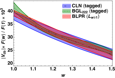
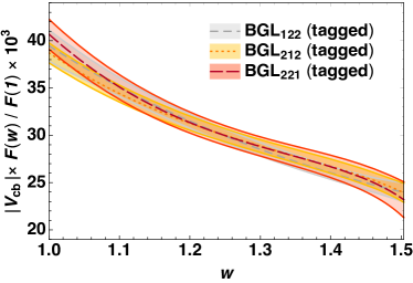
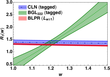
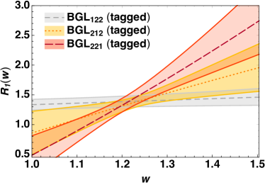
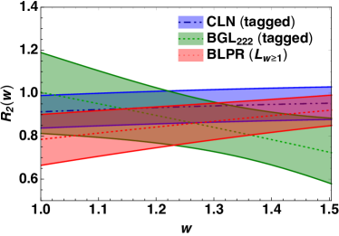
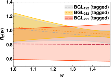
The top row in Fig. 1 shows ${\cal F}(w)$ normalized to the lattice QCD value of ${\cal F}(1)$, as $|V_{cb}|\,{\cal F}(w)/{\cal F}(1)$ for six fits. The left-side plots show three previously published fits: the ${\rm BGL}_{{2}{2}{2}}$ and CLN fit results, based on the 2017 Belle tagged measurement, and the ‘BLPR’ result of Ref. Bernlochner et al. (2017b), which performed an HQET-based fit to both $B\to D^{*}l\bar{\nu}$ and $B\to Dl\bar{\nu}$ data to determine the subleading ${\cal O}(\Lambda_{\rm QCD}/m_{c,b})$ Isgur-Wise functions, using also lattice QCD information. The right-side plots in Fig. 1 show the ${\rm BGL}_{{1}{2}{2}}$, ${\rm BGL}_{{2}{1}{2}}$, and ${\rm BGL}_{{2}{2}{1}}$ fits, based on the 2017 Belle tagged measurement Abdesselam et al. (2017). The shaded bands indicate the uncertainties. The ${\rm BGL}_{{2}{2}{2}}$ and ${\rm BGL}_{{2}{2}{1}}$ fits have the largest differential rates near zero recoil ($w=1$), corresponding to the largest extracted values of $|V_{cb}|$.

The value of $|V_{cb}|$ extracted from the ${\rm BGL}_{{1}{2}{2}}$ fit to the 2017 Belle unfolded measurement Abdesselam et al. (2017) is more than $1\sigma$ smaller than in the 6-parameter ${\rm BGL}_{{2}{2}{2}}$ fit to the same data. This raises several questions: Would a ${\rm BGL}_{{2}{2}{2}}$ fit to the 2018 Belle measurement Abdesselam et al. (2018) find a larger value of $|V_{cb}|$ than that in Eq. (2b), closer to its inclusive determination? The consistency of the fitted ${\rm BGL}_{{1}{2}{2}}$ coefficients from the 2017 and 2018 Belle measurements is only at about the $2\sigma$ level for $\tilde{a}_{0}$.

Also shown in Fig. 1 are the fit results for the form factor ratios $R_{1,2}(w)$. The ${\rm BGL}_{{2}{2}{2}}$ fit to the tagged Belle measurement Abdesselam et al. (2017) indicated a substantial deviation from heavy quark symmetry, in particular for the $R_{1}$ form factor ratio Bernlochner et al. (2017a). The central values, for fixed quark mass parameters, at order ${\cal O}(\Lambda_{\rm QCD}/m_{c,b},\,\alpha_{s})$ are Bernlochner et al. (2017a),

$$R_{1}(1) =1.34-0.12\eta(1)+\ldots\,,$$

$$R^{\prime}_{1}(1) =-0.15+0.06\,\eta(1)-0.12\,\eta^{\prime}(1)+\ldots\,,$$ (10)

where $\eta(w)$ is a ratio of a subleading and the leading Isgur-Wise function. With $\eta(1)$ and $\eta^{\prime}(1)$ of order unity, $R_{1}(1)$ cannot be much below 1, and $|R^{\prime}_{1}(1)|$ cannot be large, without a breakdown of heavy quark symmetry. Preliminary lattice QCD calculations Aviles-Casco et al. (2018); Kaneko et al. (2018) also do not indicate ${\cal O}(1)$ violations of heavy quark symmetry. Figure 1 shows that the ${\rm BGL}_{{1}{2}{2}}$ fit exhibits better agreement with heavy quark symmetry expectations for $R_{1}(w)$. However, this likely arises because $R_{1}(w)\propto(w+1)\,g/f$, so setting $a_{1}=0$ constrains the shape of the numerator. By contrast, the ${\rm BGL}_{{2}{1}{2}}$, ${\rm BGL}_{{2}{2}{1}}$, and ${\rm BGL}_{{2}{2}{2}}$ fits prefer $a_{1}\neq 0$, and yield $R_{1}(w)$ in some tension with heavy quark symmetry and lattice QCD.

V Toy studies

Figure 2: The pull constructed from a large ensemble of pseudo-experiments using 3rd order terms of the $1\times$ scenario (left plot) and $10\times$ scenario (right plot) described in the text. The pull of the fits selected by the nested hypothesis prescription (black) show no bias or under-coverage of uncertainties. Also shown in red is the pull from a ${\rm BGL}_{{1}{2}{2}}$ fit, showing a large bias on the value of $|V_{cb}|$. Mean ($\mu$) and standard deviation ($\sigma$) from normal distributions fitted to the ensembles are also provided.

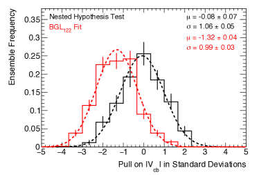
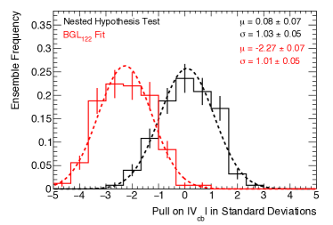
To validate the prescription outlined above, and to demonstrate that it yields an unbiased value of $|V_{cb}|$, we carried out a toy MC study using ensembles of pseudo-data sets. These were generated using the ${\rm BGL}_{{3}{3}{3}}$ parametrization, i.e., with nine coefficients. The six lower order coefficients $\{\tilde{a}_{0,1},\,\tilde{b}_{0,1},\,\tilde{c}_{1,2}\}$ were chosen to be identical to the ${\rm BGL}_{{2}{2}{2}}$ fit results of Fig. 1. The 3rd order terms $\{\tilde{a}_{2},\,\tilde{b}_{2},\,\tilde{c}_{3}\}$ were chosen according to two different scenarios: either 1 or 10 times the size of the $\{\tilde{a}_{1},\,\tilde{b}_{1},\,\tilde{c}_{2}\}$ coefficients in the ${\rm BGL}_{{2}{2}{2}}$ fit, as shown in Table 4. We call these the “$1\times$” and “$10\times$” scenarios, respectively. Ensembles were constructed as follows. First, predictions for the 40 bins of the tagged measurement Abdesselam et al. (2017) were produced. Ensembles of pseudo-data sets were then generated using the full experimental covariance, assuming Gaussian errors, and then each pseudo-data set was fit according to the nested hypothesis test prescription.

Parameter	$1\times$ scenario	$10\times$ scenario
$\tilde{a}_{2}\times 10^{2}$	$2.6954$	$26.954$
$\tilde{b}_{2}\times 10^{2}$	$-0.2040$	$-2.040$
$\tilde{c}_{3}\times 10^{2}$	$0.5350$	$5.350$

Table 4: Fit coefficients used to construct the ensembles of toy experiments. The third order terms $\{\tilde{a}_{2},\tilde{b}_{2},\tilde{c}_{3}\}$ are taken either as 1 or 10 times the second order terms $\{\tilde{a}_{1},\tilde{b}_{1},\tilde{c}_{2}\}$ in the ${\rm BGL}_{{2}{2}{2}}$ fit shown in Fig. 3.

	${\rm BGL}_{{1}{2}{2}}$	${\rm BGL}_{{2}{1}{2}}$	${\rm BGL}_{{2}{2}{1}}$	${\rm BGL}_{{2}{2}{2}}$	${\rm BGL}_{{2}{2}{3}}$	${\rm BGL}_{{2}{3}{2}}$	${\rm BGL}_{{3}{2}{2}}$	${\rm BGL}_{{2}{3}{3}}$	${\rm BGL}_{{3}{2}{3}}$	${\rm BGL}_{{3}{3}{2}}$	${\rm BGL}_{{3}{3}{3}}$
$1\times$ scenario	6%	0%	37%	27%	6%	6%	11%	0%	2%	4%	0.4%
$10\times$ scenario	0%	0%	8%	38%	14%	8%	16%	3%	4%	8%	1%

Table 5: The frequency of the selected hypotheses for ensembles created with the two scenarios for the higher order terms, as estimated with an ensemble size of 250 pseudo-data sets.

The frequency with which particular ${\rm BGL}_{{i}{j}{k}}$ parametrizations are selected are shown in Table 5, for both the $1\times$ and $10\times$ scenarios. For each selected fit hypothesis, the recovered value, $|V_{cb}|_{\text{rec}}$, and the associated uncertainty, $\sigma$, may then be used to construct a pull, i.e., the normalized difference $(|V_{cb}|_{\text{rec}}-|V_{cb}|_{\text{true}})/\sigma$, where $|V_{cb}|_{\text{true}}$ is the ‘true’ value used to construct the ensembles. If a fit or a procedure is unbiased, the corresponding pull distribution should follow a standard normal distribution (mean of zero, standard deviation of unity). In Fig. 2 the pull distributions for both the $1\times$ and $10\times$ scenarios are shown and compared to that of the ${\rm BGL}_{{1}{2}{2}}$ parametrization. One sees that the nested hypothesis test proposed in this paper selects fit hypotheses that provide unbiased values for $|V_{cb}|$ in both scenarios. However, the ${\rm BGL}_{{1}{2}{2}}$ fit shows significant biases. In the ensemble tests the ${\rm BGL}_{{1}{2}{2}}$ fits have mean $\chi^{2}$ values of 41.0 and 56.6, respectively (with 35 degrees of freedom). For the $1\times$ scenario, this produces an acceptable fit probability on average. Nonetheless, the recovered value of $|V_{cb}|$ is biased by about $1.3\,\sigma$.

VI conclusions

We studied the differences of the determinations of $|V_{cb}|$ from exclusive semileptonic $B\to D^{*}\ell\nu$ decays, depending on the truncation order of the BGL parametrization of the form factors used to fit the measured differential decay distributions. Since the 2018 untagged Belle measurement Abdesselam et al. (2018) used a five-parameter BGL fit, Refs. Grinstein and Kobach (2017); Bernlochner et al. (2017a) used a six-parameter fit, and Refs. Bigi et al. (2017a); Jaiswal et al. (2017) used an eight-parameter one, we explored differences between the five, six, seven, and eight parameter fits.

We proposed using nested hypothesis tests to determine the optimal number of fit parameters. For the 2017 Belle analysis Abdesselam et al. (2017), six parameters are preferred. Including additional fit parameters only improves $\chi^{2}$ marginally. Comparing the result of the ${\rm BGL}_{{1}{2}{2}}$ fit used in the 2018 untagged Belle analysis Abdesselam et al. (2018) to the corresponding fit to the 2017 tagged Belle measurement Abdesselam et al. (2017), up to $2\sigma$ differences occur, including in the values of $|V_{cb}|$. This indicates that more precise measurements are needed to resolve tensions between various $|V_{cb}|$ determinations, and that the truncation order of the BGL expansion of the form factors has to be chosen with care, based on data.

We look forward to more precise experimental measurements, more complete fit studies inside the experimental analysis frameworks, as well as better understanding of the composition of the inclusive semileptonic rate as a sum of exclusive channels Bernlochner et al. (2012, 2014). Improved lattice QCD results, including finalizing the form factor calculations in the full $w$ range Aviles-Casco et al. (2018); Kaneko et al. (2018) are also expected to be forthcoming. These should all contribute to a better understanding of the determinations of $|V_{cb}|$ from exclusive and inclusive semileptonic decays, which is important for CKM fits, new physics sensitivity, $\epsilon_{K}$, and rare decays.