Strong deformation of ferrofluid-filled elastic alginate capsules in inhomogenous magnetic fields

Abstract

We present a new system based on alginate gels for the encapsulation of a ferrofluid drop, which allows us to create millimeter-sized elastic capsules that are highly deformable by inhomogeneous magnetic fields. We use a combination of experimental and theoretical work in order to characterize and quantify the deformation behavior of these ferrofluid-filled capsules. We introduce a novel method for the direct encapsulation of unpolar liquids by sodium alginate. By adding 1-hexanol to the unpolar liquid, we can dissolve sufficient amounts of $\mathrm{CaCl_{2}}$ in the resulting mixture for ionotropic gelation of sodium alginate. The addition of polar alcohol molecules allows us to encapsulate a ferrofluid as a single phase rather than an emulsion without impairing ferrofluid stability. This encapsulation method increases the amount of encapsulated magnetic nanoparticles resulting in high deformations of approximately 30% (in height-to-width ratio) in inhomogeneous magnetic field with magnetic field variations of $50\,\mathrm{mT}$ over the size of the capsule. This offers possible applications of capsules as actuators, switches, or valves in confined spaces like microfluidic devices. We determine both elastic moduli of the capsule shell, Young’s modulus and Poisson’s ratio, by employing two independent mechanical methods, spinning capsule measurements and capsule compression between parallel plates. We then show that the observed magnetic deformation can be fully understood from magnetic forces exerted by the ferrofluid on the capsule shell if the magnetic field distribution and magnetization properties of the ferrofluid are known. We perform a detailed analysis of the magnetic deformation by employing a theoretical model based on nonlinear elasticity theory. Using an iterative solution scheme that couples a finite element / boundary element method for the magnetic field calculation to the solution of the elastic shape equations, we achieve quantitative agreement between theory and experiment for deformed capsule shapes using the Young modulus from mechanical characterization and the surface Poisson ratio as a fit parameter. This detailed analysis confirms the results from mechanical characterization that the surface Poisson ratio of the alginate shell is close to unity, that is, deformations of the alginate shell are almost area conserving.

I Introduction

Ferrofluids contain dispersed magnetizable nanoparticles, which are long-time stable and exhibit superparamagnetic behavior Rosenweig (1985). Ferrofluids can be actuated by magnetic fields and have various technical and medical applications Voltairas et al. (2001); Holligan et al. (2003); Liu et al. (2007). In many applications it is of interest to prevent a ferrofluid from interaction with its environment, especially considering its corrosive effects on metals. This can be achieved by encapsulation of a ferrofluid drop with a thin protective shell made, for example, from a gel or soft elastic material. The result is an elastic capsule with a stable ferrofluid droplet inside. The elastic shell protects the inner fluid from direct interaction with the environment but it can be deformed by various external forces Fery et al. (2004); Fery and Weinkamer (2007). Elastic capsules are stable under uniform pressure up to a buckling threshold Zoldesi et al. (2008); Gao et al. (2001); Knoche and Kierfeld (2011). Buckling indentations can also be induced by point forces Fery et al. (2004); Vella et al. (2012) and capsules can be deformed in hydrodynamic flow Barthès-Biesel (2011). Other deformation techniques include compression between parallel plates Carin et al. (2003); Fery and Weinkamer (2007) or in a spinning drop apparatus Pieper et al. (1998), or pendant capsule elastometry Knoche et al. (2013); Hegemann et al. (2018). These mechanical deformation techniques can be employed to determine the elastic moduli of capsule shells. Whereas these deformation techniques require direct mechanical interaction with the capsules, deformation can also be driven by external electric or magnetic fields if the capsules are filled by a dielectric liquid or ferrofluid Degen et al. (2008a); Karyappa et al. (2014); Wischnewski and Kierfeld (2018) or if the shell itself contains magnetizable particles Loukaides et al. (2014); Seffen and Vidoli (2016). In particular, we demonstrate in this paper that magnetic actuation and mechanical characterization of a capsule filled with a ferrofluid is possible by deformation in a magnetic field.

The aim of this work is the encapsulation of a stable ferrofluid drop with high magnetic nanoparticle concentration in order to achieve strong deformation in an external magnetic field and a quantitative understanding of the deformation behavior by comparison to theoretical predictions based on nonlinear elasticity theory. Encapsulation of stable ferrofluids was achieved in Refs. 21; 22, for example, for magnetic resonance imaging Shen et al. (2003). Ferrofluid concentration inside the capsules were low, however, such that there are no reports on actuation and deformation properties in magnetic fields. On the other hand, magnetic deformation of capsules filled with magnetic particles was reported in Refs. 23; 24; these magnetic particles, however, aggregated and did not remain in a stable ferrofluid state. The aim of this work is a reliable capsule system, into which a stable ferrofluid can be loaded at high concentration such that it can strongly deform in magnetic fields, which is important for possible applications of capsules as actuators, switches, or valves.

We present a new method to achieve stable ferrofluid encapsulation at high concentrations. Generally, encapsulation of magnetic nanoparticles in a stable dispersion in the liquid core is a difficult task. Here we use alginate gel as shell material. Because of its mild gelation conditions, non-toxicity and biocompatibility, it is a widely used encapsulation material Martins et al. (2015); Degen et al. (2015); Martins et al. (2017); Lee and Mooney (2012); Leong et al. (2016); Prakash (2007) Sodium alginate is soluble in water, and ionotropic gelation takes place upon contact with bi- or trivalent cations Ouwerx et al. (1998); Mørch et al. (2006); usually, calcium is used for the gelation. Magnetic nanoparticles, which are sterically stabilized by amphiphiles such as lauric acid or electrostatically stabilized, destabilize and flocculate in the presence of calcium ions if both ions and nanoparticles are in the aqueous phase in the liquid core of the capsule Degen et al. (2015). To reduce this effect oil-soluble magnetic particles can be used, which are encapsulated in an oil in water emulsion, where calcium is solved in the aqueous emulsion phase Martins et al. (2017). In previous work, we showed that encapsulation of a stable ferrofluid is possible with this technique and that a significant deformation in magnetic fields can be achieved Zwar et al. (2018). The deformation was, however, limited to approximately 10% because magnetic nanoparticles are only contained in the oil emulsion phase, whereas a certain amount of unmagnetizable aqueous emulsion phase is needed to solve calcium ions. In order to further increase the magnetic nanoparticle content in the liquid core of the capsule we use 1-hexanol as a solvent with high polarity but low water-solubility to dissolve significant amounts of calcium chloride. We mix 1-hexanol with chloroform as a second solvent because the magnetite nanoparticles are not dispersable in pure 1-hexanol. Chloroform also increases the density of the liquid core which improves experimental handling of the capsules. The general principle of using 1-hexanol as an additive can be extended to a variety of oils. The advantage of direct oil encapsulation concerning the encapsulation of ferrofluids is the higher magnetic content, which leads to higher deformation in the same magnetic field. In emulsion-based systems the need for a second phase reduces the overall nanoparticle concentration and thus the reaction to magnetic fields.

The ferrofluid-filled capsule represents a magnetic dipole. In order to achieve strong deformation we use inhomogeneous magnetic fields, which are easily realizable and result in a net force onto the ferrofluid-filled capsule. We use this net force to deform the capsule by pushing the flexible particle against the bottom wall of the cuvette. In principle, deformation and shape transitions are also possible in homogeneous magnetic fields, which tend to stretch the capsule in order to increase the dipole moment Wischnewski and Kierfeld (2018). For a quantitative understanding of the deformation behavior we measure the magnetic field distribution, calculate the magnetic properties of the ferrofluid from the nanoparticle size distribution and compare the experimental capsule shapes to theoretical shapes calculated using nonlinear elasticity theory by a coupled finite element method (FEM) for the elastic problem and a boundary element method (BEM) for the magnetic field calculation. This enables us to also obtain additional information not easily accessible in experiments such as a detailed picture of the magnetic field distribution and the elastic stress distribution in the capsule, which are important, for example, to predict capsule rupture because of magnetic deformation.

II Materials and methods

II.1 Preparation of the magnetic nanoparticles

The magnetite nanoparticles ($\mathrm{Fe_{3}O_{4}}$) used in this work were synthesized following a procedure by Sun et al. Sun et al. (2004). These particles are crystalline, and usually show a narrow size distribution around an average of 6 nm diameter. The small size is important for the stability of the resulting ferrofluid. Additional stabilization is provided by the surfactants oleic acid and oleyl amine which hinder agglomeration.

II.2 Preparation of capsules

We encapsulate a mixture of chloroform and 1-hexanol (7:3) containing dispersed magnetite nanoparticles with a mass concentration $c_{m}=516\,\mathrm{g}/\mathrm{mol}$ in an alginate gel shell. Initially, calcium chloride is dissolved in the 1-hexanol/chloroform mixture (by volume 3:7) in order to perform the alginate gelation. Two additional surfactants stabilizing the nanoparticles, oleic acid and oleylamine, also accelerate the gelation and are added with 1%_V (volume percent) each to improve the process.

The high chloroform content requires to adjust the capsule preparation process, which is normally done by dripping one component, either sodium alginate or calcium chloride solution, directly (from air) into the other liquid. Because of the high chloroform content of 70%_V, dripping of the 1-hexanol/chloroform mixture containing the calcium chloride from air into the alginate solution is not feasible because the mixture spreads on the interface. Instead we first overlay a cylinder which is filled to 7/8 with sodium alginate solution (1% by weight) with distilled water and form a droplet of the 1-hexanol/chloroform mixture in the water layer using a capillary, see Figure 1). The droplet then falls through the interface between water and alginate solution without spreading. Within the alginate solution, the calcium chloride dissolved in the 1-hexanol/chloroform droplet starts the gelation. In order to avoid contact with the glass surface a seal (shown in grey in Figure 1) can be placed over the opening and the cylinder can be turned for 30 s.

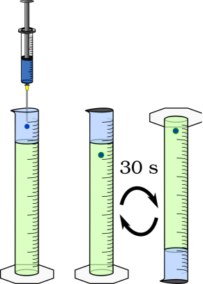
Figure 1: Procedure for the production of ferrofluid-filled capsules, dark blue = 1-hexanol/chloroform mixture containing calcium chloride and magnetic nanoparticles, light blue = water, green = sodium alginate solution

The capsules are washed with water to stop the polymerisation and placed in saturated sodium alginate solution. This lowers the elastic moduli of alginate systems and thus lead to capsules that are easier to deform Zwar et al. (2018).

II.3 Experimental setup for mechanical characterization

For mechanical characterization of the capsule shells we use two methods, compression between parallel plates and deformation in a spinning drop apparatus. Combination of the results from both measurements will enable us to determine both the two-dimensional Young modulus $Y_{2\text{D}}$ and the surface Poisson ratio $\nu$.

In the compression method a capsule is placed between two parallel plates and the force is measured as a function of the displacement. A sketch of the method is shown in the Supporting Information. Compression between parallel plates was performed with the DCAT11 tensiometer (DataPhysics Instruments GmbH) with the software SCAT. The compression speed was set to $0.02\,\mathrm{mm/s}$.

In a spinning drop apparatus, a capsule is placed in a capillary filled with a liquid of higher density $\rho$ and monitored with a camera (see Supporting Information). During rotation of the capillary, the capsule moves to the horizontal axis of the capillary and deforms. The deformation is measured as a function of angular rotation frequency. For the spinning capsule experiments, we used the SVT 20 of the DataPhysics Instruments GmbH. We used Fluorinert 70 (FC 70) as outer phase because of its high density. The initial undeformed (quiescent) capsule state was recorded at 2000 rpm.

Capsule radii were determined by image analysis of capsule photos (see Supporting Information). For the shell thickness this image analysis could not be used because of the small thickness. Thus, scanning electron microscopy (SEM) measurements were performed to estimate the shell thickness. From the images shown in the Supporting Information, it can also be concluded that the nanoparticles were not incorporated in the shell.

II.4 Experimental setup for magnetic deformation

The ferrofluid filled capsule is placed at the bottom of a nonmagnetic cuvette. This cuvette was placed right above the conical iron core of a coil. This way, the capsule was as close as possible to the tip of the cone (the bottom of the capsule was about 2.6 mm above the iron core) and exceeded a maximum field strength. In Figure 2, the experimental setup for the deformation of capsules in magnetic fields is shown.

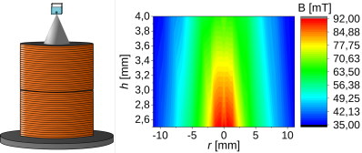
Figure 2: Experimental setup and measured flux density for the magnetic deformation of capsules with a current of $I=2\,$A.

II.5 Elastic and magnetic model for deformation

In order to model the magnetic deformation of a capsule we need an elastic material model for the capsule shell and a magnetic model for the calculation of the magnetic forces. To calculate the shape of a deformed capsule, we use a small strain nonlinear shell theory with a Hookean elastic law Knoche and Kierfeld (2011); Knoche et al. (2013); Knoche and Kierfeld (2014). In our model, we assume a very thin, effectively two-dimensional elastic shell and rotational symmetry. We also assume that the capsule attains a perfectly spherical stress-free reference shape with rest radius $R_{0}$ during the polymerization process. All these assumptions hold to a good approximation in the experimental realization. Once the elastic shell is polymerized, there is no exchange of fluid between the inner phase and the outer phase possible anymore, at least under the employed experimental conditions and during magnetic deformation. So the volume $V_{0}$ of the capsule remains constant. The capsule is then deformed by a hydrostatic pressure caused by the density difference $\Delta\rho$ between the inner phase and the outer phase. In the presence of an additional magnetic field, the magnetic stress caused by the ferrofluid deforms the capsule as well. We consider capsules which sink to the bottom of a cuvette where also the magnetic deformation takes place, and both gravity and magnetic forces press the capsule against the bottom wall of the cuvette. In a steady state without motion, the fluid can only exert normal forces on the surface. The normal forces caused by the ferrofluid are given by Rosenweig (1985)

$$\begin{split}f_{m}(r,z)&=\mu_{0}\int\limits_{0}^{H(r,z)}M(r,z)\text{d}H^{\prime}(r,z)\\ &\quad+\frac{\mu_{0}}{2}M_{n}^{2}(r,z)\end{split}$$ (1)

($M$ and $M_{n}$ are absolute value and normal component of the magnetization ${\bf M}$, $H$ the magnetic field, and we use cylindrical coordinates $r$ and $z$; for a ferrofluid we can safely assume that ${\bf M}$ and ${\bf H}$ are parallel). The deformed shape of the capsule can be calculated by using a system of six nonlinear differential equations, the shape equations, see Ref. 9 for a derivation and the Supporting Information for more details.

There are two material parameters, the two-dimensional Young modulus $Y_{2\text{D}}$ and the surface Poisson ratio $\nu$, that enter the theoretical model. These parameters are obtained from the mechanical characterization of the capsule by plate compression and spinning capsule deformation as explained below in the Experiments and Results section. Moreover, the rest radius $R_{0}$ of the initially spherical capsule and the thickness $h$ of the shell are needed. The thickness $h$ determines the bending modulus via $E_{B}=Y_{2\text{D}}h^{2}/12(1-\nu^{2})$ and $R_{0}$ the initial rest shape with respect to which elastic strains and stresses are obtained and the fixed volume $V_{0}$. Moreover, the density difference $\Delta\rho$ between the interior and exterior liquid phases is needed for the hydrostatic pressure.

In addition, the effective interface tension $\gamma$ between the inner liquid phase and the elastic shell and between the shell and the outer liquid phase has to be estimated, but is very difficult to be measured. Generally we expect solid-liquid surface tensions to be smaller than liquid-liquid surface tensions Mondal et al. (2015). Because the shell can still contain pores leading to liquid-liquid contact, we expect the interface tension $\gamma$ to be lower than but similar to the interfacial tension between outer and inner liquid. The interfacial tension of a similar system without elastic shell and without nanoparticles inside was determined to be $14.6\,\text{mN}/\text{m}$ by pendant drop tensiometry. The presence of surfactants from the synthesis of the nanoparticles as well as the elastic shell should lower the interface tension below this value. In addition, it should be mentioned that the interfacial tension of the ferrofluid is probably increasing for increasing external magnetic field as Afkhami et al. observed Afkhami et al. (2010). We expect $\gamma\approx 10\pm 4\,\text{mN}/\text{m}$ to be a valid average value.

The parameter values that are used for the numerical calculation of capsule shapes are summarized in Table 1. The surface Poisson ratio deviates slightly from the value measured in the experiment (eq 11). This will be discussed below in the Results section.

Name	Symbol	Value
2D Young’s modulus	$Y_{2\text{D}}$	$0.186\,\text{N}/\text{m}$
Surface Poisson ratio	$\nu$	0.946
Shell thickness	$h$	$3\,\mu\text{m}$
Radius	$R_{0}$	$0.903$ …
		$1.044\,\text{mm}$
Density difference	$\Delta\rho$	$0.24\,\text{g}/\text{cm}^{3}$
Surface tension	$\gamma$	$10\,\text{mN}/\text{m}$

Table 1: Numerical parameters

Finally, the exact distribution of the applied inhomogeneous magnetic field and the magnetic properties of the ferrofluid, that is, its magnetization curve $M=M(H)$ have to be known as well in order to calculate the magnetic forces (eq 1), see following sections.

II.6 Magnetic field

We used a Hall probe to measure the magnetic field depending on the position and the applied current $I$ in the coil (see Figure 2). The capsules are very small in relation to the size of the coil and the conical iron core, so the radial component of the magnetic field can be neglected. In addition, the $z$-component of the field is nearly constant in radial direction over the capsule size and thus only depends on the $z$-coordinate. In the numerical calculations we use a fit to the measured external magnetic field with a Langevin function to model the dependence on current $I$ and a hyperbolic function for the dependence on height $z$,

$$B_{z}(z,I)=a\left(\coth(b_{I}I)-\frac{1}{b_{I}I}\right)\left(\frac{a_{z}}{z-b_{z}}+c_{z}\right).$$ (2)

with fit parameters $a=4.647$, $b_{I}=0.332\,\mathrm{A^{-1}}$, $a_{z}=286.7\cdot 10^{-6}\,\mathrm{Tm}$, $b_{z}=-1.104\cdot 10^{-3}\,\mathrm{m}$, and $c_{z}=10.86\cdot 10^{-3}\,\mathrm{T}$. A plot of the fit curve together with the measured magnetic field is shown in the Supporting Information. The fit describes the magnetic field with an error below 1 % in the neighborhood of the capsule.

II.7 Magnetization curve

The magnetization curve of the ferrofluid is calculated from the particle size distribution of the magnetite nanoparticles. The particle size distribution is obtained from dynamic light scattering (see Supporting Information) and given in Table 2, where the relative frequency $n_{i}$ of particle diameters $d_{i}=5-14\,\mathrm{nm}$ are given. The particle size distribution has a maximum around $d=7-8\,\mathrm{nm}$.

$d_{i}$ [nm]	$n_{i}$ [%]	$d_{i}$ [nm]	$n_{i}$ [%]
5	2.0	10	8.6
6	14.1	11	7.6
7	23.9	12	5.5
8	23.9	13	3.8
9	16.1	14	2.4

Table 2: Particle size distribution: relative frequency $n_{i}$ of particle diameter $d_{i}$.

According to Ref. 1 the magnetization $M$ as a function of the field strength $H$ is then given by

$$\begin{split}M(H)&=M_{s}\sum\limits_{i}n_{i}(d_{i}-d_{s})^{3}\times\\ &L\left[\frac{\mu_{0}M_{d}H}{k_{b}T}\frac{\pi}{6}(d_{i}-d_{s})^{3}\right]\bigg{/}\sum\limits_{i}n_{i}d_{i}^{3}\end{split}$$ (3)

with the Langevin function $L(x)=\coth(x)-1/x$. $M_{s}=34650\,{\text{A}}{\text{m}^{-1}}$ is the saturation magnetization of the magnetite particles without sterical stabilization and $M_{d}=446000\,{\text{A}}{\text{m}^{-1}}$ denotes the bulk magnetization of magnetite. The diameters of the nanoparticles are reduced by $d_{s}$, because the crystal order of the outer surface layer of magnetite is disturbed by the dispersing agent. This lowers also the effective saturation magnetization of the ferrofluid. Following Ref. 1 we use $d_{s}=1.66\,\text{nm}$. The resulting magnetization curve is shown in Figure 3.

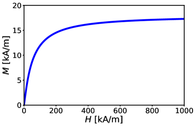
Figure 3: Magnetization curve of the ferrofluid used in the experiment according to eq 3.

II.8 Numerical procedure

The calculation of the magnetic field inside the capsule and the ferrofluid is done numerically by a coupled FEM/BEM Costabel (1987); Wendland (1988); Arnold and Wendland (1983, 1985); Ligget and Salmon (1981); Lavrova et al. (2005, 2006); Harris and Basaran (1993). The shape of the elastic shell and the magnetic field inside the capsule form a coupled problem that has to be solved self-consistently: Changes in the shape of the elastic shell cause changes in the magnetic field distribution inside the capsule, which, in turn, changes the magnetic forces in eq 1 onto the capsule shell and thus the capsule shape. Therefore, an iterative solution scheme has to be used. For a given trial shape, we calculate the magnetic field inside the capsule using only the externally applied field. Using the new field, we can recalculate the magnetic forces and a new equilibrium shape. This is iterated until shape and field converge to a fixed point. This iterative solution scheme for a ferrofluid-filled capsule has been introduced and is explained in detail in Ref. 18.

III Experiments and Results

III.1 Mechanical characterization of the capsule shell

We first characterize the capsules mechanically and determine the two-dimensional Young modulus $Y_{2\text{D}}$ and the surface Poisson ratio $\nu$. These values are subsequently used in the theoretical model for magnetic deformation. We determine mechanical parameters of the shell with two independent methods, compression between parallel plates and spinning capsule deformation. If the Poisson’s ratio $\nu$ is known both methods give the two-dimensional elastic modulus $Y_{2\text{D}}$. A separate measurement of $\nu$ is, however, difficult and often a generic value is assumed Ben Messaoud et al. (2016); Leick et al. (2010). By combining the results of the two independent measurements, we overcome this problem and obtain two independent equations for the two unknowns $Y_{2\text{D}}$ and $\nu$, which enables us to determine both quantities Leick et al. (2011).

The first method, the compression between parallel plates (capsule squeezing) is a well-known technique for the mechanical characterization of capsules Carin et al. (2003); Fery and Weinkamer (2007). A capsule is placed between two parallel plates and the force is measured as a function of the displacement. From the force-displacement compression curve, elastic moduli of the capsule shell can be calculated. There are different methods to analyze the force-displacement curves. Some methods, like the one developed by Barthès-Biesel et al., use a fit of the whole curve Carin et al. (2003); Fery and Weinkamer (2007). As shown in an earlier publication water leaks out of alginate capsules during compression Degen et al. (2015). Therefore, we only analyze the linear regime with low forces in order to minimize the influence of water leakage.

To describe the compression of a capsule between parallel plates in the initial linear regime, the model of Reissner for a point force acting on the apex of the capsule can be used Fery and Weinkamer (2007); Reissner (1946a, b). In this model the force $F$ depends linearly on the displacement $d$ as

$$F=\frac{4Y_{2\text{D}}h}{R_{0}\sqrt{3(1-\nu^{2})}}\>d.$$ (4)

Reissner’s linear theory applies to an unpressurized shell with purely elastic tensions and rest radius $R_{0}$. Here, we need to generalize this model to include the interfacial tension $\gamma$, which generates a stretching tension in the shell already before indentation by the force. We find that the effect of an additional interfacial tension $\gamma$ is equivalent to the effect of an internal pressure $p_{0}=2\gamma/R_{0}$ given by the Laplace-Young equation; such pressurized capsules have been studied previously by Vella et al. in Ref. 10. Using this equivalence we obtain a modified linear force-displacement relation

$$F=\frac{4Y_{2\text{D}}h}{R_{0}\sqrt{3(1-\nu^{2})}}\>G(\tau)\>d$$ (5)

with

$$G(\tau) =\frac{\pi}{2}\frac{(\tau^{2}-1)^{1/2}}{\operatorname{artanh}{(1-\tau^{-2})^{1/2}}}$$ (6)

$$\tau =3(1-\nu^{2})\left(\gamma/Y_{2\mathrm{D}}\right)^{2}\left(R_{0}/h\right)^{2}$$

(more details on the derivation are given in the Supporting Information). Note that a vanishing interface tension ($\gamma=0$) leads to $G(0)=1$, and we recover the Reissner result (eq 4). To obtain the elastic moduli from this linear model, also the radius of the undeformed capsule $R_{0}$ and the thickness of the shell $h$ are needed.

The second method for the determination of $Y_{2\text{D}}$ and $\nu$ is the spinning capsule method. Originally, the spinning drop method was developed for interfacial tension measurements Vonnegut (1942); Princen et al. (1967). A drop is placed in a capillary filled with a liquid of higher density $\rho$. During rotation of the capillary the drop deforms; the shape of the deformed drop depends on the rotation frequency and interfacial tension $\gamma$. For the deformation of liquid-filled capsules, Pieper et al. developed a model that allows one to obtain in an analogous fashion 2D elastic moduli from the capsule deformation Pieper et al. (1998). A sketch of the method is shown in the Supporting Information. Initially (at small rotation speed), the capsule is in an undeformed (quiescent) state. Then capsule deformation is measured as a function of the angular rotation frequency $\omega$. The capsule deformation is quantified by the Taylor deformation $D$,

$$D=\frac{l-b}{l+b},$$ (7)

which is determined from the length $l$ and the width $b$ of the capsule. For deformations within the linearly elastic regime, the Taylor deformation depends on the angular rotation frequency $\omega$ via Pieper et al. (1998)

$$D=-\Delta\rho\omega^{2}R_{0}^{3}\frac{(5+\nu)}{16Y_{2\text{D}}},$$ (8)

where $R_{0}$ is the radius of the undeformed capsule, $\Delta\rho$ is the density difference between the inside and outside liquid phases. Equation 8 is only valid for shells with purely elastic tensions and without an interfacial tension. Again we need to generalize the theory to include an interfacial tension $\gamma$. This can be done by observing that the linear response of the capsule deformation in spinning drop experiments is actually equivalent to the linear deformation response of a ferrofluid-filled capsule in a uniform external magnetic field Wischnewski and Kierfeld (2018) with a magnetic susceptibility $\chi=-1$ and a magnetic field strength $\mu_{0}H^{2}=\Delta\rho R_{0}^{2}\omega^{2}$. This equivalence arises because both centrifugal forces exerted by the interior liquid in the spinning capsule geometry and magnetic forces exerted by the ferrofluid in an external field are normal surface forces. Moreover, for a spherical shape they have the same position-dependence for $\chi=-1$ and the same magnitude if we set $\mu_{0}H^{2}=\Delta\rho R_{0}^{2}\omega^{2}$. In Ref. 18 the deformation of a ferrofluid-filled magnetic capsule has already been considered also in the presence of an interfacial tension $\gamma$, and we can exploit the equivalence of both problems and adapt the results of Ref. 18 for the linear response (more details are given in the Supporting Information). We find

$$D=-\Delta\rho\omega^{2}R_{0}^{3}\frac{(5+\nu)}{16[Y_{2\text{D}}+(5+\nu)\gamma]},$$ (9)

that is, in the presence of an interfacial tension we simply have to replace $Y_{2\text{D}}$ in eq 8 by $Y_{2\text{D}}+(5+\nu)\gamma$.

The two unknown material parameters Young’s modulus $Y_{2\text{D}}$ and surface Poisson ratio $\nu$ can now be obtained from solving the two eqs 5 and 9 simultaneously, which can only be done numerically for $\gamma\neq 0$ in general. In order to do so, also the rest radius $R_{0}$ and the shell thickness $h$ of the spherical capsules are needed. The mean capsule radius was determined from image analysis (see Materials and Methods) as 794 $\pm$ 87$\,\mathrm{\mu m}$. The shell thickness was determined by SEM (see Materials and Methods and Supporting Information). The shell thickness estimated by SEM was under $1{\rm\mu mu}$. As SEM is performed in ultra-high vacuum, swelling has to be taken into account. Because we were not able to resolve the hydrated capsule shell by optical microscopy, its thickness has to be below $5\,\mathrm{\mu m}$. We conclude that the shell thickness of hydrated capsules is approximately $3\,\mathrm{\mu m}$ but with a relatively high error around $1\,\mathrm{\mu m}$.

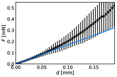
Figure 4: Averaged force($F$)-displacement($d$) curve for capsule compression between parallel plates and fit to the linear regime.

Figure 4 shows the results for the force-displacement curves in the capsule compression tests. We measured 15 individual capsules, and the respective force values for the displacement were averaged to gain information on replicability. In Figure 4 the averaged force-displacement curve is shown. The linear regime can be seen clearly. In this regime the error bars are also relatively low. Higher error bars with increasing compression are an effect of capsule size variations. For the calculation of the elastic moduli, the analysis was performed for each capsule separately with the respective radii and an average value $FR_{0}/d$ is extracted from the linear regime (blue curve in Figure 4).

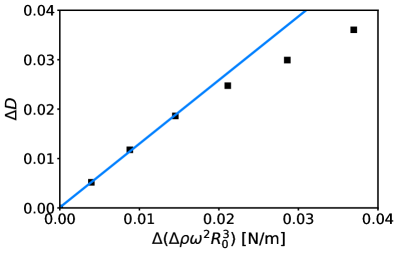
Figure 5: Results of an exemplary spinning capsule experiment for the difference in Taylor deformation $\Delta D$ (see eq 7) between deformed and initial state as a function of $\Delta(\Delta\rho\omega^{2}R_{0}^{3})$.

Figure 5 shows the results of the spinning capsule experiments for one exemplary capsule. Because of small mechanical forces which act during the capsule synthesis, we observed small initial Taylor deformation values of $D_{i}=1-2\%$, which were not caused by deformation in the centrifugal field. Also the initial quiescent capsule state is measured at $\omega_{i}>0$. Therefore, we subtract the initial deformation and initial angular frequency and use the Taylor deformation difference $\Delta D=D-D_{i}$ and the difference $\Delta\omega=\omega-\omega_{i}$ for the analysis. Figure 5 shows the expected linear dependence of $\Delta D$ from the parameter $\Delta(\Delta\rho\omega^{2}R_{0}^{3})$ according to eq 9. The deviations at higher rotation frequencies are caused by water leakage from the capsule, which was also observed in previous studies Zwar et al. (2018). For the calculation of the elastic moduli, the slope $\Delta D/\Delta(\Delta\rho\omega^{2}R_{0}^{3})$ is determined from the initial linear regime (blue curve in Figure 5).

The results from both capsule deformation methods are used to calculate the surface Poisson ratio $\nu$ and the 2D Young modulus $Y_{2\text{D}}$ by solving eqs 5 and 9 simultaneously. We find

$$Y_{2\text{D}} =0.186\pm 0.040\,\mathrm{N/m}$$ (10)

and

$$1-\nu =(1.9\pm 2.8)\cdot 10^{-7}.$$ (11)

Because $\nu$ is extremely close to unity, the two eqs 5 and 9 can be decoupled with negligible error, which leads to the following simplification: We set $\nu=1$ in eq 9 and calculate $Y_{2\mathrm{D}}$ only from the spinning capsule experiment. This value is then used to calculate $\nu$ via eq 5. This decoupling has the additional benefit that we can determine $Y_{2\mathrm{D}}$ from eq 9 for the spinning capsule experiment effectively independently of the shell thickness $h$, which can only be measured with a relatively high error as explained above.

As compared to other calcium alginate capsules, the moduli are very low Ben Messaoud et al. (2016); Zwar et al. (2018). This is likely an effect of the encapsulated components, that is, the nanoparticles or the specific oils used. In emulsion encapsulation, the moduli were lowered by the addition of nanoparticles Degen et al. (2015). As the main goal was to obtain easily deformable capsules, this was achieved by creating very thin shells. A remarkable result is the high surface Poisson ratio, which points to an area-incompressible shell Pieper et al. (1998). Therefore, we further check this finding by adjusting this parameter in the numerical calculation and analysis of the magnetic deformation of the capsule shape to fit the experimental shapes. For Young’s modulus we use the measured value $Y_{2\text{D}}=0.186\,\text{N}/\text{m}$ in the numerical calculations (see Table 1).

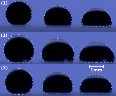
Figure 6: Photographic images of of three different capsules with radii (1) $R_{0}=0.903\,\text{mm}$, (2) $R_{0}=1.044\,\text{mm}$, and (3) $R_{0}=0.965\,\text{mm}$, each for increasing magnetic fields with $I=0\,\text{A}$ (left), $I=2\,\text{A}$ (middle) and $I=5\,\text{A}$ (right). The dashed lines describe numerically calculated capsule contours using the parameters in Table 1. A surface Poisson ratio $\nu=0.946$ gives the best fit to the experimental shapes.

III.2 Magnetic deformation

We prepared different capsules and deformed them with the previously described inhomogenous field by increasing the electric current in the coil up to $5\,\text{A}$. This corresponds to magnetic field variations up to $50\,\mathrm{mT}$ over the size of the capsule. Photos of three exemplary capsules that have reached their steady state of deformation are shown in Figure 6. In Figure 6 we compare these photos with numerically calculated contours (with dashed lines), which were generated with the parameter values in Table 1. These are the experimentally measured parameter values except for the surface Poisson ratio $\nu$. In particular, we consider the mechanical measurements of the Young modulus $Y_{2\text{D}}=0.186\,\mathrm{N/m}$ to be exact and employ this value in the numerics. The Poisson ratio $\nu=1-1.9\cdot 10^{-7}$ from mechanical characterization is extremely close to unity; it depends very sensitively on the shell thickness $h$, which is not easy to determine reliably. Therefore, we regarded $\nu$ as a free parameter and adjusted $\nu$ for the best fit to the experimental shapes, which gives a slightly lower value $\nu\approx 0.946$. This confirms that the surface Poisson ratio of the shell is close to unity.

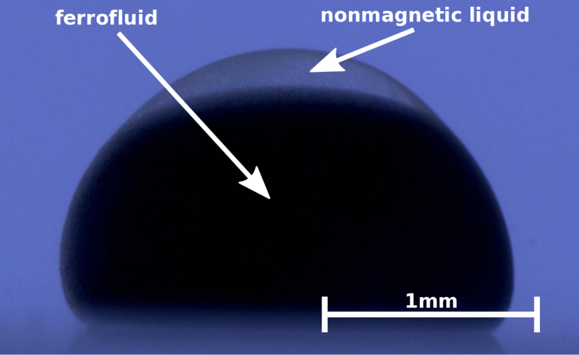
Figure 7: Magnified photographic image of capsule 1 for $I=5\,\text{A}$. A non-magnetic transparent liquid, which is clearly phase-separated from the ferrofluid, is pushed to the upper part of the capsule.

There are minor deviations between experimental capsule shapes and the calculated contours, which are probably caused by inhomogeneities and asymmetries in the shell thickness. In addition, we also observe in Figure 6 that a small amount of transparent non-magnetic liquid was also caught inside the capsules. As the transparent phase spreads lense-like at the surface of the ferrofluid droplet, we assume that this liquid is polar and likely contains water that diffused through the membrane. This liquid is pushed to the upper part of the capsule when the ferrofluid is pushed downwards by the inhomogeneous magnetic field as can be seen in the deformed capsules in Figure 6 and in the close-up in Figure 7. Because this fluid does not contain magnetic nanoparticles, it accumulates at the top of the capsule and, thus, at the place with the lowest field strength during deformation. The appearance of this liquid could not be prevented. The additional error in comparison to the numerical model caused by that liquid should be small, however, because the magnetic stress from the ferrofluid acts on the interface between the ferrofluid and the non-magnetic liquid and is transmitted to the elastic shell by the liquid. Therefore, the behaviour of the whole capsule should be comparable to a capsule with only a ferrofluid inside.

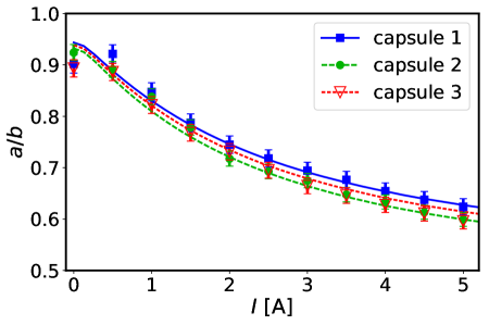
Figure 8: Ratio of capsule height $a$ to width $b$ for increasing current $I$. Markers denote capsules from the experiment, while solid lines represent numerical data generated with the best fit $\nu\approx 0.946$. The upper curve (blue, squares) are data for capsule 1 from Figure 6, the middle curve (red, triangles) and lower curve (green, circles) data for capsules 3 and 2, respectively.

In order to perform a quantitative comparison between numerics and the experiment, we measure the ratio of the capsule’s height ($a$) to the maximum width ($b$), measured parallel to the plate below the capsule. The results of these measurements are shown in Figure 8. We achieve the best agreement between numerical calculations and experimental data for $\nu\approx 0.946$. As also the comparison of capsule shapes in Figure 6 indicates, there is a good agreement between numerical calculations and the experiment for $\nu\approx 0.946$. The only point with some higher deviation is at $I=0$, that is, in the absence of any magnetic field. Then the deformation of the capsule is only caused by gravity and, thus, is in total relatively small. This makes the capsule side ratio $a/b$ very prone to asymmetries of the shell. In addition, the capsule is not a perfect sphere after membrane gelation as it is assumed in the numerical calculation.

We can also check that the capsule’s volume $V_{0}$ remains constant during the magnetic deformation process. Any loss of the inner fluid through the shell would be visually detectable during contact with the outer fluid. In addition, analysis of the capsule photos for the capsule contour $r(z)$ and calculation of the volume $V_{0}=\int dz\pi r^{2}(z)$ does not indicate any loss of volume (see Supporting Information). We conclude that the elastic shell is impermeable for the inner and outer fluid under the employed experimental conditions and during magnetic deformation.

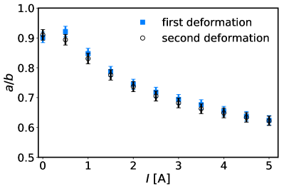
Figure 9: Ratio of the height $a$ of capsule 1 to the width $b$ for increasing current $I$. Squares denote the first deformation. Circles represent a second measurement with the same capsule after deforming and relaxing the capsule.

An important characteristic for possible applications is the question if the material is weakened by the deformation, that is, whether aging effects occur. We checked this by performing a second deformation cycle. The results are shown in Figure 9 exemplarily for the first capsule. Second and first deformation cycles agree well which indicates that no significant damage or aging in the elastic shell occurs during the deformation process. Also the preserved volume during deformation hints at a reversible deformation process.

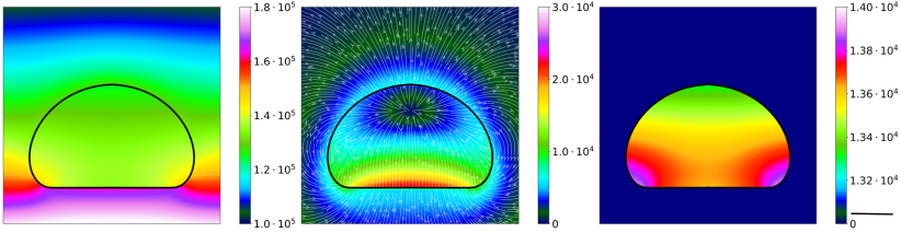
Figure 10: Numerically calculated distributions of magnetic field strength (left), stray field (middle), and magnetization (right) for capsule 1 (see Figure 6) at $I=5$ A. The solid line represents the capsule’s elastic shell. Left: Color codes for the absolute value of the total magnetic field $|\boldsymbol{H}|$ (in A/m). Middle: Color codes for the absolute value of the capsule’s own magnetic stray field $\boldsymbol{H}_{\text{stray}}=\boldsymbol{H}-\boldsymbol{H_{\text{extern}}}$ (in A/m), arrows indicate the field direction. Right: Color codes for the absolute value of the magnetization $|\boldsymbol{M}|$ (in A/m). Note that magnetization variations are very small.

Having established a good agreement between experiment and theory as evidenced by Figures 6 and 8, we can use the theoretical model to access important physical quantities that are experimentally hardly accessible, such as the detailed distributions of magnetic field and stresses. The distribution of the magnetic field inside the deformed capsules is easy to calculate from our model. Figure 10 shows the magnetic field inside and outside of capsule 1 at $I=5$ A, the stray field generated by the magnetized capsule, and the magnetization inside the capsule. The external magnetic field has a high gradient, but the total field inside the capsule is surprisingly homogenous. The magnetization of the ferrofluid decreases the total field in the lower section of the capsule, whereas it increases the total field in the upper part because it counteracts the external magnetic field according to Lenz’s law. This results in smaller field gradients inside the capsule. Magnetization variations inside the capsule are small.

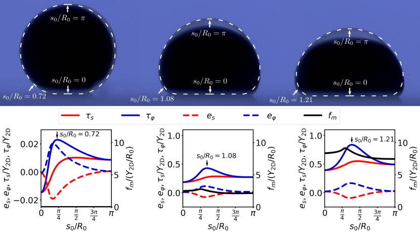
Figure 11: Stresses and strain distributions for different deformation states of capsule 1 (see Figure 6) for zero magnetic field (left), $I=2$ A (middle) and $I=5$ A (right). The left scales show the strain in meridional ($e_{s}$) and circumferential ($e_{\varphi}$) direction and the corresponding elastic stresses ($\tau_{s}$, $\tau_{\varphi}$ in units of $Y_{2\mathrm{D}}$) inside the shell. The right scale shows the magnetic pressure $f_{m}$ (in units of $Y_{2\mathrm{D}}/R_{0}$). The corresponding positions on the surface are given by the arc length $s_{0}$ of the undeformed reference sphere (in units of $R_{0}$, $s_{0}\in[0,\pi]$). For comparison, the interface tension has a value $\gamma=0.054\,Y_{2\mathrm{D}}$. This shows that the interfacial tension $\gamma$ is the dominating stress for small deformations ($e_{s,\varphi}<0.05$) by gravity and at small magnetic field, while the strongly deformed shell is completely dominated by elasticity.

Also the elastic stress state inside the elastic shell as given by the stress and strain distribution becomes accessible by numerical calculation. Figure 11 shows the force/stress/strain distribution along the capsule contour for capsule 1 in different stages of deformation. The position of the highest elastic stress is marked, which is at the highly curved region at the bottom of the capsule. We can infer that the capsule will most likely rupture at this position if the magnetic field is further increased.

III.3 Poisson’s ratio $\nu$

For the numerics, we consider the measurement of the Young-Modulus to be exact with a value of $Y_{2\text{D}}=0.186\,\mathrm{N/m}$. Varying the surface Poisson ratio $\nu$, we find the best match between numerics and experiment for $\nu\approx 0.946$. This confirms a surface Poisson ratio of the shell very close to unity and is only slightly lower than the value $\nu=1-1.9\cdot 10^{-7}$ from mechanical characterization. This represents an explicit measurement of the surface Poisson ratio for an alginate membrane. Other measurements of the surface Poisson ratio of alginate shells are only available for barely comparable systems and solely rely on mechanical characterization Leick et al. (2011); Zwar et al. (2018); in the literature often a generic value (such as $\nu=1/3$ or $\nu\approx 0.5$) is assumed Ben Messaoud et al. (2016); Leick et al. (2010).

The two-dimensional area compression modulus $K_{2\text{D}}=Y_{2\text{D}}/2(1-\nu)$ diverges for $\nu$ close to unity. Therefore, surface Poisson ratios close to unity are remarkable as they imply a polymerized shell that is nearly area preserving during deformation. For Poisson ratios $\nu$ close to unity, strong elastic deformations also become quite sensitive to changes of $\nu$, as the diverging compression modulus also gives rise to diverging elastic stresses containing factors $1/(1-\nu)$. This allows us to determine $\nu$ rather precisely by fitting numerical to experimental shapes (see also Supporting Information).

In a three-dimensional material volume-incompressibility during deformation corresponds to a three-dimensional Poisson ratio $\nu_{3\text{D}}=0.5$ (the three-dimensional compression modulus is $K_{3\text{D}}=Y_{3\text{D}}/3(1-2\nu_{3\text{D}})$). Three-dimensional Poisson ratios close to $\nu_{3\text{D}}=0.5$ are common for three-dimensional polymeric materials, where volume-incompressibility is, for example, explicitly implemented in the Mooney-Rivlin constitutive relation commonly used for polymeric materials Barthès-Biesel et al. (2002). For polymeric materials incompressibility can be attributed to the effectively incompressible densely packed liquid of monomers. Also alginate gels are typically regarded as volume-incompressible materials as confirmed by measurements, for example, in Refs. 53; 54. A material that is volume-incompressible in three dimensions ($\nu_{3\text{D}}=0.5$) forms an area-incompressible thin shell if the shell has constant thickness during deformation. If the thickness can adapt, on the other hand, we expect $\nu=\nu_{3\text{D}}=0.5$ and the thickness grows (shrinks) if the shell area is compressed (expanded). Therefore, our findings are consistent with an alginate shell consisting of a volume-incompressible material that maintains a shell of constant thickness during deformation. It remains to be clarified whether the inherently anisotropic structure of the alginate gel which results from the ionotropic gelation process Maki et al. (2011) can contribute to the observed high surface Poisson ratios. From a chemical point of view, we expect the Poisson number to depend on the cross-linking and swelling degree of the encapsulating alginate membranes.

IV Conclusions

Ferrofluids are an interesting tool for different applications involving the actuation of a fluid by magnetic fields. The encapsulation of the ferrofluid can prevent the interaction of the fluid with its environment. In this work we presented a novel method to encapsulate a ferrofluid drop with a very thin elastic shell.

Using this method, a direct encapsulation of oils in alginate gels could be achieved. We used 1-hexanol as an additive to directly dissolve $\mathrm{CaCl_{2}}$ for ionotropic gelation of sodium alginate in an organic solvent. The magnetic nanoparticles remained stable throughout the whole process and formed a stable ferrofluid. The produced elastic capsules showed low Young moduli, especially compared to other calcium alginate gels. This enables a strong deformation in relatively weak magnetic fields, which opens possibilities for applications as, for example, switches or valves in confined spaces like microfluidic devices. In these applications, it is essential to protect the components from contact with the ferrofluid, as it is likely to cause unwanted reactions due to its high reactivity. Concerning a transfer to the biological or medical sector as motion-controllable and deformable capsule systems, applications in micromanipulation are imaginable. For any sort of industrial or medical application, a change of the system is necessary as chloroform is a highly volatile and toxic compound. This is, however, easily achieved as the oil is exchangeable and chloroform was only used because of its high density. It is also likely that the 1-hexanol can be substituted by other alcohols.

We first characterized the capsules mechanically using a combination of compression and spinning capsule techniques. We produced nearly spherical capsules with radii about $R_{0}=1\,$mm and mechanical characterization showed a two-dimensional Young modulus of $Y_{2\text{D}}=0.186\,$N/m. The surface Poisson ratio was close to unity.

Then we performed magnetic deformation in an inhomogeneous field in front of a hard constraining wall. Our results in Figure 8 demonstrate that high deformations with height to width ratios as low as $0.6$ could be achieved in inhomogeneous magnetic fields which vary by $50\,\mathrm{mT}$ over the size of the capsule. Maximal strains of about 17% occur in the capsule shell during deformation (see Figure 11). The volume inside the capsules was constant during magnetic deformation, that is, the alginate shells were impermeable. The inclusion of a nonmagnetic, transparent, water-based liquid inside every capsule was observed. Moreover, magnetic deformation was shown to be completely reversible over several deformation cycles without plastic or aging effects.

We presented a theoretical model and a numerical method to predict the deformation behavior in magnetic fields by numerical calculations using parameter values from the experimental characterization as input parameters. The comparison of the capsule deformation with numerical calculations based on a nonlinear small strain shell theory showed a good agreement between theory and experiment (see Figures 6 and 8). In the numerical calculations we used the surface Poisson ratio $\nu$, which is notoriously hard to measure experimentally, as a fit parameter, which was adjusted to optimally fit experimental shapes. In agreement with the mechanical characterization we obtained values $\nu$ close to unity ($\nu=0.946$). Therefore, our results constitute the first reliable measurement of the surface Poisson ratio of alginate gel capsule shells. Surface Poisson ratios close to one suggest that the alginate shell deforms nearly area-preserving. The molecular reasons for this behavior remain to be clarified.

Having established the agreement between the theoretical model and experimental results, we can use the numerical results to gain further insight into details of the deformation behavior, which are not experimentally accessible. The numerical approach gives access, for example, to the complete magnetic field distribution inside and outside the ferrofluid-filled capsule, the exerted magnetic forces, the stress distribution and the exact deformation state in terms of strains, see Figures 10 and 11.

*

Appendix A Supporting Information

Additional details on shape equations, on the theory of spinning drop and capsule compression analysis in the presence of an interfacial tension $\gamma$, and on the sensitivity of capsule deformation to Poisson number $\nu$. Details on the spinning drop and capsule compression experiments, the image analysis for radius and volume measurements, the SEM measurements of capsule thickness, the fit of the magnetic field distribution, and on the dynamic light scattering to determine magnetic nanoparticle size distributions. List of chemicals.

A.1 Shape equations

In order to calculate axisymmetric shapes of capsules under the influence of external magnetic forces we numerically solve a closed set of six shape equations, which are based on nonlinear Hookean elasticity of the material. We recapitulate the shape equations in this section briefly. For more details on the elastic model and the derivation of the shape equations, see Refs.  9; 34 and Ref. 18 in the presence of magnetic forces.

The capsules’ shells are thin enough to be effectively treated as two-dimensional. We parametrize the surface in cylindrical coordinates $(r,z,\varphi)$ (see Figure 12). Because of rotational symmetry, the contour line of the capsule can be written as $z(r)$. The arc length $s$ of the contour line starts at the lower apex with $s=0$ und ends at the upper apex with $s=L$.

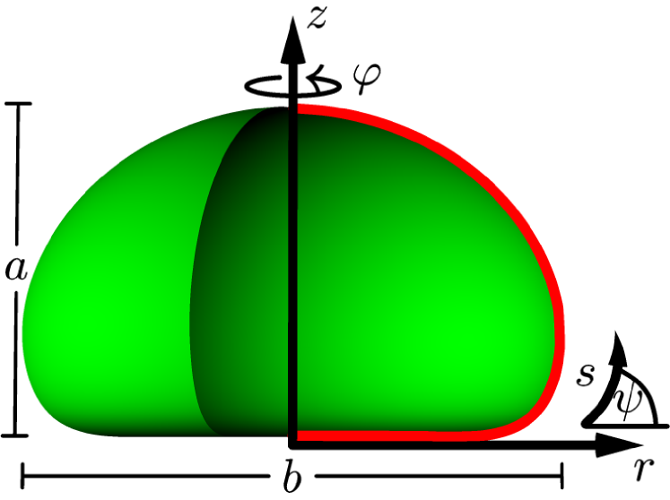
Figure 12: Parametrization of the axisymmetric capsule surface in cylindrical coordinates. The red contour line is calculated numerically.

We use a Hookean elastic energy density

$$\begin{split}w_{S}=\frac{1}{2}\frac{Y_{2\text{D}}}{1-\nu^{2}}(e_{s}^{2}+2\nu e_{s}e_{\varphi}+e_{\varphi}^{2})\\ +\frac{1}{2}E_{\text{B}}(K_{s}^{2}+2\nu K_{s}K_{\varphi}+K_{\varphi}^{2}).\end{split}$$ (S12)

The strains $e_{i}$ are related to the stretch factors $\lambda_{i}$ via $e_{i}=\lambda_{i}-1$ and the bending strains $K_{i}$ are related to the curvatures $\kappa_{i}$ via $K_{i}=\lambda_{i}\kappa_{i}-\kappa_{i_{0}}$. The index $s$ describes the meridional direction and $\varphi$ the circumferential direction. The index $0$ indicates the reference sphere. The bending modulus $E_{\text{B}}$ is defined via

$$E_{\text{B}}=\frac{Y_{2\text{D}}h^{3}}{12(1-\nu^{2})}.$$ (S13)

The constitutive relations

$$\tau_{s} =\frac{Y_{2\text{D}}}{1-\nu^{2}}\frac{1}{\lambda_{\varphi}}(e_{s}+\nu e_{\varphi}),$$ (S14)

$$m_{s} =E_{\text{B}}\frac{1}{\lambda_{\varphi}}(K_{s}+\nu K_{\varphi})$$ (S15)

for the ealstic stresses $\tau_{i}$ and the bending moments $m_{i}$ ($\tau_{\varphi}$ and $m_{\varphi}$ with interchanged indices) are obtained by variation of the energy density with respect to the strains.

The shape equations follow from purely geometric relations and the force and moment equilibrium in the shell, which is described by the following three equations (normal and tangential force equilibrium and moment equilibrium):

$$\begin{split}0&=(\tau_{s}+\gamma)\kappa_{s}+(\tau_{\varphi}+\gamma)\kappa_{\varphi}\\ &\quad-(p_{0}\Delta\rho gz+f_{m})+\frac{1}{r}\frac{\text{d}(rq)}{\text{d}s},\end{split}$$ (S16)

$$0 =\frac{\cos\psi}{r}\tau_{\varphi}+\kappa_{s}q-\frac{1}{r}\frac{\text{d}(r\tau_{s})}{\text{d}s},$$ (S17)

$$0 =q+\frac{1}{r}\frac{\text{d}(rm_{s})}{\text{d}s}-\frac{\cos\psi}{r}m_{\varphi}.$$ (S18)

Rearranging these equilibrium equations and geometrical relations for $r$, $z$ and $\psi$, we get a system of six differential equations, the shape equations:

$$r^{\prime}(s_{0}) =\lambda_{s}\cos\psi,$$ (S19)

$$z^{\prime}(s_{0}) =\lambda_{s}\sin\psi,$$ (S20)

$$\psi^{\prime}(s_{0}) =\lambda_{s}\kappa_{s},$$ (S21)

$$\tau^{\prime}_{s}(s_{0}) =\lambda_{s}\left(\frac{\tau_{\varphi}-\tau_{s}}{r}\cos\psi+\kappa_{s}q-p_{s}\right),$$ (S22)

$$m^{\prime}_{s}(s_{0}) =\lambda_{s}\left(\frac{m_{\varphi}-m_{s}}{r}\cos\psi-q\right),$$ (S23)

$$\begin{split}q^{\prime}(s_{0})&=\lambda_{s}\biggr{(}-\kappa_{s}(\tau_{s}+\gamma)-\kappa_{\varphi}(\tau_{\varphi}+\gamma)\\ &\quad-\frac{q}{r}\cos\psi+\,p_{0}+\Delta\rho gz+f_{m}\biggr{).}\end{split}$$ (S24)

The first three equations are geometrical relations, while the remaining three equations represent force and moment equilibrium. The pressure $p_{0}$ inside the capsule is modified by the hydrostatic pressure $\Delta\rho gz$ and the magnetic pressure $f_{m}$. This system is closed by the following relations:

$$\lambda_{s} =(1-\nu^{2})\lambda_{\varphi}\frac{\tau_{s}}{Y_{2\text{D}}}-\nu(\lambda_{\varphi}-1)+1,$$ (S25)

$$\lambda_{\varphi} =\frac{r}{r_{0}},$$ (S26)

$$K_{s} =\frac{1}{E_{\text{B}}}\lambda_{\varphi}m_{s}-\nu K_{\varphi},$$ (S27)

$$K_{\varphi} =\frac{\sin\psi-\sin\psi_{0}}{r_{0}},$$ (S28)

$$\kappa_{s} =\frac{K_{s}+\kappa_{s_{0}}}{\lambda_{s}},$$ (S29)

$$\kappa_{\varphi} =\frac{\sin\psi}{r},$$ (S30)

$$\tau_{\varphi} =\frac{Y_{2\text{D}}}{1-\nu^{2}}\frac{1}{\lambda_{s}}((\lambda_{\varphi}-1)+\nu(\lambda_{s}-1)),$$ (S31)

$$m_{\varphi} =\frac{E_{\text{B}}}{\lambda_{s}}(K_{\varphi}+\nu K_{s})$$ (S32)

We solve the closed system of six shape equations numerically with a fourth order Runge-Kutta scheme. Boundary conditions at the two poles follow from the requirement of a closed capsule and lead to a boundary value problem that is solved by employing a multiple shooting method in conjunction with the Runge-Kutta scheme.

A.2 Analysis of elastic parameters

For the spinning capsule experiments, we used the SVT 20 of the DataPhysics Instruments GmbH. We used Fluorinert 70 (FC 70) as outer phase because of its high density. The initial undeformed (quiescent) state was recorded at 2000 rpm. In Figure 13, a sketch of the spinning capsule measurement technique is shown.

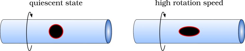
Figure 13: Spinning capsule experiment.

Capsule compression experiments were performed with the DCAT11 tensiometer (DataPhysics Instruments GmbH) with the respective software SCAT. The compression speed was set to $0.02\,\mathrm{mm}/\mathrm{s}$. A sketch of the capsule compression method is shown in Figure 14.

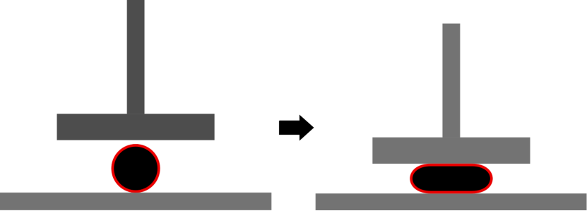
Figure 14: Capsule compression experiment.

A.3 Measurement of initial radius $R_{0}$ and volume $V_{0}$ of capsules

The radius $R_{0}$ of the initial undeformed spheres can not be measured directly, because the capsules are deformed by gravity even without an external magnetic field. Therefore, we determine the capsules’ volume from the experimental images. The image analysis was performed with FIJI/ImageJ Schindelin et al. (2012); Rueden et al. (2017)) using capsule photos taken with a OCA20 pendant drop tensiometer (DataPhysics Instruments GmbH).

In order to determine the volume $V_{0}$, we measure the axial radius $r_{i}$ at different heights $z_{i}$ and calculate $V_{0}=\int dz\pi r^{2}(z)\approx\sum_{i}\pi r_{i}^{2}(z_{i+1}-z_{i})$ by summation over small cylindrical volumes of radius $r_{i}$ at height $z_{i}$. We then calculate the initial radius by $R_{0}=(3/(4\pi)V_{0})^{(1/3)}$. We only assume that capsules are axisymmetric, which is fulfilled to a good approximation.

We find that the volume inside the capsule is constant during the whole experiment. The elastic shell is impermeable for the involved fluids.

A.4 Scanning electron microscopy (SEM) images

In order to estimate the shell thickness, SEM measurements were performed. The resulting images are shown in Figure 15. The capsule was broken prior to the measurement to avoid bursting in ultra high vacuum.

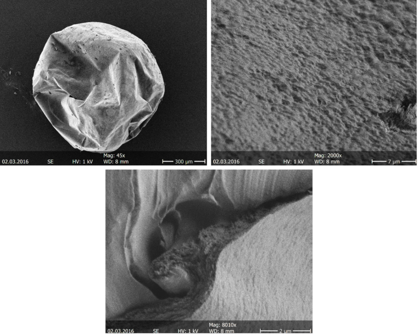
Figure 15: Scanning electron microscopy images of the ferrofluid-filled capsules. Center: complete capsule, bottom right: outer capsule shell. Top left, top right and bottom left: cross sections through ruptured parts of the shell at increasing megnification; yellow lines measure shell thickness.

This gives only a rough estimate of the thickness of the capsule shell. In addition to potential errors due to optical effects like parallax error it has to be taken into account that SEM is performed in vacuum, i.e., in the dried unhydrated state. With our optical microscope we were not able to resolve the hydrated shell of intact capsules, from which we can conclude that the shell thickness of the hydrated capsules has to be below $5\,\mathrm{\mu m}$. From the SEM images we find a shell thickness of approximately $600\,\mathrm{nm}$ in vacuum in the dried state, see yellow lines in Figure 15. For alginate capsules with thicker shells we could perform both optical microscopy measurements in the hydrated state and SEM measurements in the dried state. These measurements suggest swelling factors larger than $5$ for the thickness increase by hydration. We conclude that the shell thickness in the hydrated state is approximately $3\,\mathrm{\mu m}$ with a relatively high error around $1\,\mathrm{\mu m}$.

A.5 Fit of the external magnetic field

The external magnetic field generated by a coil with a conical iron core was measured with a hall probe. The field was measured on different positions on the central axis over the iron core and in the vicinity of the axis.

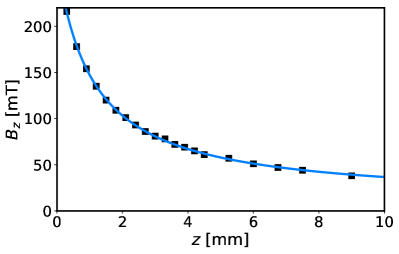
Figure 16: Magnetic flux density $B_{z}$ in $z$-direction as a function of the vertical distance $z$ to the iron core for $I=2$ A (left) and as a function of the current $I$ in the coil for $z=3.6$ mm (right). The fit eq S33 is shown as solid lines.

We found that the field was nearly constant in radial direction within a distance of about $2$ mm next to the central axis. Our biggest capsule had a radius of $R_{0}=1.044$ mm and even in the deformed state, its radial dimension did not exceed $1.4$ mm. So it is well justified to treat the magnetic field as constant in radial ($r$-) direction and to set the radial component of the field $B_{r}$ to zero. Together with the cylindrical symmetry of the setup, we only have to estimate the $z$-component $B_{z}$ that depends on the coordinate $z$ and the current $I$. We use a Langevin function to model the current dependency and a hylerbolic function for the position dependency. The measured magnetic field is in good agreement with a fit

$$B_{z}(z,I)=a\left(\coth(b_{I}I)-\frac{1}{b_{I}I}\right)\left(\frac{a_{z}}{z-b_{z}}+c_{z}\right)$$ (S33)

with parameters

$$a =4.647$$ (S34)

$$b_{I} =0.332\,\frac{1}{\text{A}}$$ (S35)

$$a_{z} =286.7\cdot 10^{-6}\,\text{Tm}$$ (S36)

$$b_{z} =-1.104\cdot 10^{-3}\,\text{m}$$ (S37)

$$c_{z} =10.86\cdot 10^{-3}\,\text{T}.$$ (S38)

The fit describes the magnetic field with an error below 1 % in the neighborhood of the capsule. A plot of the $z$- and $I$-dependence of the $B_{z}$ is shown in Figure 16.

A.6 Dynamic light scattering

To ensure the stability of the nanoparticles inside the ferrofluid dynamic light scattering measurements were performed. We used the ZetaSizer Nano ZS by Malvern instruments with the Zetasizer Software 7.12. The results were analysed with the CONTIN fit. All particle size values are given as the so-called number mean.

The capsules were produced by formation in a layer of distilled water followed by sinking into layer of aqueous sodium alginate solution (1%_w). The polymerisation time needed for the formation of stable, ferrofluid-filled capsules was 30 s. The procedure is shown in Figure 1 in the main text.

A.7 Additional interface tension in capsule compression experiments

The original Reissner formula

$$F=\frac{4Y_{2\text{D}}h}{R_{0}\sqrt{3(1-\nu^{2})}}\>d$$ (S39)

for the force-displacement relation describes the linear response of an unpressurized and initially tension-free elastic shell with rest radius $R_{0}$ to a point force $F$ in terms of the resulting indentation $d$. In the presence of an additional interfacial tension, the main difference to the purely elastic shell is a non-vanishing pressure $p_{0}$, which is caused by the interfacial tension already in the initial state with $F=0$ and which satisfies the Laplace-Young equation

$$2\gamma/R_{0}=p_{0}.$$ (S40)

We generalize Reissner’s linearized shallow shell theory Reissner (1946a, b) to include the interfacial tension and the resulting internal pressure $p_{0}$ (in Ref. 10 the related problem of pressurized shells in the absence of an interfacial tension has been considered). This leads to a linearized shallow shell equation

$$\kappa_{B}\nabla^{4}w-\gamma\nabla^{2}w+\frac{Y_{2\text{D}}}{R_{0}^{2}}w=-\frac{F}{2\pi}\frac{\delta(r)}{r}$$ (S41)

for the normal displacement $w(r)$ in polar coordinates, with $r$ as the radial distance from the origin where the point force $F$ is applied; $\kappa_{B}$ is the shell’s bending modulus

$$\kappa_{B}=\frac{Y_{2\mathrm{D}}h^{2}}{12(1-\nu^{2})}.$$ (S42)

Equation (S41) is identical to the linearized shallow shell equation governing the indentation of pressurized shells with internal pressure $p_{0}$ in the absence of interfacial tension (eq (3.2) in Ref. 10) with the interfacial tension $\gamma=p_{0}R_{0}/2$ (according to Laplace-Young equation S40) replacing the pressure-induced isotropic stress $\sigma_{\infty}=p_{0}R_{0}/2$. This means both problems are equivalent: the interfacial tension gives rise to an internal pressure $p_{0}$ in the same way as an internal pressure $p_{0}$ gives rise to an isotropic tension $\sigma_{\infty}$ prior to indentation. Consequently the solution of eq (S41) proceeds as in Ref. 10. Integrating eq (S41) The solution $w(r)$ for a given indentation $d=-w(0)$ has to be integrated over the whole reference plane of shallow shell theory to obtain the force $F=-2\pi(Y_{2\text{D}}/R_{0}^{2})\int_{0}^{\infty}drrw(r)$. This finally gives

$$F=\frac{4Y_{2\text{D}}h}{R_{0}\sqrt{3(1-\nu^{2})}}\>G(\tau)\>d$$ (S43)

with

$$G(\tau) =\frac{\pi}{2}\frac{(\tau^{2}-1)^{1/2}}{\operatorname{artanh}{(1-\tau^{-2})^{1/2}}}$$ (S44)

$$\tau =3(1-\nu^{2})\left(\gamma/Y_{2\mathrm{D}}\right)^{2}\left(R_{0}/h\right)^{2}.$$

For $\gamma\approx 0$ the Reissner result (S39) is recovered (note that in this case $\tau\approx 0$ and both the numerator and the denominator in (S44) become imaginary because $0<\tau<1$). For finite $\gamma>0$ we find a stiffening of the shell, i.e., an increased linear stiffness $F/d$ as in Ref. 10 for pressurized shells ($G(\tau)>1$ for $\tau>0$). The increase in linear stiffness remains small for $\tau\ll 1$ ($G(\tau)\approx 1$ for $\tau\ll 1$), which is fulfilled for capsule materials with $\nu$ sufficiently close to unity as for our alginate capsules. Therefore, corrections due to $\gamma>0$ remain small.

A.8 Additional interface tension in spinning drop experiments

We also have to generalize the analysis of capsule deformation in the spinning drop apparatus given in Ref. 13 in the presence of interfacial tension. The linear response of the capsule deformation in spinning drop experiments is actually equivalent to the deformation of a ferrofluid-filled capsule in a small uniform external magnetic field as it has been analyzed in Ref. 18 if we set the magnetic susceptibility to $\chi=-1$ and the magnetic field strength to $\mu_{0}H^{2}=\Delta\rho R_{0}^{2}\omega^{2}$. Both magnetic forces on the ferrofluid-filled capsule in an external field and the centrifugal pressure exerted by a liquid of different density inside the capsule are normal forces (as they are generated by liquids) acting on the capsule surface. For a spherical shape the magnetic normal forces have the same position-dependence on the polar angle (between the radial vector and the symmetry axis, i.e., field or rotation axis) for a susceptibility $\chi=-1$; for $\mu_{0}H^{2}=\Delta\rho R_{0}^{2}\omega^{2}$ also the magnitude of magnetic and centrifugal forces becomes identical. In Ref. 18 the deformation of a ferrofluid-filled magnetic capsule has already been considered also in the presence of an interfacial tension $\gamma$, and we can simply adapt the results for the linear response, which are derived in Appendix A of Ref. 18, to the capsule deformation in the spinning drop apparatus by exploiting the equivalence of both problems.

For completeness we repeat the major steps of the calculation. The linear response theory is of first order in the displacements ($u_{r},u_{\varphi},u_{\theta}$) in spherical coordinates with the polar angle $\theta$ and the azimuthal angle $\varphi$ and $\theta=0$ as the rotation axis (note that in Ref. 13 the notation is different: the azimuthal angle is denoted by $\theta$ and the polar angle by $\phi$). In the elastic shell, the equilibrium of forces has to be fulfilled in tangential and normal direction. The tangential force equilibrium is given as

$$\frac{\mathrm{d}}{\mathrm{d}\theta}(R_{0}\tau_{\theta}\sin\theta)=R_{0}\tau_{\varphi}\cos\theta$$

and the normal equilibrium as

$$\begin{split}\frac{1}{R_{0}}(\tau_{\theta}+\tau_{\varphi})+(\kappa_{\theta}+\kappa_{\varphi})\gamma\\ =p_{0}+\frac{1}{2}\Delta\rho R_{0}^{2}\omega^{2}\sin^{2}\theta.\end{split}$$

The curvatures $\kappa_{\varphi}$ and $\kappa_{\theta}$ are expanded to first order in the displacements via

$$\kappa_{\theta}+\kappa_{\varphi}\approx\frac{2}{R_{0}}-\frac{1}{R_{0}^{2}}(2u_{r}-\partial_{\theta}^{2}u_{r}+\partial_{\theta}u_{r}\cot\theta).$$

The coupled equation system describing force balance has to be solved using the constitutive relations

$$\tau_{\varphi}-\nu\tau\theta =\frac{Y_{2\mathrm{D}}}{R_{0}}(u_{\theta}\cot\theta+u_{r})$$

$$\tau_{\theta}-\nu\tau\varphi =\frac{Y_{2\mathrm{D}}}{R_{0}}(\partial_{\theta}+u_{r})$$

and the boundary conditions $\partial_{\theta}u_{r}(0)=\partial_{\theta}u_{r}(\pi/2)=0$ and $u_{\theta}(0)=u_{\theta}(\pi/2)=0$. The ansatz

$$u_{r} =A+B\cos^{2}\theta$$

$$u_{\theta} =C\sin\theta\cos\theta,$$

describes a spheroidal shape, preservation of volume requires $A=-B/3$. Using this spheroidal ansatz we find the solution

$$A =\frac{\Delta\rho R_{0}^{4}\omega^{2}(5+\nu)}{24[Y_{2\mathrm{D}}+(5+\nu)\gamma]}$$

$$B =-3A$$

$$C =\frac{\Delta\rho R_{0}^{4}\omega^{2}(1+\nu)}{4[Y_{2\mathrm{D}}+(5+\nu)\gamma]}.$$

To calculate the deformation parameter $D$, we use $r(\theta)=R_{0}+u_{r}$ and find

$$D =\frac{r(0)-r(\pi/2)}{r(0)+r(\pi/2)}$$

$$\approx\frac{B}{2R_{0}}=\frac{-\Delta\rho R_{0}^{4}\omega^{2}(5+\nu)}{16[Y_{2\mathrm{D}}+(5+\nu)\gamma]}.$$ (S45)

For $\gamma\approx 0$ we recover the well-known result from Ref. 13,

$$D=-\Delta\rho\omega^{2}R_{0}^{3}\frac{(5+\nu)}{16Y_{2\text{D}}},$$ (S46)

This means that, in the presence of an interfacial tension $\gamma>0$, we simply have to replace $Y_{2\text{D}}$ in eq S46 by $Y_{2\text{D}}+(5+\nu)\gamma$ resulting in a reduction of the deformation $D$. Analyzing the same experimental spinning capsule deformation data should give identical values of $Y_{2\mathrm{D}}+(5+\nu)\gamma$. Analyzing the same data assuming $\gamma>0$ will thus reduce the inferred result for the Young’s modulus by $(5+\nu)\gamma$.

Including an interfacial tension $\gamma$ into the combined analysis of spinning drop and capsule compression experimental data thus results in a reduced elastic modulus $Y_{2\mathrm{D}}\to Y_{2\text{D}}-(5+\nu)\gamma$ to fit the spinning drop data with eq (S45). If $\gamma/Y_{2\text{D}}\ll 1$ such that $\tau\ll 1$ in eq (S43), $\nu$ is increased at the same time such that $Y_{2\mathrm{D}}/\sqrt{1-\nu^{2}}$ remains approximately unchanged to fit the capsule compression data with eq (S43).

A.9 Sensitivity of the capsule deformation to the Poisson number $\nu$

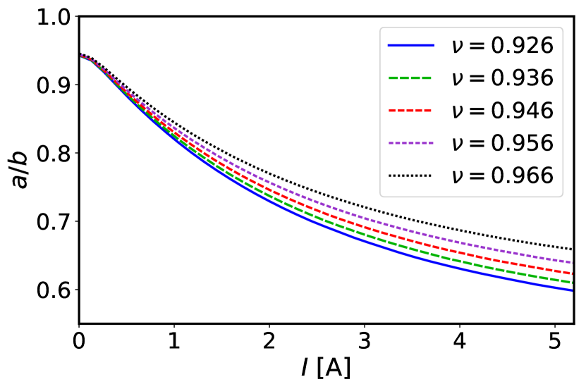
Figure 17: Ratio of the height $a$ to width $b$ of capsule 1 for increasing current $I$ with $\nu=0.926,0.936,0,946,0.956,0.966$.

A Poisson ratio close to unity gives rise to a large area compression modulus $K_{2\text{D}}=Y_{2\text{D}}/2(1-\nu)$, which becomes sensitive to changes in $\nu$ and, thus, also large elastic stresses, which contain factors $1/(1-\nu)$ and become very sensitive to changes in $\nu$ (see prefactors $1/(1-\nu^{2})$ in the elastic stresses in eq S31. Small deviations in $\nu$ lead to considerable changes in $\tau_{i}$ and visibly changing shapes of the capsule. Figure 17 shows simulations of capsule 1 with five slightly different Poisson ratios ranging from $\nu=0.926$ to $\nu=0.966$. While there are only minor deviations in the weakly deformed state in the absence of magnetic fields ($I=0\,$A), where the capsule is only deformed by gravity and tensions are dominated by the $\nu$-independent interface tension, the capsule’s side ratio $a/b$ shows obvious differences in the strongly deformed state ($I=5\,$A), which is dominated by large elastic tensions. In conclusion, strongly deformed shapes are better suited to determine the value of $\nu$. We can estimate the error of the numerically determined value of $\nu$ to be smaller than $0.01$.

A.10 List of chemicals

All chemicals including purity are shown in table 3. All chemicals were used without further purification.

Table 3: List of chemicals

Chemical	Manufacturer	Quality
Calcium chloride anhyd.	Merck	98%
Chloroform	Merck	p. A.
Diphenyl ether	Acros Organics	99%
Ethanol	VWR	99,5%
Fluorinert (FC-70)	abcr	-
$n$-Hexane	Merck	$\geq$96%
1-Hexanol	Merck	$\geq$ 98%
1,2-Hexadecanediol	Sigma Aldrich	90%
Iron acetyl acetonate	Alfa Aesar	-
Oleic acid	VWR	81%
Oleylamine	Sigma Aldrich	70%
Sodium alginata	Aldrich	-
Sodium chloride	VWR	-

References

- Rosenweig (1985) R. E. Rosenweig, Ferrohydrodynamics (Cambridge University Press, Cambridge, 1985).
- Voltairas et al. (2001) P. Voltairas, D. Fotiadis, and C. Massalas, J. Magn. Magn. Mater. 225, 248 (2001).
- Holligan et al. (2003) D. L. Holligan, G. T. Gillies, and J. T. Dailey, Nanotechnology 14, 661 (2003).
- Liu et al. (2007) X. Liu, M. D. Kaminski, J. S. Riffle, H. Chen, M. Torno, M. R. Finck, L. Taylor, and A. J. Rosengart, J. Magn. Magn. Mater. 311, 84 (2007).
- Fery et al. (2004) A. Fery, F. Dubreuil, and H. Möhwald, New J. Phys. 6, 18 (2004).
- Fery and Weinkamer (2007) A. Fery and R. Weinkamer, Polymer 48, 7221 (2007).
- Zoldesi et al. (2008) C. I. Zoldesi, I. L. Ivanovska, C. Quilliet, W. G. J. L., and A. Imhof, Phys. Rev. E 78, 051401 (2008).
- Gao et al. (2001) C. Gao, E. Donath, S. Moya, V. Dudnik, and H. Möhwald, Eur. Phys. J. E 5, 21 (2001).
- Knoche and Kierfeld (2011) S. Knoche and J. Kierfeld, Phys. Rev. E 84, 046608 (2011).
- Vella et al. (2012) D. Vella, A. Ajdari, A. Vaziri, and A. Boudaoud, J. R. Soc. Interface 9, 448 (2012).
- Barthès-Biesel (2011) D. Barthès-Biesel, Curr. Opin. Colloid Interface Sci. 16, 3 (2011).
- Carin et al. (2003) M. Carin, D. Barthès-Biesel, F. Edwards-Lévy, C. Postel, and D. C. Andrei, Biotechnol. Bioeng. 82, 207 (2003).
- Pieper et al. (1998) G. Pieper, H. Rehage, and D. Barthès-Biesel, J. Colloid Interface Sci. 202, 293 (1998).
- Knoche et al. (2013) S. Knoche, D. Vella, E. Aumaitre, P. Degen, H. Rehage, P. Cicuta, and J. Kierfeld, Langmuir 29, 12463 (2013).
- Hegemann et al. (2018) J. Hegemann, S. Knoche, S. Egger, M. Kott, S. Demand, A. Unverfehrt, H. Rehage, and J. Kierfeld, J. Colloid Interface Sci. 513, 549 (2018).
- Degen et al. (2008a) P. Degen, S. Peschel, and H. Rehage, Colloid Polym. Sci. 286, 865 (2008a).
- Karyappa et al. (2014) R. B. Karyappa, S. D. Deshmukh, and R. M. Thaokar, Phys. Fluids 26, 122108 (2014).
- Wischnewski and Kierfeld (2018) C. Wischnewski and J. Kierfeld, Phys. Rev. Fluids 3, 043603 (2018).
- Loukaides et al. (2014) E. Loukaides, S. Smoukov, and K. Seffen, Int. J. Smart Nano Mater. 5, 270 (2014).
- Seffen and Vidoli (2016) K. A. Seffen and S. Vidoli, Smart Mater. Struct. 25, 065010 (2016).
- Neveu-Prin et al. (1993) S. Neveu-Prin, V. Cabuil, R. Massart, P. Escaffre, and J. Dussaud, J. Magn. Magn. Mater. 122, 42 (1993).
- Shen et al. (2003) F. Shen, C. Poncet-Legrand, S. Somers, A. Slade, C. Yip, A. M. Duft, F. M. Winnik, and P. L. Chang, Biotechnology and Bioengineering 83, 282 (2003).
- Degen et al. (2008b) P. Degen, S. Peschel, and H. Rehage, Colloid Polym. Sci. 286, 865 (2008b).
- Degen et al. (2015) P. Degen, E. Zwar, I. Schulz, and H. Rehage, J. Phys.: Condens. Matter 27, 194105 (2015).
- Martins et al. (2015) E. Martins, D. Renard, J. Davy, M. Marquis, and D. Poncelet, J. Microencapsul. 32, 86 (2015).
- Martins et al. (2017) E. Martins, D. Renard, Z. Adiwijaya, E. Karaoglan, and D. Poncelet, J. Microencapsul. 34, 82 (2017).
- Lee and Mooney (2012) K. Y. Lee and D. J. Mooney, Prog. Polym. Sci. 37, 106 (2012).
- Leong et al. (2016) J. Y. Leong, W. H. Lam, K. W. Ho, W. P. Voo, M. F. X. Lee, H. P. Lim, S. L. Lim, B. T. Tey, D. Poncelet, and E. S. Chan, Particuology 24, 44 (2016).
- Prakash (2007) S. Prakash, Artificial Cells, Cell Engineering and Therapy, Woodhead Publishing Series in Biomaterials (Woodhead Publishing Limited/CRC Press, Cambridge/Boca Raton, 2007).
- Ouwerx et al. (1998) C. Ouwerx, N. Velings, M. M. Mestdagh, and M. A. V. Axelos, Polym. Gels Networks 6, 393 (1998).
- Mørch et al. (2006) Y. A. Mørch, I. Donati, and B. L. Strand, Biomacromolecules 7, 1471 (2006).
- Zwar et al. (2018) E. Zwar, A. Kemna, L. Richter, P. Degen, and H. Rehage, J. Phys.: Condens. Matter 30, 085101 (2018).
- Sun et al. (2004) S. Sun, H. Zeng, D. B. Robinson, S. Raoux, P. M. Rice, S. X. Wang, and G. Li, J. Am. Chem. Soc. 126, 273 (2004).
- Knoche and Kierfeld (2014) S. Knoche and J. Kierfeld, Eur. Phys. J. E 37, 62 (2014).
- Mondal et al. (2015) S. Mondal, M. Phukan, and A. Ghatak, Proc. Natl. Acad. Sci. 112, 12563 (2015).
- Afkhami et al. (2010) S. Afkhami, A. J. Tyler, Y. Renardy, T. G. St. Pierre, R. C. Woodward, and J. S. Riffle, J. Fluid Mech. 663, 358 (2010).
- Costabel (1987) M. Costabel, “Symmetric methods for the coupling of finite elements and boundary elements (invited contribution),” in Mathematical and Computational Aspects, edited by C. A. Brebbia, W. L. Wendland, and G. Kuhn (Springer, Berlin, Heidelberg, 1987) pp. 411–420.
- Wendland (1988) W. L. Wendland, “On asymptotic error estimates for combined bem and fem,” in Finite Element and Boundary Element Techniques from Mathematical and Engineering Point of View, edited by E. Stein and W. Wendland (Springer, Vienna, 1988) pp. 273–333.
- Arnold and Wendland (1983) D. N. Arnold and W. L. Wendland, Math. Comput. 41, 349 (1983).
- Arnold and Wendland (1985) D. N. Arnold and W. L. Wendland, Numer. Math 47, 317 (1985).
- Ligget and Salmon (1981) J. A. Ligget and J. R. Salmon, Int. J. Numer. Meth. Eng. 17, 543 (1981).
- Lavrova et al. (2005) O. Lavrova, V. Polevikov, and L. Tobiska, Proc. Appl. Math. Mech. 5, 837 (2005).
- Lavrova et al. (2006) O. Lavrova, G. Matthies, T. Mitkova, V. Polevikov, and L. Tobiska, J. Phys.: Condens. Matter 18, S2657 (2006).
- Harris and Basaran (1993) M. T. Harris and O. A. Basaran, J. Colloid Interface Sci. 161, 389 (1993).
- Ben Messaoud et al. (2016) G. Ben Messaoud, L. Sánchez-González, L. Probst, and S. Desobry, J. Colloid Interface Sci. 469, 120 (2016).
- Leick et al. (2010) S. Leick, S. Henning, P. Degen, D. Suter, and H. Rehage, Phys. Chem. Chem. Phys. 12, 2950 (2010).
- Leick et al. (2011) S. Leick, P. Degen, and H. Rehage, Chemie Ingenieur Technik 83, 1300 (2011).
- Reissner (1946a) E. Reissner, J. Math. Phys. 25, 80 (1946a).
- Reissner (1946b) E. Reissner, J. Math. Phys. 25, 279 (1946b).
- Vonnegut (1942) B. Vonnegut, Rev. Sci. Instrum. 13, 6 (1942).
- Princen et al. (1967) H. M. Princen, I. Y. Z. Zia, and S. G. Mason, J. Colloid Interface Sci. 23, 99 (1967).
- Barthès-Biesel et al. (2002) D. Barthès-Biesel, A. Diaz, and E. Dhenin, J. Fluid Mech. 460, 211 (2002).
- Espona-Noguera et al. (2018) A. Espona-Noguera, J. Ciriza, A. Cañibano-Hernández, L. Fernandez, I. Ochoa, L. Saenz del Burgo, and J. L. Pedraz, Int. J. Biol. Macromol. 107, 1261 (2018).
- Salsac et al. (2009) A.-V. Salsac, L. Zhang, and J. Gherbezza, 19Ème Congrès Français De Mécanique , 1 (2009).
- Maki et al. (2011) Y. Maki, K. Ito, N. Hosoya, C. Yoneyama, K. Furusawa, T. Yamamoto, T. Dobashi, Y. Sugimoto, and K. Wakabayashi, Biomacromolecules 12, 2145 (2011).
- Schindelin et al. (2012) J. Schindelin, I. Arganda-Carreras, E. Frise, V. Kaynig, M. Longair, T. Pietzsch, S. Preibisch, C. Rueden, S. Saalfeld, B. Schmid, J.-Y. Tinevez, D. J. White, V. Hartenstein, K. Eliceiri, P. Tomancak, and A. Cardona, Nature Methods 9, 676 (2012).
- Rueden et al. (2017) C. T. Rueden, J. Schindelin, M. C. Hiner, B. E. DeZonia, A. E. Walter, E. T. Arena, and K. W. Eliceiri, BMC Bioinformatics 18, 529 (2017).