Long-range spin chirality dimer order in the Heisenberg chain with modulated Dzyaloshinskii-Moriya interactions

Abstract

The ground state phase diagram of a spin $S=1/2$ $XXZ$ Heisenberg chain with spatially modulated Dzyaloshinskii-Moriya (DM) interaction

$${\cal H}=\sum_{n}J\left[\left(S^{x}_{n}S^{x}_{n+1}+S^{y}_{n}S^{y}_{n+1}+\Delta S^{z}_{n}S^{z}_{n+1}\right)+(D_{0}+(-1)^{n}D_{1})\left(S^{x}_{n}S^{y}_{n+1}-S^{y}_{n}S^{x}_{n+1}\right)\right]$$

is studied using the continuum-limit bosonization approach and extensive density matrix renormalization group computations. It is shown that the effective continuum-limit bosonized theory of the model is given by the double frequency sine-Gordon model (DSG) where the frequences i.e. the scaling dimensions of the two competing cosine perturbation terms depend on the effective anisotropy parameter $\gamma^{\ast}=J\Delta/\sqrt{J^{2}+D_{0}^{2}+D_{1}^{2}}$. Exploring the ground state properties of the DSG model we have shown that the zero-temperature phase diagram contains the following four phases: (i) the ferromagnetic phase at $\gamma^{\ast}\leq-1$; (ii) the gapless Luttinger-liquid (LL) phase at $-1<\gamma^{\ast}<\gamma^{\ast}_{c1}=-1/\sqrt{2}$; (iii) the gapped composite (C1) phase characterized by coexistence of the long-range-ordered (LRO) dimerization pattern $\epsilon\sim(-1)^{n}({\bf S}_{n}{\bf S}_{n+1})$ with the LRO alternating spin chirality pattern $\kappa\sim(-1)^{n}\left(S^{x}_{n}S^{y}_{n+1}-S^{y}_{n}S^{x}_{n+1}\right)$ at $\gamma^{\ast}_{c1}<\gamma^{\ast}<\gamma^{\ast}_{c2}$; and (iv) at $\gamma^{\ast}>\gamma^{\ast}_{c2}>1$ the gapped composite (C2) phase characterized in addition to the coexisting spin dimerization and alternating chirality patterns, by the presence of LRO antiferromagnetic order. The transition from the LL to the C1 phase at $\gamma^{\ast}_{c1}$ belongs to the Berezinskii-Kosterlitz-Thouless universality class, while the transition at $\gamma^{\ast}=\gamma^{\ast}_{c2}$ from C1 to C2 phase is of the Ising type.

I Introduction

Quantum spin chains continue to be the subject of intensive studies because they serve as interesting model systems to explore strongly correlated quantum order in low dimensional magnetic systems [Mikeska_Kolezhuk, ; Broholm_et_al_08, ; Vasiliev_Volkova_18, ]. A significant fraction of current research is focused on studies of helical structures and chiral order in the frustrated quantum magnetic systems [Zviagin, ; Derzhko_1, ; Derzhko_2, ; Oshikawa_Affleck, ; YuLu_2003, ; Mahdavifar_08, ; Aristov_Maleev_00, ; Tsvelick_01, ; Starykh_08, ; Garate_Affeck_10, ; Starykh_17, ; Fazio_14, ; Mila_et-al_11, ; Langari_09, ; Mahdavifar_14a, ; Ising_DM_1, ; Ising_DM_2, ]. The key couplings, responsible for stabilization of non-collinear magnetic configurations in these systems, is the Dzyaloshinskii-Moriya (DM) interaction [DMI-1, ; DMI-2, ]

$${\cal H}_{DM}=\sum_{n}{\bf D}(n)\cdot[{\bf S}_{n}\times{\bf S}_{n+1}]\,,$$ (1)

where ${\bf D}(n)$ is an axial DM vector. The DM interaction corresponds to the antisymmetric part of exchange interaction between spin located on neighboring sites $n$ and $n+1$, it appears in a systems with broken inversion symmetry due to the spin-orbit coupling and was first introduced by I. Dzyaloshinskii on the grounds of general symmetry arguments [DMI-1, ]. Later, the spin-orbit coupling as the microscopic mechanism of the antisymmetric exchange interaction has been identified by T. Moriya [DMI-2, ].

Although the study of helical structures in antiferromagnets counts more then half of century [Dzyaloshinskii_64, ], the research activity in the field of one and quasi-one-dimensional spin-1/2 chains with DM interaction remain persistent and high during the last three decades. Effects caused by the uniform DM term or by the pure staggered DM interaction on the ground state properties of the $S=1/2$ Heisenberg chain were considered within the framework of Bethe-Ansatz solvable models [Zviagin, ], as well as using the exactly solvable limiting cases such as the $XY$ chain with uniform DM couplings [Derzhko_1, ]. Magnetic properties of the isotropic and anisotropic ($XXZ$) Heisenberg chain with staggered [Oshikawa_Affleck, ; YuLu_2003, ; Mahdavifar_08, ] and uniform [Tsvelick_01, ; Starykh_08, ; Garate_Affeck_10, ; Starykh_17, ] DM interaction has been considered using the continuum-limit bosonization approach and numerical treatment. Recently more exotic extended versions of the one-dimensional Heisenberg model, such as the completely anisotropic spin-1/2 XYZ model with DM interaction [Fazio_14, ] and the Delta-chain model with DM interaction [Mila_et-al_11, ] have been studied using the density-matrix renormalization group algorithm (DMRG) and a finite-size scaling analysis. In last years, using the exact diagonalization technique, a special attention has been given to the studies of the ground state phase diagram of finite spin chains with DM interaction based on calculation of the entanglement, for the Heisenberg [Langari_09, ; Mahdavifar_14a, ], Ising [Ising_DM_1, ] and bond-alternating Ising model [Ising_DM_2, ].

Generally, in a chain, vectors ${\bf D}(n)$ may spatially vary both in direction and magnitude, however, the symmetry restrictions based on the properties of real solid state materials usually rule out most of the possibilities and confine the majority of theoretical discussion to two principal cases – uniform DM interaction, ${\bf D}$ vector remains unchanged over the system [Zviagin, ; Aristov_Maleev_00, ; Tsvelick_01, ; Starykh_08, ] and the case of staggered DM interaction, with antiparallel orientation of ${\bf D}$ on adjacent bonds [Oshikawa_Affleck, ; YuLu_2003, ]. Exception is only the Ref. [Derzhko_2, ] where the $XY$ spin chain with random changes in the sign of DM interactions was studied.

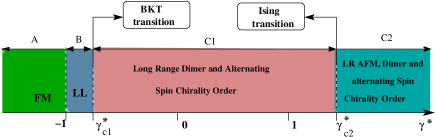
Figure 1: Sketch of the ground state phase diagram of the spin S=1/2 Heisenberg chain with modulated DM interaction.

However, recently it has been demonstrated that DM interaction can be efficiently tailored with an substantial efficiency factor by structural modulations [Geometric_tailor_DM, ] or by external electric field [EF_Enhanc_DM_1, ; EF_Enhanc_DM_2, ; EF_Enhanc_DM_3, ]. This unveils the possibility not only to control DM interaction and magnetic anisotropy via the electric field or other controllable ways, but also opens a possibility to consider effect of more general spatially modulated DM interaction on properties of the spin chain. External electric field induced modulation of the DM interaction can be realized in spin-driven chiral multiferroic (MF) systems [MF_Materials, ], effectively coupling the ferroelectric polarization with the applied external electric field [Katsura_Nagaosa_05, ]. These studies became very actual in last years, in particular in the context of materials useful for electric field controlled quantum information processing [EFC_QI_Processing, ].

In the present work we study the effect of the alternating Dzyaloshinskii-Moriya (DM) interaction on the ground state phase diagram of the spin-1/2 Heisenberg chain. Because the DM term breaks the global spin rotation symmetry, we consider the Hamiltonian

$${\cal H}={\cal H}_{XXZ}+{\cal H}_{DM}$$

where

$${\cal H_{XXZ}}=\sum_{n}\left[J(S^{x}_{n}S^{x}_{n+1}+S^{y}_{n}S^{y}_{n+1})+J_{z}\,S^{z}_{n}S^{z}_{n+1}\right]$$ (2)

is the Hamiltonian of an anisotropic Heisenberg chain and ${\cal H}_{DM}$ is the DM term given in Eq. (1). In what follows we choose the ${\bf D}(n)$ vector orientated, in the spin space, along the ${\hat{z}}$ axis ${\bf D}(n)=(0,0,D(n))$ and take

$$D(n) = D_{0}+(-1)^{n}D_{1}\,.$$ (3)

Our main objective is to show that the spatial modulation of the DM interaction leads to dramatic change of the ground state phase diagram of the system, opens a gap in a wide area of the parameter range and also changes the nature of quantum phase transition in the long-range-ordered antiferromagnetic phase. Results are summarized in the Fig. 1. The ground state phase diagram is divided into four sectors depending on the value of the effective exchange anisotropy parameter $\gamma^{\ast}=J_{z}/\sqrt{J^{2}+D_{0}^{2}+D_{1}^{2}}$. The $\gamma^{\ast}=-1$ point corresponds to the transition into the ferromagnetically ordered phase (sector A). The gapless Luttinger-liquid phase is shrunk up to a narrow region between $-1<\gamma^{\ast}<\gamma^{\ast}_{c1}=-\sqrt{2}/2$ (sector B). At $\gamma^{\ast}=\gamma^{\ast}_{c1}$ the Berezinskii-Kosterlitz-Thouless (BKT) phase transition takes the system into the composite (C1) gapped phase characterized by the coexistence of long-range ordered (LRO) alternating spin dimerization pattern

$$\epsilon(n)=\langle{\bf S}_{n}\cdot{\bf S}_{n+1}\rangle\sim const+(-1)^{n}\epsilon$$

coexisting with long-range alternating pattern of the spin chirality vector

$$\kappa^{z}_{n}=\langle\left[\,{\bf S}_{n}\times{\bf S}_{n+1}\,\right]_{z}\rangle\sim const+(-1)^{n}\kappa\,.$$

Finally, at $\gamma^{\ast}=\gamma^{\ast}_{c2}>1$ there is an Ising type phase transition into the other composite (C2) gapped phase, characterized by the coexistence of long-range dimerization, chirality and antiferromagnetic

$$\langle S_{n}^{z}\rangle\sim const+(-1)^{n}m$$

modulations.

The outline of the paper is as follows. In Sec. II we consider the exactly solvable limit case of the $XY$ chain with alternating DM interaction. In Sec. III using the gauge transformation we gauge out the DM coupling and obtain an effective $XXZ$ spin-chain Hamiltonian with alternating transverse exchange. In Sec. IV we construct the weak-coupling bosonized version of the effective Hamiltonian and discuss ground state phase diagram. In Sec. V we present extensive numerical results supporting the bosonization predictions. Finally, a brief summary is presented in Sec. VI.

II The XX chain with alternating DM interaction.

In this Section we consider the exactly solvable case of a XX chain with alternating DM interaction. It is instructive to start from the full Hamiltonian

$${\cal H} = \sum_{n}\Big{[}\frac{J}{2}\left(S^{+}_{n}S^{-}_{n+1}+S^{-}_{n}S^{+}_{n+1}\right)+J_{z}\,S^{z}_{n}S^{z}_{n+1}$$ (4)

$$+ \frac{i}{2}(D_{0}+(-1)^{n}D_{1})\left(S^{+}_{n}S^{-}_{n+1}-S^{-}_{n}S^{+}_{n+1}\right)\Big{]}\,,$$

where $S^{+}_{n}=S^{+}_{x}\pm iS^{+}_{y}$.

Using the Jordan-Wigner transformations [JW_1928, ]

$$S_{n}^{+} = a^{\dagger}_{n}\exp\left(i\pi\sum_{m<n}a^{\dagger}_{m}a^{\phantom{\dagger}}_{m}\right)\,,$$ (5)

$$\quad S_{n}^{-} = \exp\left(-i\pi\sum_{m<n}a^{\dagger}_{m}a^{\phantom{\dagger}}_{m}\right)a_{n}\,,$$ (6)

$$S^{z}_{n} = a^{\dagger}_{n}a^{\phantom{\dagger}}_{n}-1/2,$$ (7)

where $a^{\dagger}_{n}$ ($a^{\phantom{\dagger}}_{n}$) is a spinless fermion creation (annihilation) operator on site $n$, we rewrite the initial lattice spin Hamiltonian (4) in terms of interacting spinless fermions in the following way:

$${\cal H} = \frac{J}{2}\sum_{n}\left(a^{\dagger}_{n}a^{\phantom{\dagger}}_{n+1}+a^{\dagger}_{n+1}a^{\phantom{\dagger}}_{n}\right)$$ (8)

$$+ \frac{iD_{0}}{2}\sum_{n}\left(a^{\dagger}_{n}a^{\phantom{\dagger}}_{n+1}-a^{\dagger}_{n+1}a^{\phantom{\dagger}}_{n}\right)$$

$$+ \frac{iD_{1}}{2}\sum_{n}(-1)^{n}\left(a^{\dagger}_{n}a^{\phantom{\dagger}}_{n+1}-a^{\dagger}_{n+1}a^{\phantom{\dagger}}_{n}\right)$$

$$+ J_{z}\sum_{n}(a^{\dagger}_{n}a^{\phantom{\dagger}}_{n}-1/2)(a^{\dagger}_{n+1}a^{\phantom{\dagger}}_{n+1}-1/2)\,.$$

We first discuss the exactly solvable $XX$ limit $J_{z}=0$. Indeed, in absence of the Ising part of the spin exchange ($J_{z}=0$), the Hamiltonian can be easily diagonalized in the momentum space. Indeed, performing the Fourier transform,

$$a_{n} = \frac{1}{\sqrt{L}}\sum_{k}\,a_{k}e^{ikn}\,,$$ (9)

at $J_{z}=0$ we obtain

$${\cal H} = \sum_{k}\left[\epsilon(k)\,a^{\dagger}_{k}a^{\phantom{\dagger}}_{k}+i\Delta(k)a^{\dagger}_{k}a^{\phantom{\dagger}}_{k+\pi}\right]\,,$$ (10)

where

$$\epsilon(k) = \left(J\cos k-D_{0}\sin k\right)=J_{eff}\cos(k+q_{0})\,,$$ (11)

$$\Delta(k) = D_{1}\cos k$$ (12)

and

$$J_{eff} = \sqrt{J^{2}+D_{0}^{2}}$$ (13)

$$q_{0} = \arctan(D_{0}/J)\,.$$ (14)

Thus, in absence of the staggered component of the DM interaction and ($D_{1}=0$) the excitation spectrum of the model is given by the same dispersion relation as the standard $XX$ chain

$${\cal H}_{0} = \sum_{k}\epsilon(k)\,a^{\dagger}_{k}a^{\phantom{\dagger}}_{k}\,,$$ (15)

but for a uniform shift $q_{0}$ in the momentum vector due to the uniform part of the DM interaction [Derzhko_1, ]. The system is characterized by two Fermi points $k_{F}^{\pm}=\pm\frac{\pi}{2}-q_{0}$, so that in the ground state all states with $\pi/2\leq|k+q_{0}|\leq\pi$ are occupied and those with $|k+q_{0}|<\pi/2$ are empty. The bandwidth is half filled, the total magnetization of the system in the ground state as well as the average value of the on-site spin vanishes

$$m=\frac{1}{L}\sum_{n}\langle 0|S_{n}^{z}|0\rangle=0\,.$$ (16)

The vacuum spin current, determined via the chirality order parameter [Chubukov_91, ; Furusaki_08, ] is evaluated as

$$J_{sp}=\frac{1}{L}\sum_{n}\langle 0|\kappa^{z}_{n}|0\rangle=\frac{2}{\pi}\sin q_{0}\,.$$ (17)

Note that due to the gapless excitation spectrum, all corresponding correlations decay in power-laws [Takahashi_book_99, ] and no LRO is present in absence of modulated part of the DM interaction.

Figure 2: Free spinless fermion (spinon) dispersion relation in the case of finite uniform and alternating DM interaction. Here $J=1$, $J_{z}=0$, $D_{0}=\tan(\pi/6)$ and $D_{1}=0.2$

At $D_{1}\neq 0$, diagonalization of the Hamiltonian (10) is also straightforward. It is convenient to restrict momenta within the reduced Brillouin zone $-\pi/2<k\leq\pi/2$ and to introduce a new notation $a_{k+\pi}=b_{k}$. In these terms the Hamiltonian reads

$${\cal H}=\sum_{k}{}^{\prime}\left[\epsilon(k)\left(a_{k}^{{\dagger}}a^{\phantom{\dagger}}_{k}-b_{k}^{{\dagger}}b^{\phantom{\dagger}}_{k}\right)+i\Delta(k)\left(a_{k}^{{\dagger}}b^{\phantom{\dagger}}_{k}-b_{k}^{{\dagger}}a^{\phantom{\dagger}}_{k}\right)\right]\,,$$

where prime in the sum means that the summation is taken over the reduced Brilluoin zone $-\pi/2<k\leq\pi/2$. Using the unitary transformation

$$a_{k} = \cos\phi_{k}\,\alpha_{k}+i\sin\phi_{k}\,\beta_{k}\,,$$ (18)

$$b_{k} = i\sin\phi_{k}\,\alpha_{k}+\cos\phi_{k}\,\beta_{k}\,.$$ (19)

and choosing

$$\tan\left(2\phi_{k}\right)=-\Delta(k)/\epsilon(k)$$

we obtain

$${\cal H} = \sum_{\pi/2<k\leq\pi/2}E(k)\left(\alpha_{k}^{{\dagger}}\alpha^{\phantom{\dagger}}_{k}-\beta_{k}^{{\dagger}}\beta^{\phantom{\dagger}}_{k}\right)$$ (20)

where

$$E(k) = \sqrt{J^{2}_{eff}\cos^{2}(k+q_{0})+D_{1}^{2}\cos^{2}k}$$ (21)

Note that in absence of the uniform component of the DM interaction ($D_{0}=0,\,D_{1}\neq 0$), $E(k)=\pm\sqrt{J^{2}+D_{1}^{2}}\,\cos k$ and therefore the excitation spectrum is gapless, the vacuum spin current $J_{sp}=0$ and no LRO is present in the ground state.

Only at $D\neq 0,\,D_{1}\neq 0$ the spectrum is characterized by a finite excitation gap (see Fig. 2).

$$\Delta_{exc} = J^{\ast}\sqrt{2\left(1-\sqrt{1-\left(2D_{0}D_{1}/J^{\ast}\right)^{2}}\right)}$$ (22)

$$\hskip 22.76219pt\simeq 2D_{0}\,D_{1}/J^{\ast}\,,$$

where

$$J^{\ast}=\sqrt{J^{2}+D^{2}_{0}+D^{2}_{1}}\,.$$

In the ground state of the gapped phase, all states in the negative energy $\beta$-band are filled $n_{\beta}(k)=\langle\beta^{\dagger}_{k}\beta^{\phantom{\dagger}}_{k}\rangle=1$, while all the states in the positive energy $\alpha$-band are empty, $n_{\alpha}(k)=\langle\alpha^{\dagger}_{k}\alpha^{\phantom{\dagger}}_{k}\rangle=1$. As the result, in the ground state the $z$-projection of the total spin

$$M=\sum_{n}\langle 0|S_{n}^{z}|0\rangle=\frac{L}{2\pi}\int_{-\pi/2}^{\pi/2}[\,n_{\beta}(k)-1/2\,]=0\,$$ (23)

as well as the staggered part of the on-site magnetization

$$m=\frac{1}{L}\sum_{n}(-1)^{n}\langle 0|S_{n}^{z}|0\rangle=0\,.$$ (24)

It is straightforward to obtain, that the ground state average of the staggered transverse spin dimerization and chirality order parameters [Chubukov_91, ; Furusaki_08, ] are given by

$$\epsilon_{\perp} = \frac{1}{L}\sum_{n}\,(-1)^{n}\langle 0|\left(S^{+}_{n}S^{-}_{n+1}+S^{-}_{n}S^{+}_{n+1}\right)|0\rangle=$$ (25)

$$= -\frac{D_{1}}{\pi}\int_{-\pi/2}^{\pi/2}\,\frac{\sin k\cos k}{E(k)}\,dk\,$$

and

$$\kappa = \frac{i}{L}\sum_{n}\,(-1)^{n}\langle 0|\left(S^{+}_{n}S^{-}_{n+1}-S^{-}_{n}S^{+}_{n+1}\right)|0\rangle=$$ (26)

$$= \frac{D_{1}}{\pi}\int_{-\pi/2}^{\pi/2}\,\frac{\cos^{2}k}{E(k)}\,dk\,.$$

respectively.

It is easy to check by inspection, that both link-located order parameters $\epsilon_{\perp}\rightarrow 0$ and $\kappa\rightarrow 0$ at $D_{0}=0$ and $D_{1}\neq 0$.

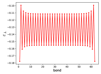
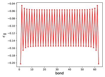
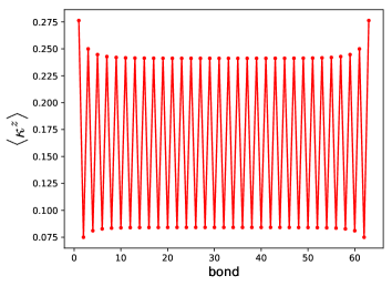
Figure 3: The ground state expectation value distribution along bonds of: the transverse part of the nearest-neighbor spin-spin exchange operator $\epsilon_{n}^{\perp}$ (top panel), the longitudinal part of the same operator $\epsilon_{n}^{\parallel}$ (middle panel), and the spin chirality operator $\kappa^{z}_{n}$ (bottom panel) in the case of finite uniform and alternating DM interactions. The results correspond to a chain of $L=64$ sites with OBC, with parameters $J=1$, $D_{0}=\tan(\pi/6)$ and $D_{1}=0.2$.

To conclude the considerations on the $XX$ limit of the model (2), we present exact results of the local ground state expectation values of the considered order parameters, aiming to illustrate the described ordered patterns. They have been obtained for finite chains of length $L=64$ with open boundary conditions (OBC), also providing an insight into boundary features found in DMRG computations for the interacting case (see Section V).

In Fig. 3 we have plotted the ground state distribution of the transverse and longitudinal components of the spin-exchange

$$\epsilon_{\perp}(n) = \frac{1}{2}\langle\left(S^{x}_{n}S^{x}_{n+1}+S^{y}_{n}S^{y}_{n+1}\right)\rangle\,,$$ (27)

$$\epsilon_{\parallel}(n) = \langle\,S^{z}_{n}S^{z}_{n+1}\,\rangle\,,$$ (28)

and that of the $z$-component of the spin chirality vector, $\kappa^{z}_{n}$. These show a well pronounced alternating pattern in complete agreement with analytical results. Notice that distortions close to the edges are a byproduct of OBC, thus in order to compute bulk averages one usually discards a convenient number of sites at each boundary.

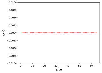
Figure 4: The ground state expectation value distribution of the $z$ component of the spin operator as a function of site number. System parameters are the same as in Fig. 3.

In Fig. 4 we show the ground state distribution of the on-site magnetization. In spite of the modulated terms in the Hamiltonian one observes that the $z$-component of the spin density is homogeneous and strongly zero, in marked contrast with the ground state averages of the link-located order parameters.

III Gauging away the DM interaction

To make next step forward, it is useful to rewrite the Hamiltonian (4) in a physically more suggestive manner by rotating spins and gauging away the DM interaction term. Here we follow the route, developed in the Ref. [Tsvelick_01, ], in the case of a chain with uniform DM interaction.

In the considered case of the Heisenberg chain with alternating DM interaction, as a first step it is convenient to rewrite the Hamiltonian in a way which explicitly takes into account doubling of the unit cell by the staggered part of the DM interaction. Defining new dimensionless parameters $d_{\pm}=(D_{0}\pm D_{1})/J$ the Hamiltonian (2) reads

$${\cal H} = \frac{J}{2}\sum_{m=1}^{N/2}\Big{[}\,\left(S^{+}_{2m-1}S^{-}_{2m}+S^{-}_{2m-1}S^{+}_{2m}\right)$$ (29)

$$+ i\,d_{-}\left(S^{+}_{2m-1}S^{-}_{2m}-S^{-}_{2m-1}S^{+}_{2m}\right)$$

$$\hskip 14.22636pt+\left(S^{+}_{2m}S^{-}_{2m+1}+S^{-}_{2m}S^{+}_{2m+1}\right)$$

$$+ i\,d_{+}\left(S^{+}_{2m}S^{-}_{2m+1}-S^{-}_{2m}S^{+}_{2m+1}\right)$$

$$\hskip 14.22636pt+2\,\Delta\,S^{z}_{2m}\left(S^{z}_{2m-1}+S^{z}_{2m+1}\right)\Big{]}\,.$$

We introduce new spin variables ${\bf\tau}_{2m}$ and ${\bf\tau}_{2m+1}$ by performing a site-dependent rotation of spins along the chain around the $z$ axis with relative angle $\vartheta_{-}$ for spins at consecutive odd-even sites ($2m-1,2m$) and $\vartheta_{+}$ for spins at consecutive even-odd sites ($2m,2m+1$), so that

$$S^{+}_{2m-1}=e^{i(m-1)(\vartheta_{-}+\vartheta_{+})}\,\,\tau^{+}_{2m-1}\,,$$

$$S^{+}_{2m}=e^{im\vartheta_{-}+i(m-1)\vartheta_{+}}\,\,\tau^{+}_{2m}\,,$$ (30)

$$S^{+}_{2m+1}=e^{im(\vartheta_{-}+\vartheta_{+})}\,\,\tau^{+}_{2m+1}\,,$$

$$S^{z}_{2m\pm 1}=\tau^{z}_{2m\pm 1}\,\qquad S^{z}_{2m}=\tau^{z}_{2m}\ .$$

In the new variables we obtain

$$S_{2m-1}^{+}S_{2m}^{-}\,\pm h.c. = \cos\vartheta_{-}\left(\tau_{2m-1}^{+}\tau_{2m}^{-}\,\pm\,\tau_{2m-1}^{-}\tau_{2m}^{+}\right)$$ (31)

$$-i\sin\vartheta_{-}\left(\tau_{2m-1}^{+}\tau_{2m}^{-}\,\mp\,\tau_{2m-1}^{-}\tau_{2m}^{+}\right),$$

$$S_{2m}^{+}S_{2m+1}^{-}\,\mp\,h.c. = \cos\vartheta_{+}\left(\tau_{2m}^{+}\tau_{2m+1}^{-}\,\pm\,\tau_{2m}^{-}\tau_{2m_{1}}^{+}\right)$$ (32)

$$-i\sin\vartheta_{+}\left(\tau_{2m}^{+}\tau_{2m+1}^{-}\,\mp\,\tau_{2m}^{-}\tau_{2m+1}^{+}\right).$$

Inserting (31)-(32) in (29) we map the initial Hamiltonian onto

$${\cal H}=\frac{J}{2}\sum_{m=1}^{N/2}\Big{[}\,\left(\cos\vartheta_{-}+d_{-}\sin\vartheta_{-}\right)\left(\tau_{2m-1}^{+}\tau_{2m}^{-}+\tau_{2m}^{-}\tau_{2m-1}^{+}\right)$$

$$\hskip 11.38109pt-i\,\left(\sin\vartheta_{-}-d_{-}\cos\vartheta_{-}\right)\left(\tau_{2m-1}^{+}\tau_{2m}^{-}\,-\,\tau_{2m}^{-}\tau_{2m-1}^{+}\right)$$

$$\hskip 11.38109pt\,+\left(\cos\vartheta_{-}+d_{+}\sin\vartheta_{+}\right)\left(\tau_{2m}^{+}\tau_{2m+1}^{-}\,+\,\tau_{2m}^{-}\tau_{2m+1}^{+}\right)$$

$$\hskip 11.38109pt-i\left(\sin\vartheta_{-}-d_{+}\cos\vartheta_{+}\right)\left(\tau_{2m}^{+}\tau_{2m+1}^{-}\,-\,\tau_{2m}^{-}\tau_{2m+1}^{+}\right)$$

$$\hskip 11.38109pt+2\,\Delta\,\tau_{2m}^{z}\,\left(\tau_{2m-1}^{z}+\tau_{2m+1}^{z}\right)\Big{]}\,.$$ (33)

Choosing angles $\vartheta_{\pm}$ such that

$$\tan\vartheta_{\pm}=d_{\pm},$$

one can cancel DM like terms

$$J(\sin\vartheta_{\pm}-d_{\pm}\,\cos\theta_{\pm})=0\,,$$

$$J(\cos\vartheta_{\pm}+d_{\pm}\,\sin\theta_{\pm})=J\sqrt{1+d_{\pm}^{2}}\,\equiv J_{\pm}$$ (34)

and obtain the Hamiltonian without the DM interaction but only with the alternating transverse exchange interaction [Derzhko_2, ]

$${\cal H} = \sum_{m=1}^{N/2}\Big{[}\,\frac{J_{-}}{2}\left(\tau^{+}_{2m-1}\tau^{-}_{2m}+\tau^{-}_{2m-1}\tau^{+}_{2m}\right)$$ (35)

$$\hskip 14.22636pt+\,\frac{J_{+}}{2}\left(\tau^{+}_{2m}\tau^{-}_{2m+1}+\tau^{-}_{2m}\tau^{+}_{2m+1}\right)$$

$$\hskip 14.22636pt+\,J_{z}\,\tau^{z}_{2m}\left(\tau^{z}_{2m-1}+\tau^{z}_{2m+1}\right)\Big{]}\,.$$

It is instructive to rewrite the Hamiltonian (35) in the following, more common, form

$${\cal H} = \tilde{J}\sum_{n}\Big{[}\,\frac{1}{2}(1+(-1)^{n}\delta)\left(\tau^{+}_{n}\tau^{-}_{n+1}+\tau^{-}_{n}\tau^{+}_{n+1}\right)$$ (36)

$$\hskip 34.1433pt\,+\gamma^{\ast}\tau^{z}_{n}\tau^{z}_{n+1}\Big{]}\,,$$

where, at $d_{i}\ll 1$ ( $i=\pm$),

$$\tilde{J}=\frac{1}{2}\left(J_{+}+J_{-}\right)\simeq J^{\ast}+{\cal O}\left(d_{i}^{4}\right),$$ (37)

$$\delta\,\tilde{J}=\frac{1}{2}\left(J_{+}-J_{-}\right)\simeq\frac{D_{0}D_{1}}{J^{\ast}}+{\cal O}\left(d_{i}^{4}\right)\,$$ (38)

and

$$\gamma^{\ast}=J_{z}/\tilde{J}\simeq J_{z}/J^{\ast}+{\cal O}\left(d_{i}^{4}\right)\,.$$ (39)

At $J_{-}\neq J_{+}$ the Hamiltonian (36) is recognized as a Hamiltonian of the $XXZ$ chain with alternating transverse exchange. Note that the alternation of the transverse exchange $\delta\neq 0$ only for finite $D_{1}\neq 0$ and $D_{0}\neq 0$. In the following we will discard ${\cal O}\left(d_{i}^{4}\right)$ corrections.

In the case of uniform DM interaction ($D_{1}=0$) the gauge transformation reduces to the consecutive rotation of spins along the chain around the $z$ axis with respect to the nearest neighbor on the same angle

$$\theta=\arctan\left(D_{0}/J\right).$$

Because in this limit $J_{+}=J_{-}$ i.e. $\delta=0$, the effect of the uniform DM interaction reduces to the renormalization of the exchange anisotropy $\gamma\rightarrow\gamma^{\ast}$ and change of the boundary conditions. Respectively the Heisenberg chain with uniform DM interaction is equivalent to an XXZ chain with twisted boundary conditions. In particular, the excitation spectrum and the bulk correlation functions of a spin-1/2 XXZ Heisenberg chain with DM interaction can be obtained from that of the corresponding XXZ chain

$${\cal H}=J^{\ast}\sum_{n=1}^{N}\Big{[}\,\frac{1}{2}\left(\tau^{+}_{n}\tau^{-}_{n+1}+\tau^{-}_{n}\tau^{+}_{n+1}\right)+\gamma^{\ast}\tau^{z}_{n}\tau^{z}_{n+1}\Big{]},$$ (40)

taking into account the shift in momentum induced by the mapping (30) and renormalization of the anisotropy parameter [Tsvelick_01, ].

In the case of staggered DM interaction $D(n)=(-1)^{n}D_{1}$

$$\vartheta_{+}=-\vartheta_{-}=\vartheta=\arctan\left(D_{1}/J\right)$$

and the gauge transformation becomes global and corresponds to the rotation of all spins on even sites around the $z$ axis on the same angle $\theta$

$$S^{+}_{2m} = e^{i\theta}\,\tau^{+}_{2m},\,S^{z}_{2m}=\tau^{z}_{2m+1}\ ,$$ (41)

while the spins on even sites remain untouched:

$$S^{+}_{2m-1} = \tau^{+}_{2m-1},\,S^{z}_{2m}=\tau^{z}_{2m}.$$ (42)

This gives again the Hamiltonian (40), but with transverse exchange

$$J^{\ast}=\sqrt{J^{2}+D_{1}^{2}}\,.$$

Thus the effect of staggered DM interaction reduces only to the enhancement of the exchange anisotropy and to the renormalization of the bandwidth without any influence on the character of the spectrum. For a system with open boundary conditions there are no further changes, except for the appearance of gapless topological edge states [SSH_79, ] that we take apart in numerical computations. The bulk correlation functions of a spin-1/2 Heisenberg chain with staggered DM interaction can be obtained from that of the corresponding XXZ chain (40) by taking into account the shift on the relative angle $\theta$ between spins located on even and odd sites.

The next step is to incorporate the effect of longitudinal part of the spin exchange. Below we use the continuum-limit bosonization approach to study low-energy properties of the Hamiltonian (36).

IV The continuum-limit bosonization approach

The continuum-limit bosonization approach to spin chains is well known and discussed in detail in many excellent reviews and books. Therefore, below we briefly sketch the most relevant steps and bosonization conventions, while for technical details we refer the reader to the corresponding references [Affleck_LN, ; GNT_Book, ; Giamarchi_Book, ].

To obtain the continuum version of the Hamiltonian (40), we use the standard bosonization expression of the spin operators [GNT_Book, ]

$$\tau_{n}^{z} \simeq \sqrt{\frac{K}{\pi}}\partial_{x}\phi(x)+(-1)^{n}\frac{{\it a}}{\pi\alpha}\sin\sqrt{4\pi K}\phi(x)\,,$$ (43)

$$\tau^{\pm}_{n} \simeq \frac{{\it b}}{\pi\alpha}\cos(\sqrt{4\pi K}\phi)\,e^{\pm i\sqrt{\pi/K}\theta}$$ (44)

$$- (-1)^{n}\frac{{\it c}}{\pi\alpha}\,e^{\pm i\sqrt{\pi/K}\theta}\,.$$

Here $\phi(x)$ and $\theta(x)$ are dual bosonic fields, $\partial_{t}\phi=u\partial_{x}\theta$, and satisfy the following commutational relation

$$[\phi(x),\theta(y)]=i\Theta(y-x)\,,$$

$$[\phi(x),\theta(x)]=i/2\,.$$ (45)

Here the non-universal real constants a, b and c depend smoothly on the parameter $\gamma^{\ast}$, are of the order of unity at $\gamma^{\ast}=0$ [Hikihara_Furusaki_98, ; Lukyanov_Terras_03, ] and are expected to be nonzero everywhere at $|\gamma^{\ast}|<1$. The Luttinger liquid parameter is known within the critical line $-1<\gamma^{\ast}<1$ to be [LP_75, ]

$$K = \frac{\pi}{2\arccos\left(-\gamma^{\ast}\right)}\,.$$ (46)

Thus the parameter $K$ decreases monotonically from its maximal value $K\to\infty$ at $\gamma^{\ast}\to-1$ (ferromagnetic instability point), is equal to unity at $\gamma^{\ast}=0$ ($J_{z}=0$) and reaches the value $K=1/2$ at $\gamma^{\ast}=1$ (isotropic antiferromagnetic chain). In the case of dominating Ising type anisotropy, at $\gamma^{\ast}>1$, $K<1/2$.

Using (43)-(44) we finally obtain for the initial lattice Hamiltonian (35):

$${\cal H} = u\int dx\,\Big{[}\frac{1}{2}(\partial_{x}\phi)^{2}+\frac{1}{2}(\partial_{x}\theta)^{2}+\frac{m_{0}}{\pi\alpha^{2}}\cos\sqrt{4\pi K}\phi$$ (47)

$$\hskip 51.21495pt+\frac{M_{0}}{\pi\alpha^{2}}\cos\sqrt{16\pi K}\phi\,\Big{]}\,,$$

where

$$m_{0} \simeq \delta=D_{0}D_{1}/J^{\ast\,2}\,,$$ (48)

$$M_{0} \simeq \gamma^{\ast}/2\pi$$ (49)

and $u\simeq J^{\ast}/K$ stands for the velocity of spin excitation. Thus the effective continuum-limit version of the initial lattice spin model (35) is given by the double-frequency sine-Gordon (DSG) model [DSG_Book_80, ]. The DSG model (47) describes an interplay between two perturbations to the Gaussian conformal field theory with the ratio of their scaling dimensions equal to four. The DSG model and its realizations in various 1D systems have been subject of intensive studies in last decades [DSG_1, ; DSG_2a, ; DSG_2b, ; DSG_3a, ; DSG_3b, ; DSG_4, ; DSG_5, ; DSG_6, ; JN_19, ]. It has been shown [DSG_1, ], that the ground state properties of the DSG model are controlled by the scaling dimensions of the two cosine terms

$$d=dim[\cos\sqrt{4\pi K}\phi]=K$$

and

$$d^{\ast}=dim[\cos\sqrt{16\pi K}\phi]=4K\,$$

present in the Hamiltonian. Each of these cosine terms becomes relevant in the parameter range where the corresponding scaling dimensionality $d\leq 2$ or $d^{\ast}\leq 2$. Using (46) we find that $d\leq 2$, i.e. the first cosine term in (47) is relevant, at $\gamma^{\ast}>\gamma^{\ast}_{c1}=-\sqrt{2}/2$, while $d^{\ast}\leq 2$, i.e. the second cosine term in (47), for $\gamma^{\ast}>1$. This gives following four segments of the model parameter range (see Fig. 1), where each one corresponds to the different mechanisms of formation of the ground-state properties of the system:

IV.1 The Ferromagnetic sector $\gamma^{\ast}\leq-1$

At $\gamma^{\ast}\leq-1$ the system is in the ferromagnetic phase, all spins are oriented along the z-axis

$$\langle\tau_{n}^{z}\rangle=\langle S_{n}^{z}\rangle=1/2;\\ \langle\tau_{n}^{x}\rangle=\langle\tau_{n}^{y}\rangle=0$$

and therefore the effect of the DM interaction is completely suppressed.

IV.2 The Luttinger-liquid sector $-1<\gamma^{\ast}<\gamma^{\ast}_{c1}$

At $-1<\gamma^{\ast}<\gamma^{\ast}_{c1}$, $d^{\ast}>d>2$ and therefore both cosine terms in (47) are irrelevant and can be neglected. The gapless long-wavelength excitations of the anisotropic spin chain are described by the standard Gaussian theory with the Hamiltonian

$${\cal H}_{0} = u\int dx\,\Big{[}\,\frac{1}{2}(\partial_{x}\phi)^{2}+\frac{1}{2}(\partial_{x}\theta)^{2}\,\Big{]}.$$ (50)

In this critical Luttinger-liquid phase, all correlations show a power-law decay, with indices smoothly depending on the parameter $K$ [GNT_Book, ].

IV.3 The dimerized sector $\gamma^{\ast}_{c1}<\gamma^{\ast}\leq 1$

At $\gamma^{\ast}_{c1}<\gamma^{\ast}\leq 1$, $d<2$ while $d^{\ast}>2$, therefore the double-frequency cosine term is irrelevant and can be neglected. In this case infrared properties of the system are described by the standard sine-Gordon (SG) model

$${\cal H}=u\int dx\,\Big{[}\frac{1}{2}(\partial_{x}\phi)^{2}+\frac{1}{2}(\partial_{x}\theta)^{2}+\frac{m_{0}}{\pi\alpha^{2}}\cos\sqrt{4\pi K}\phi\Big{]}.$$ (51)

With increasing $\gamma^{\ast}$, the scaling dimensionality of the relevant cosine term changes from the marginal value $d=2$ at $\gamma^{\ast}=\gamma^{\ast}_{c1}$, to $d=1/2$ at $\gamma^{\ast}=1$. Thus, at $\gamma^{\ast}=\gamma^{\ast}_{c1}\simeq-0.7$ the BKT [KT_73, ] quantum phase transition takes place in the ground state of the system, the excitation gap opens at $\gamma^{\ast}=\gamma^{\ast}_{c1}$ and remains finite in the whole region $-0.7<\gamma^{\ast}\leq 1$.

From the exact solution of the quantum sine-Gordon model [SG_exact_Sol, ; Zamolodchikov_95, ] it is known that for arbitrary finite $m_{0}$ the gapped excitation spectrum of the Hamiltonian Eq. (51) at $2>d>1$ ($-0.7<\gamma^{\ast}\leq 0$), consists of solitons and antisolitons with masses

$${\cal M}_{sol}\sim\left(m_{0}/J^{\ast}\right)^{\frac{1}{2-d}}=\left(m_{0}/J^{\ast}\right)^{\frac{1}{2-K}},$$ (52)

while at $1>d\geq 1/2$ ($0<\gamma^{\ast}\leq 1$) in addition, also of soliton-antisoliton bound states (”breathers”) with the lowest breather mass

$${\cal M}_{br}=2{\cal M}_{sol}\sin\left(\frac{\pi K}{4-2K}\right)\,.$$ (53)

Thus, in the whole parameter range $0<\gamma^{\ast}\leq 1$ the soliton mass ${\cal M}_{sol}$ is the energy scale which determines the size of the spin excitation gap.

The excitation gap is exponentially small at the BKT phase transition point

$$\Delta_{exc}\sim J^{\ast}\exp\left(-1/(\gamma^{\ast}-\gamma^{\ast}_{c1})\right)\,,$$ (54)

it smoothly increases with increasing $\gamma^{\ast}$, and at $\gamma^{\ast}=0$

$$\Delta_{exc}=2J^{\ast}{\cal M}_{sol}=2m_{0}=2D_{0}D_{1}/J^{\ast}\,,$$ (55)

in a perfect agreement with results obtained in the Sec. II (see Eq. (22)). Finally, at $\gamma^{\ast}=1$ the gap is

$$\Delta_{exc}=J^{\ast}{\cal M}_{br}=J^{\ast}\left(D_{0}D_{1}/J^{\ast\,2}\right)^{2/3}\,.$$ (56)

The gap in the excitation spectrum leads to suppression of fluctuations in the system and the $\phi$ field is condensed in one of its vacua ensuring the minimum of the dominating potential energy [ME, ]

$$\sqrt{4\pi K}\langle\phi\rangle=\left\{\begin{array}[]{l}\pi\hskip 14.22636pt\textrm{at \quad$m_{0}>0$}\\ 0\hskip 14.22636pt\textrm{ at \quad$m_{0}<0$}\end{array}\right.\,.$$ (59)

As it follows from (43)-(44) trapping of the $\phi$ field in one of the vacua from the set given by (59) leads to suppression of the site-located magnetic degrees of freedom

$$\langle\tau_{n}^{z}\rangle=\langle\tau_{n}^{x}\rangle=\langle\tau_{n}^{y}\rangle=0.$$

Respectively, using (30) we obtain, that the site-located magnetic order is also fully suppressed in the initial spin chain system:

$$\langle S_{n}^{z}\rangle=\langle S_{n}^{x}\rangle=\langle S_{n}^{y}\rangle=0.$$

Moreover, if we consider the link-located degrees of freedom, using (43)-(44) one obtains that the continuum limit bosonized version of the $\tau$-spin chirality operator is given by

$$\kappa_{n}^{(\tau)}=-i\left(\tau^{+}_{n}\tau^{-}_{n+1}-h.c.\right)\rightarrow$$

$$\hskip 11.38109pt\rightarrow\frac{2}{\sqrt{\pi}}\partial_{x}\theta+(-1)^{n}\frac{{\it 2b}}{\pi\alpha}\sin(\sqrt{4\pi K}\phi)\,$$ (60)

and therefore in the gapped phase, where $\sqrt{4\pi K}\langle\phi\rangle=0\quad\,mod\quad\pi$

$$\langle\kappa_{n}^{(\tau)}\rangle=0.$$ (61)

However, the bosonized expressions for the staggered parts of the $\tau$-spin longitudinal and transverse nearest-neighbor spin exchange operators

$$\epsilon_{\perp}^{(\tau)}(n) = \frac{(-1)^{n}}{2}\left(\tau^{+}_{n}\tau^{-}_{n+1}+h.c.\right)\sim$$ (62)

$$\sim \frac{{\it a}}{2\pi^{2}\alpha^{2}}\cos(\sqrt{4\pi K}\phi)$$

$$\epsilon_{z}^{(\tau)}(n) = (-1)^{n}\tau^{z}_{n}\tau^{z}_{n+1}\sim\frac{{\it b}}{\pi\alpha}\cos(\sqrt{4\pi K}\phi)$$ (63)

are characterized a finite vacuum expectation value in the gapped phase and therefore, in the given gapped sector of the phase diagram we find the presence of the long-range dimerization pattern in the ground state:

$$(-1)^{n}\langle\,\epsilon_{\perp}^{(\tau)}(n)\,\rangle\sim(-1)^{n}\langle\,\epsilon_{z}^{(\tau)}(n)\,\rangle\simeq\epsilon$$ (64)

where

$$\epsilon=\langle\,\cos{\sqrt{2\pi K}\phi}\,\rangle\simeq m_{0}^{K}=\left(D_{0}D_{1}/J^{\ast\,2}\right)^{K}$$ (65)

at weak coupling ($m_{0}<<J^{\ast})$ and becomes of the unit order in the strong coupling, at $m_{0}\geq J^{\ast}$ [Luk_Zam_97, ].

Using (64), from (31)-(32) we obtain, that in the gapped phase the initial spin chain shows a long-range dimerization order

$$\frac{1}{L}\sum_{n}(-1)^{n}\langle\,\textbf{S}_{n}\cdot\textbf{S}_{n+1}\,\rangle\sim(\cos\vartheta_{+}-\cos\vartheta_{-})\,\epsilon\,,$$ (66)

which coexists with the long-range order pattern of the alternating spin chirality vector

$$\frac{1}{L}\sum_{n}(-1)^{n}\langle\,\kappa^{z}_{n}\rangle\sim(\sin\vartheta_{+}-\sin\vartheta_{-})\,\epsilon\,.$$ (67)

IV.4 The Ising type sector $\gamma^{\ast}>1$

At $\gamma^{\ast}>1$ both cosine terms in (47) are relevant and, in principle, have to be considered on equal grounds. Therefore in this case the low-energy sector of the initial spin chain is given in terms of the double sine-Gordon model

$${\cal H} = u\int dx\,\Big{[}\frac{1}{2}(\partial_{x}\phi)^{2}+\frac{1}{2}(\partial_{x}\theta)^{2}+\frac{m_{0}}{\pi\alpha^{2}}\cos\beta\phi$$ (68)

$$\hskip 51.21495pt+\frac{M_{0}}{\pi\alpha^{2}}\cos 2\beta\phi\,\Big{]}\,,$$

with $\beta=\sqrt{4\pi K}$, which describes an interplay between two relevant perturbations to the Gaussian conformal field theory $H_{0}$ (50) with the ratio of their scaling dimensions equal to 4. Since at $\gamma^{\ast}>1$ the Luttinger parameter is $K<1/2$, the parameter $\beta$ satisfies the inequality $\beta^{2}=4\pi K<4\pi$ and no extra relevant terms are generated via the renormalization procedure. In consequence, the description of the system is closed within the Hamiltonian (68) [DSG_1, ]. Moreover, the very presence of two independent model parameters, $\delta$ and $\gamma^{\ast}$, which determine the bare values of masses of two competing cosine terms, makes the phase diagram of the model rich and opens the possibility to manipulate the low-energy properties of the system by changing intensity of the DM interaction.

Since both terms are relevant, acting separately, each leads to the pinning of the field $\phi$ in corresponding minima, however because these two perturbations have different parity symmetries, the field configurations which minimize one perturbation do not minimize the other.

Indeed the vacuum expectation value $\langle\,\phi\,\rangle=\sqrt{\pi/16K}$, which corresponds to the minimum of the $M_{0}\cos\sqrt{16\pi K}\phi$ term, leads to the suppression of contributions coming from the $m_{0}\cos\sqrt{4\pi K}\phi$ term, while trapping of the field at the minima $\langle\,\phi\,\rangle=0,or\,\sqrt{\pi/4K}$, which ensure minimum of the latter cosine term, correspond to the maximum of the former, double-frequency cosine potential. This competition between possible sets of vacuum configurations of the two cosine terms is resolved via the presence of the quantum phase transition (QPT) in the ground state.

The very presence of the QPT can already be traced performing minimization of the potential

$${\cal V}(\phi) = m_{0}\cos\beta\phi+M_{0}\cos 2\beta\phi\,,$$ (69)

where the transition corresponds to the crossover from a double well to a single well profile of the potential (69). indeed, one can easily obtain, that at $M_{0}>m_{0}/4$ the vacuum expectation value of $\phi$ field which minimizes ${\cal V}(\phi)$ is given by (59) and therefore in this case the dimerized phase is realized ground state. However, at $M_{0}>m_{0}/4$ the $\phi$ field is condensed in the minima

$$\,\langle\phi\,\rangle=\phi_{0}=\frac{1}{\beta}\arccos\left(m_{0}/4M_{0}\right)$$ (70)

and, as the result, in addition to the dimerization pattern

$$(-1)^{n}\langle\,\epsilon_{i}^{(\tau)}(n)\,\rangle\sim\langle\,\cos(\sqrt{4\pi K}\phi_{0})\rangle\,\,i=\perp,z$$ (71)

the ground state of the $\tau$-spin system is characterized by the long range antiferromagnetic order with the amplitude of the staggered magnetization

$$m=(-1)^{n}\langle\,\tau^{z}_{n}\,\rangle\sim\sin\sqrt{4\pi K}\phi_{0}\,.$$ (72)

Following the analysis, developed in the Ref. [DSG_1, ] one can show that the model displays an Ising criticality with central charge $c=1/2$ on a quantum critical line. The critical properties of this transition have been investigated in detail by mapping the DSG model onto the deformed quantum Ashkin-Teller model [DSG_2b, ]. The dimensional arguments based on equating physical masses produced by the two cosine terms separately is usually used to define the critical line. Using (52) one finds

$$\left\{\begin{array}[]{lll}m&=&m_{0}^{1/\left(2-K\right)}\\ M&=&M_{0}^{1/\left(2-4K\right)}\end{array}\right.$$ (73)

Equating these two masses we obtain the following expression for the critical value of the chain anisotropy parameter vs. DM coupling:

$$\gamma^{\ast}_{c2}=1+\left(\frac{D_{0}D_{1}}{J^{\ast\,2}}\right)^{\frac{2-4K}{2-K}}\,.$$ (74)

Because at $\gamma^{\ast}\gg 1$ the parameter $K$ has to approach its minimal value $K\simeq 1/4$, we take as the transition point $K\sim 1/3$ and therefore from (74) we obtain the following rather rough estimate for the critical value of the longitudinal exchange

$$J^{z}_{c}\sim 1+D_{0}D_{1}/J^{\ast}.$$

Below the critical point the system is in the dimerized phase, while $\gamma^{\ast}>\gamma^{\ast}_{c2}$ the field is condensed in a such vacuum minima $\langle\phi\,\rangle=\phi_{0}$ where $\sqrt{4\pi K}\phi_{0}\neq 0,\pi/2$. Therefore, in this case the composite ordered phase with coexisting dimer and antiferromagnetic order is realized in the ground state of the $\tau$-spin chain.

It is evident that in this phase the initial spin-chain, besides the dimerization and chirality order, given by (66)-(67), shows a long range antiferromagnetic arrangement of the $z$-projections of the ${\bf S}$-spins.

V Numerical Results

In order to investigate the detailed behavior of the ground state phase diagram and to test the validity of the picture obtained from the continuum bosonization treatment, we present in this Section results of numerical calculations for finite chains with open boundary conditions, obtained with the DMRG technique [White_92, ].

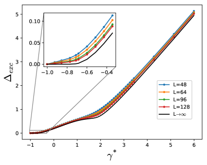
Figure 5: Spin excitation gap above the $S^{z}_{\rm total}=0$ ground state. In the inset one can see a gapless phase. DMRG results for finite chains of lengths $L=48,64,96,128$ and their $1/L$ extrapolations (black line) for a wide range $\gamma^{\ast}>-1$.

The computations were carried out for finite-length systems with $L=48,64,96$ and $128$ sites, using the ALPS library [ALPS_1, ; ALPS_2, ]. System parameters are set to $J=1$, $D_{0}=tan(\pi/6)$ and $D_{1}=0.2$, while the bare value of the anisotropy $\Delta$ is varied providing values of $-1<\gamma^{\ast}\leq 6$. This restricts the ground state analysis to the $S_{z}^{tot}=0$ subspace. Keeping m = 400 states and performing 10 sweeps we reproduced exact energies and expectation values at $\gamma^{\ast}=0$ for the same lengths with accuracy of at least 6 digits. Open boundary conditions on the alternating coupling have been chosen in a topologically trivial sector, so as to avoid gapless edge states. Averages of local expectation values are computed in the central half of each chain in order to minimize open boundary effects.

In Fig. 5 we show the excitation gap numerically computed as

$$\Delta_{exc}=E_{0}(N+1)+E(N+1)-2E(N)\,,$$ (75)

where $E_{0}(f)$ is the lowest energy state in the subspace with fermionic occupation number $f$ and $N=L/2$ corresponds to the $S_{z}^{tot}=0$ subspace. In the inset one can appreciate the gapless LL region described in subsection IV.2, in full agreement with bosonization predictions. It is also apparent the exponentially small gap opening at $\gamma^{\ast}_{c1}\sim 0.7$, supporting the presence of the BKT transition discussed in subsection IV.3. The gap value for $\gamma^{\ast}=0$ of course coincides with exact results in section II.

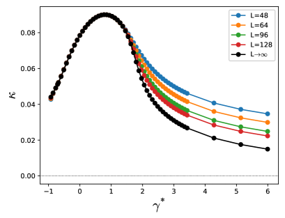
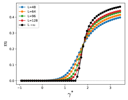
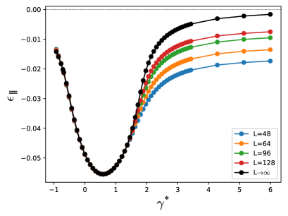
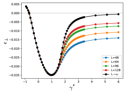
Figure 6: Various order parameters, computed as staggered averages of local ground state expectation values. Top right panel: spin chirality. Top left panel: staggered magnetization. Bottom panels: longitudinal and transverse spin-spin correlations. DMRG results for finite chains and their $1/L$ extrapolations.

In Fig. 6 we show the various order parameters discussed in the previous Sections. The top right panel shows the staggered part of the chirality operator expectation value in the ground state. These results confirm that the long-range spin chirality dimer order, already computed at $\gamma^{\ast}=0$ in section II, remains present for $\gamma^{\ast}>-1$ with a maximum at $\gamma^{\ast}\approx 1$. The top right panel shows the $z$-component of the staggered magnetization in the $S_{z}^{tot}=0$ ground state. One can see that it is strictly zero for $-1<\gamma^{\ast}<\gamma^{\ast}_{c2}\sim 2.5$ and raises suddenly thereof. This agrees with the bosonization analysis in subsection IV.4, signaling an Ising transition to the antiferromagnetic ordered phase. Finally, in the bottom panels we show the staggered part of the transverse and longitudinal components of the spin exchange. Oscillations of both components tend to zero as AFM LRO dominates and $|\langle S^{z}_{n}\rangle|$ tends to $0.5$.

VI Summary

In this paper, we have studied the ground-state properties of the one-dimensional spin $S=1/2$ XXZ Heisenberg chain with spatially modulated Dzyaloshinskii-Moriya (DM) interaction. Our goal was to describe the interplay between the uniform and staggered parts of the DM interaction which, when acting alone, do not change the excitation spectrum of the system. We have shown that joint effect of the uniform and staggered components of the DM coupling opens a possibility for formation of unconventional gapped phases in the ground-state of the system

Depending on the effective anisotropy parameter $\gamma^{\ast}=J_{z}/\sqrt{J^{2}+D_{0}^{2}+D_{1}^{2}}$, besides the standard ferromagnetic at $\gamma^{\ast}\leq-1$ and gapless Luttinger-liquid phase at $-1<\gamma^{\ast}<\gamma^{\ast}_{c1}$, the ground state phase diagram of the model contains two unconventional composite gapped phases. The gapped C1 phase exists for $\gamma^{\ast}_{c1}<\gamma^{\ast}<\gamma^{\ast}_{c2}$ and is characterized by the coexistence of LRO dimerization and alternating spin chirality patterns, while the composite C2 phase, which is realized at $\gamma^{\ast}>\gamma^{\ast}_{c2}>1$, is characterized by the presence, in addition to the dimerization and alternating spin chirality order, of long-range antiferromagnetic order.

Exploring the critical properties of the effective double sine-Gordon theory we argue, that the transition from the LL to the C1 phase at $\gamma^{\ast}_{c1}$ belongs to the Berezinskii-Kosterlitz-Thouless universality class, while the transition at $\gamma^{\ast}=\gamma^{\ast}_{c2}$ from C1 to C2 phase is of the Ising type. Extensive DMRG results support these statements.

VII Acknowledgment

We are grateful to A.A. Nersesyan and D.C. Cabra for their interest in this work and helpful comments.

References

• (1) H.-J. Mikeska and A. K. Kolezhuk, in Quantum Magnetism, edited by U. Schollwok et al. (Springer, Berlin, 2004).
• (2) C. Broholm et al., Magnetized States of Quantum Spin Chains in High Magnetic Fields, Lecture Notes in Physics 595, 211-234, (2008).
• (3) A. Vasiliev, O. Volkova, E. Zvereva, and M. Markina, Milestones of low-D quantum magnetism, npj Quantum Materials 18 (2018).
• (4) A.A. Zvyagin, Fiz. Niz. Temp. 15 977 (1989); A.A. Zvyagin, Zh. Eksp. Teor. Fiz. 98, 1396 (1990); F.C. Alkaraz and W.F. Wreszinski, J. Stat. Phys. 58 45-56 (1990). 131 H.-P. Eckle and C.J. Hamer, J. Phys. A: Math. Gen. 24 191 (1991). A.A. Zvyagin, J. Phys.: Cond. Matter. 3, 3865 (1991).
• (5) O.Derzhko, A.Moina Ferroelectrics 153, 49-54 (1994); O. Derzhko, J. Richter, and O. Zaburannyi, Jour. of Physics: Cond. Matt., 12, 8661 (2000); O. Derzhko, T. Verkholyak, T. Krokhmalskii, H. Büttner Phys. Rev. B 73, 214407 (2006); S. Roy, T. Chanda, T. Das, D. Sadhukhan, A. Sen(De), U. Sen, Phys. Rev. B 99 064422 (2019).
• (6) T. Verkholyak, O. Derzhko, T. Krokhmalskii, and J. Stolze, Phys. Rev. B 76, 144418 (2007).
• (7) M. Oshikawa and I. Affleck, Phys. Rev. Lett. 79, 2883 (1997). I. Affleck and M. Oshikawa, Phys. Rev. B 60 1038 (1999).
• (8) J. Z. Zhao, X. Q. Wang, T. Xiang, Z. B. Su, and L. Yu, Phys. Rev. Lett. 90, 207204 (2003).
• (9) S. Mahdavifar, M. R. Soltani, A. A. Masoudi, Eur. Phys. J. B 62, 215 (2008).
• (10) D. N. Aristov and S. V. Maleyev, Phys. Rev. B 62, R751 (2000).
• (11) M. Bocquet, F.H.L. Essler, A.M. Tsvelik, and A.O. Gogolin, Phys. Rev. B 64, 094425 (2001).
• (12) S. Gangadharaiah, J. Sun, and O. A. Starykh, Phys. Rev. B 78, 054436 (2008).
• (13) I. Garate and I. Affeck, Phys. Rev. B 81, 144419 (2010).
• (14) Yang-Hao Chan, Wen Jin, Hong-Chen Jiang, and O. A. Starykh, Phys. Rev. B 96 214441 (2017).
• (15) S. Peotta, L. Mazza, E. Vicari, M. Polini, R. Fazio, and D. Rossini, J. Stat. Mech. P09005 (2014).
• (16) Zhihao Hao, Yuan Wan, Ioannis Rousochatzakis, Julia Wildeboer, A. Seidel, F. Mila, and O. Tchernyshyov, Phys. Rev. B 84, 094452 (2011).
• (17) M. Kargarian, R. Jafari, A. Langari, Phys. Rev. A 79, 042319 (2009).
• (18) E. Mehran, S. Mahdavifar, R. Jafari, Phys. Rev. A 89, 049903, (2014).
• (19) R. Jafari, M. Kargarian, A. Langari, and M. Siahatgar Phys. Rev. B 78, 214414 (2008). M.R. Soltani, S. Mahdavifar, A. Akbari, A. A. Masoudi, Jour. of Superconductivity and Novel Magnetism, 23, 1369 (2010). M. R. Soltani, J. Vahedi, S. Mahdavifar, Physica A: Stat. Mechanics and its Applications, 416, 321 (2014). H. Cheraghi, S. Mahdavifar, Jour. of Phys.: Cond. Matt., 30, 42LT01, (2018).
• (20) J. Streska, L. Galisova and O. Strezhko, Acta Phys. Polonica 118, 742 (2010). Bo Li, Sam Young Cho, Hong-Lei Wang and Bing-Quan Hu, Jour.of Physics A: Math. Theor., 44, 392002 (2011). N. Amiri, A. Langari, Phys. Status Solidi B 250, 537 (2013).
• (21) I. E. Dzyaloshinskii, Sov. Phys. JETP, 5, 1259 (1957);
I. E. Dzyaloshinskii, J. Phys. Chem. Solids, 4, 241 (1958).
• (22) T. Moriya, Phys. Rev. Lett. 4, 288 (1960); T. Moriya, Phys. Rev. 120, 91 (1960).
• (23) I. E. Dzyaloshinskii, Zh. Eksp. Teor. Fiz. 46 1420 (1964); [Sov. Phys.-JETP 19 960(1964)]; I E. Dzyaloshinskii, Zh. Eksp. Teor. Fiz. 47, 992 (1964). [Sov. Phys. - JETP 20, 665 (1965).]
• (24) O.M. Volkov, D.D. Sheka, Y. Gaididei, V.P. Kravchuk, U.K. Rössler, J. Fassbender, and D. Makarov, Scientific Reports 8, Article number: 866 (2018).
• (25) H. Yang, O. Boulle, V. Cros, A. Fert, and M. Chshiev, Scientific Reports, 8, Article N: 12356 (2018).
• (26) W. Zhang, et al., App. Phys. Lett. 113, 122406 (2018).
• (27) T. Srivastava et al., Nano Lett. 18, 4871 (2018).
• (28) R. Ramesh and N. A. Spaldin, Nat. Mater. 6, 21 (2007); M. Bibes and A. Barthelemy, Nat. Mater. 7, 425 (2008).
• (29) H. Katsura, N. Nagaosa, and A. V. Balatsky, Phys. Rev. Lett. 95, 057205 (2005).
• (30) S.-W. Cheong and M. Mostovoy, Nature Materials 6, 13 (2007); M. Azimi, L. Chotorlishvili, S. K. Mishra, S. Greschner, T. Vekua, J. Berakdar, Phys. Rev. B 89, 024424 (2014); L. Chotorlishvili, R. Khomeriki, A. Sukhov, S. Ruffo, and J. Berakdar Phys. Rev. Lett. 111, 117202 (2013); M. Azimi, M. Sekania, S. K. Mishra, L. Chotorlishvili, Z. Toklikishvili, J.Berakdar, Phys. Rev. B 94, 064423 (2016).
• (31) P. Jordan and E. Wigner Z. Phys. 47 631 (1928).
• (32) M. Takahashi, Thermodynamics of One Dimensional Solv- able Models (Cambridge University Press, Cambridge, 1999).
• (33) A. V. Chubukov, Phys. Rev. B 44, 4693 (1991).
• (34) T. Hikihara, L. Kecke, T. Momoi and A. Furusaki, Phys. Rev. B 78 144404 (2008).
• (35) W. P. Su, J. R. Schrieffer, and A. J. Heeger. Phys. Rev. Lett. 42, 1698 (1979).
• (36) I. Affleck, in Champs, Cordes et Phénomènes Critiques/ Fields, strings and critical phenomena, Eds. E. Brézin and J. Zinn-Justin, Elsevier, Amsterdam, (1990).
• (37) A. O. Gogolin, A. A. Nersesyan and A. M. Tsvelik, Bosonization and strongly correlated systems, Cambridge University Press (1998).
• (38) T. Giamarchi, ”Quantum Physics in One Dimension” (Oxford University Press, Oxford, 2004).
• (39) T. Hikihara and A. Furusaki, Phys. Rev. B 58, R583 (1998).
• (40) S. Lukyanov, V. Terras, Nuclear Physics B 654, 323 (2003).
• (41) A. Luther and I. Peschel, Phys. Rev. B 12, 3908 (1975).
• (42) R.K. Boullough, P.J. Caudrey, and H.M Gibbs in Solitons Springer-Verlag 1980,pg 107-141.
• (43) G. Delfino and G. Mussardo, Nucl. Phys. B 516, 675 (1998).
• (44) M. Fabrizio, A. O. Gogolin, A. A. Nersesyan, Phys. Rev. Lett. 83 2014 (1999).
• (45) M. Fabrizio, A. O. Gogolin, A. A. Nersesyan, Nucl.Phys. B 580 647 (2000).
• (46) Z. Bajnok, L. Palla, G. Takacs, F. Wagner, Nucl. Phys. B 601 503, (2001).
• (47) G. Takacs and F. Wagner, Nucl. Phys. B 741, 353 (2006).
• (48) M. Tsuchiizu and E. Orignac, J. Phys. Chem. Solids 63, 1459 (2002).
• (49) H. Otsuka and M. Nakamura, Phys. Rev. B 70, 073105 (2004).
• (50) G. Mussardo, V. Riva, G. Sotkov, Nucl. Phys. B 687, 189 (2004).
• (51) G.I. Japaridze and A.A. Nersesyan, Phys. Rev. B 99, 035134 (2019).
• (52) J. M. Kosterlitz and D. J. Thouless, J. Phys. C 11, 1583 (1973).
• (53) A. Takhtadjan and L. D. Faddeev, Theor. Math. Phys. 25, 147 (1975).
• (54) Al. B. Zamolodchikov, Int. J. Mod. Phys. A 10, 1125 (1995).
• (55) K. A. Muttalib and V. J. Emery, Phys. Rev. Lett. 57, 1370 (1986); T. Giamarchi and H. J. Schulz, Jour. Phys. (Paris) 49, 819 (1988); Phys. Rev. B 33, 2066 (1986).
• (56) S. Lukyanov and A. Zamolodchikov, Nucl. Phys. B 493, 571 (1997).
• (57) S.R. White, Phys. Rev. Lett. 69, 2863 (1992).
• (58) A.F. Albuquerque et al. (ALPS collaboration), Journal of Magnetism and Magnetic Materials 310, 1187 (2007).
• (59) B. Bauer et al. (ALPS collaboration), Journal of Statistical Mechanics: Theory and Experiment 05, P05001 (2011).