A permutation-based Bayesian approach for inverse covariance estimation

Abstract

Covariance estimation and selection for multivariate datasets in a high-dimensional regime is a fundamental problem in modern statistics. Gaussian graphical models are a popular class of models used for this purpose. Current Bayesian methods for inverse covariance matrix estimation under Gaussian graphical models require the underlying graph and hence the ordering of variables to be known. However, in practice, such information on the true underlying model is often unavailable. We therefore propose a novel permutation-based Bayesian approach to tackle the unknown variable ordering issue. In particular, we utilize multiple maximum a posteriori estimates under the DAG-Wishart prior for each permutation, and subsequently construct the final estimate of the inverse covariance matrix. The proposed estimator has smaller variability and yields order-invariant property. We establish posterior convergence rates under mild assumptions and illustrate that our method outperforms existing approaches in estimating the inverse covariance matrices via simulation studies.

Keywords: Gaussian graphical model; inverse covariance matrix; posterior convergence rate; high-dimensional analysis.

1 Introduction

In modern day statistics, datasets where the number of variables is much larger than the number of samples are more pervasive than they have ever been. Especially in recent years, due to advances in science and technology, data from genomics, finance, environmental and marketing applications are being generated at a rapid pace. One of the major challenges in this setting is to formulate models and develop inferential procedures to understand the complex relationships and multivariate dependencies present in these datasets. In high-dimensional settings, the sample covariance matrix can perform rather poorly. To address the challenge posed by high-dimensionality, several promising methods have been proposed in the literature. In particular, methods inducing sparsity in the Cholesky factor of the inverse covariance matrix $\Omega$ have proven to be very effective in applications. The sparsity patterns in the Cholesky factor of $\Omega$ can be uniquely encoded in terms of appropriate graphs. Hence the corresponding models are often referred to as directed acyclic graph (DAG) models.

In this paper, we focus on Gaussian DAG models. In particular, suppose we have i.i.d. observations ${\bm{Y}}_{1},{\bm{Y}}_{2},\cdots,{\bm{Y}}_{n}$ from a $p$-variate normal distribution with mean vector ${\bf 0}$ and covariance matrix $\Sigma$. Let $\Omega=\Sigma^{-1}=LD^{-1}L^{T}$ be the modified Cholesky decomposition (MCD) of the inverse covariance matrix, i.e., $L$ is a lower triangular matrix with unit diagonal entries, and $D$ is a diagonal matrix with positive diagonal entries. For a DAG model, this normal distribution is assumed to be Markov with respect to a given directed acyclic graph $\mathcal{D}$ with vertices $\{1,2,\ldots,p\}$. This is equivalent to saying that $L_{ij}=0$ whenever $\mathcal{D}$ does not have a directed edge from $i$ to $j$ (these concepts are discussed in detail in Section 2).

There exist several approaches in the literature for estimation of $\Omega$ and the underling graph based on Gaussian DAG models. Rütimann and Bühlmann (2009) introduce a graph-based technique for estimating sparse covariance and inverse covariance matrices by first inferring the underlying DAG using the PC-algorithm in (Kalisch and Bühlmann, 2007), and estimating the DAG-based covariance matrix and its inverse via the MCD approach. The other type of methods are based on regularized likelihood/pseudolikelihood. Chang and Tsay (2010) propose a parsimonious approach to estimate high-dimensional covariance matrices via MCD using $\ell_{1}$ penalization. Similar approach has also been adopted in (Shojaie and Michailidis, 2010) via the general weighted lasso to estimate the adjacency matrix of DAGs with given ordering. The authors in (van de Geer and Bühlmann, 2013) show that the $\ell_{0}$-penalized maximum likelihood estimator of the Cholesky factor converges in Frobenius norm in high dimensions under unknown ordering.

On the Bayesian side, when the underlying graph is known, literature exists that explores the posterior convergence rates for Gaussian concentration graph models, which induce sparsity in the inverse covariance matrix $\Omega$. When the underlying graph is unknown and needs to be selected, comparatively fewer works have tackled with asymptotic properties. Recently, (Ben-David, Li, Massam, and Rajaratnam, 2016) introduce a flexible and general class of ‘DAG-Wishart’ priors with multiple shape parameters, which are adaptations/generalizations of the Wishart distribution in the DAG context. The authors in (Cao, Khare, and Ghosh, 2019) establish both strong model selection consistency (in the terminology of (Cao, Khare, and Ghosh, 2019)) and posterior convergence rates for sparse Gaussian DAG models with DAG-Wishart distributions in a high-dimensional regime. However, the known ordering for these variables is required in order to achieve consistency, which can be problematic in practice, especially when the nature ordering is not available or not per-determined in the format of location or time sequence.

Recently, (Kang and Deng, 2017) adopt an improved MCD approach to tackle the variable order issue in estimating sparse inverse covariance matrix and consider an ensemble estimate under multiple permutations of the variable orders in a frequentist framework, which inspires us to propose a Bayesian ensemble estimate for estimation of $\Omega$ with these DAG-Wishart priors. Specifically, we utilize the multiple MAP (maximum a posteriori) estimates of the Cholesky factor under each permutation, and subsequently construct the final estimate of the inverse covariance matrix. To further encourage the sparsity pattern in the estimate, we also adopt the hard thresholding technique also implemented in (Kang and Deng, 2017; Cao, Khare, and Ghosh, 2019) to obtain the final estimate. The proposed estimator has small variability and yields order-invariant property. Under mild assumptions, we establish much better posterior convergence rates under DAG-Wishart distributions.

The rest of the paper is structured as follows. Section 2 provides background material from graph theory and Gaussian DAG models. In Section 3 we present our proposed Bayesian approach for precision matrix estimation based on permutation and the posterior convergence rates are provided in Section 5. In Section 4 we use simulation experiments to illustrate the proposed method, and demonstrate the benefits of our Bayesian approach for inverse covariance matrix estimation vis-a-vis existing Bayesian and penalized likelihood approaches. We end our paper with a discussion session in Section 6.

2 Preliminaries

In this section, we provide the necessary background material from graph theory, Gaussian DAG models, and DAG-Wishart distributions.

2.1 Gaussian DAG models

Throughout this paper, a directed acyclic graph (DAG) $\mathcal{D}=(V,E)$ consists of the vertex set $V=\{1,\ldots,p\}$ and an edge set $E$ such that there is no directed path starting and ending at the same vertex. For any given parent ordering, where that all the edges are directed from larger vertices to smaller vertices, denote $pa_{i}(\mathcal{D})$ as the set of parents of $i$ to be the collection of all vertices which are larger than $i$ and share an edge with $i$. Similarly, for any given parent ordering, the set of children of $i$, denoted by $chi_{i}(\mathcal{D})$, is the collection of all vertices which are smaller than $i$ and share an edge with $i$.

A Gaussian DAG model over a given DAG $\mathcal{D}$, denoted by $\mathcal{N}_{\mathcal{D}}$, consists of all multivariate Gaussian distributions which obey the directed Markov property with respect to a DAG $\mathcal{D}$. In particular, if ${y}=(y_{1},\ldots,y_{p})^{T}\sim N_{p}(0,\Sigma)$ and $N_{p}(0,\Sigma)\in\mathcal{N}_{\mathcal{D}}$, then $y_{i}\perp{y}_{\{i+1,\ldots,p\}\backslash pa_{i}(\mathcal{D})}|{y}_{pa_{i}(\mathcal{D})}$ for each $i$.

Any positive definite matrix $\Omega$ can be uniquely decomposed as $\Omega=LD^{-1}L^{T}$, where $L$ is a lower triangular matrix with unit diagonal entries, and $D$ is a diagonal matrix with positive diagonal entries. This decomposition is known as the modified Cholesky decomposition of $\Omega$ (see for example Pourahmadi (2007)). It is well-known that if $\Omega=LD^{-1}L^{T}$ is the modified Cholesky decomposition of $\Omega$, then $N_{p}(0,\Omega^{-1})\in\mathcal{N}_{\mathcal{D}}$ if and only if $L_{ij}=0$ whenever $i\notin pa_{j}(\mathcal{D})$. In other words, the structure of the DAG $\mathcal{D}$ is reflected in the Cholesky factor of the inverse covariance matrix. In light of this, it is often more convenient to reparametrize in terms of the Cholesky parameter of the inverse covariance matrix as follows.

Given a DAG $\mathcal{D}$ on $p$ vertices, denote $\mathcal{L}_{\mathcal{D}}$ as the set of lower triangular matrices with unit diagonals and $L_{ij}=0$ if $i\notin pa_{j}(\mathcal{D})$, and let $\mathcal{D}_{+}^{p}$ be the set of strictly positive diagonal matrices in $\mathbb{R}^{p\times p}$. We refer to $\Theta_{\mathcal{D}}=\mathcal{D}_{+}^{p}\times\mathcal{L}_{\mathcal{D}}$ as the Cholesky space corresponding to $\mathcal{D}$, and $(D,L)\in\Theta_{\mathcal{D}}$ as the Cholesky parameter corresponding to $\mathcal{D}$. In fact, the relationship between the DAG and the Cholesky parameter implies that

$$\mathcal{N}_{\mathcal{D}}=\{N_{p}(0,(L^{T})^{-1}DL^{-1}):(D,L)\in\Theta_{\mathcal{D}}\}.$$

2.2 DAG-Wishart distribution

In this section, we specify the multiple shape parameter DAG-Wishart distributions introduced in Ben-David et al. (2016). First, we provide required notation on matrix. Given a directed graph $\mathcal{D}=(V,E)$, with $V=\{1,\ldots,q\}$, and a $q\times q$ matrix $A$, denote the column vectors $A_{\mathcal{D}.i}^{>}=(A_{ij})_{j\in pa_{i}(\mathcal{D})}$ and $A_{\mathcal{D}.i}^{\geq}=(A_{ii},(A_{\mathcal{D}.i}^{>})^{T})^{T}.$ Also, let $A_{\mathcal{D}}^{>i}=(A_{kj})_{k,j\in pa_{i}(\mathcal{D})}$,

$$A_{\mathcal{D}}^{\geq i}=\left[\begin{matrix}A_{ii}&(A_{\mathcal{D}.i}^{>})^{T}\\ A_{\mathcal{D}.i}^{>}&A_{\mathcal{D}}^{>i}\end{matrix}\right].$$

In particular, $A_{\mathcal{D}.q}^{\geq}=A_{\mathcal{D}}^{\geq q}=A_{qq}$.

The DAG-Wishart distributions in Ben-David et al. (2016) corresponding to a DAG $\mathcal{D}$ are defined on the Cholesky space $\Theta_{\mathcal{D}}$. Given a positive definite matrix $U$ and a $p$-dimensional vector ${\bm{\alpha}}(\mathcal{D})$, the (unnormalized) density of the DAG-Wishart distribution on $\Theta_{\mathcal{D}}$ is given by

$$\exp\{-\frac{1}{2}\mbox{tr}((LD^{-1}L^{T})U)\}\prod_{i=1}^{p}D_{ii}^{-\frac{\alpha_{i}(\mathcal{D})}{2}},$$ (1)

for every $(D,L)\in\Theta_{\mathcal{D}}$. Let $\nu_{i}(\mathcal{D})=|pa_{i}(\mathcal{D})|=|\{j:j>i,(j,i)\in E({\mathcal{D}})\}|$. If $\alpha_{i}(\mathcal{D})-\nu_{i}(\mathcal{D})>2$, for all $1\leq i\leq q$, the density in (1) can be normalized to a probability density, and the normalizing constant is given by

$$\gamma_{\mathcal{D}}(U,{\bm{\alpha}}(\mathcal{D}))=\prod_{i=1}^{q}\frac{\Gamma(\frac{\alpha_{i}(\mathcal{D})}{2}-\frac{\nu_{i}(\mathcal{D})}{2}-1)2^{\frac{\alpha_{i}(\mathcal{D})}{2}-1}(\sqrt{\pi})^{\nu_{i}(\mathcal{D})}det(U_{\mathcal{D}}^{>i})^{\frac{\alpha_{i}(\mathcal{D})}{2}-\frac{\nu_{i}(\mathcal{D})}{2}-\frac{3}{2}}}{det(U_{\mathcal{D}}^{\geq i})^{\frac{\alpha_{i}(\mathcal{D})}{2}-\frac{\nu_{i}(\mathcal{D})}{2}-1}},$$ (2)

In this case, we define the following DAG-Wishart density with $q$ shape parameters $\{\alpha_{i}(\mathcal{D})\}_{i=1}^{q}$ which can be used for differential shrinkage of the variables in high-dimensional settings, $\pi_{U,\alpha(\mathcal{D})}^{\Theta_{\mathcal{D}}}$ on the Cholesky space $\Theta_{\mathcal{D}}$ by

$$\pi_{U,\alpha(\mathcal{D})}^{\Theta_{\mathcal{D}}}(D,L)=\frac{1}{\gamma_{\mathcal{D}}(U,{\bm{\alpha}}(\mathcal{D}))}\exp\{-\frac{1}{2}\mbox{tr}((LD^{-1}L^{T})U)\}\prod_{i=1}^{q}D_{ii}^{-\frac{\alpha_{i}(\mathcal{D})}{2}}$$ (3)

for every $(D,L)\in\Theta_{\mathcal{D}}$.

The class of densities $\pi_{U,\alpha(\mathcal{D})}^{\Theta_{\mathcal{D}}}$ form a conjugate family of priors for the Gaussian DAG model $\mathcal{N}(\mathcal{D})$. In particular, as indicated in (Ben-David et al., 2016), we have the following result that gives the MAP (maximum a posteriori) estimate for our Cholesky parameter.

Proposition 2.1.

If the prior on $(D,L)\in\Theta_{\mathcal{D}}$ is $\pi_{U,\alpha(\mathcal{D})}^{\Theta_{\mathcal{D}}}$ and ${Y}_{1},\ldots,{Y}_{n}$ are independent, identically distributed $N_{p}({0},(L^{T})^{-1}DL^{-1})$ random vectors, then the posterior distribution of $(D,L)$ is $\pi_{\tilde{U},\tilde{\alpha}(\mathcal{D})}^{\Theta_{\mathcal{D}}}$ with posterior mode $(\hat{D},\hat{L})$ satisfying,

$$\hat{D}_{ii}=\frac{\tilde{U}_{i|pa_{i}(\mathcal{D})}}{\alpha_{i}+n},\quad\hat{L}_{\mathcal{D}.i}^{>}=-[\tilde{U}_{\mathcal{D}}^{>i}]^{-1}\tilde{U}_{\mathcal{D}.i}^{>},$$ (4)

where $S=\frac{1}{n}\sum_{i=1}^{n}{Y}_{i}{Y}_{i}^{T}$ denotes the sample covariance matrix, $\tilde{U}=U+nS$, $\tilde{U}_{i|pa_{i}(\mathcal{D})}=\tilde{U}_{ii}-(\tilde{U}_{\mathcal{D}\cdot i}^{>})^{T}(\tilde{U}_{\mathcal{D}}^{>i})^{-1}\tilde{U}_{\mathcal{D}\cdot i}^{>}$, and $\tilde{\alpha}(\mathcal{D})=(n+\alpha_{1}(\mathcal{D}),\ldots,n+\alpha_{p}(\mathcal{D}))$.

Therefore, for any given DAG, Proposition 2.1 yields the posterior mode for the Cholesky parameter and hence, the precision matrix $\Omega$. In particular, if the DAG imposed on the DAG-Wishart distribution is the true DAG, Section 5 provides the results for the posterior convergence rate.

3 Bayesian approach for precision matrix estimation

Let $\bm{Y}=\left({\bm{Y}}_{1},{\bm{Y}}_{2},\cdots,{\bm{Y}}_{n}\right)^{T}\in\mathbb{R}^{n\times p}$ be the observed data. The closed form for the posterior mode specified in (4) is convenient. However, it requires the underlying DAG and accordingly, the parent ordering to be given, which is rather problematic in real applications, especially the case when the ordering of variables and the conditional independence between variables are both unknown. We therefore propose a Bayesian approach to combine the graph selection procedures in (Cao et al., 2019) and permutations techniques in (Kang and Deng, 2017) to address this uncertainty of ordering issue and gain the flexibility to ensemble the multiple estimates for the Cholesky parameters for each ordering respectively.

First we define a mapping function

$$\sigma:\{1,2,\ldots,p\}\rightarrow\{1,2,\ldots,p\},$$ (5)

such that $(\sigma(1),\sigma(2),\ldots,\sigma(p))$ represents a new permutation of $(1,2,\ldots,p)$. Define the corresponding permutation matrix $P_{\sigma}$ as follows. For each column in $P_{\sigma}$, all the entries in the $j$th column are set at 0 except the entry at the $\sigma(j)$th row equals to 1. Denote the new data matrix after permutation as

$$\bm{Y}_{\sigma}=\bm{Y}P_{\sigma},$$

and let

$$S_{\sigma}=\frac{1}{n}\bm{Y}_{\sigma}^{T}\bm{Y}_{\sigma}$$

denote the new sample covariance matrix.

In order to obtain the DAG-constraint posterior mode for the precision matrix with respect to this new data matrix $\bm{Y}_{\sigma}$, we must first acquire an appropriate estimate for the underlying DAG. The idea of hard thresholding the Cholesky factor of the sample covariance matrix to estimate the DAG structure has been implemented in (Bickel and Levina, 2008a, b; Cao, Khare, and Ghosh, 2019). In particular, Cao, Khare, and Ghosh (2019) illustrate the graph selection consistency under the DAG-Wishart priors though the following procedure along with the justification of adopting this method.

Algorithm 1 (Estimate of the underlying DAG).

Generate graphs by thresholding the modified Cholesky factor of $(S_{\sigma}+0.1I)^{-1}$ to get a sequence of $3000$ additional graphs, and search around all the above graphs using Shotgun Stochastic Search to generate even more candidate graphs.

Random partition the original data set $\bm{Y}_{\sigma}$ of $n$ observations into $10$ equal sized subsets. Each time a single subset is excluded, and the remaining $9$ subsets are used as our new sample. Repeat Step 1 for each new sample.

Compute the log posterior probabilities for all cadidate graphs and select the graph $\hat{\mathcal{D}}$ with the highest probability.

Remark 1.

The numbers in Algorithm 1 such as the length of sequence and the number of subsets can be modified depending on computational resources. Note that in Steps 2 and 3, due to the conjugacy of the DAG-Wishart distribution, the (marginal) posterior DAG probabilities can be computed as

$$\pi({\mathcal{D}}|{Y})\propto\frac{\gamma_{\mathcal{D}}(U+nS_{\sigma},n+{\alpha}(\mathcal{D}))}{\gamma_{\mathcal{D}}(U,{\alpha}(\mathcal{D}))}.$$ (6)

Now that we have the estimated DAG $\hat{\mathcal{D}}$ for the new data matrix $\bm{Y}_{\sigma}$, the natural question arises as how to regenerate the modified Choleksy parameter and obtain the appropriate estimate for the true precision matrix. We therefore propose to use the MAP (maximum a posteriori) estimate given in Proposition 2.1 with the following algorithm under permutation $\sigma$.

Algorithm 2 (MAP estimate of $\Omega$).

For $i=1,2,\ldots,p$, compute $d_{i}=\frac{\tilde{U}_{i|pa_{i}(\hat{\mathcal{D}})}}{\alpha_{i}+n},l_{i}=-[\tilde{U}_{\hat{\mathcal{D}}}^{>i}]^{-1}\tilde{U}_{\hat{\mathcal{D}}.i}^{>}$, where $\tilde{U}=nS_{\sigma}+U$. Set $d_{i}=0$ and $l_{i}=0$, whenever $pa_{i}(\hat{\mathcal{D}})=0$.

Reconstruct Cholesky parameter $(\hat{D}_{\sigma},\hat{L}_{\sigma})\in\Theta_{\hat{\mathcal{D}}}$ satisfying $\left(\hat{L}_{\sigma}\right)_{\hat{\mathcal{D}}.i}^{>}=l_{i}$ and $\hat{D}_{\sigma}=\mbox{diag}\left\{d_{1},d_{2},\ldots,d_{p}\right\}$.

Set $\hat{\Omega}_{\sigma}=\hat{L}_{\sigma}\hat{D}_{\sigma}^{-1}\hat{L}_{\sigma}^{T}$.

By transforming $\hat{D}_{\sigma}$, $\hat{L}_{\sigma}$ and $\hat{\Omega}_{\sigma}$ to the original order, we can thereby estimate $D,L$ and $\Omega$ with

$$\hat{L}=P_{\sigma}\hat{L}_{\sigma}P_{\sigma}^{T},\quad\hat{D}=P_{\sigma}\hat{D}_{\sigma}P_{\sigma}^{T}$$ (7)

and

$$\hat{\Omega}=\hat{L}\hat{D}^{-1}\hat{L}^{T}=P_{\sigma}\hat{L}_{\sigma}P_{\sigma}^{T}(P_{\sigma}\hat{D}_{\sigma}P_{\sigma}^{T})^{-1}P_{\sigma}\hat{L}_{\sigma}^{T}P_{\sigma}^{T}=P_{\sigma}\hat{\Omega}_{\sigma}P_{\sigma}^{T}.$$ (8)

Now suppose we generate $K$ permutations denoted as $\sigma_{1},\sigma_{2},\ldots,\sigma_{K}$. For each permutation $\sigma_{k}$ $(1\leq k\leq K)$, Algorithm 2, (7) and (8) yield the corresponding estimates $\hat{L}_{k}$, $\hat{D}_{k}$ and $\hat{\Omega}_{k}$. Naturally, there are two ways for integrating these estimates. The first approach is to average $\Omega_{1},\Omega_{2},\ldots,\Omega_{K}$ and let $\bar{\Omega}=\frac{1}{K}\sum_{k=1}^{K}\hat{\Omega}_{k}$ be our final estimate for the true precision matrix. However, this average estimate performs poorly, as the estimation error of each $\hat{\Omega}_{k}$ is already aggregated by the error in both $\hat{L}_{k}$ and $\hat{D}_{k}$. We therefore propose to use the average estimates of both $\hat{L}_{k}$’s and $\hat{D}_{k}$’s to construct the ensemble estimate for $\Omega$. In particular, denote

$$\bar{L}=\frac{1}{K}\sum_{k=1}^{K}\hat{L}_{k},\quad\bar{D}=\frac{1}{K}\sum_{k=1}^{K}\hat{D}_{k},$$ (9)

and estimate $\Omega$ with

$$\check{\Omega}=\bar{L}\bar{D}^{-1}\bar{L}^{T}.$$ (10)

In Section 4, we will see this estimate can have the advantage of averaging the variability and better recover the individual entry values of the true precision matrix.

However, $\check{\Omega}$ does not necessarily carry out the true sparse pattern encoded in possibly very parse true inverse covariance matrix. Hence, we utilize the following hard thresholding procedure to encourage the sparsity in $\check{\Omega}$. For any given thresholding value $\tau$, construct the corresponding sparse matrix $\bar{L}_{\tau}$ based on $\bar{L}$ in (9) as follows. For $1\leq i,j\leq p$,

$$(\bar{L}_{\tau})_{ij}=\begin{cases}\bar{L}_{ij},&|\bar{L}_{ij}|>\tau\\ 0,&|\bar{L}_{ij}|\leq\tau.\end{cases}$$

Estimate $\Omega$ with $\check{\Omega}_{\tau}=\bar{L}_{\tau}\bar{D}^{-1}\bar{L}_{\tau}^{T}$. If we vary the thresholding value $\tau$ on a grid, the best thresholding value $\tau_{b}$ is selected, which minimizes the “BIC”-like measure defined as

$$BIC(\tau)=ntr(S\check{\Omega}_{\tau})-n\log|\check{\Omega}_{\tau}|+\log n*E,$$ (11)

where $E$ denotes the total numbers of non-zero entries in $\bar{L}_{\tau}$ and $\check{\Omega}_{\tau}=\bar{L}_{\tau}\bar{D}^{-1}\bar{L}_{\tau}^{T}.$ See examples in (Cao et al., 2019; Khare et al., 2017; Shojaie and Michailidis, 2010; Kang and Deng, 2017) for justifications of the “BIC-like criterion. Note that the estimate $\check{\Omega}_{\tau_{b}}$ possesses a much more sparse structure compared to $\check{\Omega}$ in (10) via the thresholding step, and could possibly better reveal the true sparsity pattern in the underlying precision matrix. Now we are ready to present the following algorithm for our proposed Bayesian approach for estimating precision matrix.

Algorithm 3.

Generate $K$ permutations $\sigma_{1},\sigma_{2},\ldots,\sigma_{K}$ and obtain the corresponding data matrix and sample covariance matrix $\bm{Y}_{\sigma_{k}}$, $S_{\sigma_{k}}$. For $1\leq k\leq K$, do step 1-3.

Implement Algorithm 1 and obtain the estimated DAG $\mathcal{D}_{\sigma_{k}}.$

Given $\mathcal{D}_{\sigma_{k}}$, obtain $\hat{L}_{\sigma_{k}}$, $\hat{D}_{\sigma_{k}}$, $\hat{\Omega}_{\sigma_{k}}$ via Algorithm 2.

Set $\hat{L}_{k}=P_{\sigma_{k}}\hat{L}_{\sigma_{k}}P_{\sigma_{k}}^{T},\quad\hat{D}_{k}=P_{\sigma_{k}}\hat{D}_{\sigma_{k}}P_{\sigma_{k}}^{T}$.

Obtain the average estimates $\bar{L}=\frac{1}{K}\sum_{k=1}^{K}\hat{L}_{k},\bar{D}=\frac{1}{K}\sum_{k=1}^{K}\hat{D}_{k},$ and $\check{\Omega}=\bar{L}\bar{D}^{-1}\bar{L}^{T}.$

Vary the thresholding values on a grid and select $\bar{L}_{\tau_{b}}$ according to the measure in (11).

Set $\check{\Omega}_{\tau_{b}}=\bar{L}_{\tau_{b}}\bar{D}^{-1}\bar{L}_{\tau_{b}}^{T}$ as the estimate for $\Omega$.

Remark 2.

We would like to point out that the hard thresholding procedure in Step 3 and 4 is not necessarily required, if one is merely interested in the estimation rather than the sparsity recovery of the precision matrix. As we will see in Section 4, no significant difference is observed in performance between the estimate $\check{\Omega}$ obtained in Step 4 and the final estimate $\check{\Omega}_{\tau_{b}}$ under certain settings. Hence, $\check{\Omega}$ can also serve as an alternate estimate in practice.

4 Simulation studies

In this section, we illustrate the potential advantage of utilizing the proposed Bayesian approach through simulation studies. We fix our number of observations $n=100$. We then consider different combinations of $(n,p)$ with $p$ ranging from smaller than $30$ to $200$, such that $p$ varies from smaller than $n$ to larger than $n$. Next, for each fixed $p$, a $p\times p$ positive definite matrix $\Omega_{0}$ is constructed. In particular, we consider the following five cases of $\Omega_{0}$, which are also considered in (Kang and Deng, 2017).

$Case\mbox{ }1$:

$\Omega_{0}$ has a banded structure such that the main diagonal entries equal to 1, while the first sub-diagonal entries equal to 0.5 and second sub-diagonals 0.3.

$Case\mbox{ }2$:

$\Sigma_{0}=\Omega_{0}^{-1}$ is autoregressive correlated such that $(\Sigma_{0})_{ij}=0.5^{|i-j|},$ for all $1\leq i\leq j\leq p$.

$Case\mbox{ }3$:

$\Omega_{0}$ has $3\%$ sparsity. For each fixed $p$, we start from a $p\times p$ identity matrix. Then, we randomly choose $3\%$ of the lower triangular entries and set the values to be randomly drawn from $\mbox{Unif}(0,1)$. We refer to this matrix as our true Cholesky factor $L_{0}$ and set $\Omega_{0}=L_{0}L_{0}^{T}$.

$Case\mbox{ }4$:

$\Omega_{0}$ has a $10\times 10$ compound structure matrix on the left top with diagonal elements 1 and others 0.5. Other entries of $\Omega_{0}$ are set to be zero, except for all the diagonals taken to be 1.

$Case\mbox{ }5$:

$\Omega_{0}$ is generated by randomly permuting rows and corresponding columns of the precision matrix in Case 4.

Next, for every case of $\Omega_{0}$, we generate $n$ i.i.d. observations from the $N(0_{p},\Omega_{0})$ distribution. We then estimate the true precision matrix $\Omega_{0}$ using both Bayesian and frequentist procedures outlined below.

$DAGW.BIC$:

Set the hyperparameters for our DAG-Wishart distribution in (3) as $U=I_{p}$, $\alpha_{i}(\mathcal{D})=\nu_{i}(\mathcal{D})+10$ for $i=1,2,\ldots,p$, and the total number of permutations $K=100$. Obtain our estimate $\check{\Omega}_{\tau_{b}}$ via Algorithm 3.

$DAGW$:

Under the same hyperparameter setting, obtain the estimate $\check{\Omega}$ via Algorithm 3, but without the step of hard thresholding, i.e., ${\tau_{b}}=0$.

$MLE$:

For each permutation, replace MAP in 2 with the $\mathcal{D}_{\sigma_{k}}$-constrained maximum likelihood estimate. Then implement step 2–4 in Algorithm 3 to obtain the ensemble MLE estimate.

$BAYES$:

Under the same hyperparameter setting, implement Algorithm 1 and 2 with the original data without permutations.

$MCD.BIC$:

Implement the improved MCD approach based on penalized likelihood approaches in (Kang and Deng, 2017) with BIC-based tuning.

$PC-DAG$:

Implement the PC-algorithm based approach for inverse covariance estimation introduced in (Rütimann and Bühlmann, 2009) encoded in R package “pcalg” with suggested tuning parameters.

We then compare the estimation performance between these six methods under the following five different losses. Stein’s loss is a commonly used loss function given by

$$L_{1}(\hat{\Omega},\Omega_{0})=tr(\hat{\Omega}\Omega_{0}^{-1})-\log(det(\Omega_{0}\Omega_{0}^{-1}))-p,$$

where $\hat{\Omega}$ represents the estimator of the true precision matrix $\Omega_{0}$. The modified mean absolute error loss and mean squared error loss, restricted to the functionally independent elements of the true precision matrix are defined as,

$$L_{2}(\hat{\Omega},\Omega_{0})=\sum_{i=1}^{q}\sum_{j\in pa_{i}(\mathcal{D}_{0})}\lvert(\Omega_{0})_{ji}-\hat{\Omega}_{ji}\rvert,\quad L_{3}(\hat{\Omega},\Omega_{0})=\sum_{i=1}^{q}\sum_{j\in pa_{i}(\mathcal{D}_{0})}\left((\Omega_{0})_{ji}-\hat{\Omega}_{ji}\right)^{2},$$

where $\mathcal{D}_{0}$ represents the true underlying DAG implying the sparsity pattern in $\Omega_{0}$. We also adopt the following two measures of accuracy: the general mean absolute error and mean squared error given by

$$L_{4}(\hat{\Omega},\Omega_{0})=\sum_{i=1}^{q}\sum_{j=1}^{q}\lvert(\Omega_{0})_{ji}-\hat{\Omega}_{ji}\rvert,\quad L_{5}(\hat{\Omega},\Omega_{0})=\sum_{i=1}^{q}\sum_{j=1}^{q}\left((\Omega_{0})_{ji}-\hat{\Omega}_{ji}\right)^{2}.$$

The summary of our results are presented in Table 1 to Table 5 corresponding to five different structures of the true precision matrix respectively. The five losses for six methods averaged over 20 repetitions and their corresponding standard errors (in parenthesis) for different approaches are shown in the tables. For each loss, the lowest averages among all the methods are highlighted. We can see from the results, under different scenarios of the true precision matrix, our proposed method DAGW.BIC and DAGW outperform other frequentist methods and Bayesian methods under almost all the five measures. In particular, when the dimension $p$ increases, our proposed permutation method with DAG-Wishart prior can sustain the higher dimension and achieve much better and more stable estimation results.

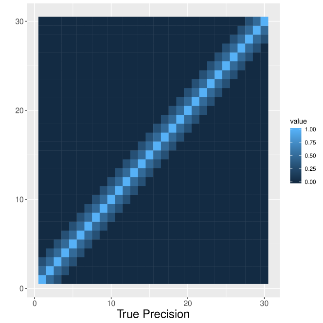
(a) True precision

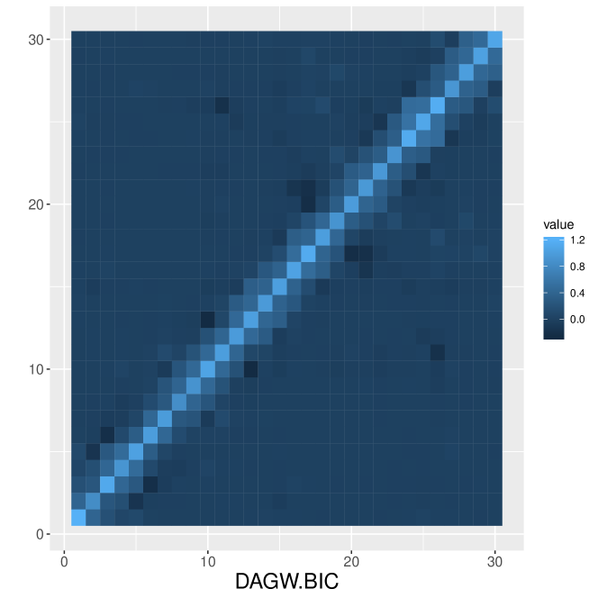
(b) DAGW.BIC

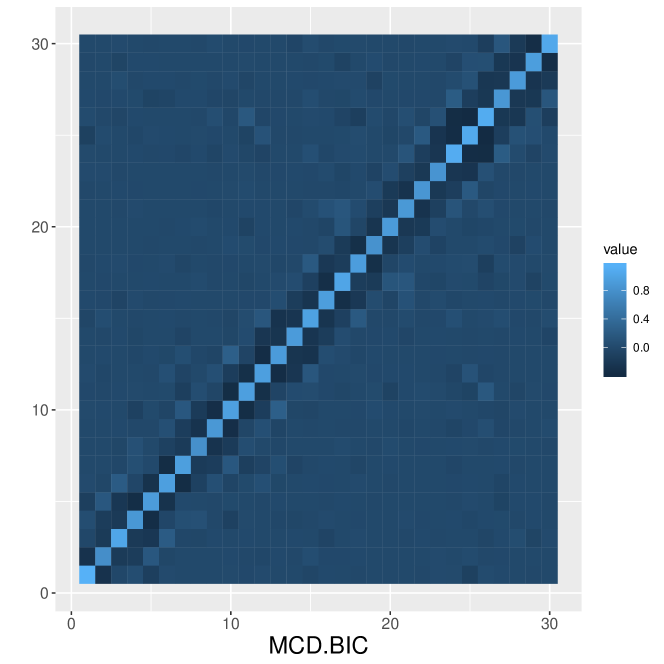
(c) MCD.BIC

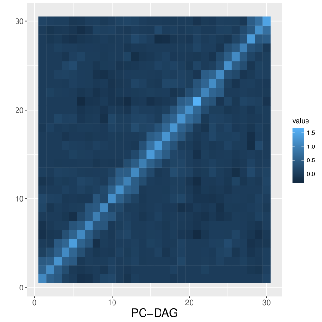
(d) PC-DAG

Figure 1: Heatmap comparison of estimates when $p=30$

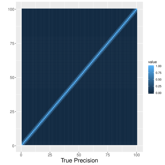
(a) True precision

(b) DAGW.BIC

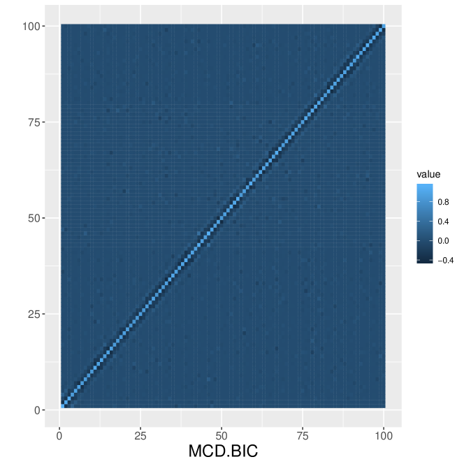
(c) MCD.BIC

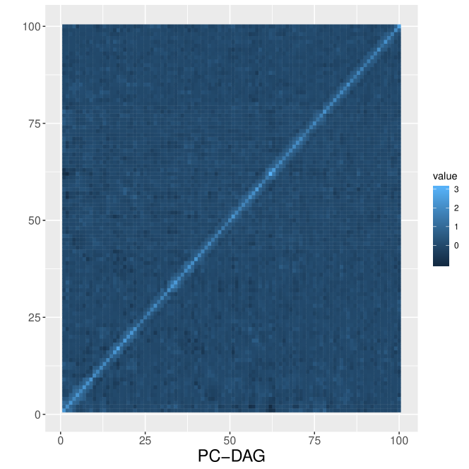
(d) PC-DAG

Figure 3: Heatmap comparison of estimates when $p=100$

To better visualize the simulation results, we plot the heatmap comparison between the true precision matrix and different estimators under different values of $p$ when the true precision matrix has a banded structure. In Figure 1 to Figure 3, we can see among all three estimators, our proposed method can best recover the sparse structure of the true precision matrix. MCD method in (Kang and Deng, 2017) fails to capture the structure for the first and second sub-diagonal entries, while the PC-DAG generates more false positives and obscures the true clear sparsity pattern.

		DAGW.BIC	DAGW	MLE	BAYES	MCD.BIC	PC-DAG
$p=30$	$L_{1}$	0.07 (0.01)	0.15 (0.01)	0.16 (0.01)	0.33 (0.00)	1.41 (0.05)	0.18 (0.02)
	$L_{2}$	0.03 (0.01)	0.03 (0.01)	0.04 (0.01)	0.32 (0.00)	0.80 (0.02)	0.10 (0.01)
	$L_{3}$	0.18 (0.02)	0.19 (0.02)	0.22 (0.02)	0.76 (0.00)	1.21 (0.02)	0.38 (0.03)
	$L_{4}$	0.08 (0.01)	0.19 (0.02)	0.24 (0.02)	0.88 (0.01)	1.67 (0.04)	0.29 (0.03)
	$L_{5}$	0.75 (0.06)	1.11 (0.07)	1.23 (0.08)	2.00 (0.01)	3.07 (0.06)	1.29 (0.11)
$p=50$	$L_{1}$	0.09 (0.01)	0.16 (0.01)	0.18 (0.01)	0.33 (0.00)	1.40 (0.03)	0.20 (0.02)
	$L_{2}$	0.03 (0.00)	0.03 (0.00)	0.03 (0.00)	0.33 (0.00)	0.78 (0.01)	0.11 (0.01)
	$L_{3}$	0.18 (0.01)	0.18 (0.01)	0.21 (0.01)	0.78 (0.00)	1.18 (0.01)	0.39 (0.03)
	$L_{4}$	0.10 (0.01)	0.20 (0.01)	0.25 (0.01)	0.90 (0.01)	1.64 (0.03)	0.31 (0.04)
	$L_{5}$	1.00 (0.06)	1.38 (0.05)	1.54 (0.06)	2.04 (0.01)	3.23 (0.08)	1.49 (0.11)
$p=100$	$L_{1}$	0.15 (0.01)	0.20 (0.01)	0.23 (0.01)	0.34 (0.00)	1.33 (0.02)	0.27 (0.01)
	$L_{2}$	0.03 (0.00)	0.03 (0.00)	0.04 (0.00)	0.33 (0.00)	0.75 (0.01)	0.11 (0.01)
	$L_{3}$	0.20 (0.01)	0.19 (0.01)	0.21 (0.01)	0.79 (0.00)	1.16 (0.01)	0.40 (0.02)
	$L_{4}$	0.16 (0.01)	0.22 (0.01)	0.29 (0.01)	0.91 (0.01)	1.55 (0.02)	0.36 (0.02)
	$L_{5}$	1.83 (0.08)	2.11 (0.07)	2.40 (0.08)	2.06 (0.01)	3.40 (0.08)	1.87 (0.07)
$p=150$	$L_{1}$	0.19 (0.01)	0.23 (0.01)	0.27 (0.01)	0.34 (0.02)	1.28 (0.02)	0.31 (0.01)
	$L_{2}$	0.05 (0.01)	0.04 (0.01)	0.04 (0.00)	0.34 (0.00)	0.71 (0.01)	0.12 (0.01)
	$L_{3}$	0.25 (0.02)	0.23 (0.01)	0.30 (0.01)	0.79 (0.00)	1.12 (0.02)	0.42 (0.02)
	$L_{4}$	0.19 (0.01)	0.23 (0.01)	0.30 (0.01)	0.92 (0.01)	1.51 (0.01)	0.40 (0.02)
	$L_{5}$	2.19 (0.05)	2.43 (0.05)	2.75 (0.05)	2.07 (0.01)	3.47 (0.03)	2.12 (0.07)
$p=200$	$L_{1}$	0.22 (0.01)	0.31 (0.01)	0.36 (0.01)	0.34 (0.00)	1.28 (0.03)	0.35 (0.01)
	$L_{2}$	0.08 (0.01)	0.07 (0.01)	0.06 (0.00)	0.34 (0.01)	0.71 (0.01)	0.12 (0.01)
	$L_{3}$	0.34 (0.01)	0.30 (0.01)	0.30 (0.01)	0.79 (0.02)	1.16 (0.02)	0.43 (0.02)
	$L_{4}$	0.22 (0.01)	0.26 (0.01)	0.32 (0.01)	0.92 (0.01)	1.48 (0.03)	0.44 (0.02)
	$L_{5}$	2.24 (0.01)	2.60 (0.02)	2.87 (0.03)	2.28 (0.01)	3.84 (0.11)	2.39 (0.06)

Table 1: The loss averages and standard errors (in parenthesis) of estimates when $\Omega_{0}$ has a banded structure.

		DAGW.BIC	DAGW	MLE	BAYES	MCD.BIC	PC-DAG
p=30	$L_{1}$	0.05 (0.01)	0.14 (0.01)	0.14 (0.01)	0.29 (0.00)	0.88 (0.03)	0.06 (0.01)
	$L_{2}$	0.05 (0.01)	0.11 (0.01)	0.10 (0.01)	0.43 (0.00)	1.15 (0.05)	0.04 (0.01)
	$L_{3}$	0.19 (0.02)	0.32 (0.01)	0.31 (0.01)	0.64 (0.00)	1.04 (0.02)	0.13 (0.03)
	$L_{4}$	0.26 (0.03)	0.76 (0.03)	0.73 (0.03)	1.28 (0.03)	2.43 (0.08)	0.26 (0.05)
	$L_{5}$	1.04 (0.05)	1.58 (0.04)	1.56 (0.04)	1.92 (0.03)	3.11 (0.10)	1.04 (0.12)
p=50	$L_{1}$	0.05 (0.00)	0.15 (0.01)	0.15 (0.01)	0.29 (0.00)	0.91 (0.04)	0.08 (0.01)
	$L_{2}$	0.05 (0.01)	0.11 (0.00)	0.11 (0.00)	0.44 (0.00)	1.12 (0.04)	0.07 (0.01)
	$L_{3}$	0.18 (0.01)	0.32 (0.01)	0.31 (0.01)	0.65 (0.00)	1.04 (0.02)	0.14 (0.01)
	$L_{4}$	0.26 (0.02)	0.79 (0.02)	0.76 (0.02)	1.31 (0.03)	2.49 (0.09)	0.37 (0.06)
	$L_{5}$	1.24 (0.04)	1.77 (0.04)	1.75 (0.04)	1.95 (0.03)	3.25 (0.17)	1.44 (0.13)
p=100	$L_{1}$	0.06 (0.00)	0.18 (0.01)	0.17 (0.02)	0.29 (0.01)	0.85 (0.02)	0.13 (0.01)
	$L_{2}$	0.05 (0.01)	0.13 (0.01)	0.12 (0.01)	0.44 (0.01)	1.10 (0.02)	0.08 (0.01)
	$L_{3}$	0.18 (0.01)	0.34 (0.01)	0.33 (0.01)	0.66 (0.02)	1.04 (0.01)	0.21 (0.01)
	$L_{4}$	0.27 (0.02)	0.87 (0.01)	0.82 (0.01)	1.33 (0.01)	2.39 (0.05)	0.59 (0.07)
	$L_{5}$	1.67 (0.05)	2.13 (0.03)	2.12 (0.03)	1.97 (0.01)	3.38 (0.06)	2.19 (0.15)
p=150	$L_{1}$	0.07 (0.00)	0.18 (0.01)	0.18 (0.01)	0.30 (0.00)	0.86 (0.02)	0.17 (0.01)
	$L_{2}$	0.06 (0.01)	0.14 (0.01)	0.13 (0.01)	0.44 (0.00)	1.10 (0.02)	0.14 (0.01)
	$L_{3}$	0.20 (0.01)	0.36 (0.01)	0.35 (0.01)	0.66 (0.01)	1.04 (0.01)	0.23 (0.01)
	$L_{4}$	0.29 (0.02)	0.91 (0.02)	0.86 (0.02)	1.32 (0.02)	2.41 (0.04)	0.85 (0.06)
	$L_{5}$	1.81 (0.05)	2.23 (0.03)	2.23 (0.03)	1.97 (0.02)	3.54 (0.13)	2.98 (0.19)
p=200	$L_{1}$	0.07 (0.00)	0.17 (0.01)	0.17 (0.00)	0.30 (0.01)	0.83 (0.02)	0.22 (0.01)
	$L_{2}$	0.08 (0.01)	0.15 (0.01)	0.14 (0.01)	0.44 (0.00)	1.07 (0.02)	0.16 (0.01)
	$L_{3}$	0.24 (0.01)	0.37 (0.01)	0.36 (0.01)	0.66 (0.01)	1.02 (0.02)	0.18 (0.01)
	$L_{4}$	0.33 (0.02)	0.92 (0.02)	0.86 (0.02)	1.33 (0.02)	2.39 (0.06)	1.08 (0.08)
	$L_{5}$	1.82 (0.03)	2.21 (0.02)	2.21 (0.02)	1.98 (0.02)	3.72 (0.07)	3.72 (0.17)

Table 2: The loss averages and standard errors (in parenthesis) of estimates when $\Omega_{0}$ is autoregressive.

		DAGW.BIC	DAGW	MLE	BAYES	MCD.BIC	PC-DAG
p=30	$L_{1}$	0.01 (0.00)	0.01 (0.01)	0.02 (0.00)	0.02 (0.00)	0.25 (0.01)	0.10 (0.01)
	$L_{2}$	0.01 (0.00)	0.01 (0.00)	0.01 (0.00)	0.01 (0.00)	0.25 (0.01)	0.01 (0.00)
	$L_{3}$	0.06 (0.01)	0.06 (0.02)	0.06 (0.02)	0.06 (0.01)	0.25 (0.01)	0.05 (0.01)
	$L_{4}$	0.03 (0.00)	0.03 (0.01)	0.03 (0.00)	0.05 (0.02)	0.55 (0.02)	0.27 (0.04)
	$L_{5}$	0.19 (0.01)	0.18 (0.01)	0.19 (0.01)	0.24 (0.01)	0.88 (0.07)	1.27 (0.11)
p=50	$L_{1}$	0.02 (0.00)	0.03 (0.02)	0.03 (0.00)	0.03 (0.00)	0.81 (0.02)	0.15 (0.01)
	$L_{2}$	0.02 (0.00)	0.02 (0.01)	0.02 (0.00)	0.02 (0.00)	0.79 (0.02)	0.02 (0.00)
	$L_{3}$	0.11 (0.00)	0.11 (0.01)	0.11 (0.00)	0.11 (0.01)	0.67 (0.01)	0.12 (0.01)
	$L_{4}$	0.05 (0.00)	0.05 (0.01)	0.05 (0.01)	0.07 (0.00)	1.71 (0.03)	0.43 (0.05)
	$L_{5}$	0.29 (0.01)	0.29 (0.03)	0.30 (0.01)	0.35 (0.01)	2.02 (0.07)	1.83 (0.11)
p=100	$L_{1}$	0.05 (0.01)	0.05 (0.01)	0.05 (0.01)	0.06 (0.00)	1.61 (0.03)	0.21 (0.01)
	$L_{2}$	0.05 (0.01)	0.05 (0.00)	0.05 (0.01)	0.05 (0.01)	1.27 (0.02)	0.04 (0.00)
	$L_{3}$	0.23 (0.00)	0.26 (0.01)	0.26 (0.00)	0.26 (0.01)	1.41 (0.01)	0.23 (0.01)
	$L_{4}$	0.10 (0.00)	0.11 (0.00)	0.11 (0.00)	0.13 (0.01)	2.83 (0.03)	0.65 (0.05)
	$L_{5}$	0.61 (0.01)	0.6 (0.01)	0.61 (0.00)	0.67 (0.01)	4.13 (0.09)	2.68 (0.10)
p=150	$L_{1}$	0.06 (0.00)	0.07 (0.01)	0.07 (0.00)	0.07 (0.00)	3.46 (0.09)	0.26 (0.01)
	$L_{2}$	0.06 (0.00)	0.06 (0.01)	0.07 (0.01)	0.07 (0.00)	2.30 (0.02)	0.06 (0.00)
	$L_{3}$	0.39 (0.00)	0.39 (0.01)	0.39 (0.03)	0.39 (0.01)	2.57 (0.01)	0.39 (0.01)
	$L_{4}$	0.15 (0.01)	0.14 (0.00)	0.15 (0.00)	0.17 (0.01)	5.37 (0.02)	0.80 (0.06)
	$L_{5}$	0.88 (0.01)	0.87 (0.01)	0.88 (0.01)	0.94 (0.00)	7.69 (0.12)	3.30 (0.15)
p=200	$L_{1}$	0.10 (0.00)	0.12 (0.00)	0.12 (0.01)	0.11 (0.00)	5.16 (0.12)	0.29 (0.01)
	$L_{2}$	0.10 (0.00)	0.10 (0.00)	0.11 (0.00)	0.11 (0.00)	3.06 (0.02)	0.12 (0.01)
	$L_{3}$	0.62 (0.00)	0.62 (0.01)	0.63 (0.00)	0.63 (0.00)	3.73 (0.01)	0.62 (0.02)
	$L_{4}$	0.23 (0.00)	0.23 (0.00)	0.23 (0.00)	0.26 (0.01)	7.38 (0.04)	0.86 (0.04)
	$L_{5}$	1.39 (0.01)	1.36 (0.01)	1.37 (0.00)	1.45 (0.01)	10.75 (0.08)	3.79 (0.10)

Table 3: The loss averages and standard errors (in parenthesis) of estimates when $\Omega_{0}$ has $3\%$ sparsity.

		DAGW.BIC	DAGW	MLE	BAYES	MCD.BIC	PC-DAG
p=30	$L_{1}$	0.06 (0.01)	0.20 (0.01)	0.16 (0.02)	0.08 (0.01)	0.21 (0.03)	0.13 (0.01)
	$L_{2}$	0.34 (0.01)	0.32 (0.02)	0.34 (0.04)	0.33 (0.01)	0.50 (0.02)	0.32 (0.01)
	$L_{3}$	0.72 (0.01)	0.69 (0.02)	0.71 (0.06)	0.70 (0.01)	0.86 (0.02)	0.70 (0.02)
	$L_{4}$	0.71 (0.02)	0.68 (0.03)	0.85 (0.08)	0.74 (0.03)	1.04 (0.04)	0.81 (0.03)
	$L_{5}$	1.54 (0.02)	1.52 (0.03)	1.78 (0.12)	1.66 (0.06)	2.19 (0.04)	2.17 (0.05)
p=50	$L_{1}$	0.01 (0.00)	0.04 (0.00)	0.04 (0.00)	0.02 (0.00)	0.03 (0.00)	0.25 (0.01)
	$L_{2}$	0.05 (0.00)	0.06 (0.00)	0.05 (0.00)	0.05 (0.00)	0.06 (0.00)	0.05 (0.00)
	$L_{3}$	0.11 (0.00)	0.11 (0.00)	0.11 (0.00)	0.11 (0.00)	0.11 (0.00)	0.11 (0.00)
	$L_{4}$	0.12 (0.00)	0.12 (0.00)	0.12 (0.00)	0.15 (0.01)	0.16 (0.01)	0.90 (0.05)
	$L_{5}$	0.30 (0.00)	0.31 (0.01)	0.44 (0.02)	0.38 (0.02)	0.87 (0.10)	2.89 (0.10)
p=100	$L_{1}$	0.02 (0.00)	0.07 (0.00)	0.07 (0.00)	0.04 (0.00)	0.04 (0.01)	0.18 (0.01)
	$L_{2}$	0.11 (0.00)	0.11 (0.00)	0.09 (0.01)	0.10 (0.00)	0.12 (0.00)	0.10 (0.00)
	$L_{3}$	0.22 (0.00)	0.22 (0.00)	0.23 (0.01)	0.22 (0.00)	0.23 (0.00)	0.24 (0.00)
	$L_{4}$	0.23 (0.00)	0.23 (0.01)	0.23 (0.02)	0.26 (0.01)	0.28 (0.01)	0.70 (0.03)
	$L_{5}$	0.53 (0.01)	0.55 (0.01)	0.71 (0.04)	0.63 (0.02)	0.94 (0.09)	2.29 (0.07)
p=150	$L_{1}$	0.02 (0.00)	0.05 (0.00)	0.05 (0.00)	0.03 (0.00)	0.03 (0.01)	0.21 (0.01)
	$L_{2}$	0.07 (0.00)	0.07 (0.00)	0.07 (0.00)	0.07 (0.00)	0.08 (0.00)	0.07 (0.00)
	$L_{3}$	0.14 (0.00)	0.15 (0.00)	0.14 (0.00)	0.15 (0.00)	0.15 (0.00)	0.14 (0.00)
	$L_{4}$	0.16 (0.00)	0.16 (0.00)	0.16 (0.01)	0.18 (0.01)	0.20 (0.01)	0.77 (0.03)
	$L_{5}$	0.38 (0.01)	0.39 (0.01)	0.57 (0.02)	0.46 (0.02)	0.88 (0.09)	2.56 (0.08)
p=200	$L_{1}$	0.01 (0.00)	0.04 (0.00)	0.04 (0.00)	0.02 (0.00)	0.03 (0.00)	0.25 (0.01)
	$L_{2}$	0.05 (0.00)	0.06 (0.00)	0.05 (0.00)	0.05 (0.00)	0.06 (0.00)	0.05 (0.00)
	$L_{3}$	0.11 (0.00)	0.11 (0.00)	0.11 (0.00)	0.11 (0.00)	0.11 (0.00)	0.11 (0.00)
	$L_{4}$	0.12 (0.00)	0.12 (0.00)	0.12 (0.00)	0.15 (0.01)	0.16 (0.01)	0.90 (0.05)
	$L_{5}$	0.30 (0.00)	0.31 (0.01)	0.44 (0.02)	0.38 (0.02)	0.87 (0.10)	2.89 (0.10)

Table 4: The loss averages and standard errors (in parenthesis) of estimates when $\Omega_{0}$ has a compound structure.

		DAGW.BIC	DAGW	MLE	BAYES	MCD.BIC	PC-DAG
p=30	$L_{1}$	0.08 (0.00)	0.21 (0.01)	0.24 (0.01)	0.10 (0.00)	0.23 (0.03)	0.14 (0.01)
	$L_{2}$	0.33 (0.01)	0.3 (0.02)	0.38 (0.00)	0.37 (0.00)	0.50 (0.02)	0.30 (0.01)
	$L_{3}$	0.69 (0.01)	0.65 (0.02)	0.75 (0.00)	0.75 (0.00)	0.85 (0.02)	0.67 (0.02)
	$L_{4}$	0.67 (0.02)	0.66 (0.03)	0.81 (0.01)	0.83 (0.00)	1.04 (0.04)	0.83 (0.05)
	$L_{5}$	1.52 (0.04)	1.51 (0.05)	1.65 (0.01)	1.71 (0.01)	2.22 (0.08)	2.38 (0.15)
p=50	$L_{1}$	0.05 (0.00)	0.13 (0.00)	0.14 (0.00)	0.04 (0.00)	0.10 (0.02)	0.17 (0.01)
	$L_{2}$	0.20 (0.01)	0.18 (0.01)	0.22 (0.00)	0.22 (0.00)	0.27 (0.01)	0.19 (0.01)
	$L_{3}$	0.42 (0.01)	0.39 (0.02)	0.45 (0.00)	0.45 (0.00)	0.49 (0.01)	0.41 (0.01)
	$L_{4}$	0.42 (0.02)	0.41 (0.02)	0.48 (0.00)	0.50 (0.00)	0.58 (0.02)	0.75 (0.05)
	$L_{5}$	0.98 (0.03)	0.98 (0.04)	1.01 (0.01)	1.07 (0.01)	1.49 (0.09)	2.39 (0.12)
p=100	$L_{1}$	0.03 (0.00)	0.07 (0.00)	0.07 (0.00)	0.05 (0.00)	0.05 (0.01)	0.23 (0.01)
	$L_{2}$	0.10 (0.00)	0.10 (0.00)	0.11 (0.00)	0.11 (0.00)	0.12 (0.00)	0.10 (0.00)
	$L_{3}$	0.21 (0.00)	0.20 (0.01)	0.22 (0.00)	0.22 (0.00)	0.24 (0.00)	0.21 (0.00)
	$L_{4}$	0.22 (0.01)	0.22 (0.01)	0.24 (0.00)	0.26 (0.00)	0.29 (0.02)	0.85 (0.06)
	$L_{5}$	0.54 (0.02)	0.56 (0.02)	0.57 (0.01)	0.59 (0.01)	1.03 (0.11)	2.89 (0.12)
p=150	$L_{1}$	0.02 (0.00)	0.05 (0.00)	0.05 (0.00)	0.02 (0.00)	0.04 (0.00)	0.26 (0.01)
	$L_{2}$	0.07 (0.00)	0.06 (0.00)	0.08 (0.00)	0.08 (0.00)	0.08 (0.00)	0.07 (0.00)
	$L_{3}$	0.14 (0.00)	0.14 (0.00)	0.15 (0.00)	0.15 (0.00)	0.15 (0.00)	0.14 (0.00)
	$L_{4}$	0.15 (0.01)	0.15 (0.01)	0.16 (0.00)	0.18 (0.00)	0.21 (0.01)	0.98 (0.04)
	$L_{5}$	0.39 (0.01)	0.40 (0.02)	0.38 (0.00)	0.43 (0.01)	0.92 (0.12)	3.34 (0.09)
p=200	$L_{1}$	0.01 (0.00)	0.04 (0.00)	0.04 (0.00)	0.02 (0.00)	0.03 (0.00)	0.30 (0.01)
	$L_{2}$	0.05 (0.00)	0.05 (0.00)	0.06 (0.00)	0.06 (0.00)	0.06 (0.00)	0.05 (0.00)
	$L_{3}$	0.11 (0.00)	0.11 (0.00)	0.11 (0.00)	0.11 (0.00)	0.11 (0.00)	0.11 (0.00)
	$L_{4}$	0.12 (0.00)	0.12 (0.00)	0.12 (0.00)	0.14 (0.00)	0.17 (0.01)	1.14 (0.07)
	$L_{5}$	0.32 (0.00)	0.33 (0.00)	0.33 (0.00)	0.35 (0.01)	0.99 (0.06)	3.72 (0.14)

Table 5: The loss averages and standard errors (in parenthesis) of estimates when $\Omega_{0}$ has a permuted compound structure.

5 Posterior convergence rate for DAG-Wishart priors

In this section, we will provide the convergence rate for the posterior distribution of the precision matrix under the DAG-Wishart prior. We assume that the data matrix $\bm{Y}$ is actually being generated from a true model obeying $\mbox{MN}_{n\times p}\left(0,I_{n},\Sigma_{0}^{n}\right)$, where $\Sigma_{0}^{n}=(\Omega_{0}^{n})^{-1}=L_{0}^{n}(D_{0}^{n})^{-1}(L_{0}^{n})^{T}$. Denote $d_{n}$ as the maximum number of non-zero entries in any column of the true Cholesky factor $L_{0}^{n}$. In order to establish our asymptotic results, we need the following mild regularity assumptions. Each assumption below is followed by an interpretation/discussion. Note that for a symmetric $p\times p$ matrix $A=(A_{ij})_{1\leq i,j\leq p}$, let $eig_{1}(A)\leq eig_{2}(A)\ldots eig_{p}(A)$ denote the ordered eigenvalues of $A$.

Assumption 1.

There exists $\epsilon_{0}\leq 1$, such that for every $n\geq 1,$ $0<\epsilon_{0}\leq eig_{1}({\Omega}_{0}^{n})\leq eig_{q_{n}}({\Omega}_{0}^{n})\leq\epsilon_{0}^{-1}$.

This assumption ensures that the eigenvalues of the true precision matrices are bounded by fixed constants, which has been commonly used for establish high dimensional covariance asymptotic properties. See for example (Bickel and Levina, 2008a; El Karoui, 2008; Banerjee and Ghosal, 2014; Xiang et al., 2015; Banerjee and Ghosal, 2015). Cao et al. (2019) relax this assumption by allowing the lower and upper bounds on the eigenvalues to depend on $p$ and $n$.

Assumption 2.

$d_{n}^{2}\sqrt{\frac{\log p_{n}}{n}}\rightarrow 0$, as $n\rightarrow\infty$.

This assumption essentially states that the number of variables $p_{n}$ has to grow slower than $e^{n/d_{n}^{4+2k}}$ (and also $e^{n/(\log n)^{2+k}}$). Again, similar assumptions are common in high dimensional covariance asymptotics, see for example Bickel and Levina (2008a); Xiang et al. (2015); Banerjee and Ghosal (2014, 2015).

Assumption 3.

For every $n\geq 1$, the hyperparameters for the DAG-Wishart prior $\pi_{U_{n},\bm{\alpha}(\mathcal{D}_{n})}^{\Theta_{\mathcal{D}_{n}}}$ in (3) satisfy (i) $2<\alpha_{i}(\mathcal{D}_{n})-\nu_{i}(\mathcal{D}_{n})<c$ for every $\mathcal{D}_{n}$ and $1\leq i\leq p_{n}$, and (ii) $0<\delta_{1}\leq eig_{1}(U_{n})\leq eig_{p_{n}}(U_{n})\leq\delta_{2}<\infty$. Here $c,\delta_{1},\delta_{2}$ are constants not depending on $n$.

This assumption provides mild restrictions on the hyperparameters for the DAG-Wishart distribution. The assumption $2<\alpha_{i}(\mathcal{D})-\nu_{i}(\mathcal{D})$ establishes prior propriety. The assumption $\alpha_{i}(\mathcal{D})-\nu_{i}(\mathcal{D})<c$ implies that the shape parameter $\alpha_{i}(\mathcal{D})$ can only differ from $\nu_{i}(\mathcal{D})$ (number of parents of $i$ in $\mathcal{D}$) by a constant which does not vary with $n$. Additionally, the eigenvalues of the scale matrix $U_{n}$ are assumed to be uniformly bounded in $n$.

Let $||A||_{(2,2)}=\{eig_{p}(A^{T}A)\}^{\frac{1}{2}}$, $||A||_{F}=\{\mbox{tr}(AA^{T})\}^{\frac{1}{2}}$ represent the 2-norm and Frobenius norm respectively for any $p\times p$ matrix $A$, and $\Pi(\cdot\;\mid\bm{Y})$ denote the probability measure corresponding to the posterior distribution. Let $\bar{P}$ and $\bar{E}$ respectively denote the probability measure and expected value corresponding to the “true” Gaussian DAG model. For sequences $a_{n}$ and $b_{n}$, $a_{n}\sim b_{n}$ means $\frac{a_{n}}{b_{n}}\rightarrow c$ for some constant $c>0$. We now present our two results on the posterior convergence rates for both the precision matrix and the Cholesky factors under a given permutation and multiple ensemble estimates in Theorem 5.1 and 5.2, similar to that in (Cao, Khare, and Ghosh, 2019).

Theorem 5.1.

Let $\Omega_{\sigma}=L_{\sigma}D_{\sigma}^{-1}L_{\sigma}^{T}$ be the posterior under the DAG-Wishart distribution with respect to a variable order $\sigma$. Under Assumption 1-3 above, for a large enough constant $K$(not depending on $n$), the posterior distributions for $\Omega_{\sigma}$, $L_{\sigma}$ and $D_{\sigma}$ satisfies:

$$\bar{E}\left[\Pi\left\{||{\Omega_{\sigma}}-\Omega_{0_{\sigma}}||_{(2,2)}\geq Kd^{2}\sqrt{\frac{\log{p}}{n}}|\bm{Y}\right\}\right]\rightarrow 0,$$

$$\bar{E}\left[\Pi\left\{||{L_{\sigma}}-L_{0\sigma}||_{(2,2)}\geq Kd^{2}\sqrt{\frac{\log{p}}{n}}|\bm{Y}\right\}\right]\rightarrow 0,$$

and

$$\bar{E}\left[\Pi\left\{||D_{\sigma}^{-1}-{D_{0\sigma}}^{-1}||_{(2,2)}\geq Kd^{2}\sqrt{\frac{\log{p}}{n}}|\bm{Y}\right\}\right]{\rightarrow}0,$$

as $n\rightarrow\infty$.

Note that Theorem 5.1 provides the convergence rate for the posteriors under a given permutation. In order to establish the consistency results for our ensemble estimate that incorporates the information from multiple permutations, we present the following result.

Theorem 5.2.

Under Assumption 1-3, if we further assume the hard thresholding parameter adopted in Step 5 in Algorithm 3 $\tau_{b}$ satisfies $\tau_{b}\sim\sqrt{\frac{\log p}{nM}}$, then the final estimate $\check{\Omega}_{\tau_{b}}$ satisfies

$$\bar{E}\left[\Pi\left\{||\check{\Omega}_{\tau_{b}}-\Omega_{0}||_{F}\geq Kd^{2}\sqrt{\frac{p^{2}\log{p}}{nM}}|\bm{Y}\right\}\right]\rightarrow 0,$$

where M is the number of permutations generated for obtaining the ensemble estimate.

Theorem 5.1 and 5.2 immediately follows by noting $||A||_{F}\leq\sqrt{p}||A||_{(2,2)}$ for any $p\times p$ nonsingular matrix.

6 Discussion

In this paper, we propose a novel permutation-based Bayesian approach for estimating the inverse covariance matrix under DAG-Wishart distributions. For each permutation, we first estimate the true underlying DAG using graph selection procedures proposed by Cao, Khare, and Ghosh (2019). Then based on each estimated DAG, we obtain the MAP estimate for the Cholesky factor under DAG-Wishart distribution. The final estimate is constructed by taking average over all the estimates from permutations. Further thresholding procedures can be implemented to promote sparsity. It is worthwhile to point out that the proposed estimator does not require the ordering of variables to be known and therefore, could serve as a more flexible, yet precise estimate for the inverse covariance matrix, as indicated by the simulation studies.

7 Acknowledgments

We would also like to thank the reviewers for their helpful and constructive comments which substantially improve the quality of the paper.

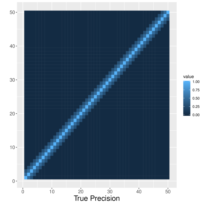
(a) True precision

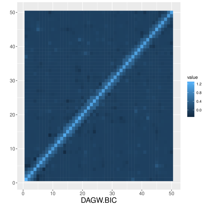
(b) DAGW.BIC

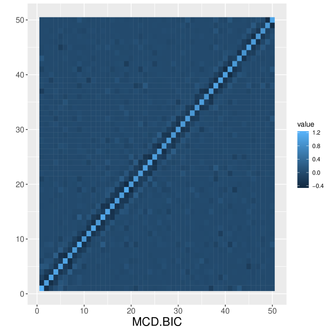
(c) MCD.BIC

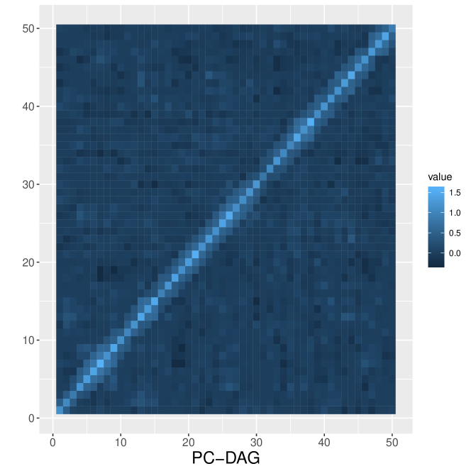
(d) PC-DAG

Figure 2: Heatmap comparison of estimates when $p=50$

References

- Banerjee and Ghosal [2014] S. Banerjee and S. Ghosal. Posterior convergence rates for estimating large precision matrices using graphical models. Electronic Journal of Statistics, 8:2111–2137, 2014.
- Banerjee and Ghosal [2015] S. Banerjee and S. Ghosal. Bayesian structure learning in graphical models. Journal of Multivariate Analysis, 136:147–162, 2015.
- Ben-David et al. [2016] E. Ben-David, T. Li, H. Massam, and B. Rajaratnam. High dimensional bayesian inference for gaussian directed acyclic graph models. Technical Report, http://arxiv.org/abs/1109.4371, 2016.
- Bickel and Levina [2008a] P. J. Bickel and E. Levina. Regularized estimation of large covariance matrices. Ann. Statist., 36:199–227, 2008a.
- Bickel and Levina [2008b] P. J. Bickel and E. Levina. Covariance regularization by thresholding. Ann. Statist., 36(6):2577–2604, 12 2008b. doi: 10.1214/08-AOS600. URL https://doi.org/10.1214/08-AOS600.
- Cao et al. [2019] X. Cao, K. Khare, and M. Ghosh. Posterior graph selection and estimation consistency for high-dimensional bayesian dag models. Ann. Statist., 47(1):319–348, 02 2019.
- Chang and Tsay [2010] Changgee Chang and Ruey S. Tsay. Estimation of covariance matrix via the sparse cholesky factor with lasso. Journal of Statistical Planning and Inference, 140(12):3858 – 3873, 2010.
- El Karoui [2008] N. El Karoui. Spectrum estimation for large dimensional covariance matrices using random matrix theory. Annals of Statistics, 36:2757–2790, 2008.
- Kalisch and Bühlmann [2007] Markus Kalisch and Peter Bühlmann. Estimating high-dimensional directed acyclic graphs with the pc-algorithm. The Journal of Machine Learning Research, 8:613–636, 2007.
- Kang and Deng [2017] X. Kang and X. Deng. An improved modified cholesky decomposition method for inverse covariance matrix estimation. arXiv:1710.05163, 2017.
- Khare et al. [2017] K. Khare, S. Oh, S. Rahman, and B. Rajaratnam. A convex framework for high-dimensional sparse cholesky based covariance estimation in gaussian dag models. Preprint, Department of Statisics, University of Florida, 2017.
- Pourahmadi [2007] M. Pourahmadi. Cholesky decompositions and estimation of a covariance matrix: Orthogonality of variance–correlation parameters. Biometrika, 94:1006–1013, 2007.
- Rütimann and Bühlmann [2009] Philipp Rütimann and Peter Bühlmann. High dimensional sparse covariance estimation via directed acyclic graphs. Electron. J. Statist., 3:1133–1160, 2009.
- Shojaie and Michailidis [2010] A. Shojaie and G. Michailidis. Penalized likelihood methods for estimation of sparse high-dimensional directed acyclic graphs. Biometrika, 97:519–538, 2010.
- van de Geer and Bühlmann [2013] Sara van de Geer and Peter Bühlmann. -penalized maximum likelihood for sparse directed acyclic graphs. Ann. Statist., 41(2):536–567, 04 2013.
- Xiang et al. [2015] R. Xiang, K. Khare, and M. Ghosh. High dimensional posterior convergence rates for decomposable graphical models. Electronic Journal of Statistics, 9:2828–2854, 2015.