Stochastic ejection of nanocontact droplet solitons via drift instability

Abstract

The magnetic droplet soliton is a large amplitude, coherently precessing wave state that exists in ferromagnetic thin films with perpendicular magnetic anisotropy. To effectively sustain a droplet, magnetic damping can be locally compensated in a nanocontact region that imparts spin-transfer torque; this has been successfully deployed in experiment to directly image the droplet and probe its dynamics electrically. However, theory predicts and experiments indicate the existence of a drift instability whereby the droplet is ejected from the spin-transfer-torque-active region and subsequently decays, an effect that may be enhanced or possibly induced by thermal fluctuations. Using soliton perturbation theory and large deviation theory, this work determines the soliton ejection rate and the most likely path an ejected soliton tracks in the presence of thermal fields. These results lead to an effective lower bound on the stability of magnetic droplet solitons in spin-transfer torque nanocontact devices operating at finite temperature and point to ways in which droplets can be made more robust.

I Introduction

The pursuit of fast, scalable nonvolatile storage and new ways to process digital information have motivated much recent study of the formation and control of localized structures in ferromagnetic materials. These structures are supported by an energetic balance among contributions from material anisotropy, exchange energy, dipole or self-induced field energy, and forcing due to external fields, current-induced spin torque, and magnetic damping. Some localized structures, such as skyrmions, are created with a topology that cannot continuously deform to the trivial state, lending promise for additional structural stability in the absence of a driving force. Other structures, such as dissipative solitons, are maintained by a balance between driving and damping terms. In both cases, structures that are stable under deterministic dynamics are generally only quasi-stable under the inevitable influence of thermal fluctuations or other stochastic phenomena.

In this paper, we study the effects of weak thermal fluctuations on the magnetic droplet soliton Kosevich et al. (1990), a large-amplitude, precessing mode that manifests as a balance between nonlinearity due to uniaxial anisotropy and dispersion due to the exchange interaction. Because of the droplet’s precessional dynamics, its practical realization was predicted Hoefer et al. (2010) and then observed both indirectly via the giant magnetoresistance (GMR) effect Mohseni et al. (2013); Macià et al. (2014) and directly with x-ray transmission microscopy Backes et al. (2015); Chung et al. (2018) in a spin-transfer torque driven nanocontact device that imparts a current-induced local torque to compensate uniform magnetic damping. Additional experiments Lendínez et al. (2015); Chung et al. (2016) used the GMR effect to measure the nanocontact device’s frequency characteristics, highlighting a low-frequency signal that was attributed to a drift instability whereby the soliton is expelled from the nanocontact and then decays, after which a new droplet forms under the nanocontact and the process repeats Hoefer et al. (2010). This drift instability presents a significant challenge to the robust control of droplet solitons and the reliable operation of future spintronic devices. Due to growing interest in magnetic droplet solitons, experiments continue in spin torque nanocontacts Xiao et al. (2017); Hang et al. (2018); Chung et al. (2018); Jiang et al. (2018) and in spin Hall driven nanoconstrictions Divinskiy et al. (2017).

The existence and dynamics of droplets in nanocontacts have been successfully described using soliton perturbation theory Bookman and Hoefer (2013, 2015), that yields a system of ordinary differential equations (ODEs) for the droplet’s parameters that we call the modulation equations. The ODEs’ fixed points correspond to sustained droplets, which, for a certain parameter regime, are unstable and manifest an increase in the droplet’s speed, i.e., the drift instability Wills et al. (2016). Their stochastic dynamics under a thermal random field were explored theoretically Wills et al. (2016). The objective of that study was to compute the approximate variance in droplet parameters, including its frequency, linewidth and position relative to the spot of the nanocontact supporting it. The Ornstein-Uhlenbeck process derived from linearizing the stochastic model equations about the dissipative droplet state was shown to provide statistics that agree well with simulations of the nonlinear stochastic model and with micromagnetic simulations performed using open source code MuMax3. That study also contained the description of the aforementioned drift instability occurring at critical bias current.

An equally important figure of merit for magnetic droplets in the presence of a thermal field is the probability (alternatively, the rate) of ejection, where the droplet escapes the attractive potential provided by the finite spatial extent of the nanocontact and then decays due to magnetic damping. In the physically relevant limit of weak thermal effects, exits occur rarely, with a probability or rate determined by large deviation theory. In this limit, the asymptotic scaling of exit probabilities and rates with vanishing noise strength is provided by a rate function related to the exit path or paths that minimize an action functional. This asymptotic scaling provides an order-of-magnitude estimate for the ejection rate, which would otherwise be estimated through sampling using, for example, a software package such as MuMax3 Vansteenkiste et al. (2014). These simulations must resolve dynamics on gyromagnetic time scales of nanoseconds, while our estimates show that exits occur on time scales of micro- to milliseconds, depending on the operating regime. Monte Carlo methods to estimate ejection rates or ejection probabilities over finite times are therefore unreasonably expensive.

In this work, we demonstrate that, even in regimes where the droplet fixed point is nominally stable under deterministic dynamics of the modulation ODEs, the proximity of a saddle point associated with the drift instability provides an important mechanism for droplet ejection. We use a combination of analytical and numerical techniques to compute the action associated with exits through all saddles with a single unstable manifold, including the saddles with nonzero velocity bifurcating through the drift instability Wills et al. (2016) and those associated with zero velocity originating in a saddle-node bifurcation in the precessional frequency Bookman and Hoefer (2013). Our most important physical result is the determination of the mean time it takes for a deterministically stable droplet to be ejected from the nanocontact due to thermal noise. Based on physical parameters from recent experiments Lendínez et al. (2017, 2015), we estimate this time to be approximately 50 nanoseconds or a rate of droplet ejection of 20 MHz, which is within an order of magnitude of low-frequency observations from recent experiments. We estimate that this rate can be manipulated and, importantly, significantly decreased through appropriate choice of operating parameters.

II Model

We study a model for the magnetization ${\bf M}=M_{s}\hat{\bf m}$ of the free layer in a thin magnetic film supported from below by a thin nonmagnetic conducting layer followed by a fixed layer with constant magnetization ${\bf M}_{p}=M_{p}\hat{\bf m}_{p}$, where $M_{s}$ and $M_{p}$ are their respective saturation magnetizations. The fixed layer plays the role of a current polarizer enabling both magnetoresistive detection of the free layer magnetization and switching of the free layer through spin-transfer torque (STT). The current density is approximately restricted in space to a circular disc nanocontact of radius $R_{*}$ placed on top of the free layer. An external field $H_{0}$ is applied perpendicular to the layers in order to provide control over the fixed layer magnetization and to stabilize the droplet.

From the Landau-Lifshitz equations for the free layer normalized magnetization defined on the plane, $\hat{\bf m}({\bf x},t):{\mathbb{R}}^{2}\times{\mathbb{R}}\rightarrow{\mathbb{S}}^{2}$, we have

$$\frac{\partial\hat{\bf m}}{\partial{t}}=-\hat{\bf m}\times{\bf h}_{\mathrm{eff}}-\alpha\hat{\bf m}\times(\hat{\bf m}\times{\bf h}_{\mathrm{eff}})+iH(\rho_{*}-|{\bf x}|)\hat{\bf m}\times(\hat{\bf m}\times\hat{\bf m}_{p})-\hat{\bf m}\times{\bf h},$$ (1)

where $0<\alpha\ll 1$ is the damping parameter, $H(x)$ is the Heaviside function, and $i=I/I_{0}$ is the STT current nondimensionalized by

$$I_{0}=\frac{4\mu_{0}M_{s}(H_{k}-M_{s})e\pi R_{*}^{2}\delta}{\hbar\eta},$$ (2)

with $H_{k}$ the anisotropy field, $\delta$ the free layer thickness, $\eta$ the spin torque efficiency, and $\rho_{*}=R_{*}/L$. In Eqn. 1, time has been nondimensionalized using the precessional time scale $\tau=(|\gamma|\mu_{0}(H_{k}-M_{s}))^{-1}$, where $\gamma$ is the gyromagnetic ratio and $\mu_{0}$ is vacuum permeability. In-plane lengths are normalized by $L=\lambda_{\mathrm{ex}}\sqrt{M_{s}/(H_{k}-M_{s})}$ where $\lambda_{\mathrm{ex}}$ is the exchange length. The respective influences of the external magnetic field $H_{0}=(H_{K}-M_{s})h_{0}$, the exchange field, and perpendicular anisotropy sufficient to exceed the local demagnetizing field contribution ($H_{K}>M_{s}$) are included in

$${\bf h}_{\mathrm{eff}}=h_{0}\hat{\bf z}+\nabla^{2}\hat{\bf m}+m_{z}\hat{\bf z}.$$ (3)

Finally, thermal effects are modeled using the fluctuation-dissipation principle Brown Jr (1963) and are described by the final term in Eqn. 1, which is taken to be space-time white noise with

$${\mathbb{E}}({\bf h}({\bf x},t){\bf h}^{\dagger}({\bf x}^{\prime},t^{\prime}))=\beta^{2}{\bf I}\,\delta({\bf x}-{\bf x}^{\prime})\delta(t-t^{\prime}),$$ (4)

where ${\bf I}$ is the identity matrix, $T$ is temperature, and $\beta^{2}=T/T_{0}$, with

$$T_{0}=\frac{\mu_{0}M_{s}^{2}\lambda_{\mathrm{ex}}^{2}\delta}{2\alpha k_{B}}.$$

It is important to note that the stochastic differential equation (SDE) Eqn. 1 must be interpreted in the sense of Stratonovich to preserve the unit magnitude of $\hat{\bf m}$ ($|\hat{\bf m}({\bf x},t)|=1$ for all ${\bf x}\in{\mathbb{R}}^{2}$, $t\geq 0$).

Following Refs. Bookman and Hoefer (2013), Bookman and Hoefer (2015), and Wills et al. (2016), we express the free-layer magnetization in spherical coordinates such that $\hat{\bf m}=(\sin\Theta\cos\Phi,\sin\Theta\sin\Phi,\cos\Theta)$, with the droplet given approximately by

$$\cos\Theta=\tanh(\rho-1/\omega),$$ (5)

$$\Phi=h_{0}t-\frac{{\bf v}\cdot\hat{\boldsymbol{\rho}}}{\omega^{2}}+\phi,$$ (6)

where $\phi=\omega t+\phi_{0}$ and it is assumed that the precessional frequency $\omega$ above the field-induced frequency $h_{0}$ is small, i.e., $0<\omega<0.25$, and the droplet velocity ${\bf v}$ is small, i.e., $|{\bf v}|\ll\omega$. In this expression, $(\rho,\varphi)$ are polar coordinates centered at the droplet, related to the lab-frame coordinates through ${\bf x}={\boldsymbol{\xi}}+\rho(\cos\varphi,\sin\varphi)$ where ${\boldsymbol{\xi}}_{t}={\bf v}$. Figure 1 illustrates two examples of droplet solitons with the functional form given by (5) and (6). These are described later in the text as centered (left) and non-centered (right) droplet solitons.

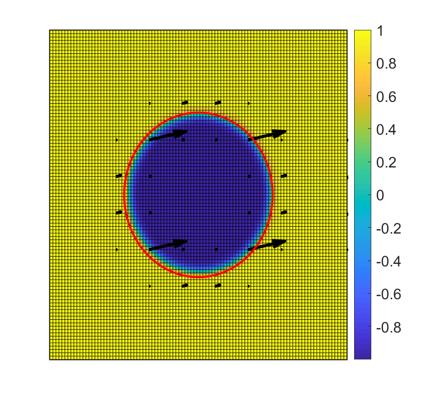
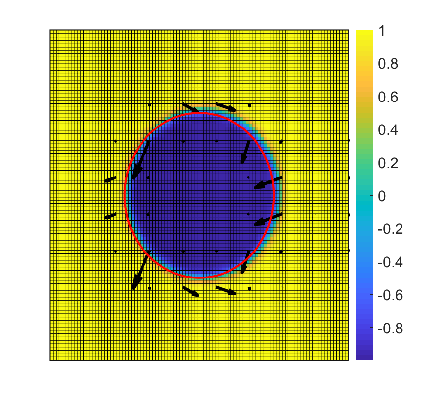
Figure 1: Droplet soliton given by Eqns. 5 and 6. Left image is a centered droplet soliton ($\boldsymbol{\xi}={\bf v}={\bf 0}$), right image is a non-centered droplet soliton ($|\boldsymbol{\xi}|,|{\bf v}|>0$). False color represents out-of-plane component of $\hat{\bf m}$. Arrows represent magnitude and direction of in-plane component of $\hat{\bf m}$, which precesses as time $t$ advances. The red circle is the boundary of the nanocontact.

The droplet is thus characterized by six free parameters: azimuthal phase $\phi_{0}$, position ${\boldsymbol{\xi}}$, precessional frequency $\omega>0$, and velocity ${\bf v}$. It was demonstrated in Ref. Bookman and Hoefer (2015) using soliton perturbation theory in the limit of large nanocontact radius $\rho_{*}\gg 1$, weak damping and STT current $i={\mathcal{O}}(\alpha)\ll 1$, and low temperature $\beta_{0}\ll 1$, that the droplet parameters evolve according to the SDEs

$$d\phi=\omega\,dt+\frac{i}{4\pi}\int_{x\leq\rho_{*}}{\rm sech}\hskip 0.72229pt^{2}(\rho-1/\omega)\,d{\bf x}\,dt+dW_{\phi},$$ (7)

$$d\boldsymbol{\xi}={\bf v}\,dt+\frac{i\omega}{2\pi}\int_{x\leq\rho_{*}}{\rm sech}\hskip 0.72229pt^{2}(\rho-1/\omega)\hat{\boldsymbol{\rho}}\,d{\bf x}\,dt+d{\bf W}_{\xi},$$ (8)

$$d\omega=\alpha\omega^{2}(\omega+h_{0})\,dt-\frac{i\omega^{3}}{4\pi}\int_{x\leq\rho_{*}}{\rm sech}\hskip 0.72229pt^{2}(\rho-1/\omega)\,d{\bf x}\,dt+dW_{\omega},\quad\mbox{and}$$ (9)

$$d{\bf v}=\alpha\omega(\omega+2h_{0}){\bf v}\,dt-\frac{i\omega^{2}}{2\pi}\int_{x\leq\rho_{*}}\left(\frac{3}{2}{\bf v}-\frac{({\bf v}\cdot{\hat{\boldsymbol{\varphi}}})}{\rho\omega}{\hat{\boldsymbol{\varphi}}}\right){\rm sech}\hskip 0.72229pt^{2}(\rho-1/\omega)\,d{\bf x}\,dt+d{\bf W}_{v},$$ (10)

where the process ${\bf W}=(W_{\phi},{\bf W}_{\xi},W_{\omega},{\bf W}_{v})$ satisfies

$${\mathbb{E}}[{\bf W}(t){\bf W}^{\dagger}(t^{\prime})]=\frac{\beta_{0}^{2}}{2\pi}\min(t,t^{\prime})\begin{pmatrix}\begin{matrix}v^{2}/4\omega+\omega/2&{\bf v}^{\dagger}/2\\ {\bf v}/2&\omega{\bf I}_{2\times 2}\end{matrix}&{\bf 0}_{3\times 3}\\ {\bf 0}_{3\times 3}&\begin{matrix}\omega^{5}/2&\omega^{4}{\bf v}^{T}\\ \omega^{4}{\bf v}&{\boldsymbol{\sigma}}_{v}^{2}\end{matrix}\end{pmatrix}$$ (11)

where

$${\bf\sigma}_{v}^{2}=\begin{pmatrix}\omega^{5}+\omega^{3}(9v_{x}^{2}+v_{y}^{2})/4&2\omega^{3}v_{x}v_{y}\\ 2\omega^{3}v_{x}v_{y}&\omega^{5}+\omega^{3}(v_{x}^{2}+9v_{y}^{2})/4\end{pmatrix}.$$ (12)

It should be pointed out that in deriving Eqn. 10 from Eqn. 1 (i.e., from the general modulation equation (4.4) in Ref. Bookman and Hoefer (2015)), the stochastic driving term is not strictly normalizable (i.e., does not have bounded variance) due to the $1/\rho$ contribution in the integrand near $\rho=0$ (the deterministic term does not suffer this difficulty since $1/\rho$ is integrable but not square-integrable). Using the argument that the primary contribution from thermal fluctuations must come from values at the perimeter of the droplet $\rho\approx 1/\omega\gg 1$, however, we disregard the contribution near $\rho=0$ – where the droplet is exponentially close to pointing down – to provide a well-posed diffusion process.

Since no other parameters depend on $\phi$ and since spatial isotropy allows the coordinate frame to be aligned with ${\boldsymbol{\xi}}$ with nothing lost but an irrelevant angle, the full dynamics of Eqns. 7 through 10 are captured by the four-dimensional system

$$d\xi =\left[v_{\parallel}+\frac{i\omega}{\pi}f_{1}(\xi,\omega)\right]\,dt+dW_{\xi},$$ (13)

$$d\omega =\left[\alpha\omega^{2}(\omega+h_{0})-\frac{i\omega^{3}}{2\pi}f_{2}(\xi,\omega)\right]\,dt+dW_{\omega},$$ (14)

$$dv_{\parallel} =\left[\alpha\omega(\omega+2h_{0})-\frac{3i\omega^{2}}{2\pi}f_{2}(\xi,\omega)+\frac{i\omega}{\pi}f_{3}(\xi,\omega)\right]v_{\parallel}\,dt+dW_{\parallel},\quad\mbox{and}$$ (15)

$$dv_{\perp} =\left[\alpha\omega(\omega+2h_{0})-\frac{3i\omega^{2}}{2\pi}f_{2}(\xi,\omega)+\frac{i\omega}{\pi}f_{4}(\xi,\omega)\right]v_{\perp}\,dt+dW_{\perp},$$ (16)

with $v_{\parallel}={\bf v}\cdot{\hat{\boldsymbol{\xi}}}$, $v_{\perp}={\bf v}\cdot{\bf J}{\hat{\boldsymbol{\xi}}}$ where $J=\begin{pmatrix}0&-1\\ 1&0\end{pmatrix}$, and

$${\mathbb{E}}[W(t)W^{T}(t^{\prime})]=\frac{\beta_{0}^{2}}{2\pi}\min(t,t^{\prime})\begin{pmatrix}\omega&0&{\bf 0}^{T}\\ 0&\omega^{5}/2&\omega^{4}{\bf v}^{T}\\ {\bf 0}&\omega^{4}{\bf v}&{\boldsymbol{\sigma}}_{v}^{2}\end{pmatrix}$$ (17)

where

$${\boldsymbol{\sigma}}_{v}^{2}=\begin{pmatrix}\omega^{5}+\omega^{3}(9v_{\parallel}^{2}+v_{\perp}^{2})/4&2\omega^{3}v_{\parallel}v_{\perp}\\ 2\omega^{3}v_{\parallel}v_{\perp}&\omega^{5}+\omega^{3}(v_{\parallel}^{2}+9v_{\perp}^{2})/4\end{pmatrix}$$ (18)

and ${\bf v}=(v_{\parallel},v_{\perp})$.

The nonlocal terms in Eqns. 13 through 16 are given by

$$f_{1}(\xi,\omega)=\frac{1}{2}\int_{x\leq\rho_{*}}\cos\varphi\,{\rm sech}\hskip 0.72229pt^{2}(\rho-1/\omega)\,d{\bf x},$$ (19)

$$f_{2}(\xi,\omega)=\frac{1}{2}\int_{x\leq\rho_{*}}{\rm sech}\hskip 0.72229pt^{2}(\rho-1/\omega)\,d{\bf x},$$ (20)

$$f_{3}(\xi,\omega)=\frac{1}{2}\int_{x\leq\rho_{*}}\frac{\sin^{2}\varphi}{\rho}{\rm sech}\hskip 0.72229pt^{2}(\rho-1/\omega)\,d{\bf x},\quad\mbox{and}$$ (21)

$$f_{4}(\xi,\omega)=\frac{1}{2}\int_{x\leq\rho_{*}}\frac{\cos^{2}\varphi}{\rho}{\rm sech}\hskip 0.72229pt^{2}(\rho-1/\omega)\,d{\bf x}.$$ (22)

The terms in (7) through (10), and consequently (13) through (16), proportional to $\alpha$ or $i$ correspond to contributions from magnetic damping or STT, respectively.

We study the above model using the parameters contained in Refs. Lendínez et al. (2015) and Lendínez et al. (2017), where $R_{*}=75$ nm, $\mu_{0}M_{s}=0.95$ T, $\mu_{0}H_{k}=1.2$ T, $\lambda_{ex}=5.3$ nm, $\mu_{0}H_{0}\in(0.2,1.4)$ T, $\delta=5$ nm, $\eta=0.26$, $\tau=0.13$ ns, $\alpha=0.03$, and $T=314$ K. These parameters produce dimensionless parameters equal to $h_{0}\in(0.8,5.6)$, $\rho_{*}=7.3$, and $\beta^{2}=2.6\times 10^{-3}$.

III Large deviation theory

Stochastic dynamical systems in the form of the Ito diffusion

$$d{\bf u}={\bf f}({\bf u})\,dt+\epsilon\beta({\bf u})\,d{\bf W}$$ (23)

have long been the subject of study in physical systems where rare events are important phenomena to understand. It is now well understood Freidlin and Wentzell (2012) that, in the limit as $\epsilon\rightarrow 0$, the probability of paths connecting any two states ${\bf u}_{1}$ and ${\bf u}_{2}$ approaches zero with a scaling that is exponential in $\epsilon^{2}$. The rate of this asymptotic decay is dictated by minimizers of the Wentzell-Freidlin action functional,

$$S_{T}[{\bf u}(t)]=\int_{0}^{T}\frac{1}{2}\left(\dot{\bf u}-{\bf f}({\bf u})\right)^{T}(\beta\left({\bf u})\beta({\bf u})^{T}\right)^{-1}\left(\dot{\bf u}-{\bf f}({\bf u})\right)\,dt$$ (24)

where the admissible set includes all absolutely continuous paths ${\bf u}(t)$ connecting ${\bf u}_{1}$ and ${\bf u}_{2}$.

In the case of an exit from the basin of attraction of a deterministically stable fixed point, the time $T$ over which the exit occurs clearly plays an important role in determining the probability of exit. If $\Omega$ is the basin of attraction of a fixed point ${\bf u}_{0}$, then

$$\lim_{\epsilon\rightarrow 0}\epsilon^{2}\log{\mathbb{P}}({\bf u}(T)\in\Omega)=-\min_{{\bf u}(T)\in\Omega\cup\partial\Omega}S_{T}[{\bf u}(t)],$$

$$\lim_{\epsilon\rightarrow 0}\epsilon^{2}\log{\mathbb{P}}(t_{E}\leq T)=-\min_{{\bf u}(s)\notin\Omega,\,s\leq T}S_{T}[{\bf u}(t)],$$

where $t_{E}=\min(t:{\bf u}(t)\notin\Omega)$ is defined as the first time of exit and $\partial\Omega$ is the boundary of $\Omega$.

Over arbitrary long time scales, exits occur with probability one. The question is therefore not whether an exit will occur, but rather how long one should expect to wait before it does. The mean time to exit (MTE) can be shown to increase exponentially as $\epsilon$ decreases, with a rate dictated by the action $S_{T}$ minimized over all possible transit times. With the action left only as a function of state space, one can define a “quasi-potential” function that quantifies the MTE from ${\bf u}_{0}$ to any other state ${\bf u}$, i.e. $Q({\bf u})=\inf_{T}S_{T}$, where $S_{T}$ is the minimizer of $S_{T}[{\bf u}(t)]$ over continuous paths ${\bf u}(t)$ satisfying ${\bf u}(0)={\bf u}_{0}$ and ${\bf u}(T)={\bf u}$. In particular,

$$\lim_{\epsilon\rightarrow 0}\epsilon^{2}\log\mathbb{E}[t_{E}]=\inf_{{\bf u}\in\partial\Omega}Q({\bf u}).$$ (25)

Under broad conditions, minima of the quasi-potential occur at 1-saddles, which represent the most likely points of exit from the basin of attraction of the stable fixed point.

Gradient flows (23) where ${\bf f}({\bf u})=-\nabla V({\bf u})$ for some potential function $V({\bf u})$ represent a special case in the theory of large deviations. In this case, it can be shown Freidlin and Wentzell (2012) that the quasi-potential between a minimum of $V$ and the nearest saddle point is simply given by twice the difference in potential between the two points. One-dimensional SDEs are automatically gradient flows since one can simply define

$$V(u)=-\int_{u_{0}}^{u}f(y)\,dy.$$ (26)

While the above consideration provides the exponential scaling law for transition probabilities and mean times to exit, a more detailed analysis is required Gardiner ; Forgoston and Moore (2018); Matkowsky and Schuss (1977) to improve on this estimate by providing the prefactor of the exponential, for example. In this work we discuss only the rate function, leaving a more accurate approximation for further study.

IV Deterministic dynamics

In the four-dimensional system described by Eqns. 13 through 16, the first three parameters only depend on $v_{\perp}$ through the diffusion tensor. A complete description of the deterministic dynamics is therefore afforded by the reduced system

$$\dot{\xi} =v_{\parallel}+{i\omega}{\pi}f_{1},$$ (27)

$$\dot{\omega} =\alpha\omega^{2}(\omega+h_{0})-\frac{i\omega^{3}}{2\pi}f_{2},$$ (28)

$$\dot{v}_{\parallel} =\left[\alpha\omega(\omega+2h_{0})-\frac{3i\omega^{2}}{2\pi}f_{2}+\frac{i\omega}{\pi}f_{3}\right]v_{\parallel}.$$ (29)

The case $v_{\parallel}=0$ has been thoroughly studied in Ref. Bookman and Hoefer (2013), where it was shown that multiple fixed points are possible with $\xi=v_{\parallel}=0$ depending on the number of roots of

$$\Gamma(\omega):=\alpha(\omega+h_{0})-\frac{1}{2}i\omega\left[\rho_{*}\tanh\left(\rho_{*}-\frac{1}{\omega}\right)-\ln\cosh\left(\rho_{*}-\frac{1}{\omega}\right)+\ln\cosh\frac{1}{\omega}\right],$$ (30)

where we note that $\Gamma(0^{+})=\alpha h_{0}>0$. Figure 2 illustrates the zero-level surface of $\Gamma(\omega)$ for different values of the applied field $h_{0}$ and scaled STT current $i/\alpha$ for $\rho_{*}=7.3$. Considering for a moment the 2d system where we restrict $v_{\parallel}=0$ and fix a small applied field $h_{0}$, a saddle-node bifurcation occurs for $i/\alpha\approx h_{0}$ and the saddle approaches infinity as $i/\alpha$ approaches $2/\ln 2$. For larger values of applied field, another stable fixed point bifurcates from infinity either before or after the original saddle-node bifurcation to collide with and annihilate the saddle as $i/\alpha$ is increased.

Figure 2: Zero-level surface of $\Gamma(\omega;i/\alpha,h_{0})$ for $\rho_{*}=7.3$.

Since $\mathrm{sgn}\,(f_{1})=-\mathrm{sgn}\,(\xi)$ (see Appendix), fixed points satisfy $v_{\parallel}=0$ if and only if $\xi=0$. Centered droplet solitons, depicted in the left image of Fig. 1, satisfy $\xi=v_{\parallel}=0$ while non-centered droplet solitons, depicted in the right image, satisfy $\xi\neq 0$ and $v_{\parallel}\neq 0$.

The full stability of the centered fixed points is dictated by the Jacobian evaluated at $(0,\omega_{*},0)$,

$$J=\begin{pmatrix}\lambda_{1}&0&1\\ 0&\lambda_{2}&0\\ 0&0&\lambda_{3}\end{pmatrix},$$ (31)

where

$$\lambda_{1}=-\frac{1}{2}\rho_{*}i\omega\,{\rm sech}\hskip 0.72229pt^{2}(\rho_{*}-1/\omega),$$ (32)

$$\lambda_{2}=\lambda_{1}-\alpha h_{0}\omega+\frac{1}{2}i\omega\left(\tanh(\rho_{*}-1/\omega)+\tanh(1/\omega)\right),$$ (33)

$$\lambda_{3}=\lambda_{2}-\lambda_{1}-2\alpha\omega^{2}.$$ (34)

Bifurcation to the drift instability described in Ref. Wills et al. (2016) occurs when $i/\alpha$ is sufficiently large to force $\lambda_{3}>0$, which occurs when

$$\frac{i}{\alpha}=\frac{2(2\omega_{*}+h_{0})}{\tanh(\rho_{*}-1/\omega_{*})+\tanh(1/\omega_{*})}.$$ (35)

The tangent direction of this unstable manifold is

$$\psi_{3}=\begin{pmatrix}1&0&\frac{1}{2}\rho_{*}i\omega_{*}{\rm sech}\hskip 0.72229pt^{2}(\rho_{*}-1/\omega_{*})\end{pmatrix},$$ (36)

providing an indication of the ejection mechanism associated with the drift instability.

Analysis of non-centered fixed points with $v_{\parallel}\neq 0$ ($\xi\neq 0$) is greatly simplified by the fact that they satisfy a two-dimensional algebraic system

$$\frac{\alpha}{i}(\omega+h_{0})-\frac{\omega}{2\pi}f_{2}(\xi,\omega)=0,$$ (37)

$$\frac{\alpha}{i}(2\omega+h_{0})-\frac{1}{\pi}f_{3}(\xi,\omega)=0$$ (38)

with the velocity then provided by

$$v_{\parallel}=-\frac{i\omega}{\pi}f_{1}(\xi,\omega).$$ (39)

Rather than computing fixed points $(\xi,\omega,v_{\parallel})$ associated with relevant parameter combinations $(\alpha,i,h_{0})$, it is convenient to compute the unique parameter sets $(i/\alpha,h_{0})$ associated with each potential fixed point in the $(\xi,\omega)$ plane and verify that the parameters are within the appropriate asymptotic regime for perturbation theory to be applicable. Thus, the subset of non-centered fixed points plotted in Fig. 3 versus $\xi$ and $\omega$ that correspond to physically relevant values of $i/\alpha$ and $h_{0}$ result in Figs. 4, 5, and 6.

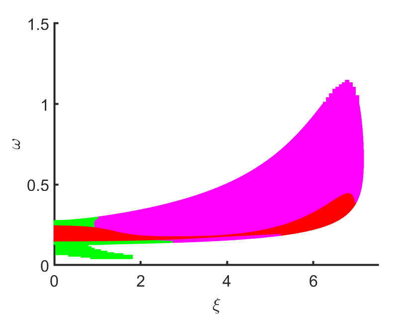
Figure 3: Phase diagram of non-centered fixed points plotted vs. $\xi$ and $\omega$ and color-coded by stability (green is stable; red and magenta correspond to one- and two-dimensional unstable manifolds, respectively). Whitespace region corresponds to unphysical (i.e., negative) values of $i/\alpha$ or $h_{0}$. Slight pixelation for small and large values of $\omega$ reflect lower resolution of computational grid in those regions.

Each of these images is in fact a surface resolved through a set of points using the method described above, where the uniform grid defined in the $(\xi,\omega)$ plane is plainly visible. The color-coded points indicate stability, with green denoting stable fixed points, red denoting fixed points with a one-dimensional unstable manifold (referred to here as 1-saddles), and magenta denoting fixed points with a two-dimensional unstable manifold. The $(i/\alpha,h_{0})$-plane at the base of each graph illustrates the dashed lines $i=\alpha h_{0}$, which provides an approximate lower bound for existence of the centered equilibrium, and the value $i=2\alpha h_{0}$. The solid line is the drift bifurcation curve, computable using Eqn. 35, from which it can be seen that all non-centered fixed points emerge. At small values of $h_{0}$, the bifurcation is supercritical in $i/\alpha$ such that the centered equilibrium immediately transfers its stability to the new non-centered equilibrium. For larger values of $h_{0}$, however, the bifurcation is subcritical in $i/\alpha$, with a sheet of saddles having only one unstable direction in close proximity to the stable centered equilibria. These present the primary ejection mechanism when thermal effects are included, and will be discussed in the next section.

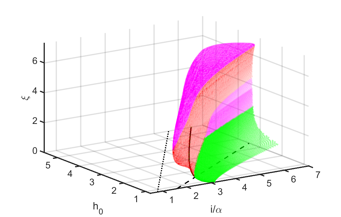
Figure 4: Families of non-centered fixed points color-coded by stability (green is stable; red and magenta correspond to one- and two-dimensional unstable manifolds, respectively) for $\rho_{*}=7.3$. Each bifurcates from the drift instability identified in Wills et al. (2016) (solid black) at $\xi=0$ and moves with increasing position $\xi$ to accumulate in the region (demarcated by dotted and dashed black lines) identified asymptotically in Eqn. (47). Multiple fixed points can exist for each parameter pair $(i/\alpha,h_{0})$, including in the region where $(0,\omega_{*},0)$ is stable.

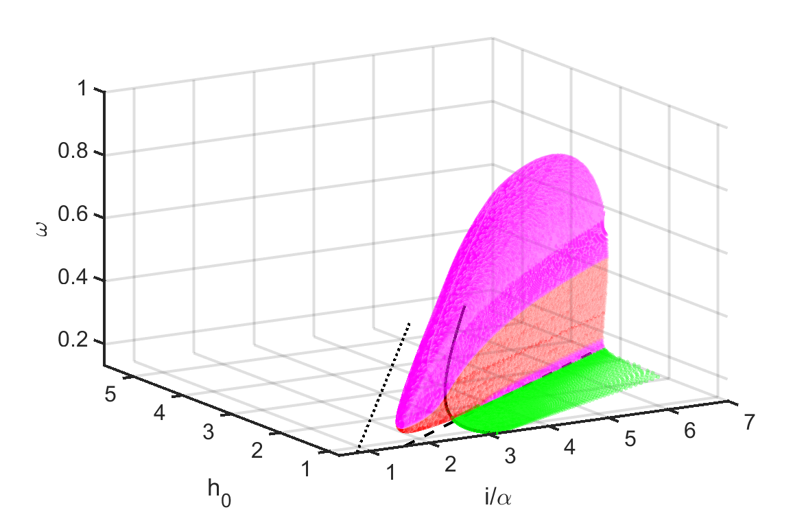
Figure 5: Graph of $\omega$-values associated with the fixed points depicted in Fig. 4, emerging from $\omega=\omega_{*}$ at the drift bifurcation curve and accumulating in the region identified in Eqn. 47. Color coding is the same as in Figs. 3 and 4.

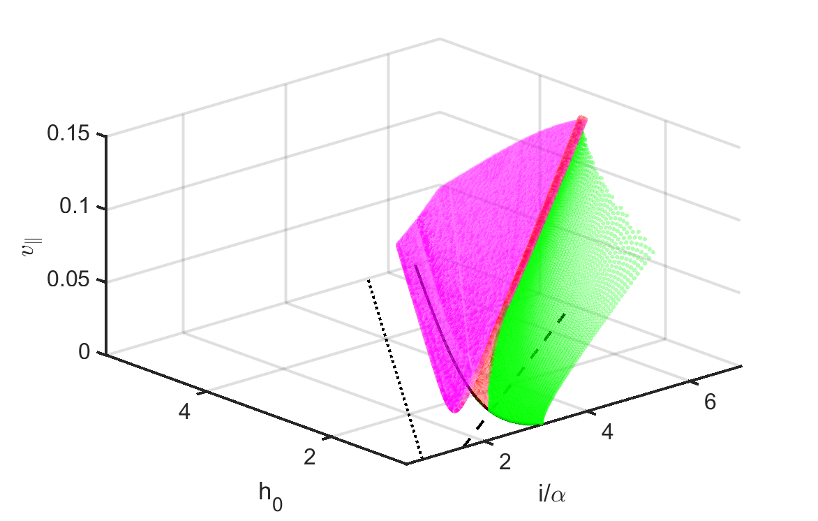
Figure 6: Graph of $v_{\parallel}$-values associated with the fixed points depicted in Fig. 4, emerging from $v_{\parallel}=0$ at the drift bifurcation curve and accumulating in the region identified in Eqn. 47. Color coding is the same as in Figs. 3 and 4.

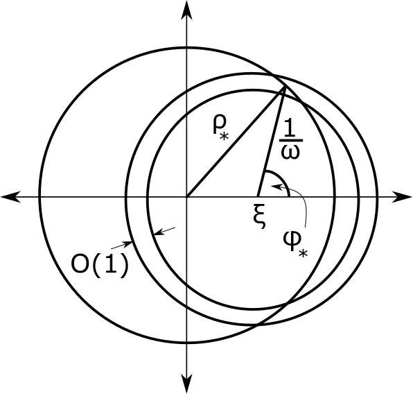
Figure 7: Illustration of geometry used in asymptotic approximation of non-centered fixed point. Soliton-nanocontact interaction only occurs in the portion of the annular region (droplet soliton) that lies inside the zero-centered circle (nanocontact).

An alternative to the strategy above for solving Eqns. 37 and 38 that provides additional insight is to consider them asymptotically for large $\rho_{*}$ and small $\omega$ (i.e., the regime of validity for Eqns. (27) through (29)). We observe in that case that the support of each integral lies in the intersection between the circular disk of radius $\rho_{*}$ and a “washer” with ${\mathcal{O}}(1)$ width and central radius $1/\omega$, with the disk and washer centers separated by $\xi$, as depicted in Fig. 7. The two points of intersection lie at angles $\pm\varphi_{*}$ satisfying

$$\cos(\varphi_{*})=\frac{\omega}{2\xi}\left(\rho_{*}^{2}-\frac{1}{\omega^{2}}-\xi^{2}\right),$$

so that by moving into droplet-centered coordinates, we have

$$\int_{x\leq\rho_{*}}{\rm sech}\hskip 0.72229pt^{2}(\rho-1/\omega)\,d{\bf u} \approx\int_{\varphi_{*}}^{2\pi-\varphi_{*}}\int_{-\infty}^{\infty}{\rm sech}\hskip 0.72229pt^{2}(\rho-1/\omega)\rho\,d\rho\,d\varphi$$ (40)

$$\approx\frac{4}{\omega}(\pi-\varphi_{*}),$$ (41)

where $0\leq\varphi_{*}<\pi$ by construction. The implicit assumption in this construction is that the disk and annulus have nontrivial intersection, which approximately equates to the condition

$$|\xi-\rho_{*}|<1/\omega<\xi+\rho_{*}.$$ (42)

Treating the remaining integrals similarly, we have that

$$\pi\frac{\alpha}{i}(\omega+h_{0})\approx\pi-\varphi_{*},$$ (43)

$$\pi\frac{\alpha}{i}(2\omega+h_{0})\approx\pi-\varphi_{*}+\frac{1}{2}\sin 2\varphi_{*}.$$ (44)

Equating expressions for $\omega$ thus gives

$$\sin 2\varphi_{*}=2(\pi-\varphi_{*}-\pi\alpha h_{0}/i).$$ (45)

From Eqn. 43, we require that $\pi-\varphi_{*}>\pi\alpha h_{0}/i$, so that

$$0\leq\varphi_{*}\leq\pi/2,$$ (46)

which confines the droplet center to within the nanocontact (see Fig. 7). Thus

$$\alpha h_{0}<i<2\alpha h_{0}$$ (47)

for existence of this fixed point. Figures 4 through 6 clearly demonstrate that the surface of fixed points emerging from the drift bifurcation accumulates within this region. Moreover, it is only within this region that the drift bifurcation is subcritical, such that the region where a stable fixed point coexists with a saddle point associated with the drift mode is the intersection of (47) and the half-plane bounded by (35).

The unique solution for $\varphi_{*}$ produces non-centered fixed points with approximate values

$$\omega_{v}\approx\frac{i}{\alpha}\left(1-\frac{\varphi_{*}}{\pi}\right)-h_{0}\quad\mbox{and}$$ (48)

$$\xi_{v}\approx\sqrt{\rho_{*}^{2}-\frac{\sin^{2}\varphi_{*}}{\omega_{v}^{2}}}-\frac{\cos\varphi_{*}}{\omega_{v}}.$$ (49)

Both of these quantities are positive. The associated parallel velocity is provided by

$$v_{v}\approx\frac{2i}{\pi}\sin\varphi_{*},$$ (50)

which is well-approximated near the critical line $i=\alpha h_{0}$ by

$$v_{v}\approx i\left(\frac{i}{\alpha h_{0}}-1\right).$$ (51)

The perpendicular velocity $v_{\perp}$ associated with non-centered fixed points is $v_{\perp}=0$. Hence, for each $(\omega_{v},\xi_{v},v_{v})$ fixed point, there is a corresponding collection of fixed points for the original six-dimensional dynamical system (7-10) with droplet positions ${\boldsymbol{\xi}}$ on the circle $|{\boldsymbol{\xi}}|=\xi_{v}$. Having identified all centered and non-centered fixed points, we now turn to the calculation of the action of paths connecting them.

V Action and optimal paths

In the limit of vanishing noise strength, exits from the basin of attraction of a stable fixed point collapse at an exponentially growing probability onto paths that lead to the nearest 1-saddle, where proximity is defined using a metric weighted by the diffusion tensor. In the four-dimensional system given by Eqns. 13 through 16, there are two candidates for the saddle that represent the most likely exit point, either a decay mode or a drift mode. We study these in turn to identify their associated limiting exit rates.

The first saddle is that identified at $\xi=v=0$ for values of $i/\alpha$ that lie between the saddle-node bifurcation occurring at approximately $i/\alpha=h_{0}$ and the value of $i/\alpha$ where the saddle either runs off to infinity (for small values of $h_{0}$) or is destroyed in a saddle-node bifurcation with another stable fixed point (for sufficiently large values of $h_{0}$). Labelling the centered stable fixed point by $(0,\omega_{*},0)$ and the saddle by $(0,\omega_{s},0)$, we postulate based on the form of the action (24) and numerical results that optimal paths connecting these two fixed points with optimal action $S$ satisfy $\xi=|{\bf v}|=0$. Dependence of the diffusion tensor on the state variables precludes a definite statement that this is true, but we have observed it in all cases we have computed. Since this exit mechanism occurs strictly via changes in $\omega$, thereby mimicking the impact of damping on solitons Bookman and Hoefer (2013), we refer to it as a decay mode of exit.

If we assume this to be true, the action collapses to

$$S=\int_{-\infty}^{\infty}L\,dt\qquad\mbox{with}\qquad L=\frac{2\pi}{\omega^{5}}[\dot{\omega}-\omega^{2}\Gamma(\omega)]^{2}.$$ (52)

where, by construction, $\Gamma(\omega)\leq 0$ if $\omega_{*}\leq\omega\leq\omega_{s}$ and equality holds only at the endpoints. As explained on p. 26, one-dimensional flows are trivially gradient flows and it is immediate that optimal paths satisfy

$$\dot{\omega}=-\omega^{2}\Gamma(\omega),$$ (53)

which integrates to give the Wentzell-Freidlin action

$$S=Q(\omega_{s})-Q(\omega_{*})$$ (54)

where $Q$ is the quasi-potential defined by

$$Q(\omega) =-8\pi\int\frac{\Gamma(\omega)}{\omega^{3}}\,d\omega$$

$$=4\pi\left(\frac{h_{0}\alpha-i}{\omega^{2}}+\frac{2\alpha}{\omega}+\rho_{*}i\ln\frac{\cosh(\rho_{*}-1/\omega)}{\cosh\rho_{*}}+\frac{\rho_{*}i}{\omega}\right.$$

$$\left.-\frac{i}{2}\left[\mathrm{Li}\,_{2}(-e^{-2(\rho_{*}-1/\omega)})+\mathrm{Li}\,_{2}(-e^{-2/\omega})-\mathrm{Li}\,_{2}(-e^{-2\rho_{*}})+\frac{\pi^{2}}{12}\right]\right)$$ (55)

with $\mathrm{Li}\,_{2}(z)$ the dilogarithm function defined by

$$\mathrm{Li}\,_{2}(z)=-\int_{0}^{z}\ln(1-t)\frac{dt}{t}.$$ (56)

The quasi-potential (55) has been defined such that $\lim_{\omega\rightarrow\infty}Q(\omega)=0$. As explained earlier, depending on the parameters $h_{0}$ and $i/\alpha$, the saddle point $(0,\omega_{s},0)$ may not exist. In these cases, we identify an exit via the decay mode with $\omega\rightarrow\infty$, such that the associated Wentzell-Freidlin action simplifies to $S=-Q(\omega_{*})$. As illustrated in Fig. 8, expression (55) for the quasipotential $Q$ blows up as $\omega\rightarrow 0$. This is expected since the noise strength goes to zero as $\omega\rightarrow 0$.

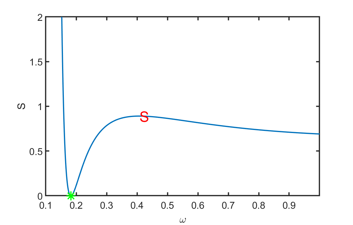
Figure 8: Quasipotential given in Eqn. 55 for $\rho_{*}=7.3$, $i/\alpha=6$, $h_{0}=5.6$. Green star and red “S” denote stable fixed point and saddle, respectively. $Q$ blows up as $\omega\rightarrow 0^{+}$.

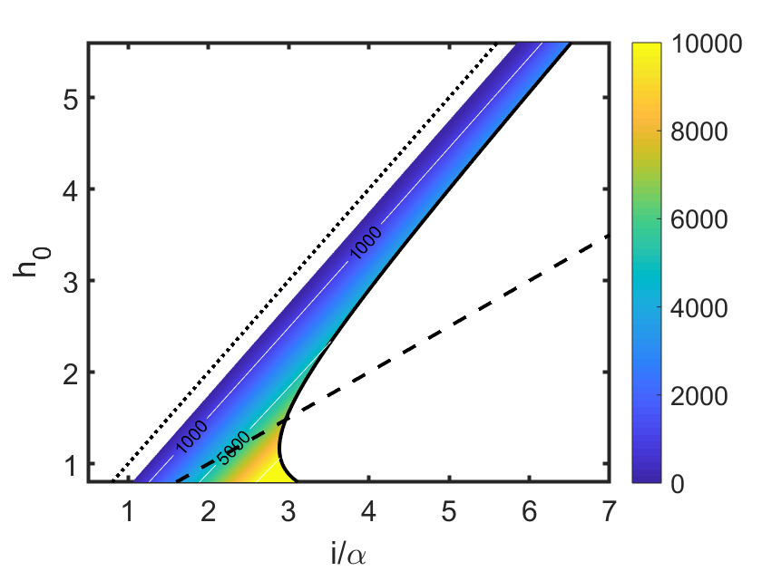
Figure 9: Log of MTE (in dimensionless time units) corresponding to annihilation of the droplet soliton via noise-induced damping. Except for parameters close to the dotted line approximating the existence boundary for the stable centered fixed point, the MTE from this damping mechanism is effectively infinite.

Figure 9 depicts the Wentzell-Freidlin action (54) for different relative STT currents $i/\alpha$ and different applied magnetic fields $h_{0}$. Moving from the dotted line, which provides a lower bound on values of $i/\alpha$ for which the centered droplet exists, toward the solid line, at which the centered droplet loses stability via the drift bifurcation, the MTE is observed to increase very quickly, becoming effectively infinite for parameters not within a very small margin of the dotted line.

Computing the minimum action between the stable fixed point and the saddle with nonzero velocity requires, in principle, consideration of the four-dimensional system given by Eqns. 13 through 16 due to the dependence of the diffusion tensor given by Eqn. 17 on $v_{\perp}$. The contribution from nonzero $v_{\perp}$ is expected to be negligible because $v_{\perp}=0$ at all fixed points, however. For simplicity, we therefore restrict our computations to the minimizers of the action restricted to three-dimensional dynamics, giving

$$S=\int_{-\infty}^{\infty}\frac{1}{2}\left(\dot{\bf u}-{\bf f}({\bf u})\right)^{T}(\beta\left({\bf u})\beta({\bf u})^{T}\right)^{-1}\left(\dot{\bf u}-{\bf f}({\bf u})\right)\,dt$$ (57)

where ${\bf u}=(\xi,\omega,v_{\parallel})$,

$${\bf f}=\begin{pmatrix}v_{\parallel}+\frac{i\omega}{\pi}f_{1}(\xi,\omega)\\ \alpha\omega^{2}(\omega+h_{0})-\frac{i\omega^{3}}{2\pi}f_{2}(\xi,\omega)\\ \left[\alpha\omega(\omega+2h_{0})-\frac{3i\omega^{2}}{2\pi}f_{2}(\xi,\omega)+\frac{i\omega}{\pi}f_{3}(\xi,\omega)\right]v_{\parallel}\end{pmatrix}.$$ (58)

The diffusion tensor appearing in Eqn. 57 is

$$\beta\beta^{T}=\frac{1}{2\pi}\begin{pmatrix}\omega&0&0\\ 0&\omega^{5}/2&\omega^{4}v_{\parallel}\\ 0&\omega^{4}v_{\parallel}&\omega^{5}+\frac{9}{4}\omega^{3}v_{\parallel}^{2}\end{pmatrix}.$$ (59)

The drift ${\bf f}({\bf u})$ is not, in general, either gradient or trivially non-gradient and the action must therefore be computed numerically. The left image in Fig. 10 depicts the approximate MTE obtained by using (25) with the action computed using the generalized minimum action method (or GMAM, see Ref. Heymann and Vanden-Eijnden (2008) for details) at parameter values where the base stationary state is stable and coexists with the saddle corresponding to the drift mode. As explained on p. 47 and observed in Figs. 4 through 6, for a given nanocontact radius $\rho_{*}$, this is approximately the set of current values $h_{0}<i/\alpha<2h_{0}$.

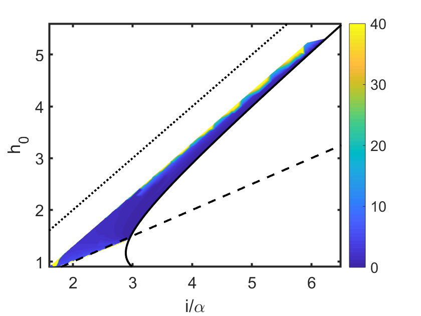
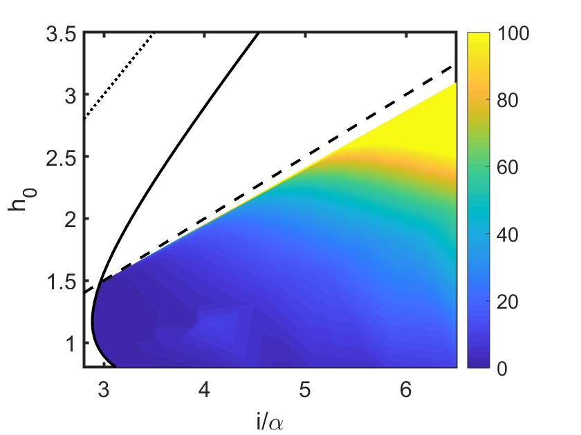
Figure 10: Log of MTE (in dimensionless time units) corresponding to annihilation of the droplet soliton via the drift instability. Left: MTE from stable centered fixed points through non-centered saddle points. Note that the simultaneous existence (i.e., for the same values of $i/\alpha$ and $h_{0}$) of these two fixed points dictates the parameters for which this calculation is relevant (see Fig. 4). Right: MTE from stable non-centered fixed points through centered saddle points. This calculation is relevant for a different region of parameter space. Note that the exit times associated with this droplet annihilation mechanism are much lower than the exit times shown in Fig. 9, and these events are therefore much more likely to be observed on any finite time scale.

The right image in Fig. 10 is the approximate MTE associated with leaving the basin of attraction of stable non-centered fixed points through the now-unstable centered fixed point.

In the parameter regime operable in Fig. 9 and the left image of Fig. 10, the droplet soliton is potentially destroyed via two candidate noise-related mechanisms. The first is the drift mechanism described above, where the position and precessional frequency are driven by noise to the point where the droplet loses stability to a transient traveling droplet which is then ejected from the nanocontact. The MTE associated with this mechanism is plotted on the left in Fig. 10. The second is the decay mode described earlier, whereby an improbable accumulation of fluctuations that drive its precessional frequency sufficiently high as to fall into a regime where damping is no longer counterbalanced by the current passing through the nanocontact. The stochastic dynamics of this mechanism has an associated MTE depicted in Fig. 9. It is clear from this comparison that the action associated with the drift mode is substantially smaller for all parameters investigated here, indicating that this is by far the most dominant mechanism for exit of a centered droplet soliton over the range of values of magnetic field $h_{0}$ and rescaled current $i/\alpha$ for which the original fixed point is stable and the saddle associated with the drift mode exists and has a one-dimensional unstable manifold. As discussed earlier, this is true for a subset of rescaled current values satisfying $i/\alpha<2h_{0}$. For large current but small external field $h_{0}$, where the non-centered fixed points are stable, it appears that the only exit mechanism for those non-centered droplets is through the centered saddle point with a MTE somewhat higher than the exit times associated with annihilation of centered droplets; see Fig. 10, right for the MTE associated with this ejection mechanism.

VI Conclusions

Perturbation theory for a droplet soliton that experiences uniform magnetic damping, local spin transfer torque via a nanocontact, a vertical applied field, and thermal fluctuations, results in a six-dimensional system of stochastic ordinary differential equations. In this paper, we have reduced this system to an equivalent—in the deterministic case—or approximately equivalent—in the stochastic case—three-dimensional system that is amenable to detailed analysis. We completely determined the nature of the fixed points for this dynamical system. One family of fixed points, called nanocontact-centered, exist and are deterministically stable in a restricted regime of current and applied field. These fixed points represent dissipative droplet solitons centered within the nanocontact and precessing at a fixed frequency. In addition to previously studied nanocontact-centered fixed points, we also identify a new class of non-centered fixed points. These latter fixed points correspond to droplet solitons whose centers are displaced relative to the center of the nanocontact, with the resulting force balanced by an anisotropy in the soliton’s in-plane magnetization. These non-centered fixed points are stable in an appropriate parameter regime, but we have not found any parameters at which the centered and non-centered droplet solitons are simultaneously stable. By combining our fixed point analysis with large deviation theory, we identify the mostly likely path through phase space along which a droplet subject to weak thermal noise is expected to decay. A direct computation of the Wentzell-Freidlin action shows that the most likely decay process for stochastically perturbed, centered droplet fixed points is to drift out of the nanocontact. The computed action also provides an estimate for the rate of droplet expulsion from the nanocontact, which sets an effective lower bound for droplet stability in these devices at finite temperature. Based on the parameter values in Refs. Lendínez et al. (2017) and Lendínez et al. (2015), with a time scale $\tau=0.13$ ns, the left image of Fig. 10 yields an estimated droplet ejection rate of $1/(\tau e^{6})\approx 19~{}\mathrm{MHz}$ at room temperature. This rate is an order of magnitude lower than the low-frequency observations in experiments that have been in the 100-500 MHz range. It is important to note that estimates obtained by computing just the Wentzell-Freidlin action (24) provide the scaling law of the MTE in the limit of small noise strength but neglect prefactors that can be large.

References

- Kosevich et al. (1990) A. M. Kosevich, B. A. Ivanov, and A. S. Kovalev, Phys. Rep. 194, 117 (1990).
- Hoefer et al. (2010) M. A. Hoefer, T. J. Silva, and M. W. Keller, Physical Review B 82 (2010), 10.1103/PhysRevB.82.054432.
- Mohseni et al. (2013) S. M. Mohseni, S. R. Sani, J. Persson, T. N. A. Nguyen, S. Chung, Y. Pogoryelov, P. K. Muduli, E. Iacocca, A. Eklund, R. K. Dumas, S. Bonetti, A. Deac, M. A. Hoefer, and J. Akerman, Science 339, 1295 (2013).
- Macià et al. (2014) F. Macià, D. Backes, and A. D. Kent, Nature Nanotechnology 9, 992 (2014).
- Backes et al. (2015) D. Backes, F. Macià, S. Bonetti, R. Kukreja, H. Ohldag, and A. Kent, Physical Review Letters 115 (2015), 10.1103/PhysRevLett.115.127205.
- Chung et al. (2018) S. Chung, Q. T. Le, M. Ahlberg, A. A. Awad, M. Weigand, I. Bykova, R. Khymyn, M. Dvornik, H. Mazraati, A. Houshang, S. Jiang, T. N. A. Nguyen, E. Goering, G. Schütz, J. Gräfe, and J. Åkerman, Phys. Rev. Lett. 120, 217204 (2018).
- Lendínez et al. (2015) S. Lendínez, N. Statuto, D. Backes, A. D. Kent, and F. Macià, Physical Review B 92 (2015), 10.1103/PhysRevB.92.174426.
- Chung et al. (2016) S. Chung, A. Eklund, E. Iacocca, S. M. Mohseni, S. R. Sani, L. Bookman, M. A. Hoefer, R. K. Dumas, and J. Åkerman, Nat. Commun. 7, 11209 (2016).
- Xiao et al. (2017) D. Xiao, V. Tiberkevich, Y. H. Liu, Y. W. Liu, S. M. Mohseni, S. Chung, M. Ahlberg, A. N. Slavin, J. Åkerman, and Y. Zhou, Phys. Rev. B 95, 024106 (2017).
- Hang et al. (2018) J. Hang, C. Hahn, N. Statuto, F. Macià, and A. D. Kent, Scientific Reports 8 (2018), 10.1038/s41598-018-25134-z.
- Jiang et al. (2018) S. Jiang, S. Chung, Q. T. Le, H. Mazraati, A. Houshang, and J. Åkerman, Physical Review Applied 10, 054014 (2018).
- Divinskiy et al. (2017) B. Divinskiy, S. Urazhdin, V. E. Demidov, A. Kozhanov, A. P. Nosov, A. B. Rinkevich, and S. O. Demokritov, Phys. Rev. B 96, 224419 (2017).
- Bookman and Hoefer (2013) L. D. Bookman and M. A. Hoefer, Physical Review B 88 (2013), 10.1103/PhysRevB.88.184401.
- Bookman and Hoefer (2015) L. D. Bookman and M. A. Hoefer, Proceedings of the Royal Society A: Mathematical, Physical and Engineering Science 471, 20150042 (2015).
- Wills et al. (2016) P. Wills, E. Iacocca, and M. A. Hoefer, Physical Review B 93 (2016), 10.1103/PhysRevB.93.144408.
- Vansteenkiste et al. (2014) A. Vansteenkiste, J. Leliaert, M. Dvornik, M. Helsen, F. Garcia-Sanchez, and B. Van Waeyenberge, AIP Advances 4, 107133 (2014).
- Lendínez et al. (2017) S. Lendínez, J. Hang, S. Vélez, J. M. Hernández, D. Backes, A. D. Kent, and F. Macià, Physical Review Applied 7 (2017), 10.1103/PhysRevApplied.7.054027.
- Brown Jr (1963) W. F. Brown Jr, Physical Review 130, 1677 (1963).
- Freidlin and Wentzell (2012) M. I. Freidlin and A. D. Wentzell, Random Perturbations of Dynamical Systems (Springer Berlin Heidelberg, Berlin, Heidelberg, 2012).
- (20) C. Gardiner, Stochastic Methods - A Handbook for the Natural and Social Sciences (Springer, Berlin).
- Forgoston and Moore (2018) E. Forgoston and R. O. Moore, SIAM Review (2018).
- Matkowsky and Schuss (1977) B. J. Matkowsky and Z. Schuss, SIAM Journal on Applied Mathematics 33, 365 (1977).
- Heymann and Vanden-Eijnden (2008) M. Heymann and E. Vanden-Eijnden, Communications on Pure and Applied Mathematics 61, 1052 (2008).