A Categorical Compositional Distributional Modelling for the Language of Life

The Categorical Compositional Distributional (DisCoCat) Model is a powerful mathematical model for composing the meaning of sentences in natural languages. Since we can think of biological sequences as the ”language of life”, it is attempting to apply the DisCoCat model on the language of life to see if we can obtain new insights and a better understanding of the latter. In this work, we took an initial step towards that direction. In particular, we choose to focus on proteins as the linguistic features of protein are the most prominent as compared with other macromolecules such as DNA or RNA. Concretely, we treat each protein as a sentence and its constituent domains as words. The meaning of a word or the sentence is just its biological function, and the arrangement of domains in a protein corresponds to the syntax. Putting all those into the DisCoCat framework, we can ”compute” the function of a protein based on the functions of its domains with the grammar rules that combine them together. Since the functions of both the protein and its domains are represented in vector spaces, we provide a novel way to formalize the functional representation of proteins.

1 Introduction

The metaphor viewing the genome as “book of life” came naturally when people found that the genetic information of all living beings is hidden in the linear strings of DNA sequences [Searls, 2002]. In other words, we may think of the “language of life” being written in the form of DNA sequences, with A, C, T, G constituting the alphabet and genes being equivalent to sentences. For example, the human genome contains over 3 billion base pairs and about 20,000 genes, which means the “book of human” is more than 3 billion letters long and involves over 20,000 sentences. With the advance of sequencing techniques, we now know each of these 3 billion letters individually. And with decades of genetic and molecular study, we have obtained functional knowledge of thousands of genes as well. However, there are still a large amount of genes whose function we don’t know and the meaning of this giant book stays, to a great extend, obscure.

But treating DNA sequence as a language is not just interesting, it is important and useful since we can adopt the available linguistic tools and theories to help us better understand the genome.

Coincidently, when the double helix structure of DNA was discovered in the 1950s, linguist Noam Chomsky also developed the revolutionary theory revealing the syntactic structure of natural languages [Chomsky, 1957]. Based on Chomsky’s theories, David Searls and others have performed extensive grammatical analyses on the macro-molecules (DNA, RNA and proteins) [Doerfler, 1982, Brendel and Busse, 1984, Searls, 1992, Searls, 1993, Searls, 1997, Searls, 2002, Chiang et al., 2006, Dyrka and Nebel, 2009, Sciacca et al., 2011]. These studies provided us with many novel insights into the structure compositions of macro-molecules from a linguistic perspective.

Intriguingly, also in the 1950s, mathematician Joachim Lambek introduced a syntactic calculus [Lambek, 1958] to formalize categorial grammar, which is fundamentally different from Chomsky’s generative model. The basic ideas of categorial grammar could be traced back to Kazimierz Ajdukiewicz [Ajdukiewicz, 1935] and Yehoshua Bar-Hillel [Bar-Hillel, 1953]. It focuses on the principle of compositionality, and holds the view that syntactic constituents should generally combine as functions. In particular, Lambek’s syntactic calculus formalized the function type constructors along with various rules for the combination of functions [Lambek, 1958]. Moreover, Lambek elaborated categorial grammar a great deal in his later works [Lambek, 1968, Lambek, 1969, Lambek, 1972, Lambek, 1988, Lambek, 1999]. Lambek’s pioneer work was taken on in the recent years by Bob Coecke and colleagues, who built an ingenious mathematical model for natural language processing called the Categorical Compositional Distributional (DisCoCat) Model [Coecke et al., 2010]. The DisCoCat model introduced a way to calculate the meaning of a sentence through combining the meanings of individual words with grammatical rules. Moreover, it was proved to be a powerful method when implemented and applied to real corpus data [Grefenstette and Sadrzadeh, 2011]. It is therefore attempting to adopt the DisCoCat model to the macro-molecular linguistics, so that we may obtain the understanding of not only the structure but also (more importantly) the meaning or function of those basic biological entities.

In this work we first review the linguistic perspectives of macro-molecular built upon Chomsky’s framework, and then we will introduce the DisCoCat model and reveal its potential application on protein linguistics. We will focus on proteins but not DNA or RNA, as they are the easiest to get started with.

2 The macro-molecular linguistics based upon Chomsky’s framework

Perhaps due to its dominative status in linguistics, Chomsky’s generative model for grammar, instead of Lambek’s grammar type, was overwhelmingly taken by people pondering upon the language of life. In this section, we will give a brief overview on what was achieved in macro-molecule linguistics based on Chomsky’s framework.

One thing to note is that although DNA constitutes the most important macro-molecular sequences, it is not the only sort of sequence-formed macro-molecule. There are other macro-molecules such as RNA and protein, which also have their intrinsic linear sequences, and they also play indispensable roles for any living organisms on the earth.

According to the central-dogma of molecular biology (Figure 1), information contained in DNA is first transcribed into RNA and then translated into protein. It is the RNA molecules and proteins who actually carry out the biological functions of the genes.

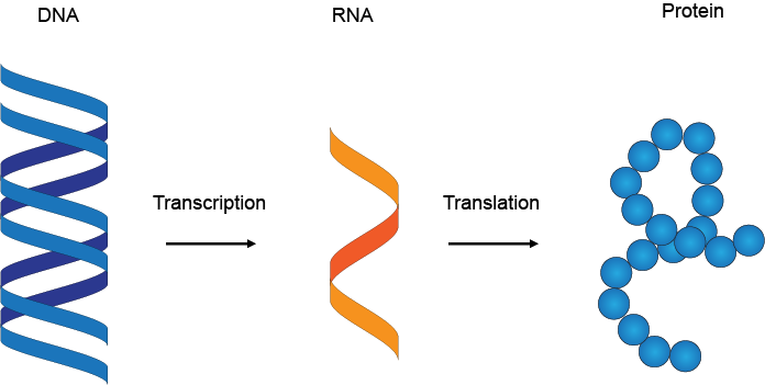
Figure 1: The Central Dogma of Molecular Biology

The current linguistic view of biological sequences focuses on the grammar like structures in gene, RNA molecule or protein. We will give a brief review of the relevant molecular structures and then describe their linguistic analyses using formal grammars.

2.1 The biological structures of gene, RNA molecule and protein

DNA, or deoxyribonucleic acid, is the hereditary material carrying all the genetic information in humans and almost all other organisms. The information in DNA is stored as a code made up of four chemical bases: adenine (A), guanine (G), cytosine (C), and thymine (T). Human DNA consists of about 3 billion bases, and more than 99 percent of those bases are the same in all people. DNA bases pair up with each other, A with T and C with G, to form units called base pairs. Each base is attached to a sugar and a phosphate to form a nucleotide. Nucleotides are further arranged in two long strands that form a spiral called a double helix, which is the basic structure of DNA. The sequence of DNA is denoted by the sequence of bases in the nucleotides (Figure 2).

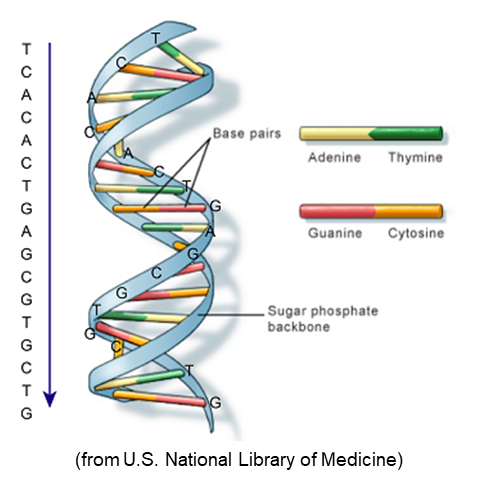
Figure 2: The structure and sequence of DNA

A gene is a fragment of DNA that can be expressed as functional RNA or protein as shown in Figure 3. We can see from the figure that a gene can be transcribe into a message RNA (mRNA) and the mRNA is further translated into a protein which has its specific biological function. This was emphasized in the above mentioned centre dogma. Alternatively, the gene could be transcribed into a non-coding RNA (ncRNA) which won’t be translated into protein, but itself has certain biological functions. This is relatively new discovery after the establishment of the centre dogma. Both the protein and ncRNA also have secondary structure besides the primary structures. Here, by primary structure we refer to the linear sequence and by secondary structure we mean the 2-D patterns often formed in ncRNA and proteins. The most common secondary structures in proteins include $\alpha$-helix or $\beta$-sheet, and for ncRNA we very often see pseudoknots or stem-loops.

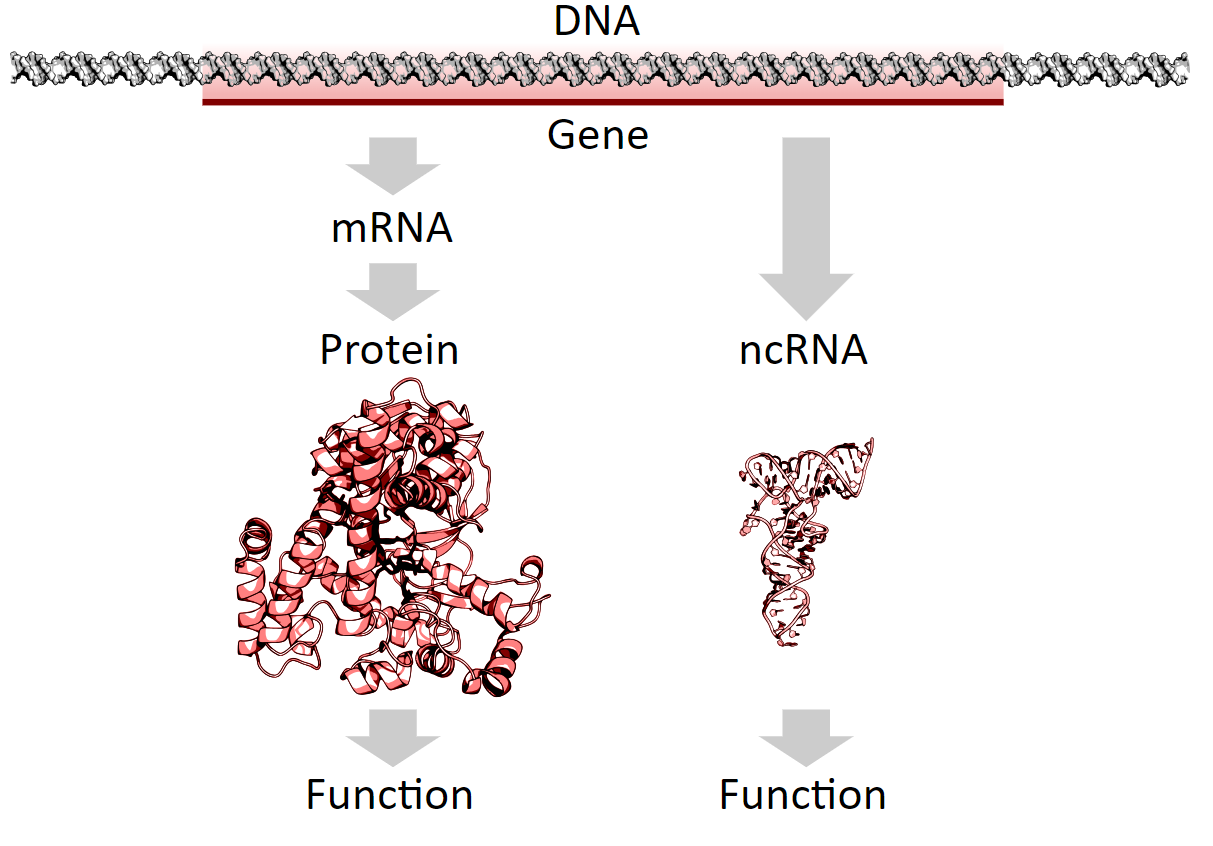
Figure 3: Functional expression of a gene (by Thomas Shafee)

2.2 A brief review of macro-molecular linguistics

We will first describe the gene grammar. A typical eukaryote gene which codes for a protein has the structure shown in Figure 4. Basically, a gene is composed of a Promoter followed with a Transcript, which has it basic parts: the 5’UTR, an Open Reading Frame (ORF) and the 3’UTR. The ORF contains a serials of Exons separated by Introns. UTR stands for untranslated region, and they will be eliminated together with those Introns from the Transcript sequence to form a coding sequence (CDS) which actually codes for the protein sequences (Figure 4).

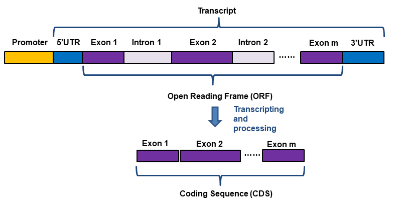
Figure 4: A typical eukaryote gene structure

Such a gene can be viewed as resembling a sentence in having a modular structure, which could be captured by a set of grammar rules as following [Searls, 2002, Searls, 2013]:

Gene →Promoter Transcript
    Transcript →5’UTR ORF 3’UTR
    ORF →Exon Intron ORF |Exon
    Exon →CodingSeq
    Intron →Donor SkippedSeq Acceptor
    Donor →gt
    Acceptor →ag
    CodingSeq →atgaacaca…taa
    SkippedSeq →cccaagc…gca

Note that CodingSeq and SkippedSeq are components like words in a sentence, and we use some random DNA sequences to temporarily represent their existence in the grammar structure but these sequences have no real meanings. Here, we only introduced a simplified gene grammar, and much more elaborated models could be found in [Dong and Searls, 1994, Searls, 1993].

For application, this kind of formal grammar in turn could be used to recognize and predict structures of more genes that were previously unexplored [Dong and Searls, 1994].

Now let us move on to the RNA secondary structure grammars. Unlike DNA molecules, which form double helical structure and the two complementary strands are paired uniformly, the RNA molecules usually contains only one single strand. Nevertheless, RNA molecules often fold themselves into various secondary structures such as hairpin, stem-loop, pseudo-knot, dumb-bell, etc.

Here we present an example of a hairpin in Figure 5. The palindromic RNA sequence “GAUC-GAUC” that gives rise to this hairpin can be generated from the context-free grammar that follows [Searls, 2013]:

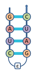
Figure 5: A RNA hairpin

Pair →a Pair u |u Pair a |c Pair g |g Pair c |

More complex RNA secondary structures and their grammar models can be found in [Chiang et al., 2006, Searls and Others, 1999].

Last but not least, we have the protein grammars. As protein has a relatively more complex ”alphabet” which contains 20 amino acids, also the structures of proteins are much more diverse and complicated than that of RNA molecules, there exists no simple grammars for protein so far. Nevertheless, the linguistic properties of protein structure have been extensively studied, and at least for the local structures, several elegant models were established. Those local features include basic secondary components such as - helix or -sheet, as well as many import ligand binding sites.

For example, Figure 6 shows a typical -sheet structure. And the ranked node-rewriting grammar (RNRG) depicted in Figure 7 is able to generate this -sheet [Chiang et al., 2006].

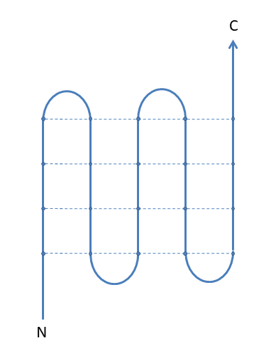
Figure 6: A typical protein secondary structure (-sheet)

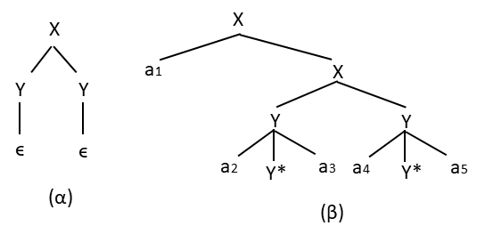
Figure 7: RNRG for -sheet of five strands

In Figure 7, X, Y and Y* represent the non-terminal nodes, while $a_{i}$(i=1..5) and $\epsilon$ refer to terminal nodes (amino acid and empty, respectively). RNRG is essentially tree adjoining grammar (TAG) with multiple foot nodes on elementary trees. In Figure 7, we have 2 elementary trees () and (). The small tree () on the left can be seen as an initial tree, and () on the right is known as auxiliary trees. An initial tree has a root (X here), which stands for the initial node of that tree. On the other hand, an auxiliary tree always has a special foot node marked with a *.

In a regular expression or a context free grammar as mentioned in DNA and RNA grammar, the basic operation is symbol rewriting, i.e. we can replace a symbol on the left hand of an arrow with that on the right hand as stated in the grammar rule. Similarly, in a RNRG the basic operation is node rewriting. When a node X is rewritten with a tree (), the children of X are identified with food nodes of (), matched up according to linear precedence. For example, Figure 8 shows a rewriting of node X using application of tree () from Figure 7 [Chiang et al., 2006].

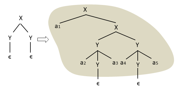
Figure 8: Rewriting of node X

In fact, it was pointed out that many context-free grammars for protein structure could be converted into TAG and related formalisms[Chiang et al., 2006].

Alternatively, a stochastic context free grammar could produce ligand binding sites efficiently[Dyrka and Nebel, 2009].

3 Lambek’s pregroup-based grammar

In 1999, Lambek introduced pregroup as a new computational algebraic approach for analysing the syntactic structure of natural languages [Lambek, 1999].

A pregroup is a mathematical structure respecting the following rules:

1. $(xy)z=x(yz)$ (associativity)

2. $x1=x=1x$ (identity)

3. $x\rightarrow x$ (reflexivity)

4. if $x\rightarrow y$ and $y\rightarrow z$ then $x\rightarrow z$ (transitivity)

5. if $x\rightarrow y$ and $y\rightarrow x$ then $x=y$ (antisymmetry)

6. if $x\rightarrow y$ and $x^{\prime}\rightarrow y^{\prime}$ then $xx^{\prime}\rightarrow yy^{\prime}$ (compatibility)

7. if $x\rightarrow y$ then $uxv\rightarrow uyv$ (substitutivity)

8. $x^{l}x\rightarrow 1$ and $xx^{r}\rightarrow 1$ (contractions)

9. $1\rightarrow xx^{l}$ and $1\rightarrow x^{r}x$ (expansions)

The principle idea of a pregroup grammar is to assign one or more types to each word of a language. These types are elements of a pregroup, and therefore the grammatical status of a sentence (as a string of words) can be calculated from the corresponding types of the words that constitute the sentence. [Lambek, 1999, Lambek, 2008]

In order to construct such a pregroup, one starts by defining a poset (P, →) that consists of a set P of basic types and a partial ordering between them (denoted as ’→’). The basic types represent traditional grammatical terms such as noun, verb, sentence, etc. For any x, y $\in$P, x $\rightarrow$ y means everything of type x is also of type y. Moreover, for each basic type p$\in$P, there exist a left adjoint $p^{l}$ and a right adjoint $p^{r}$ that satisfy rule (8) and (9) above. Also, the adjoints have the following properties[Lambek, 1999]:

• Adjoints are unique

• Adjoints are order reversing: if $p\rightarrow q$ then $q^{r}\rightarrow p^{r}$ and $q^{l}\rightarrow p^{l}$

• The unit is self adjoint: $1^{l}=1=1^{r}$

• Multiplication is self adjoint: $(p\cdot q)^{r}=q^{r}\cdot p^{r}$ and $(p\cdot q)^{l}=q^{l}\cdot p^{l}$

• Opposite adjoints annihilate each other: $(p^{l})^{r}=p=(p^{r})^{l}$

• Same adjoints iterate: $p^{ll}p^{l}\rightarrow 1\rightarrow p^{r}p^{rr}$, $p^{lll}p^{ll}\rightarrow 1\rightarrow p^{rr}p^{rrr}$, …

These adjoints extend basic types to so called simple types, and a string of simple types $x_{1}$…$x_{n}$ with $n\leq 0$ form a compound type. The empty string with $n=0$, is denoted by 1. Furthermore, strings can be multiplies by juxtaposition (cancatenation):

$$(x_{1}...x_{m})(y_{1}...y_{n})=x_{1}...x_{m}y_{1}...y_{n}$$

Finally, with all these constructions and rules, we can calculate the grammar type of a string of words and verify if it is a grammatically sound sentence or not [Lambek, 2008, Lambek, 1999].

This grammar framework is quite different from that of Chomsky, and it was proved to be equivalent to context-free grammars in the Chomsky’s hierarchy [Buszkowski, 2001].

As far as we know, there is no description of macromolecular linguistics using Lambek grammar.

4 The categorical compositional distributional (DisCoCat) model

In 2010, Coecke et al. established a mathematical foundation, named categorical compositional distributional (DisCoCat) model, that could compute the meaning of a sentence from the meanings of its constituent words. The DisCoCat model ingeniously adopts category theory to unify the distributional representations of word meanings in vector spaces with the compositional grammar types of words in a pregroup, and takes advantage of the pregroup algebra to transform the meanings of constituents into a meaning of the whole [Coecke et al., 2010].

The key idea behind DisCoCat model is that both pregroup and vector spaces share the same high level mathematical structure, referred to as a compact closed monoidal category[Grefenstette and Sadrzadeh, 2011].

In category theory, a strict monoidal category $\mathcal{C}$ has the following components and features:

• a collection of objects A, B, C, …

• for each pair of object A, B $\in\mathcal{C}$, a set $\mathcal{C}$(A, B) of morphisms from A to B, each of the morphism is denoted as $f:A\rightarrow B$

• for each $f:A\rightarrow B$ and $g:B\rightarrow C$, we have a composition of morphisms denoted as $g\circ f:A\rightarrow C$

• for each object A $\in\mathcal{C}$, there is an identity morphism $1_{A}:A\rightarrow A$, and for each morphism $f:A\rightarrow B$, we have $f\circ 1_{A}=f=1_{B}\circ f$

• if $f,g,h$ are composable morphisms, we have $(h\circ g)\circ f=h\circ(g\circ f)$ called associativity

• for each pair of object A, B $\in\mathcal{C}$, a composite object $A\otimes B$ called tensor product, which also admits associativity:

  $$(A\otimes B)\otimes C=A\otimes(B\otimes C)$$

• there is a unit object $I$, which satisfies: $I\otimes A=A=A\otimes I$

• the morphism composition and tensor product further satisfy the following rule:

  $$(g_{1}\otimes g_{2})\circ(f_{1}\otimes f_{2})=(g_{1}\circ f_{1})\otimes(g_{2}\circ f_{2})$$

For a monoidal category to become a compact closed one, we have for each object A a pair of objects $A^{l}$ and $A^{r}$ called the left and right adjoints or A, respectively. Also we have morphisms:

$$\eta^{l}:I\rightarrow A\otimes A^{l}\hskip 20.0pt\epsilon^{l}:A^{l}\otimes A\rightarrow I$$

$$\eta^{r}:I\rightarrow A^{r}\otimes A\hskip 20.0pt\epsilon^{r}:A\otimes A^{r}\rightarrow I$$

which satisfy:

$$(1_{A}\otimes\epsilon^{l})\circ(\eta^{l}\otimes 1_{A})=1_{A}\hskip 20.0pt(\epsilon^{r}\otimes 1_{A})\circ(1_{A}\otimes\eta^{r})=1_{A}$$

$$\hskip 8.0pt(\epsilon^{l}\otimes 1_{A^{l}})\circ(1_{A^{l}}\otimes\eta^{l})=1_{A^{l}}\hskip 20.0pt(1_{A^{r}}\otimes\epsilon^{r})\circ(\eta^{r}\otimes 1_{A^{r}})=1_{A^{r}}$$

Once the common underlying structure of vector space and pregroup is identified, one can pair the vectors representing meanings of words with those grammatical types in a pregroup via a strong monoidal functor F that preserve the compact closed structure, and consequently the grammatical reduction of pregroup can be directly transformed into linear maps between the corresponding vectors. If the grammar type of a string of words can be reduced to a sentence, then the corresponding calculation on the vectors would produce the meaning of that sentence also in a vector space.

Concretely, we can perform the following steps in order to compute the meaning of a sentence from a string of words $w_{1}w_{2}...w_{n}$ [Coecke et al., 2010]:

1. assign each word $w_{i}$ a grammar type $p_{i}$

2. assign each word $w_{i}$ a vector space $V_{i}$ and determine its actual vector representation $v_{i}$

3. concatenate the grammar types of words in the string to $p_{1}p_{2}...p_{n}$ and carry out a type reduction upon it using the rules of pregroup algebra, and record the chain of reduction as a morphism

4. apply functor F on the reduction morphism obtained from previous step to get a linear map L, and compute the meaning of the sentence by applying L upon the tensor of vector spaces representing the meaning of corresponding words ($v_{1}\otimes v_{2}\otimes...\otimes v_{n}$)

5 Adopt the DisCoCat model for protein linguisitics

The DisCoCat model combines the distributed representations of word meaning with the grammar types to induce the meaning of a sentence. We propose that equivalent framework could be constructed for proteins. Under such a framework, we treat a protein as a sentence, and the constituent domains or linker regions as words. Consequently, we could obtain the function (meaning) of a protein through combining the vector representation with the grammar type of domains and linkers.

We will layout the process in next sections and will further illustrate it with some examples. Before that, it is obligatory to explain the reasons for us to be optimistic about adopting the DisCoCat model on proteins.

First of all, the modular nature of protein structure has long been noticed. In order to fulfil a large diversity of biological functions, proteins form highly organized 3D structures. According to the protein structure database CATH [Knudsen and Wiuf, 2010] and SCOP [Lo Conte et al., 2000], there are about $1,000\sim 2,000$ different folds (the arrangement of secondary structure) while the number of different proteins is more than 100,000. These structural data provides a strong evidence for protein modularity [Levy, 2017].

Actually, throughout evolution, the process of gene duplication and combination has been the major source of new proteins. The units that are involved in combination, which themselves often kept unchanged, are those so called protein domains (equivalent to ”folds” mentioned above). In the protein research community, a great deal of efforts have been put into classifying those different domains into various families [El-Gebali et al., 2018, Lo Conte et al., 2000, Knudsen and Wiuf, 2010, Mitchell et al., 2018]. In addition, how the different combinations of domains produce new functions in the new proteins has also been studied intensively [Apic et al., 2001, Moore et al., 2008, von Heijne, 2018, Bashton and Chothia, 2007, Bornberg-Bauer et al., 2010, Levy, 2017].

Interestingly enough, an linguistic analogous of the protein producing process to how words combine to form meaningful sentence has been explicitly pointed out in some of the studies for new protein generating [Gimona, 2006, Bashton and Chothia, 2007]. Besides the general observation of a similarity between protein formation and sentence assembly, another property worthwhile a particular mentioning is domain splitting. It was found that in some cases during evolution, two distinct functions previously carried out by a single-domain protein have been separated into discrete functions that individually carried out by two different domains in the new multi-domain protein. This separation of the function domains strongly resemble the generation of discreteness, which is a characteristic feature of the development of natural languages [Senghas et al., 2004, Bashton and Chothia, 2007].

Taken together, the striking similarity between protein and human (natural) languages justifies our attempts to apply the DisCoCat model on proteins. But in order to do that, we need to prepare 2 ingredients: (1) a grammar typing system for proteins that agrees with the Lambek pregroup structure; (2) a distributed representation of protein domains in the vector space. Let us get them ready first.

5.1 Grammar typing the proteins

We start from a hypothetical protein with a representative structure depicted in Figure 9.

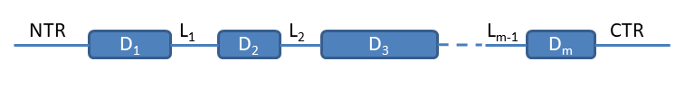
Figure 9: A hypothetical protein structure

The notations in the figure represent:
    NTR: N terminal region
    CTR: C terminal region
    Li (i=1..m-1): the ith Linker region
    Di (i=1..m): the ith Domain

And we introduce the following basic types for these kind of proteins:
    $b$ = binding domain,
    $b_{1}$ = ligand binding domain,
    $b_{2}$ = DNA binding domain,
    $b_{3}$ = RNA binding domain,
    $b_{4}$ = polypeptide binding domain,
    $c$ = catalytic domain,
    $c_{1}$ = oxidoreductase catalytic domain,
    $c_{2}$ = transferase catalytic domain,
    $c_{3}$ = hydrolase catalytic domain,
    $c_{4}$ = lyase catalytic domain,
    $c_{5}$ = isomerase catalytic domain,
    $c_{6}$ = ligase catalytic domain,
    $\bar{c}$ = C-terminal region,
    $i$ = protein-protein interaction domain,
    $l$ = linker region,
    $n$ = N-terminal region,
    $p$ = protein,
    $p_{1}$ = single domain protein,
    $p_{2}$ = multiple domain protein,
    $r$ = regulatory domain,
    $t$ = channel or transporter domain.

Following the Lambek typing protocol [Lambek, 2008], we further introduce a set of postulates here, which enforces a partial order on the previous set of basic types, and through transitivity law other order relations can be derived accordingly.
    $b_{i}\rightarrow b\hskip 10.00002pt(i=1,2,3,4)$;
    $b,i\rightarrow r$;
    $c_{j}\rightarrow c\hskip 10.00002pt(j=1,2,3,4,5,6)$;
    $p_{k}\rightarrow p\hskip 10.00002pt(k=1,2)$;
    $c,t\rightarrow p_{1}$.

5.2 Distributed representation of protein domains

The basic idea behind a distributed representation of words is manifested by this famous quote from John Firth: You should know a word by the company it keeps; i.e., words that appear in similar context will have similar meaning. According to this ”distributional hypothesis”, we can represent the meaning of a word by a n-dimensional vector, in which the orthogonal basis vectors are represented by context words [Firth, 1957, Coecke et al., 2010, Bradley, 2018].

In natural language processing, distributed representations of words in a vector space turned out to be an efficient method [Hinton et al., 1986, Mikolov et al., 2013].

It is desirable to have a distributed representation of protein sequences as well. As vector space is extremely computer friendly, we could then use it as a general-purpose representation in a wide range of bioinformatics problems such as protein family classification, protein structure prediction, protein visualization, etc. Actually, a distributed representation of protein sequences has recently been constructed by a machine learning method called ProtVec [Asgari and Mofrad, 2015]. In general, ProtVec adopted the Word2Vec algorithm from natural language processing but used protein sequences as corpus for training and testing. It turned out that ProtVec could achieve a protein classification accuracy of  93%, which outperformed other existing methods. Moreover, ProtVec appeared to be a powerful approach for protein data visualization.

Here we need to clarify some important details. In ProtVec, the training set is 324,018 protein sequences obtained from Swiss-Prot belonging to 7,027 protein families. The algorithm first split each sequence into 3 different sequences of 3-mers as indicated in Figure 10 [Asgari and Mofrad, 2015].

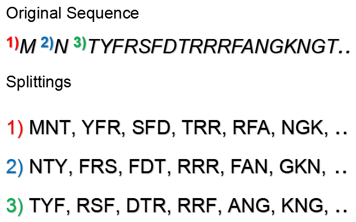
Figure 10: Protein sequence splitting in ProtVec

Each 3-mer is regarded as a ”word”, and a vector of size 100 is assigned to represent this word after a Word2Vec learning process [Mikolov et al., 2013]. Then for each protein sequence, a vector representation is obtained by a summation of the vector representations of the over-lapping 3-mers [Asgari and Mofrad, 2015].

As the sequences of protein domains are highly conserved but those of the domain combinations are not [Gimona, 2006], we conceive that the above mentioned vector representations for protein sequences are reasonable for domains only. Especially, they may not be suitable for those multi-domain proteins. Since the 324,018 protein sequences contain all sorts of reads including both domains and whole proteins, we will therefore only borrow from ProtVec the vector representations of the domains. And we will calculate the vector representation of a whole protein from its individual domains following the DisCoCat model.

Actually, the major significance of adopting the DisCoCat model for a calculation of the protein function exactly lies here. In natural language, the words are highly conserved while the way they compose a sentence is incredibly versatile, therefore we are able to get a vector representation for a word through machine learning algorithm such as Word2Vec, but we couldn’t do the same for a sentence. Similarly, protein domains (”words”) are conserved entities but a combination of those domains into a protein (“sentence”) is highly variable. Thus we need more sophisticated method such as the DisCoCat model.

5.3 Composing the function of proteins

In this section we will illustrate with examples how to compose the function of a protein from its domains. We will first present a toy example with a hypothetical protein sequence and then demonstrate the process with several real proteins.

Suppose we have a protein mockP which has the amino acid sequence and corresponding domain structure shown in Figure 11. Domain1 is a regulatory domain, and Domain2 a catalytic domain. (Note that real proteins will have much longer amino acid sequences than illustrated here)

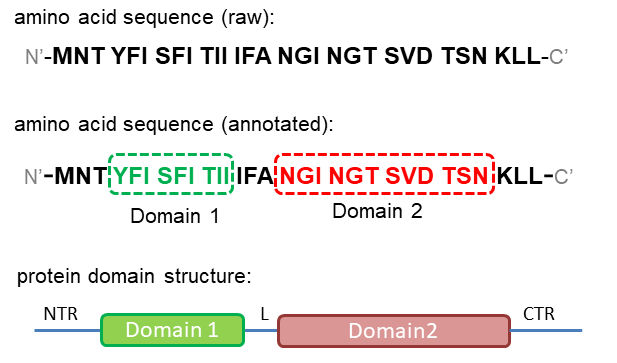
Figure 11: Sequence and domain structure of mockP

The first thing we need to do is to assign types to the individual components (domains) of this protein. We have 5 of them, namely NTR (N terminal region), Domain1 (a regulatory domain), L (Linker), Domain2 (a catalytic domain) and CTR (C terminal region). Previously we tried to involve NTR and CTR in typing, and we found that it only made things unnecessarily complicated. Therefore we choose to ignore NTR or CTR for the time being. Having said that, we have the following types for mockP according to rules in section 5.1:
    Domain1 : $r$;
    L : $r^{r}p_{2}c^{l}$;
    Domain2 : $c$.

By concatenating them together we get the grammar type for the whole protein mockP: $r(r^{r}p_{2}c^{l})c$. Now we could use the contraction rule mentioned in Section 3, and carry out the calculation:

$$\underbracket{r(r^{r}}p_{2}\underbracket{c^{l})c}\hskip 10.00002pt\rightarrow p_{2}$$

The contraction morphism used is $\epsilon_{r}^{r}\cdot 1_{p_{2}}\cdot{\epsilon_{c}}^{l}$.

On the other side, according to Section 4, the tensor product of vector spaces corresponding to the grammar of mockP is: $R\otimes(R\otimes P\otimes C)\otimes C$. Now we translate (lift) the contraction morphism mentioned above to the linear maps in vector spaces and get: $\epsilon_{R}\otimes 1_{P}\otimes\epsilon_{C}$. Next we apply these linear maps to calculate the tensor product of mockP.

Here we will need the vector representations of our domains. As described early in Section 5.2, ProtVec will assign a 100-dimension vector for each domain through training. For the simplicity of this top example, we will assume following vectors for our domains:

$$Domain1=\begin{bmatrix}30\\ 12\\ 9\end{bmatrix}\hskip 30.00005ptL=\begin{bmatrix}1\hskip 10.00002pt0\hskip 10.00002pt0\\ 0\hskip 10.00002pt1\hskip 10.00002pt0\\ 0\hskip 10.00002pt0\hskip 10.00002pt1\end{bmatrix}\hskip 30.00005ptDomain2=\begin{bmatrix}2\\ 4\\ 10\end{bmatrix}$$ (1)

Then we will obtain a vector representation of the meaning (function) of the protein mockP: $\epsilon_{R}\otimes 1_{P}\otimes\epsilon_{C}(Domain1\otimes L\otimes Domain2)$

$$=\begin{bmatrix}30&12&9\end{bmatrix}\begin{bmatrix}1\hskip 10.00002pt0\hskip 10.00002pt0\\ 0\hskip 10.00002pt1\hskip 10.00002pt0\\ 0\hskip 10.00002pt0\hskip 10.00002pt1\end{bmatrix}\begin{bmatrix}2\\ 4\\ 10\end{bmatrix}=\begin{bmatrix}198\end{bmatrix}$$ (2)

Now let us consider some real proteins in the biological world. The proteins we will talk about all belong to the fruit fly Drosophila melanogaster. We study fruit fly instead of human proteins because of the following reasons: (1) fruit fly is the model organism used by the first author in her research; (2) the fruit fly genetics has been extensively studied for over a century, therefore it has the best known genome among all multi-cellular eukaryotes [ModENCODE, 2019, Hales et al., 2015]; (3) at the molecular level, especially when functional domains are concerned, there exists high conservation between fruit fly and human [Hales et al., 2015, Pandey and Nichols, 2011].

As mentioned before, proteins are composed of domains. Many proteins contain only one domain, while others have multiple domains.

Before we get our hands onto the multi-domain proteins, let us first look at a single-domain protein named DAT, which encodes a dopamine transporter in flies. The domain of DAT which fulfills the transporter function is called Sodium:neurotransmitter symporter (Na/ntran_symport). Figure 12 shows the protein domain structure of DAT.

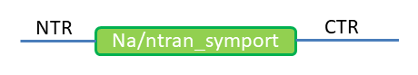
Figure 12: Protein domain structure of DAT

We can simply assign the following type to the domain:

Na/ntran_symport : $t$

We can then follow the typing rules in section 5.1 and do the derivation: $t\rightarrow p_{1}\rightarrow p$, so that we reached the conclusion that this is a grammatically sound protein. As this is a single domain protein, we don’t actually need any calculation. We can simply use the vector representation of the Na/ntran_symport domain for the whole protein. Suppose we obtain it from machine learning algorithms such as implemented in [Asgari and Mofrad, 2015], and let us call it $v_{N}$, we then have $v_{N}$ as the vector space representation of DAT.

The second protein of interest in our examples is FoxP. It was named after its human ortholog FoxP, which is believed to be strongly related to human language [Lai et al., 2001]. FoxP encodes a transcription factor that has the protein domain structure shown in Figure 13.

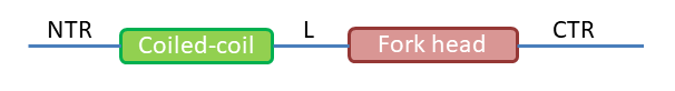
Figure 13: Protein structure of FoxP

According to InterPro [Mitchell et al., 2018], the Coiled-coil domain modulates the dimeric associations of FoxP transcription factors, and the Fork-head domain is a conserved DNA-binding domain. We can assign the following types to the respective domains/regions of the protein FoxP:
    Coiled-coil : $r$;
    L : $r^{r}p_{2}b_{2}^{l}$;
    Fork-head : $b_{2}$.

After concatenating those individual types we will have the grammar type for the FoxP protein as such: $r(r^{r}p_{2}b_{2}^{l})b_{2}$. The corresponding tensor product of vector spaces is: $R\otimes(R\otimes P\otimes B)\otimes B$.

For the grammer type of FoxP, we could use the contraction rule mentioned in Section 3, and carry out the calculation:

$$\underbracket{r(r^{r}}p_{2}\underbracket{b_{2}^{l})b_{2}}\hskip 10.00002pt\rightarrow p_{2}$$

To achieve that, we used the contraction morphism $\epsilon_{r}^{r}\cdot 1_{p_{2}}\cdot{\epsilon_{b_{2}}}^{l}$. We can translate (lift) these morphisms to the linear maps in vector spaces and get: $\epsilon_{R}\otimes 1_{P}\otimes\epsilon_{B}$. These linear maps will be applied to calculate the tensor product of FoxP accordingly. Suppose we get the vector space representations of Coiled-coil domain as $v_{C}$ and that of Fork-head domain as $v_{F}$, and for simplicity we assume the vector representation of the Linker domain is $v_{L}$, then we will obtain a vector representation of the meaning (function) of the protein FoxP as $v_{C}\cdot v_{L}\cdot v_{F}$.

The third gene in our examples is p53. p53 is well known as a tumor suppressor in human, and it also plays important roles in regulating cell death in Drosophila [Levine, 1997, Jin et al., 2000, Sogame et al., 2003]. P53 encodes a transcription factor that has a DNA binding domain and a C-terminal regulatory domain (Figure 14).

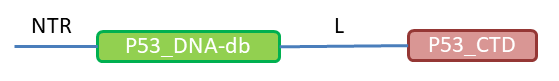
Figure 14: Protein structure of p53

The typing of p53 components are:
    P53_DNA_-db : $b_{2}$;
    L : $b_{2}^{r}p_{2}r^{l}$;
    P53_CTD: $r$.
And accordingly the type of p53 is: $b_{2}(b_{2}^{r}p_{2}r^{l})r$. The corresponding tensor product of vector spaces is: $B\otimes(B\otimes P\otimes R)\otimes R$. Next we use the contraction rules and do the calculation:

$$\underbracket{b_{2}(b_{2}^{r}}p_{2}\underbracket{r^{l})r}\rightarrow p_{2}$$

The contraction morphism used is ${\epsilon_{b_{2}}}^{r}\cdot 1_{p_{2}}\cdot\epsilon_{r}^{l}$. These morphisms can be further lifted to the linear maps in vector spaces: $\epsilon_{B}\otimes 1_{P}\otimes\epsilon_{R}$. And they will be used to calculate the tensor product of p53. If we get the vector space representations of p53_DNA-db domain as $v_{D}$ and that of p53_CTD domain as $v_{C}$, the vector representation of p53 is $v_{D}\cdot v_{L}\cdot v_{C}$.

Let us quickly go through two more examples of proteins with 2 domains – Fruitless (Fru) and Super sex combs (Sxc).

Fru is involved in sex determination and it has a regulatory domain BTB/POZ as well as a DNA binding domain C2H2 (Figure 15) [Ryner et al., 1996].

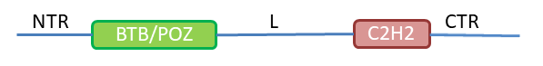
Figure 15: Protein structure of Fruitless

The composing process for Fru is similar to that of FoxP. We first assign the grammar types:
    BTB/POZ : $r$;
    L : $r^{r}p_{2}b_{2}^{l}$;
    C2H2 : $b_{2}$.
The grammar type for Fru therefore is: $r(r^{r}p_{2}b_{2}^{l})b_{2}$. And the tensor product of vector spaces is: $R\otimes(R\otimes P\otimes B)\otimes B$. We then use the contraction rules for calculation:

$$\underbracket{r(r^{r}}p_{2}\underbracket{{b_{2}}^{l})b_{2}}\hskip 10.00002pt\rightarrow p_{2}$$

Similar to FoxP, we also used the contraction morphism $\epsilon_{r}^{r}\cdot 1_{p_{2}}\cdot{\epsilon_{b_{2}}}^{l}$. These morphisms again correspond to the linear maps in vector spaces: $\epsilon_{R}\otimes 1_{P}\otimes\epsilon_{B}$. We can obtain a vector representation of Fru’s function as $v_{BTB}\cdot v_{L}\cdot v_{C2H2}$, given that BTB/POZ is represented by $v_{BTB}$ and C2H2 by $v_{C2H2}$.

Finally, let us look at another protein named Sxc (abbreviation for Super sex combs), a glycosyltransferase involved in polycomb repression, which is essential for controlling the development of fruit fly [Gambetta et al., 2009]. Sxc contains a TPR_repeat domain that mediates its interaction with other proteins, and a OGT/SEC/SPY_C domain carrying the transferase responsibility (Figure 16).

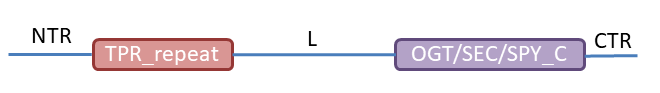
Figure 16: Protein structure of Sxc (Super sex combs)

We can assign the grammar types of the domains of Sxc accordingly:
    TPR_repeat : $i$;
    L : $i^{r}p_{2}c_{2}^{l}$;
    OGT/SEC/SPY_C : $c_{2}$.
The grammar type for Sxc therefore is: $i(i^{r}p_{2}c_{2}^{l})c_{2}$. And the tensor product of vector spaces is: $I\otimes(I\otimes P\otimes C)\otimes C$. We then use the contraction rules for calculation:

$$\underbracket{i(i^{r}}p_{2}\underbracket{{c_{2}}^{l})c_{2}}$$

Here we used the contraction morphism $\epsilon_{i}^{r}\cdot 1_{p_{2}}\cdot{\epsilon_{c_{2}}}^{l}$. These morphisms again corresponds to the linear maps in vector spaces: $\epsilon_{I}\otimes 1_{P}\otimes\epsilon_{C}$. We can obtain a vector representation of Sxc’s function as $v_{T}\cdot v_{L}\cdot v_{O}$, given that TPR_repeat is represented by $v_{T}$ and OGT/SEC/SPY_C by $v_{O}$.

6 Conclusion and future work

In this work, we tried to apply the mathematical model DisCoCat, which was built originally for natural language processing to protein linguistics. Using concrete examples, we demonstrated the detailed process of ”calculating” the meaning or function of a protein from its constituent domains. Therefore we provide a novel way to represent a protein’s function in a vector space.

Our major purpose here is to illustrate the possibility and feasibility of harnessing a state-of-art theory in natural language processing to the language of nature. In order for the method described in the paper to be really useful in practice, two major issues need to be taken care of. First, for the grammar typing of protein domains, we only provided a preliminary option which is far from being complete, therefore it needs to be optimized and improved. Second, the tensor product computation of vector spaces should be stricter than the simplified version here. Particularly, how to assign the vector space representations of different Linker domains would be a centre question to address.

Another aspect worthwhile pursuing after is to embrace the diagrammatic representation as highlighted in the original DisCoCat model [Coecke et al., 2010]. By doing so the process of composing the function of a protein will be much easier to understand intuitively and the calculation itself greatly simplified as well.

References

- [Ajdukiewicz, 1935] Ajdukiewicz, K. (1935). Die syntaktische konnexitat. Studia philosophica, pages 1–27.
- [Apic et al., 2001] Apic, G., Gough, J., and Teichmann, S. A. (2001). Domain combinations in archaeal, eubacterial and eukaryotic proteomes. Journal of Molecular Biology, 310(2):311–325.
- [Asgari and Mofrad, 2015] Asgari, E. and Mofrad, M. R. (2015). Continuous distributed representation of biological sequences for deep proteomics and genomics. PLoS ONE, 10(11):1–15.
- [Bar-Hillel, 1953] Bar-Hillel, Y. (1953). A quasi-arithmetical notation for syntactic description. Language, 29(1):47–58.
- [Bashton and Chothia, 2007] Bashton, M. and Chothia, C. (2007). The Generation of New Protein Functions by the Combination of Domains. Structure, 15(1):85–99.
- [Bornberg-Bauer et al., 2010] Bornberg-Bauer, E., Huylmans, A.-K., and Sikosek, T. (2010). How do new proteins arise? Current Opinion in Structural Biology, 20(3):390–396.
- [Bradley, 2018] Bradley, T.-D. (2018). What is Applied Category Theory?
- [Brendel and Busse, 1984] Brendel, V. and Busse, H. G. (1984). Genome structure described by formal languages. Nucleic Acids Research, 12(5):2561–2568.
- [Buszkowski, 2001] Buszkowski, W. (2001). Lambek grammars based on pregroups. Technical report.
- [Chiang et al., 2006] Chiang, D., Joshi, A. K., and Searls, D. B. (2006). Grammatical Representations of Macromolecular Structure. Journal of Computational Biology, 13(5):1077–1100.
- [Chomsky, 1957] Chomsky, N. (1957). Syntactic structure. Mouton.
- [Coecke et al., 2010] Coecke, B., Sadrzadeh, M., and Clark, S. (2010). Mathematical Foundations for a Compositional Distributional Model of Meaning.
- [Doerfler, 1982] Doerfler, W. (1982). IN SEARCH OF MORE COMPLEX GENETIC CODES-CAN LINGUISTICS BE A GUIDE? Technical report.
- [Dong and Searls, 1994] Dong, S. and Searls, D. B. (1994). Gene structure prediction by linguistic methods.
- [Dyrka and Nebel, 2009] Dyrka, W. and Nebel, J. C. (2009). A stochastic context free grammar based framework for analysis of protein sequences. BMC Bioinformatics, 10:323.
- [El-Gebali et al., 2018] El-Gebali, S., Mistry, J., Bateman, A., Eddy, S. R., Luciani, A., Potter, S. C., Qureshi, M., Richardson, L. J., Salazar, G. A., Smart, A., Sonnhammer, E. L. L., Hirsh, L., Paladin, L., Piovesan, D., Tosatto, S. C. E., and Finn, R. D. (2018). The Pfam protein families database in 2019. Nucleic Acids Research.
- [Firth, 1957] Firth, J. R. (1957). A synopsis of linguistic theory 1930-55. Studies in Linguistic Analysis (special volume of the Philological Society), 1952-59:1–32.
- [Gambetta et al., 2009] Gambetta, M. C., Oktaba, K., and Müller, J. (2009). Essential Role of the Glycosyltransferase Sxc/Ogt in Polycomb Repression. Science, 325(5936):93–96.
- [Gimona, 2006] Gimona, M. (2006). Protein linguistics - A grammar for modular protein assembly? Nature Reviews Molecular Cell Biology, 7(1):68–73.
- [Grefenstette and Sadrzadeh, 2011] Grefenstette, E. and Sadrzadeh, M. (2011). Experimental Support for a Categorical Compositional Distributional Model of Meaning. In Proceedings of the Conference on Empirical Methods in Natural Language Processing, EMNLP ’11, pages 1394–1404, Stroudsburg, PA, USA. Association for Computational Linguistics.
- [Hales et al., 2015] Hales, K. G., Korey, C. A., Larracuente, A. M., and Roberts, D. M. (2015). Genetics on the Fly: A Primer on the Drosophila Model System. Genetics, 201(3):815–42.
- [Hinton et al., 1986] Hinton, G. E., McClelland, J. L., and Rumelhart, D. E. (1986). Distributed Representations. In Rumelhart, D. E., McClelland, J. L., and PDP Research Group, C., editors, Parallel Distributed Processing: Explorations in the Microstructure of Cognition, Vol. 1, pages 77–109. MIT Press, Cambridge, MA, USA.
- [Jin et al., 2000] Jin, S., Martinek, S., Joo, W. S., Wortman, J. R., Mirkovic, N., Sali, A., Yandell, M. D., Pavletich, N. P., Young, M. W., and Levine, A. J. (2000). Identification and characterization of a p53 homologue in Drosophila melanogaster. Proceedings of the National Academy of Sciences of the United States of America, 97(13):7301–6.
- [Knudsen and Wiuf, 2010] Knudsen, M. and Wiuf, C. (2010). The CATH database. Human genomics, 4(3):207–12.
- [Lai et al., 2001] Lai, C. S. L., Fisher, S. E., Hurst, J. A., Vargha-Khadem, F., and Monaco, A. P. (2001). A forkhead-domain gene is mutated in a severe speech and language disorder. Nature, 413(6855):519–523.
- [Lambek, 1958] Lambek, J. (1958). The Mathematics of Sentence Structure. The American Mathematical Monthly, 65(3):154.
- [Lambek, 1968] Lambek, J. (1968). Deductive systems and categories. Theory of Computing Systems, 2(4):287–318.
- [Lambek, 1969] Lambek, J. (1969). Deductive systems and categories II. Standard constructions and closed categories. In Category theory, homology theory and their applications I, pages 76–122. Springer.
- [Lambek, 1972] Lambek, J. (1972). Deductive systems and categories III. Cartesian closed categories, intuitionist propositional calculus, and combinatory logic. In Toposes, algebraic geometry and logic, pages 57–82. Springer.
- [Lambek, 1988] Lambek, J. (1988). Categorial and categorical grammars. In Categorial grammars and natural language structures, pages 297–317. Springer.
- [Lambek, 1999] Lambek, J. (1999). Type Grammar Revisited. Technical report.
- [Lambek, 2008] Lambek, J. (2008). From word to sentence: a computational algebraic approach to grammar. Technical report.
- [Levine, 1997] Levine, A. J. (1997). p53, the cellular gatekeeper for growth and division. Cell, 88(3):323–31.
- [Levy, 2017] Levy, Y. (2017). Protein Assembly and Building Blocks: Beyond the Limits of the LEGO Brick Metaphor.
- [Lo Conte et al., 2000] Lo Conte, L., Ailey, B., Hubbard, T. J., Brenner, S. E., Murzin, A. G., and Chothia, C. (2000). SCOP: a structural classification of proteins database. Nucleic acids research, 28(1):257–9.
- [Mikolov et al., 2013] Mikolov, T., Sutskever, I., Chen, K., Corrado, G., and Dean, J. (2013). Distributed Representations of Words and Phrases and Their Compositionality. In Proceedings of the 26th International Conference on Neural Information Processing Systems - Volume 2, NIPS’13, pages 3111–3119, USA. Curran Associates Inc.
- [Mitchell et al., 2018] Mitchell, A. L., Attwood, T. K., Babbitt, P. C., Blum, M., Bork, P., Bridge, A., Brown, S. D., Chang, H.-Y., El-Gebali, S., Fraser, M. I., Gough, J., Haft, D. R., Huang, H., Letunic, I., Lopez, R., Luciani, A., Madeira, F., Marchler-Bauer, A., Mi, H., Natale, D. A., Necci, M., Nuka, G., Orengo, C., Pandurangan, A. P., Paysan-Lafosse, T., Pesseat, S., Potter, S. C., Qureshi, M. A., Rawlings, N. D., Redaschi, N., Richardson, L. J., Rivoire, C., Salazar, G. A., Sangrador-Vegas, A., Sigrist, C. J. A., Sillitoe, I., Sutton, G. G., Thanki, N., Thomas, P. D., Tosatto, S. C. E., Yong, S.-Y., and Finn, R. D. (2018). InterPro in 2019: improving coverage, classification and access to protein sequence annotations. Nucleic Acids Research.
- [ModENCODE, 2019] ModENCODE (2019). Drosophila as a model organism. http://modencode.sciencemag.org/.
- [Moore et al., 2008] Moore, A. D., Björklund, Å. K., Ekman, D., Bornberg-Bauer, E., and Elofsson, A. (2008). Arrangements in the modular evolution of proteins. Trends in Biochemical Sciences, 33(9):444–451.
- [Pandey and Nichols, 2011] Pandey, U. B. and Nichols, C. D. (2011). Human disease models in Drosophila melanogaster and the role of the fly in therapeutic drug discovery. Pharmacological reviews, 63(2):411–36.
- [Ryner et al., 1996] Ryner, L. C., Goodwin, S. F., Castrillon, D. H., Anand, A., Villella, A., Baker, B. S., Hall, J. C., Taylor, B. J., and Wasserman, S. A. (1996). Control of Male Sexual Behavior and Sexual Orientation in Drosophila by the fruitless Gene. Cell, 87(6):1079–1089.
- [Sciacca et al., 2011] Sciacca, E., Spinella, S., Ienco, D., and Giannini, P. (2011). Annotated Stochastic Context Free Grammars for Analysis and Synthesis of Proteins. pages 77–88. Springer, Berlin, Heidelberg.
- [Searls, 1992] Searls, B. (1992). The Linguistics of DNA. American Scientist, 80(6):579–591.
- [Searls, 1993] Searls, D. B. (1993). The Computational Linguistics of Biological Sequences. In Artificial Intelligence and Molecular Biology, chapter 2, pages 47–121. The MIT Press Classics Series and AAAI press, Cambridge, USA, 1993).
- [Searls, 1997] Searls, D. B. (1997). Linguistic approaches to biological sequences. Bioinformatics, 13(4):333–344.
- [Searls, 2002] Searls, D. B. (2002). The language of genes. TL - 420. Nature, 420 VN -(6912):211–217.
- [Searls, 2013] Searls, D. B. (2013). Review: A primer in macromolecular linguistics. Biopolymers, 99(3):203–217.
- [Searls and Others, 1999] Searls, D. B. and Others (1999). Formal language theory and biological macromolecules. Series in Discrete Mathematics and Theoretical Computer Science, 47:117–140.
- [Senghas et al., 2004] Senghas, A., Kita, S., and Ozyürek, A. (2004). Children Creating Core Properties of Language: Evidence from an Emerging Sign Language in Nicaragua. Science, 305(5691):1779–1782.
- [Sogame et al., 2003] Sogame, N., Kim, M., and Abrams, J. (2003). Drosophila p53 preserves genomic stability by regulating cell death. Proceedings of the National Academy of Sciences (2003) 100(8) 4696-4701.
- [von Heijne, 2018] von Heijne, G. (2018). Protein Evolution and Design. Annual Review of Biochemistry, 87(1):101–103.