A Robust Unscented Transformation for Uncertain Moments

Abstract

This paper proposes a robust version of the unscented transform (UT) for one-dimensional random variables. It is assumed that the moments are not exactly known, but are known to lie in intervals. In this scenario, the moment matching equations are reformulated as a system of polynomial equations and inequalities, and it is proposed to use the Chebychev center of the solution set as a robust UT. This method yields a parametrized polynomial optimization problem, which in spite of being NP-Hard, can be relaxed by some algorithms that are proposed in this paper.

1 Introduction

In numerous problems of statistics and stochastic filtering, one is often interested in calculating the posterior expectation of a continuous random variable $X$ that undergoes a nonlinear transform $f$, viz.:

$$\textrm{E}\left\{f(X)\right\}=\int_{\mathbb{R}}f(\xi)p_{X}(\xi)d\xi.$$ (1)

It is not always possible to have a closed-form expression for this integral in terms of elementary functions: if this integral does not satisfy the hypothesis of Liouville’s theorem (see for instance, Section 12.4 of [1]), then the antiderivative of this integral cannot be expressed in terms of elementary functions. Thus, instead of using analytical methods to calculate (1), in many situations numerical methods must be employed.

A common way to numerically calculate (1) is by using the Monte Carlo integration method [2], which is a stochastic sampling technique: by taking a sufficiently large number of samples of the random variable $X$, one can approximate the probability density function $p_{X}$ and obtain an estimate for (1). However, this method can be very demanding computationally, since it frequently employs several thousands of simulations to obtain the statistics of the final result.

Another way to calculate (1) with less computational burden than Monte Carlo integration method is the technique of Unscented Transform (UT). Originally proposed for the problem of extending the Kalman filter for nonlinear dynamical systems [3], this method has also been applied in several problems of engineering, such as in the analysis of the sensitivity of antennas [4] and in circuit optimization [5].

Different from the Monte Carlo integration method, the UT is a deterministic sampling technique: in place of choosing random points to approximate $p_{X}$, points known as sigma points are deterministically selected to capture the statistics of $p_{X}$. This is accomplished by generating a discrete distribution $p^{\prime}_{X}$ having the same first and second (and possibly higher) moments of $p_{X}$. The mean, covariance and higher moments of the transformed ensemble of sigma points can then be computed as the estimate of the nonlinear transformation $f$ of the original distribution [3], [6]. Thus, at least the first moments of $p_{X}$ must exist and be exactly known. In several circumstances, however, this is not valid: for instance, it may be the case that the distribution does not even have the first moment (one example is the Cauchy distribution [7]). In the case that the moments can be assumed to exist, it is usual that they are not precisely known, but it is still possible to have upper and lower bounds for the exact value of moments from statistical experiments or by the use, for instance, of Chebychev’s inequality [2].

In this paper it is designed a technique for generating sigma points when the exact value of the moments are not known, but upper and lower bounds for the unknown moments are known. In this case, the moment matching equations of UT are no longer just a system of polynomial equations but a system of polynomial equations with polynomial inequalities. Furthermore, since this system can have more than one solution, it is possible to choose a set of sigma points which minimizes a given cost function by formulating the problem as a polynomial optimization problem (POP). Although the solution to this problem is in general computationally infeasible [8], by using Lasserre’s hierarchy of semidefinite programming relaxations one can approximate the solution of the original POP problem by the solution of a computationally feasible convex optimization problem[9, 10].

The main contribution of this paper is the introduction of the concept of UT robustness in the sense of exploiting the upper and lower bounds for moments. A robust UT is proposed in [11] but robustness has different meaning and it is achieved by matching precisely known high order moments. It is important to note that Lasserre’s hierarchy of relaxations was applied in earlier investigations of the moment matching problem [12], but its use was limited to polynomial equations while here polynomial inequalities are also taken into account.

This paper is organized as follow. Some preliminaries for the robust UT are presented in Section 2. The robust UT itself is detailed in Section 3. Details about the computation of robust sigma points is presented in Section 4. The computation of UT transform is presented in Section 5. Finally, the conclusion is presented in Section 7.

2 Unscented Transform

The rationale behind the unscented transformation is that it is easier to calculate a moment for a discrete distribution than a continuous one. In fact, to compute the posterior distribution of a random scalar variable $X$ with distribution $p_{X}$ by a function $f$, one must calculate the integral (1) while, in other hand, if $Z$ is a discrete random variable with $m+1$ atoms $z_{i}$ and distribution $p_{Z}$, one only needs to calculate the sum

$$E\left\{f(Z)\right\}=\sum_{i=1}^{m+1}f(z_{i})p_{Z}(z_{i}).$$ (2)

Henceforth, if it is possible to choose the atoms and their weights of an adequate $p_{Z}$ to approximate $p_{X}$, then the value $E\{f(Z)\}$ would be a good approximation to $E\{f(X)\}$, but with (2) being easier to compute than (1). Thus, the principle behind the UT is to approximate the continuous distribution $p_{X}$ by the discrete distribution $p_{Z}$ by equating the first $m$ moments of these distributions. In other words, the following equations must be satisfied:

$$E\{X^{k}\} =E\{Z^{k}\}$$ (3)

$$=\sum_{i=1}^{m+1}z_{i}^{k}p_{Z}(z_{i}),\ k=1,\ldots,m,$$ (4)

where is supposed the access to $E\{X^{k}\}$ for $k=1,\ldots,m$.

Given $E\{X^{k}\}$ it is always possible to find $z_{i}$ and $p_{Z}(z_{i})$, $i=1,\ldots,m+1$ (which will be called sigma point and its weight, respectively) satisfying (4). In fact, as it will be stated next, there is at least one solution for the equations

$$E\left\{g_{k}(Z)\right\}=E\left\{g_{k}(X)\right\},\ k=1,\ldots,m,$$ (5)

where $g_{k}:\mathbb{R}\rightarrow\mathbb{R}$ are continuous functions, $g_{k}\not\equiv g_{j}$ for $k\neq j$ and from which (4) is a particular case with $g_{k}(x)=x^{k}$. That (5) has at a least one solution is stated next in Theorem 1.

Theorem 1.

Consider that the $m$ moments $E\{g_{k}(X)\}$, $k=1,\ldots,m$, are given. The system (5) in terms of variables $z_{i}$ and $p_{Z}(z_{i})$ has at least one solution with at most $m+1$ sigma points.

Proof.

Since the point $P=\left(E\left\{g_{1}(X)\right\},\ldots,E\left\{g_{m}(X)\right\}\right)$ belongs to the convex hull of the set $G=\left\{\left(g_{1}(x),\ldots,g_{m}(x)\right)\mid x\in\mathbb{R}\right\}$, then Caratheodory’s theorem [14, Theorem 1.3.6] gives that $P$ can be written as a convex combination of at most $m+1$ points in $G$. Thus, one has that there exist $\theta_{i}\geq 0$ and $z_{i}\in\mathbb{R}$ such that

$$E\{g_{k}(X)\}=\sum_{i=1}^{m+1}\theta_{i}g_{k}(z_{i}),\ k=1,\ldots,m$$ (6)

and

$$\sum_{i=1}^{m+1}\theta_{i}=1.$$ (7)

Taking $Z$ to be the discrete random variable with probability distribution given by

$$p_{Z}(k)=\begin{cases}\theta_{i},&\text{if }k=z_{i},\\ 0,&\text{otherwise,}\end{cases}$$

one has that equations (6) and (7) are exactly the equations given by (5). ∎

It is important to note that Theorem 1 only states the existence of sigma points satisfying (5), but it does not give any conclusion about uniqueness. In fact, many solutions are possible, and the choice of an adequate set of sigma points has been investigated thoroughly in the literature [6, 15].

Remark 1.

Specifically for the first moments of $X$ focused in this paper, i.e. the case that $g_{k}(x)=x^{k}$, $k=0,\ldots,m+1$, one can also see (4) as a Gaussian quadrature integration scheme with $p_{X}$ being the weighting function and $z_{i}$ and $\omega_{i}:=p_{Z}(z_{i})$, $i=1,\ldots,m+1$, being respectively the nodes and their weights in the quadrature formula. Thus, depending on the probability density function $p_{X}$, the sigma points can be readily calculated as the roots of an orthogonal polynomial [16, Section 4.6]. For instance, if $p_{X}$ is a normal distribution, then the sigma points are the roots of a Hermite polynomial.

One can note that if the only intention were to find some discrete random variable such that $E\{f(X)\}=E\{f(Z)\}$, it is always possible to find a $Z$ variable with two sigma points. In fact, in Theorem 1, consider $m=1$ and $f=g_{1}$. However, this would imply the knowledge of the function $f$. In the UT reasoning, it is sought a greater number of sigma points in order that the approximation $E\{f(X)\}=E\{f(Z)\}$ be valid for a greater number of functions $f$. In [17] it is shown that the approximation is good for any function $f$ which can be well approximated by its $m$-order Taylor representation.

On top of that, the larger is $m$, the more precise is the approximation for $E\{f(X)\}$: an estimate for the error $\int_{a}^{b}p_{X}(x)f(x)\,dx-\sum_{i=1}^{m}\omega_{i}f(z_{i})$ is given by

$$\frac{f^{(2m)}(\xi)}{(2m)!}\int_{a}^{b}p_{X}(x)h_{m}^{2}(x)\,dx,$$

where $\xi\in\left(a,b\right)\subset\mathbb{R}$ and $h_{m}$ is the associated monic orthogonal polynomial of degree $m$ associated to $p_{X}$ [18, Theorem 3.6.24]. As a matter of fact, the Gauss quadrature computed integral for $E\{f(X)\}$ is exact for all $f(x)$ that are polynomials of degree less or equal than $2m-1$ [18, pp. 172-175].

Since Theorem 1 takes in account generic functions $g_{k}$, one can analyze very general moment settings (for instance, the case of fractional moments is worked in [19]).

Summing up, one can note that the basic assumption for the UT theory until now is that the moments are precisely known. However, this assumption can be too strong in practical situations where the moments are estimated from experiments and then, their values are only known to be in some intervals. In this work, we deal with the scenario of unknown moments and propose to calculate a robust set of sigma-points in the sense of minimizing the worst possible error between this robust choice of sigma-points and the sigma-points computed by using the real values of the moments.

3 Robust UT

To motivate the proposed robust UT consider a normally distributed random variable $X$ with mean $\mu$ and variance $V$. In the case where $\mu$ and $V$ are given and $m=2$, it is known that a set of sigma points are given by [6]

$$\begin{array}[]{ccc}z_{1}&=&\mu-\sqrt{3V},\\ z_{2}&=&\mu,\\ z_{3}&=&\mu+\sqrt{3V},\end{array}$$ (8)

with its weights given respectively by $\omega_{1}=\frac{1}{6}$, $\omega_{2}=\frac{2}{3}$ and $\omega_{3}=\frac{1}{6}$.

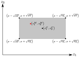
Suppose now that the value of $V$ is not exactly known, but an upper bound $\overline{V}$ and a lower bound $\underline{V}$ for $V$ is known, i.e. $V\in\left[\underline{V},\overline{V}\right]$. A naive approach for choosing the sigma points would be to use the mean value between $\overline{V}$ and $\underline{V}$ for $V$ in (8). In this case, the sigma points $z_{1}$ and $z_{3}$ would be given by

$$z_{1}= z_{1}^{M}\coloneqq\mu-\sqrt{3(\underline{V}+\overline{V})/2},$$

$$z_{3}= z_{3}^{M}\coloneqq\mu+\sqrt{3(\underline{V}+\overline{V})/2},$$

and $z_{2}$, and the weights $\omega_{1}$, $\omega_{2}$ and $\omega_{3}$ unchanged.

As Figure 1 illustrates, this can be a pessimistic choice for the sigma points, since if, for example, the real value of $V$ is in fact nearer of $\bar{V}$, a better choice of sigma points would be nearer to the point $\left(z_{1},z_{3}\right)=\left(\mu-\sqrt{3\overline{V}},\mu+\sqrt{3\overline{V}}\right)$. In fact, as can be seen in Figure 1, a preferable choice for the sigma points would be at the center of the region:

$$z_{1}= z_{1}^{C}\coloneqq\mu-(\sqrt{3}/2)(\sqrt{\underline{V}}+\sqrt{\overline{V}}),$$

$$z_{3}= z_{3}^{C}\coloneqq\mu+(\sqrt{3}/2)(\sqrt{\underline{V}}+\sqrt{\overline{V}}).$$

This choice is precisely the Chebychev center of the set of possibles sigma points given that $V\in\left[\underline{V},\overline{V}\right]$. It has the property of having the minimum worst possible error between the chosen sigma point set and the sigma point set corresponding to the true value of $V$.

Figure 1: Possible choices of sigma points.

Consider now a general scenario where some of the moments are not known, but upper and lower bounds for them are. In this case, the set of possible sigma points and their weights would be in the semialgebraic set $S\subset\mathbb{R}^{2m+2}$ of elements $x=(z_{1},\ldots,z_{m+1},\omega_{1},\ldots,\omega_{m+1})$, defined as solution of the system

$$S:\qquad\begin{array}[]{cccc}\omega_{j}&\geq&0,&j\in\{1,\ldots,m\},\\ \sum_{i=1}^{m+1}\omega_{i}&=&1,\\ \sum_{i=1}^{m+1}z_{i}^{k_{1}}\omega_{i}&=&E\{X^{k_{1}}\},&k_{1}\in\mathcal{K}_{1},\\ \sum_{i=1}^{m+1}z_{i}^{k_{2}}\omega_{i}&\leq&u_{k_{2}},&k_{2}\in\mathcal{K}_{2},\\ \sum_{i=1}^{m+1}z_{i}^{k_{2}}\omega_{i}&\geq&\ell_{k_{2}},&k_{2}\in\mathcal{K}_{2},\end{array}$$ (9)

where $\mathcal{K}_{1}$ (resp. $\mathcal{K}_{2}$) is the set of indexes $k$ for which the $k$-moment is known (resp. unknown), $\mathcal{K}_{1}\cup\mathcal{K}_{2}=\{1,\ldots,m\}$ and $u_{k_{2}}$ and $\ell_{k_{2}}$ are respectively known upper and lower bounds for the $k_{2}$-moment.

Although Theorem 1 guarantees a solution for (9), this solution may not be unique. On that account, there is more than one set of sigma points and corresponding weights, and it is natural to ask which is a good choice of sigma points and weights. Based on the previous example, a so-called robust choice would be the Chebychev center of the semialgebraic set defined by (9) since this choice minimizes the worst possible error between the chosen sigma point set and the sigma point set corresponding to the possible true values of the moments of $X$.

Different from the previous example, however, in this generic scenario it may be the case that an analytic formula to express the sigma points as the function of the moments of the random variable $X$ is not available, and the following optimization problem must be solved to find the Chebychev center:

$$(z_{1}^{C},\ldots,z_{m+1}^{C},\omega_{1}^{C},\ldots,\omega_{m+1}^{C})=\underset{\hat{x}\in\mathbb{R}^{2m+2}}{\arg\min}\ \underset{x\in S}{\max}\|x-\hat{x}\|^{2},$$ (10)

where $S$ is the solution set for (9) and $x=(z_{1},\ldots,z_{m+1},\omega_{1},\ldots,\omega_{m+1})$.

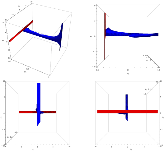
It is important to note that the optimization problem in (10) is not always guaranteed to have a solution, since the set $S$ may not be bounded (if, for example, $\omega_{1}$ is zero, then $z_{1}$ can take any value). Nevertheless, it still makes sense to use the Chebychev center of a large bounded subset of $S$ to try to choose a set of sigma points minimizing the worst possible estimation error. In fact, for any (bounded or unbounded) set $S$, one can take an $\varepsilon>0$ and consider the Chebychev center of the semi-algebraic set $S_{\varepsilon}\subseteq S$ defined as the set of points

$$x=(z_{1},\ldots,z_{m+1},\omega_{1},\ldots,\omega_{m+1})$$

satisfying

$$S_{\varepsilon}:\qquad\begin{array}[]{cccc}\omega_{j}&\geq&\varepsilon,&j\in\{1,\ldots,m\},\\ \sum_{i=1}^{m+1}\omega_{i}&=&1,\\ \sum_{i=1}^{m+1}z_{i}^{k_{1}}\omega_{i}&=&E\{X^{k_{1}}\},&k_{1}\in\mathcal{K}_{1},\\ \sum_{i=1}^{m+1}z_{i}^{k_{2}}\omega_{i}&\leq&u_{k_{2}},&k_{2}\in\mathcal{K}_{2},\\ \sum_{i=1}^{m+1}z_{i}^{k_{2}}\omega_{i}&\geq&\ell_{k_{2}},&k_{2}\in\mathcal{K}_{2}.\end{array}$$ (11)

As $\varepsilon$ decreases, $S_{\varepsilon}$ covers a larger part of $S$. Fig. 2 illustrates how the set $S_{\varepsilon}$ approximates the set $S$ by choosing a sufficiently small $\varepsilon>0$.

While the Chebychev center of $S$ may not exist, the next theorem assures the existence of the Chebychev center of $S_{\varepsilon}$ for any $\varepsilon>0$.

Theorem 2.

If $m\geq 2$ and $\varepsilon>0$, then the optimization problem

$$(z_{1}^{C},\ldots,z_{m+1}^{C},\omega_{1}^{C},\ldots,\omega_{m+1}^{C})=\underset{\hat{x}\in\mathbb{R}^{2m+2}}{\arg\min}\ \underset{x\in S_{\varepsilon}}{\max}\|x-\hat{x}\|^{2},$$ (12)

has a solution.

Proof.

It suffices to prove that the set $S_{\varepsilon}$ is bounded. The variables $\omega_{i}$, $i=1,\ldots,m+1$ are all inside the $m+1$ dimensional simplex and thus bounded. Since

$$\sum_{i=1}^{m+1}z_{i}^{2}\omega_{i}\leq u_{2},$$

and $\omega_{i}>0$, it is impossible for any variable $z_{i}$ to grow without bound. ∎

Remark 2.

It is interesting to note that alternatively, instead of the compact (closed and bounded) set $S_{\varepsilon}$ one could consider the set $\hat{S}$ defined as the set $S$ up to the first inequalities replaced by a strict inequality (that is, $\omega_{j}\geq 0$ is replaced by $\omega_{j}>0$, $j\in\{1,\ldots,m\}$). This set is indeed bounded as $S_{\varepsilon}$. However, strict inequalities are in general not well-handled by numeric solvers.

Figure 2: The regions $S\setminus S_{\varepsilon}$ (red) and $S_{\varepsilon}$ (blue) are plotted in various viewpoints to illustrate the approximation of the semi-algebraic set $S$ by $S_{\varepsilon}$ with $\varepsilon=0.01$, $m=1$, $\mathcal{K}_{1}=\emptyset$, $\mathcal{K}_{2}=\{1,2\}$, $\ell_{1}=\ell_{2}=0$ and $u_{1}=u_{2}=1$. Only $\omega_{1}$, $z_{1}$ and $z_{2}$ are exhibited in the graphic, since $\omega_{2}=1-\omega_{1}$.

The inner maximization problems of (10) and (12) are polynomial optimization problems (POP). Such problems are ubiquitous and are encountered in several fields [21], such as: finance [22, 23, 24], robust and nonlinear control [25, 26], signal processing [27, 28], quantum physics [29] and materials science [30]. It is known that this problem is NP-Hard in general [8], but despite this, it is possible to approximate a POP by convex optimization problems which are computationally feasible using Lasserre’s hierarchy of semidefinite programming relaxations [9, 10]. In fact, by using the GloptiPoly 3 package [31] or the SparsePOP package [32] for MATLAB, or ncpol2sdpa library [33] for Python, these relaxations can be easily implemented and enables the user to transparently construct an increasing sequence of convex LMI relaxations whose optima are guaranteed to converge monotonically to the global optimum of the original non-convex global optimization problem [26]. Moreover, it is possible to numerically certify the global optimality of the problem.

A direct approach to solve (10) would be to use the mentioned Lasserre’s hierarchy to solve the inner maximization problem for a fixed $\hat{x}=\hat{x}_{0}$ and a local optimization algorithm to search which $\hat{x}_{0}$ minimizes (10). This however, besides being a hard numeric problem, would not guarantee a good approximation to the real value of the Chebychev center. In the next section alternative ways to compute (10) with different trade-off between precision of the result and speed of algorithm are proposed.

4 Computation of robust sigma points

4.1 Computation of an outer box to approximate the Chebychev center

The first proposed approach to find an approximate solution to (12) is to compute an outer-bounding box $B$ of $S_{\varepsilon}$ and approximate the Chebychev center of $S_{\varepsilon}$ by the Chebychev center of $B$. By Theorem 2, for $m\geq 2$ the constraint set $S_{\varepsilon}$ is bounded. Thus, each one of the following polynomial optimization problems on $x=(x_{1},\ldots,x_{2m})\in S_{\varepsilon}$ has solution

$$\underline{z}_{i} =\arg\min_{x\in\mathbb{R}^{2m+2}}x_{i}\text{ s.t. }x\in S_{\varepsilon},\ i=1,\ldots,m+1,$$

$$\underline{\omega}_{i} =\arg\min_{x\in\mathbb{R}^{2m+2}}x_{i+m+1}\text{ s.t. }x\in S_{\varepsilon},\ i=1,\ldots,m+1,$$

$$\overline{z}_{i} =\arg\max_{x\in\mathbb{R}^{2m+2}}x_{i}\text{ s.t. }x\in S_{\varepsilon},\ i=1,\ldots,m+1,$$

$$\overline{\omega}_{i} =\arg\max_{x\in\mathbb{R}^{2m+2}}x_{i+m+1}\text{ s.t. }x\in S_{\varepsilon},\ i=1,\ldots,m+1,$$ (13)

and can be used to construct an outer box

$$B=\{(z_{1},\ldots,z_{m+1},\omega_{1},\ldots,\omega_{m+1})\in\mathbb{R}^{2m+2}:\underline{z}_{i}\leq z_{i}\leq\overline{z}_{i},$$

$$\underline{\omega}_{i}\leq\omega_{i}\leq\overline{\omega}_{i},i=1,\ldots,m+1\}$$

such that $S_{\varepsilon}\subset B$. The next theorem gives an estimate of the error of the outer-bounding box approximation.

Theorem 3.

Let $c_{B}$ be the center of Chebychev of $B$ and let $c_{S}$ be the center of Chebychev of $S_{\varepsilon}$. If $d\coloneqq\|c_{B}-c_{S}\|$ is the defined as the distance between the centers of Chebychev, then

$$d\leq\frac{\textrm{diam}(B)}{2},$$

where $\textrm{diam}(B)$ is the diameter of $B$, that is, the least upper bound of the set of all distances between pairs of points in $B$.

Proof.

Suppose that $d>\textrm{diam}(B)/2$. Thus $c_{S}\not\in B$, and since $c_{S}$ is the center of Chebychev of $S_{\varepsilon}$, one has that $c_{S}$ is in the convex hull of $S_{\varepsilon}$. But this implies that $c_{S}$ is in $B$, and the result follows by contradiction. ∎

4.2 Polynomial optimization program to compute minimum enclosing ball

Another approximate solution to problem (12) can be found by using the two-stage approach of [34]. Since the Chebychev center of $S_{\varepsilon}$ is always inside of the outer box $B$ computed in Section 4.1, problem (10) is equivalent to

$$(z_{1}^{C},\ldots,z_{m+1}^{C},\omega_{1}^{C},\ldots,\omega_{m+1}^{C})=\underset{\hat{x}\in B}{\arg\min}\ \underset{x\in S_{\varepsilon}}{\max}\|x-\hat{x}\|^{2}.$$ (14)

In the first stage, the inner optimization problem of (14), namely,

$$J(\hat{x})\coloneqq\max_{x\in S_{\varepsilon}}\|x-\hat{x}\|^{2},$$

is approximated by a polynomial function $\tilde{J}_{\tau}(\hat{x})$ of degree $2\tau$ using the semidefinite optimization program outlined in [34]. Then, in the second stage, the outer minimization problem is replaced with the polynomial optimization problem

$$(z_{1}^{C},\ldots,z_{m+1}^{C},\omega_{1}^{C},\ldots,\omega_{m+1}^{C})=\underset{\hat{x}\in B}{\arg\min}\ \tilde{J}_{\tau}(\hat{x}),$$ (15)

which can be solved using the Lasserre’s hierarchy. As the degree $2\tau$ of the approximation polynomial increases, the solution of problem (15) converges to the solution of problem (14) in the sense of [34]. Alternatively, problem (12) can be shown to be equivalent to the following polynomial optimization problem:

$$\begin{array}[]{cc}\min_{\hat{x},r}r&\text{ s.t. }\|x-\hat{x}\|^{2}\leq r,\\ &x\in S_{\varepsilon},\,\hat{x}\in B,\end{array}$$ (16)

where $\hat{x}$ is the Chebychev center of $S_{\varepsilon}$. In other words, the Chebychev center is the center of the radius of the minimum volume ball that encloses $S_{\varepsilon}$.

Remark 3.

It is interesting to note that if the gap between $\ell_{i}$ and $u_{i}$ is not large enough, the resulting semi-definite programs from relaxing the polynomial optimization problems (13) and (16) can be numerically unstable. In this case, however, one may use the naive approach of computing sigma points by using the arithmetic mean of the moments without loss, since the difference between the real Chebychev center and the point computed by this method would be not so great due to the small difference between the upper and lower bounds of the moments.

5 Computation of UT transform

Suppose that $x_{CB}\coloneqq(z_{1}^{C},\ldots,z_{m+1}^{C},\omega_{1}^{C},\ldots,\omega_{m+1}^{C})$ is the Chebychev center of $S$ computed by one of the methods of Section 4. Based on (2), define the function

$$UT_{f}(z_{1},\ldots,z_{m+1},w_{1},\ldots,w_{m+1})\coloneqq\sum_{i=1}^{m+1}w_{i}f(z_{i}).$$

As discussed above, $UT_{f}$ is a good approximation for $E\{f(X)\}$ for a sufficiently large $m$. While it is true that $x_{CB}$ approximates of the center of Chebychev of $S$, one also wish to know if $UT_{f}(x_{CB})$ is near to the Chebychev center of $UT_{f}(S)$ (that is, the image of the set $S$ by the function $UT_{f}$). A class of functions $f$ such that $UT_{f}(x_{CB})$ is near the Chebychev center of $UT_{f}(S)$ is given by the functions such that the solution of the following optimization problem

$$\min\,D\ \text{s.t.\ } (1-D)\|x-y\|\leq\|UT_{f}(x)-UT_{f}(y)\|$$ (17)

$$\leq(1+D)\|x-y\|,$$

$$x,y\in S$$

is sufficiently small. If these values are sufficiently small, the function $UT_{f}$ is a low-distortion geometric embedding [35], and this implies that $UT_{f}(x_{CB})$ is near the Chebychev center of $UT_{f}(S)$. Finally, to compute (17), one can estimate a solution for (17) by uniformly sampling random values $(x_{i},y_{i})$ of $S$ and computing $\max\,D_{i}$, where

$$D_{i}\coloneqq\min\,D\ \text{s.t.\ } (1-D)\|x_{i}-y_{i}\|\leq\|UT_{f}(x_{i})-UT_{f}(y_{i})\|$$ (18)

$$\leq(1+D)\|x_{i}-y_{i}\|.$$

6 Numerical experiments

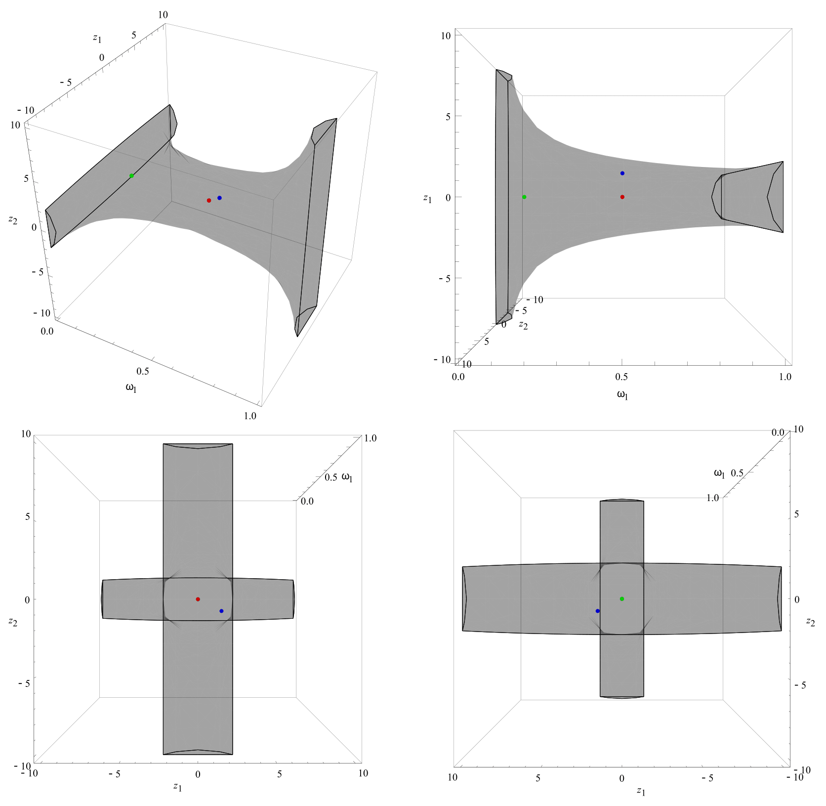
In this example, the computation of Chebychev center using the methods proposed in this paper will be illustrated. Consider that one desires to compute $2$ sigma points in a scenario where the values of the first and second moment are not precisely known, but it is known that $E\{X\}\in[0,1]$ and that $E\{X^{2}\}\in[0,1]$. In this case, one has (9) with $m=1$, $\mathcal{K}_{1}=\emptyset$, $\mathcal{K}_{2}=\{1,2\}$, and $\ell_{1}=-3$ and $u_{1}=4$, and $\ell_{2}=0$ and $u_{2}=5$.

Naive method: For fixed values of $E\{X\}=\mu$ and $E\{X^{2}\}=V$, one can compute a point inside the set $S$ by using the canonical formula

$$\begin{array}[]{c}\omega_{1}=0.5,\ \omega_{2}=0.5,\\ z_{1}=\mu+\sqrt{V-\mu^{2}},\ z_{2}=\mu-\sqrt{V-\mu^{2}}.\end{array}$$ (19)

A naive choice of sigma points would be the use of the arithmetic mean of the lower and upper bounds for the moments in (19). Using (19) with $\mu=\frac{1}{2}(\ell_{1}+u_{1})=0.5$ and $V=\frac{1}{2}(\ell_{2}+u_{2})=2.5$ results in the sigma points $z_{1}=2$, $z_{2}=-1$ with weights given by $w_{1}=0.5$ and $w_{2}=0.5$.

Method 1: By using the method proposed in Section 4.1 it is possible to compute an outer-bounding box approximation to the semi-algebraic set $S_{\varepsilon}$. Using $\varepsilon=0.01$, the computation of an approximate point of the Chebychev center using outer-bounding box approximation results in the sigma points $z_{1}=0$, $z_{2}=0$ with weights respectively given by $w_{1}=0.5$ and $w_{2}=0.5$.

Method 2: Finally, by computing a point using the method proposed in Section 4.2 with $\varepsilon=0.01$ results in the sigma points $z_{1}=-0.0001$, $z_{2}=0.0001$ with weights respectively given by $w_{1}=0.1$ and $w_{2}=0.9$.

In both Method 1 and 2, the MATLAB toolbox Gloptipoly 3 was used to relax the polynomial optimization problems (13) and (16). A relaxation order of $2$ was used and the global optimality of the problems was numerically certified by Gloptipoly3. Moreover, higher relaxation orders could not be used, since using bigger relaxation orders results in semi-definite programs with a large number of variables and constraints, and thus yields an unstable numeric problem.

Figure 3 illustrates the semi-algebraic variety $S_{\varepsilon}$ and the coordinates of the sigma points calculated by the three methods. It can be seen by Figure 3 that the point computed by using the outer-bounding box approximation is the best approximation to the real Chebychev center of the variety. Moreover, it is important to note that the point calculated by Method 2 is very far from the real Chebychev center of the set $S_{\varepsilon}$. This is due to the semi-definite relaxation of (16) being far from the exact solution. In principle, one can increase the relaxation, but this can lead to an unstable numeric problem, which global optimality cannot be more certified.

Figure 3: Semi-algebraic variety $S_{\varepsilon}$ with $\varepsilon=0.01$, $m=1$, $\mathcal{K}_{1}=\emptyset$, $\mathcal{K}_{2}=\{1,2\}$, $\ell_{1}=-3$, $u_{1}=4$, $\ell_{2}=0$ and $u_{2}=5$. The blue point is the coordinates of the sigma-point obtained by the naive method, the red point is the coordinates of the sigma-point obtained by the outer-bounding box approximation, and the green point is obtained by solving the polynomial optimization problem (16) directly. Only $\omega_{1}$, $z_{1}$ and $z_{2}$ are illustrated in the graphic, since $\omega_{2}=1-\omega_{1}$.

Finally, to illustrate the robustness of the computed point, $100$ random samples from $E\{X\}$ and $E\{X^{2}\}$ are respectively draw from the uniform distributions $U(\ell_{1},u_{1})$ and $U(\ell_{2},u_{2})$. Solving (18) for $f(x)=\sin(x)$ with $500$ samples gives an estimate for $D$ of $0.9956$, and the posterior expectation in (1) is approximated as

$$\textrm{E}\left\{\sin(X)\right\}\approx\omega_{1}\sin(z_{1})+\omega_{2}\sin(z_{2}),$$

where $\omega_{1}$, $\omega_{2}$, $z_{1}$ and $z_{2}$ are computed according to the above methods. The mean error $\left|E\{\sin(X)\}-\sum_{i=1}^{2}\omega_{i}\sin(z_{i})\right|$ by the naive method is $0.0339$, while by Method 1 is $3.6932\cdot 10^{-6}$ and by Method 2 is $1.2085\cdot 10^{-4}$.

7 Conclusion

In this paper, it was proposed a way to devise a robust unscented transform by the computation of the Chebychev center of the semialgebraic set defined by the possible choices of sigma points and its weights. Although, in general, this problem is NP-Hard, some methods are proposed in this paper to approximate the solution of the original problem by convex optimization problems. Further works intend to generalize the present work to higher dimensions, as this could enable novel filter designs for multivariate dynamical systems. Another possible extension to this work is to consider adjustments of the proposed algorithm to work with confidence bounds for the moments instead of absolute upper and lower bounds, since the former is more common to be used on interval estimation techniques, such as the bootstrapping method.

Finally, one limitation of the method is that a great number of sigma points can lead to a numerically unstable relaxation of the polynomial optimization problems. Nevertheless, recent advances in polynomial optimization techniques such as novel relaxation hierarchies based on linear programming [36] could help to scale the presented approaches to a higher number of sigma points.

References

- [1] K. O. Geddes, S. R. Czapor, G. Labahn, Algorithms for Computer Algebra, Kluwer Academic Publishers, 1992.
- [2] A. Papoulis, S. U. Pillai, Probability, Random Variables, and Stochastic Processes, McGraw-Hill, New York, 2002.
- [3] S. J. Julier, J. K. Uhlmann, H. F. Durrant-Whyte, A new approach for filtering nonlinear systems, in: Proceedings of the 1995 American Control Conference, Vol. 3, 1995, pp. 1628–1632.
- [4] L. R. A. X. de Menezes, A. J. M. Soares, F. C. Silva, M. A. B. Terada, D. Correia, A new procedure for assessing the sensitivity of antennas using the unscented transform, IEEE Transactions on Antennas and Propagation 58 (3) (2010) 988–993.
- [5] M. L. Carneiro, P. H. P. de Carvalho, N. Deltimple, L. d. C. Brito, L. R. A. X. de Menezes, E. Kerherve, S. G. de Araujo, A. S. Rocira, Doherty amplifier optimization using robust genetic algorithm and unscented transform, in: Proceedings of the 9th IEEE International conference on New Circuits and Systems Conference, IEEE, 2011, pp. 77–80.
- [6] H. M. T. Menegaz, J. Y. Ishihara, G. A. Borges, A. N. Vargas, A systematization of the unscented Kalman filter theory, IEEE Transactions on Automatic Control 60 (10) (2015) 2583–2598.
- [7] K. Krishnamoorthy, Handbook of Statistical Distributions with Applications, CRC Press, 2010.
- [8] K. G. Murty, S. N. Kabadi, Some NP-complete problems in quadratic and nonlinear programming, Mathematical programming 39 (2) (1987) 117–129.
- [9] J. B. Lasserre, Global optimization with polynomials and the problem of moments, SIAM Journal on Optimization 11 (3) (2001) 796–817.
- [10] J. B. Lasserre, Moments, Positive Polynomials and Their Applications, Imperial College Press optimization series, Imperial College Press, Singapore, 2009.
- [11] J. R. Van Zandt, A more robust unscented transform, in: International symposium on optical science and technology, International Society for Optics and Photonics, 2001, pp. 371–380.
- [12] S. Mehrotra, D. Papp, Generating moment matching scenarios using optimization techniques, SIAM Journal on Optimization 23 (2) (2013) 963–999.
- [13] H. Dette, W. J. Studden, The Theory of Canonical Moments with Applications in Statistics, Probability, and Analysis, Vol. 338, John Wiley & Sons, 1997.
- [14] J.-B. Hiriart-Urruty, C. Lemaréchal, Fundamentals of Convex Analysis, Grundlehren Text Editions, Springer, Germany, 2001.
- [15] R. Radhakrishnan, A. Yadav, P. Date, S. Bhaumik, A new method for generating sigma points and weights for nonlinear filtering, IEEE Control Systems Letters 2 (3) (2018) 519–524.
- [16] W. H. Press, S. A. Teukolsky, W. T. Vetterling, B. P. Flannery, Numerical Recipes: The Art of Scientific Computing, 3rd Edition, Cambridge University Press, New York, 2007.
- [17] S. J. Julier, J. K. Uhlmann, Unscented filtering and nonlinear estimation, Proceedings of the IEEE 92 (3) (2004) 401–422.
- [18] J. Stoer, R. Bulirsch, Introduction to Numerical Analysis, Texts in Applied Mathematics, Springer, New York, 2002.
- [19] R. Caballero-Aguila, A. Hermoso-Carazo, J. Linares-Pérez, Extended and unscented filtering algorithms in nonlinear fractional order systems with uncertain observations, Applied Mathematical Sciences 6 (30) (2012) 1471–1486.
- [20] S. Boyd, L. Vandenberghe, Convex Optimization, Cambridge University Press, Cambridge, 2004.
- [21] Z. Li, S. He, S. Zhang, Approximation Methods for Polynomial Optimization: Models, Algorithms, and Applications, Springer Briefs in Optimization, Springer, New York, 2012.
- [22] H. Markowitz, Portfolio selection, The journal of finance 7 (1) (1952) 77–91.
- [23] E. Jondeau, M. Rockinger, Optimal portfolio allocation under higher moments, European Financial Management 12 (1) (2006) 29–55.
- [24] P. M. Kleniati, P. Parpas, B. Rustem, Partitioning procedure for polynomial optimization: Application to portfolio decisions with higher order moments, Tech. Rep. WPS-023, COMISEF Working Papers Series (2009).
- [25] A. P. Roberts, M. M. Newmann, Polynomial optimization of stochastic feedback control for stable plants, IMA Journal of Mathematical Control and Information 5 (3) (1988) 243–257.
- [26] D. Henrion, J.-B. Lasserre, Solving nonconvex optimization problems, Control Systems, IEEE 24 (3) (2004) 72–83.
- [27] B. Mariere, Z.-Q. Luo, T. N. Davidson, Blind constant modulus equalization via convex optimization, Signal Processing, IEEE Transactions on 51 (3) (2003) 805–818.
- [28] L. Qi, K. L. Teo, Multivariate polynomial minimization and its application in signal processing, Journal of Global Optimization 26 (4) (2003) 419–433.
- [29] G. Dahl, J. M. Leinaas, J. Myrheim, E. Ovrum, A tensor product matrix approximation problem in quantum physics, Linear algebra and its applications 420 (2) (2007) 711–725.
- [30] S. Soare, J. W. Yoon, O. Cazacu, On the use of homogeneous polynomials to develop anisotropic yield functions with applications to sheet forming, International Journal of Plasticity 24 (6) (2008) 915–944.
- [31] D. Henrion, J.-B. Lasserre, J. Löfberg, GloptiPoly 3: moments, optimization and semidefinite programming, Optimization Methods & Software 24 (4-5) (2009) 761–779.
- [32] H. Waki, S. Kim, M. Kojima, M. Muramatsu, H. Sugimoto, Algorithm 883: SparsePop—a sparse semidefinite programming relaxation of polynomial optimization problems, ACM Transactions on Mathematical Software 35 (2) (2008) 15.
- [33] P. Wittek, Algorithm 950: Ncpol2sdpa–sparse semidefinite programming relaxations for polynomial optimization problems of noncommuting variables, ACM Transactions on Mathematical Software (TOMS) 41 (3) (2015) 21.
- [34] V. Cerone, J. B. Lasserre, D. Piga, D. Regruto, A unified framework for solving a general class of conditional and robust set-membership estimation problems, IEEE Transactions on Automatic Control 59 (11) (2014) 2897–2909.
- [35] P. Indyk, Algorithmic applications of low-distortion geometric embeddings, in: Proceedings of 42nd IEEE Symposium on Foundations of Computer Science, 2001, pp. 10–33.
- [36] A. A. Ahmadi, A. Majumdar, DSOS and SDSOS optimization: more tractable alternatives to sum of squares and semidefinite optimization, arXiv preprint arXiv:1706.02586.