Adversarial attacks hidden in plain sight

Abstract

Convolutional neural networks have been used to achieve a string of successes during recent years, but their lack of interpretability remains a serious issue. Adversarial examples are designed to deliberately fool neural networks into making any desired incorrect classification, potentially with very high certainty. Several defensive approaches increase robustness against adversarial attacks, demanding attacks of greater magnitude, which lead to visible artifacts. By considering human visual perception, we compose a technique that allows to hide such adversarial attacks in regions of high complexity, such that they are imperceptible even to an astute observer. We carry out a user study on classifying adversarially modified images to validate the perceptual quality of our approach and find significant evidence for its concealment with regards to human visual perception.

1 Introduction

(a) original input

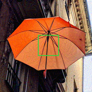
(b) modified input, BIM

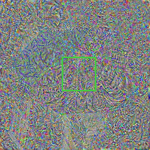
(c) perturbation, BIM

(d) original input (enlarged)

(e) modified input, BIM) (enlarged)

(f) perturbation, BIM) (enlarged)

(g) original input

(h) modified input, EbIM

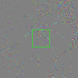
(i) perturbation, EbIM

(j) original input (enlarged)

(k) modified input, EbIM (enlarged)

(l) perturbation, EbIM (enlarged)

Figure 1: Two adversarial attacks carried out using the Basic Iterative Method (first two rows) and our Entropy-based Iterative Method (last two rows). The original image (a) (and (g)) is correctly classified as umbrella but the modified images (b) and (h) are classified as slug with a certainty greater than $99\text{\,}\mathrm{\char 37\relax}$. Note the visible artifacts caused by the perturbation (c), shown here with maximized contrast. The perturbation (i) does not lead to such artifacts. (d), (e), (f), (j), (k), and (l) are enlarged versions of the marked regions in (a), (b), (c), (g), (h), and (i), respectively.

The use of convolutional neural networks has led to tremendous achievements since [1] presented AlexNet in 2012. Despite efforts to understand the inner workings of such neural networks, they mostly remain black boxes that are hard to interpret or explain. The issue was exaggerated in 2013 when [2] showed that “adversarial examples” – images perturbed in such a way that they fool a neural network – prove that neural networks do not simply generalize correctly the way one might naïvely expect. Typically, such adversarial attacks change an input only slightly, but in an adversarial manner, such that humans do not regard the difference of the inputs relevant, but machines do. There are various types of attacks, such as one pixel attacks, attacks that work in the physical world, and attacks that produce inputs fooling several different neural networks without explicit knowledge of those networks [3, 4, 5].

Adversarial attacks are not strictly limited to convolutional neural networks. Even the simplest binary classifier partitions the entire input space into labeled regions, and where there are no training samples close by, the respective label can only be nonsensical with regards to the training data, in particular near decision boundaries. One explanation of the “problem” that convolutional neural networks have is that they perform extraordinarily well in high-dimensional settings, where the training data only covers a very thin manifold, leaving a lot of “empty space” with ragged class regions. This creates a lot of room for an attacker to modify an input sample and move it away from the manifold on which the network can make meaningful predictions, into regions with nonsensical labels. Due to this, even adversarial attacks that simply blur an image, without any specific target, can be successful [6]. There are further attempts at explaining the origin of the phenomenon of adversarial examples, but so far, no conclusive consensus has been established [7, 8, 9, 10].

A number of defenses against adversarial attacks have been put forward, such as defensive distillation of trained networks [11], adversarial training [12], specific regularization [9], and statistical detection [13, 14, 15, 16]. However, no defense succeeds in universally preventing adversarial attacks [17, 18], and it is possible that the existence of such attacks is inherent in high-dimensional learning problems [6]. Still, some of these defenses do result in more robust networks, where an adversary needs to apply larger modifications to inputs in order to successfully create adversarial examples, which begs the question how robust a network can become and whether robustness is a property that needs to be balanced with other desirable properties, such as the ability to generalize well [19] or a reasonable complexity of the network [20].

Strictly speaking, it is not entirely clear what defines an adversarial example as opposed to an incorrectly classified sample. Adversarial attacks are devised to change a given input minimally such that it is classified incorrectly – in the eyes of a human. While astonishing parallels between human visual information processing and deep learning exist, as highlighted e. g. by [21, 22], they disagree when presented with an adversarial example. Experimental evidence has indicated that specific types of adversarial attacks can be constructed that also deteriorate the decisions of humans, when they are allowed only limited time for their decision making [23]. Still, human vision relies on a number of fundamentally different principles when compared to deep neural networks: while machines process image information in parallel, humans actively explore scenes via saccadic moves, displaying unrivaled abilities for structure perception and grouping in visual scenes as formalized e. g. in the form of the Gestalt laws [24, 25, 26, 27]. As a consequence, some attacks are perceptible by humans, as displayed in Figure 1. Here, humans can detect a clear difference between the original image and the modified one; in particular in very homogeneous regions, attacks lead to structures and patterns which a human observer can recognize. We propose a simple method to address this issue and answer the following questions. How can we attack images using standard attack strategies, such that a human observer does not recognize a clear difference between the modified image and the original? How can we make use of the fundamentals of human visual perception to “hide” attacks such that an observer does not notice the changes?

Several different strategies for performing adversarial attacks exist. For a multiclass classifier, the attack’s objective can be to have the classifier predict any label other than the correct one, in which case the attack is referred to as untargeted, or some specifically chosen label, in which case the attack is called targeted. The former corresponds to minimizing the likelihood of the original label being assigned; the latter to maximizing that of the target label. Moreover, the classifier can be fooled into classifying the modified input with extremely high confidence, depending on the method employed. This, in particular, can however lead to visible artifacts in the resulting images (see Figure 1). After looking at a number of examples, one can quickly learn to make out typical patterns that depend on the classifying neural network. In this work, we propose a method for changing this procedure such that this effect is avoided.

For this purpose, we extend known techniques for adversarial attacks. A particularly simple and fast method for attacking convolutional neural networks is the aptly named Fast Gradient Sign Method (FGSM) [7, 4]. This method, in its original form, modifies an input image $x$ along a linear approximation of the objective of the network. It is fast but limited to untargeted attacks. An extension of FGSM, referred to as the Basic Iterative Method (BIM) [28], repeatedly adds small perturbations and allows targeted attacks. [29] linearize the classifier and compute smaller (with regards to the $\ell_{p}$ norm) perturbations that result in untargeted attacks. Using more computationally demanding optimizations, [17] minimize the $\ell_{0}$, $\ell_{2}$, or $\ell_{\infty}$ norm of a perturbation to achieve targeted attacks that are still harder to detect. [3] carry out attacks that change only a single pixel, but these attacks are only possible for some input images and target labels. Further methods exist that do not result in obvious artifacts, e. g. the Contrast Reduction Attack [30], but these are again limited to untargeted attacks – the input images are merely corrupted such that the classification changes. None of the methods mentioned here regard human perception directly, even though they all strive to find imperceptibly small perturbations. [31] successfully do this within the domain of acoustics.

We rely on BIM as the method of choice for attacks based on images, because it allows robust targeted attacks with results that are classified with arbitrarily high certainty, even though it is easy to implement and efficient to execute. Its drawbacks are the aforementioned visible artifacts. To remedy this issue, we will take a step back and consider human perception directly as part of the attack. In this work, we propose a straightforward, very effective modification to BIM that ensures targeted attacks are visually imperceptible, based on the observation that attacks do not need to be applied homogeneously across the input image and that humans struggle to notice artifacts in image regions of high local complexity. We hypothesize that such attacks, in particular, do not change saccades as severely as generic attacks, and so humans perceive the original image and the modified one as very similar – we confirm this hypothesis in Section 3 as part of a user study.

2 Adversarial attacks

Recall the objective of a targeted adversarial attack. Given a classifying convolutional neural network $f$, we want to modify an input $x$, such that the network assigns a different label $f(x^{\prime})$ to the modified input $x^{\prime}$ than to the original $x$, where the target label $f(x^{\prime})$ can be chosen at will. At the same time, $x^{\prime}$ should be as similar to $x$ as possible, i. e. we want the modification to be small. This results in the optimization problem:

$$\min\lVert x^{\prime}-x\rVert\quad\text{such that}\quad f(x^{\prime})=y\neq f(x),$$ (1)

where $y=f(x^{\prime})$ is the target label of the attack. BIM finds such a small perturbation $x^{\prime}-x$ by iteratively adapting the input according to the update rule

$$x\leftarrow x-\epsilon\cdot\mathrm{sign}[\nabla_{x}J(x,y)]$$ (2)

until $f$ assigns the label $y$ to the modified input with the desired certainty, where the certainty is typically computed via the softmax over the activations of all class-wise outputs. $\mathrm{sign}[\nabla_{x}J(x,y)]$ denotes the sign of the gradient of the objective function $J(x,y)$, and is computed efficiently via backpropagation; $\epsilon$ is the step size. The norm of the perturbation is not considered explicitly, but because in each iteration the change is distributed evenly over all pixels/features in $x$, its $\ell_{\infty}$-norm is minimized.

2.1 Localized attacks

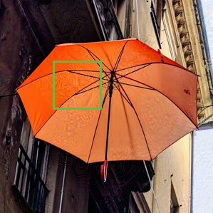
(a) modified input

(b) modified input

(c) modified input

(d) high strength

(e) medium strength

(f) low strength

(g) modified input (enlarged)

(h) modified input (enlarged)

(i) modified input (enlarged)

Figure 2: Localized attacks with different relative total strengths. The strength maps (d), (e), and (f), which are based on Perlin noise, scaled such that the relative total strength is $0.43$, $0.14$, and $0.04$, are used to create the adversarial examples in (a), (b), and (c), respectively. In each case, the attacked image is classified as slug with a certainty greater than $99\text{\,}\mathrm{\char 37\relax}$. The attacks took 14, 17, and 86 iterations. (g), (h), and (i) are enlarged versions of the marked regions in (a), (b), and (c).

The main technical observation, based on which we hide attacks, is the fact that one can weigh and apply attacks locally in a precise sense: During prediction, a convolutional neural network extracts features from an input image, condenses the information contained therein, and conflates it, in order to obtain its best guess for classification. Where exactly in an image a certain feature is located is of minor consequence compared to how strongly it is expressed [32, 33]. As a result, we find that during BIM’s update, it is not strictly necessary to apply the computed perturbation evenly across the entire image. Instead, one may choose to leave parts of the image unchanged, or perturb some pixels more or less than others, i. e. one may localize the attack. This can be directly incorporated into Equation 2 by setting an individual value for $\epsilon$ for every pixel.

For an input image $x\in\left[0,1\right]^{w\times h\times c}$ of width $w$ and height $h$ with $c$ color channels, we formalize this by setting a strength map $\mathcal{E}\in\left[0,1\right]^{w\times h}$ that holds an update magnitude for each pixel. Such a strength map can be interpreted as a grayscale image where the brightness of a pixel corresponds to how strongly the respective pixel in the input image is modified. The adaptation rule (2) of BIM is changed to the update rule

$$x_{ijk}\leftarrow x_{ijk}-\epsilon\cdot\mathcal{E}_{ijk}\cdot\mathrm{sign}[\nabla_{x}J(x,y)]$$ (3)

for all pixel values $(i,j,k)$. In order to be able to express the overall strength of an attack, for a given strength map $\mathcal{E}$ of size $w$ by $h$, we call

$$\kappa(\mathcal{E})=\frac{\sum_{i,j\in\overline{w}\times\overline{h}}\mathcal{E}_{i,j}}{w\cdot h}$$ (4)

the relative total strength of $\mathcal{E}$, where for $n\in\mathbb{N}$ we let $\overline{n}=\{1,\dots,n\}$ denote the set of natural numbers from $1$ to $n$. In the special case where $\mathcal{E}$ only contains either black or white pixels, $\kappa(\mathcal{E})$ is the ratio of white pixels, i. e. the number of attacked pixels over the total number of pixels in the attacked image.

As long as the scope of the attack, i. e. $\kappa(\mathcal{E})$, remains large enough, adversarial attacks can still be carried out successfully – if not as easily – with more iterations required until the desired certainty is reached. This leads to the attacked pixels being perturbed more, which in turn leads to even more pronounced artifacts. Given a strength map $\mathcal{E}$, it can be modified to increase or decrease $\kappa(\mathcal{E})$ by adjusting its brightness or by applying appropriate morphological operations. See Figure 2 for a demonstration that uses pseudo-random noise as a strength map.

2.2 Entropy-based attacks

The crucial component necessary for “hiding” adversarial attacks is choosing a strength map $\mathcal{E}$ that appropriately considers human perceptual biases. The strength map essentially determines which “norm” is chosen in Equation 1. If it differs from a uniform weighting, the norm considers different regions of the image differently. The choice of the norm is critical when discussing the visibility of adversarial attacks. Methods that explicitly minimize the $\ell_{p}$ norm of the perturbation for some $p$, only “accidentally” lead to perturbations that are hard to detect visually, since the $\ell_{p}$ norm does not actually resemble e. g. the human visual focus for the specific image. We propose to instead make use of how humans perceive images and to carefully choose those pixels where the resulting artifacts will not be noticeable.

Instead of trying to hide our attack in the background or “where an observer might not care to look”, we instead focus on those regions where there is high local complexity. This choice is based on the rational that humans inspect images in saccadic moves, and a focus mechanism guides how a human can process highly complex natural scenes efficiently in a limited amount of time. Visual interest serves as a selection mechanism, singling out relevant details and arriving at an optimized representation of the given stimuli [34]. We rely on the assumption that adversarial attacks remain hidden if they do not change this scheme. In particular, regions which do not attract focus in the original image should not increase their level of interest, while relevant parts can, as long as the adversarial attack is not adding additional relevant details to the original image.

Due to its dependence on semantics, it is hard – if not impossible – to agnostically compute the magnitude of interest for specific regions of an image. Hence, we rely on a simple information theoretic proxy, which can be computed based on the visual information in a given image: the entropy in a local region. This simplification relies on the observation that regions of interest such as edges typically have a higher entropy than homogeneous regions and the entropy serves as a measure for how much information is already contained in a region – that is, how much relative difference would be induced by additional changes in the region.

Algorithmically, we compute the local entropy at every pixel in the input image as follows: After discarding color, we bin the gray values, i. e. the intensities, in the neighborhood of pixel $i,j$ such that $B_{i,j}$ contains the respective occurrence ratios. The occurrence ratios can be interpreted as estimates of the intensity probability in this neighborhood, hence the local entropy $S_{i,j}$ can be calculated as the Shannon entropy

$$S_{i,j}=-\sum_{p\in B_{i,j}}p\log p.$$ (5)

Through this, we obtain a measure of local complexity for every pixel in the input image, and after adjusting the overall intensity, we use it as suggested above to scale the perturbation pixel-wise during BIM’s update. In other words, we set

$$\mathcal{E}=\phi(S)$$ (6)

where $\phi$ is a nonlinear mapping, which adjusts the brightness. The choice of a strength map based on the local entropy of an image allows us to perform an attack as straightforward as BIM, but localized, in such a way that it does not produce visible artifacts, as we will see in the following experiments.

While we could attach our technique to any attack that relies on gradients, we use BIM because of the aforementioned advantages including simplicity, versatility, and robustness, but also because as the direct successor to FGSM we consider it the most typical attack at present. As a method of performing adversarial attacks, we refer to our method as the Entropy-based Iterative Method (EbIM).

3 A study of how humans perceive adversarial examples

It is often claimed that adversarial attacks are imperceptible. While this can be the case, there are many settings in which it does not necessarily hold true – as can be seen in Figure 1. When robust networks are considered and an attack is expected to reliably and efficiently produce adversarial examples, visible artifacts appear. This motivated us to consider human visual perception directly and thereby our method. To confirm that there are in fact differences in how adversarial examples produced by BIM and EbIM are perceived, we conducted a user study with $35$ participants.

3.1 Generation of adversarial examples

To keep the course of the study manageable, so as not to bore our relatively small number of participants, and still acquire statistically meaningful (i. e. with high statistical power) and comparable results, we randomly selected only $20$ labels and $4$ samples per label from the validation set of the ILSVRC 2012 classification challenge [35], which gave us a total of $80$ images. For each of these $80$ images we generated a targeted high confidence adversarial example using BIM and another one using EbIM – resulting in a total of $240$ images. We set a fixed target class and the target certainty to $0.99$. We attacked the pretrained Inception v3 model [36] as provided by keras [37]. We set the parameters of BIM to $\epsilon=1.0$, $stepsize=0.004$ and $max\_iterations=1000$. For EbIM, we binarized the entropy mask with a threshold of $4.2$. We chose these parameters such that the algorithms can reliably generate targeted high certainty adversarial examples across all images, without requiring expensive per-sample parameter searches.

3.2 Study design

For our study, we assembled the images in pairs according to three different conditions:

1. The original image versus itself.

2. The original image versus the adversarial example generated by BIM.

3. The original image versus the adversarial example generated by EbIM.

This resulted in $240$ pairs of images that were to be evaluated during the study.

All image pairs were shown to each participant in a random order – we also randomized the positioning (left and right) of the two images in each pair. For each pair, the participant was asked to determine whether the two images were identical or different. If the participant thought that the images were identical they were to click on a button labeled “Identical” and otherwise on a button labeled “Different” – the ordering of the buttons was fixed for a given participant but randomized when they began the study. To facilitate completion of the study in a reasonable amount of time, each image pair was shown for $5$ seconds only; the participant was, however, able to wait as long as they wanted until clicking on a button, whereby they moved on to the next image pair.

3.3 Hypotheses tests

Our hypothesis was that it would be more difficult to perceive the changes in the images generated by EbIM than by BIM. We therefore expect our participants to click “Identical” more often when seeing an adversarial example generated by EbIM than when seeing an adversarial generated by BIM.

As a test statistic, we compute for each participant and for each of the three conditions separately, the percentage of time they clicked on “Identical”. The values can be interpreted as a mean if we encode “Identical” as $1$ and “Different” as $0$. Hereinafter we refer to these mean values as $\mu_{\text{BIM}}$ and $\mu_{\text{EbIM}}$. For each of the three conditions, we provide a boxplot of the test statistics in Figure 3 – the scores of EbIM are much higher than BIM, which indicates that it is in fact much harder to perceive the modifications introduced by EbIM compared to BIM. Furthermore, users almost always clicked on “Identical” when seeing two identical images.

Figure 3: Percentage of times users clicked on “Identical” when seeing two identical images (condition (i), blue box), a BIM adversarial (condition (ii), orange box), or an EbIM adversarial (condition (iii), green box).

Finally, we can phrase our belief as a hypothesis test. We determine whether we can reject the following five hypotheses:

1. $H_{0}\colon\mu_{\text{BIM}}\geq\mu_{\text{EbIM}}$, i. e. attacks using BIM are as hard or harder to perceive than EbIM.

2. $H_{0}\colon\mu_{\text{BIM}}\geq 0.5$, i. e. whether attacks using BIM are easier or harder to perceive than a random prediction

3. $H_{0}\colon\mu_{\text{EbIM}}\leq 0.5$, i. e. whether attacks using EbIM are easier or harder to perceive than a random prediction

4. $H_{0}\colon\mu_{\text{BIM}}\geq\mu_{\text{NONE}}$, i. e. whether attacks using BIM are as easy or easier to perceive than identical images.

5. $H_{0}\colon\mu_{\text{EbIM}}\geq\mu_{\text{NONE}}$, i. e. whether attacks using EbIM are as easy or easier to perceive than identical images.

We use a one-tailed t-test and the (non-parametric) Wilcoxon signed rank test with a significance level $\alpha=0.05$ in both tests. The cases (1),(4) and (5) are tested as a paired test and the other two cases (2) and (3) as one sample tests.

Because the t-test assumes that the mean difference is normally distributed, we test for normality by using the Shapiro-Wilk normality test. The Shapiro-Wilk normality test computes a p-value of $0.425$, therefore we assume that the mean difference follows a normal distribution. The resulting p-values are listed in 1 – we can reject all null hypotheses with very low p-values.

Table 1: p-values of each hypothesis (columns) under each test (rows). We reject all null hypotheses.

Test	Hyp. (1)	Hyp. (2)	Hyp. (3)	Hyp. (4)	Hyp. (5)
t-test	$2.2\text{\times}{10}^{-16}$	$1.025\text{\times}{10}^{-10}$	$2.129\text{\times}{10}^{-05}$	$2.2\text{\times}{10}^{-16}$	$2.2\text{\times}{10}^{-16}$
Wilcoxon	$1.281\text{\times}{10}^{-07}$	$9.101\text{\times}{10}^{-07}$	$6.748\text{\times}{10}^{-05}$	$1.283\text{\times}{10}^{-07}$	$1.282\text{\times}{10}^{-07}$

In order to compute the power of the t-test, we compute the effect size by computing Cohen’s d. We find that $d\approx 2.29$ which is considered a huge effect size [38]. The power of the one-tailed t-test is then approximately $1$.

We have empirically shown that adversarial examples produced by EbIM are significantly harder to perceive than adversarial examples generated by BIM. Furthermore, adversarial examples produced by EbIM are not perceived as differing from their respective originals.

4 Discussion

Adversarial attacks will remain a potential security risk on the one hand and an intriguing phenomenon that leads to insight into neural networks on the other. Their nature is difficult to pinpoint and it is hard to predict whether they constitute a problem that will be solved. To further the understanding of adversarial attacks and robustness against them, we have demonstrated two key points:

• Adversarial attacks against convolutional neural networks can be carried out successfully even when they are localized.

• By reasoning about human visual perception and carefully choosing areas of high complexity for an attack, we can ensure that the adversarial perturbation is barely perceptible, even to an astute observer who has learned to recognize typical patterns found in adversarial examples.

This has allowed us to develop the Entropy-based Iterative Method (EbIM), which performs adversarial attacks against convolutional neural networks that are hard to detect visually even when their magnitude is considerable with regards to an $\ell_{p}$-norm. It remains to be seen how current adversarial defenses perform when confronted with entropy-based attacks, and whether robust networks learn special kinds of features when trained adversarially using EbIM.

Through our user study we have made clear that not all adversarial attacks are imperceptible. We hope that this is only the start of considering human perception explicitly during the investigation of deep neural networks in general and adversarial attacks against them specifically. Ideally, this would lead to a concise definition of what constitutes an adversarial example.

Appendix

For illustrative purposes, we include a number of adversarial examples that result from attacks using the Basic Iterative Method (BIM) and our Entropy-based Iterative Method (EbIM), against Inception v3 and AlexNet, in LABEL:fig:inception-fgsm,fig:inception-entropy,fig:alexnet-fgsm,fig:alexnet-entropy. The images are best viewed digitally on a screen, with the ability to zoom in. It should become clear how BIM leads to perceivable artifacts in low-entropy regions, which is avoided when EbIM is employed. At the same time, certain (comparably hard to see) artifacts result from EbIM, too, particularly around pronounced edges. Note that this effect might be mitigated by smarter choices with regards to the morphological operations applied to the pixel-wise entropy before it is used as a strength map.

(a)

(b)

(c)

(d)

(e)

(f)

(g)

(h)

(i)

(j)

(k)

(l)

Figure 4: Twelve adversarial example resulting from attacks against Inception v3 using the Basic Iterative Method.

(a)

(b)

(c)

(d)

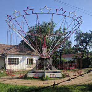
(e)

(f)

(g)

(h)

(i)

(j)

(k)

(l)

Figure 5: Twelve adversarial example resulting from attacks against Inception v3 using our Entropy-based Iterative Method.

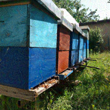
(a)

(b)

(c)

(d)

(e)

(f)

(g)

(h)

(i)

(j)

(k)

(l)

Figure 6: Twelve adversarial example resulting from attacks against AlexNet using the Basic Iterative Method.

(a)

(b)

(c)

(d)

(e)

(f)

(g)

(h)

(i)

(j)

(k)

(l)

Figure 7: Twelve adversarial example resulting from attacks against AlexNet using our Entropy-based Iterative Method.

References

- [1] Alex Krizhevsky, Ilya Sutskever and Geoffrey E. Hinton “ImageNet Classification with Deep Convolutional Neural Networks” In Advances in Neural Information Processing Systems 25, 2012 DOI: 10.1145/3065386
- [2] Christian Szegedy, Wojciech Zaremba, Ilya Sutskever, Joan Bruna, Dumitru Erhan, Ian J. Goodfellow and Rob Fergus “Intriguing properties of neural networks”, 2013
- [3] Jiawei Su, Danilo Vasconcellos Vargas and Kouichi Sakurai “One pixel attack for fooling deep neural networks”, 2017
- [4] Alexey Kurakin, Ian J. Goodfellow and Samy Bengio “Adversarial examples in the physical world”, 2016
- [5] Nicolas Papernot, Patrick D. McDaniel, Ian J. Goodfellow, Somesh Jha, Z. Celik and Ananthram Swami “Practical Black-Box Attacks against Deep Learning Systems using Adversarial Examples”, 2016
- [6] Anirban Chakraborty, Manaar Alam, Vishal Dey, Anupam Chattopadhyay and Debdeep Mukhopadhyay “Adversarial Attacks and Defences: A Survey”, 2018
- [7] Ian J. Goodfellow, Jonathon Shlens and Christian Szegedy “Explaining and Harnessing Adversarial Examples”, 2014
- [8] Yan Luo, Xavier Boix, Gemma Roig, Tomaso Poggio and Qi Zhao “Foveation-based Mechanisms Alleviate Adversarial Examples”, 2015
- [9] Moustapha Cisse, Piotr Bojanowski, Edouard Grave, Yann Dauphin and Nicolas Usunier “Parseval Networks: Improving Robustness to Adversarial Examples” In ICML, 2017
- [10] Andrew Ilyas, Shibani Santurkar, Dimitris Tsipras, Logan Engstrom, Brandon Tran and Aleksander Madry “Adversarial Examples Are Not Bugs, They Are Features”, 2019
- [11] Nicolas Papernot, Patrick McDaniel, Xi Wu, Somesh Jha and Ananthram Swami “Distillation as a Defense to Adversarial Perturbations Against Deep Neural Networks” In 2016 IEEE Symposium on Security and Privacy (SP) IEEE, 2016 DOI: 10.1109/sp.2016.41
- [12] Aleksander Madry, Aleksandar Makelov, Ludwig Schmidt, Dimitris Tsipras and Adrian Vladu “Towards Deep Learning Models Resistant to Adversarial Attacks” In Proceedings of the International Conference on Learning Representations (ICLR), 2018
- [13] Francesco Crecchi, Davide Bacciu and Battista Biggio “Detecting Adversarial Examples through Nonlinear Dimensionality Reduction” In Proceedings of the European Symposium on Artificial Neural Networks, Computational Intelligence and Machine Learning (ESANN), 2019
- [14] Reuben Feinman, Ryan R. Curtin, Saurabh Shintre and Andrew B. Gardner “Detecting Adversarial Samples from Artifacts”, 2017
- [15] Kathrin Grosse, Praveen Manoharan, Nicolas Papernot, Michael Backes and Patrick McDaniel “On the (Statistical) Detection of Adversarial Examples”, 2017
- [16] Jan Hendrik Metzen, Tim Genewein, Volker Fischer and Bastian Bischoff “On Detecting Adversarial Perturbations”, 2017
- [17] Nicholas Carlini and David A. Wagner “Towards Evaluating the Robustness of Neural Networks” In 2017 IEEE Symposium on Security and Privacy (SP), 2017
- [18] Anish Athalye, Nicholas Carlini and David Wagner “Obfuscated Gradients Give a False Sense of Security: Circumventing Defenses to Adversarial Examples” In ICML, 2018
- [19] Dimitris Tsipras, Shibani Santurkar, Logan Engstrom, Alexander Turner and Aleksander Madry “Robustness May Be at Odds with Accuracy” In Proceedings of the International Conference on Learning Representations (ICLR), 2019
- [20] Preetum Nakkiran “Adversarial Robustness May Be at Odds With Simplicity”, 2019
- [21] Daniel L.. Yamins and James J. DiCarlo “Using goal-driven deep learning models to understand sensory cortex” In Nature Neuroscience 19, 2016, pp. 356–365 DOI: 10.1038/nn.4244
- [22] Rishi Rajalingham, Elias B. Issa, Pouya Bashivan, Kohitij Kar, Kailyn Schmidt and James J. DiCarlo “Large-Scale, High-Resolution Comparison of the Core Visual Object Recognition Behavior of Humans, Monkeys, and State-of-the-Art Deep Artificial Neural Networks” In Journal of Neuroscience 38.33 Society for Neuroscience, 2018, pp. 7255–7269 DOI: 10.1523/JNEUROSCI.0388-18.2018
- [23] Gamaleldin Elsayed, Shreya Shankar, Brian Cheung, Nicolas Papernot, Alexey Kurakin, Ian Goodfellow and Jascha Sohl-Dickstein “Adversarial Examples that Fool both Computer Vision and Time-Limited Humans” In Advances in Neural Information Processing Systems 31, 2018, pp. 3910–3920
- [24] Heiko Wersing, Jochen J. Steil and Helge Ritter “A Competitive-Layer Model for Feature Binding and Sensory Segmentation” In Neural Computation 13.2, 2001, pp. 357–387 DOI: 10.1162/089976601300014574
- [25] Michael Ibbotson and Bart Krekelberg “Visual perception and saccadic eye movements” Sensory and motor systems In Current Opinion in Neurobiology 21.4, 2011, pp. 553–558 DOI: 10.1016/j.conb.2011.05.012
- [26] Michael Lewicki, Bruno Olshausen, Annemarie Surlykke and Cynthia Moss “Scene analysis in the natural environment” In Frontiers in Psychology 5, 2014, pp. 199 DOI: 10.3389/fpsyg.2014.00199
- [27] Frank Jäkel, Manish Singh, Felix A. Wichmann and Michael H. Herzog “An overview of quantitative approaches in Gestalt perception” Quantitative Approaches in Gestalt Perception In Vision Research 126, 2016, pp. 3–8 DOI: 10.1016/j.visres.2016.06.004
- [28] Alexey Kurakin, Ian J. Goodfellow and Samy Bengio “Adversarial Machine Learning at Scale”, 2016
- [29] Seyed-Mohsen Moosavi-Dezfooli, Alhussein Fawzi and Pascal Frossard “DeepFool: A Simple and Accurate Method to Fool Deep Neural Networks” In 2016 IEEE Conference on Computer Vision and Pattern Recognition (CVPR), 2016, pp. 2574–2582
- [30] Jonas Rauber, Wieland Brendel and Matthias Bethge “Foolbox v0.8.0: A Python toolbox to benchmark the robustness of machine learning models”, 2017
- [31] Lea Schönherr, Katharina Kohls, Steffen Zeiler, Thorsten Holz and Dorothea Kolossa “Adversarial Attacks Against Automatic Speech Recognition Systems via Psychoacoustic Hiding”, 2018
- [32] Sara Sabour, Nicholas Frosst and Geoffrey E. Hinton “Dynamic Routing Between Capsules” In Advances in Neural Information Processing Systems, 2017
- [33] Tom B. Brown, Dandelion Mané, Aurko Roy, Martín Abadi and Justin Gilmer “Adversarial Patch”, 2017
- [34] Marisa Carrasco “Visual attention: The past 25 years” In Vision Research 51, 2011, pp. 1484–1525
- [35] Olga Russakovsky et al. “ImageNet Large Scale Visual Recognition Challenge” In International Journal of Computer Vision (IJCV) 115.3, 2015, pp. 211–252 DOI: 10.1007/s11263-015-0816-y
- [36] Christian Szegedy, Vincent Vanhoucke, Sergey Ioffe, Jonathon Shlens and Zbigniew Wojna “Rethinking the Inception Architecture for Computer Vision” In 2016 IEEE Conference on Computer Vision and Pattern Recognition (CVPR), 2016, pp. 2818–2826
- [37] François Chollet “Keras”, 2015 URL: https://keras.io
- [38] Shlomo S. Sawilowsky “New Effect Size Rules of Thumb” In Journal of Modern Applied Statistical Methods 8.2 Wayne State University Library System, 2009, pp. 597–599 DOI: 10.22237/jmasm/1257035100