Propagation of ultra-short, resonant, ionizing laser pulses in rubidium vapor

Abstract

We investigate the propagation of ultra-short laser pulses in atomic rubidium vapor. The pulses are intensive enough to ionize the atoms and are directly resonant with the 780 nm $D_{2}$ line. We derive a relatively simple theory for computing the nonlinear optical response of atoms and investigate the competing effects of strong resonant nonlinearity and ionization in the medium using computer simulations. A nonlinear self-channeling of pulse energy is found to produce a continuous plasma channel with complete ionization. We evaluate the length, width and homogeneity of the resulting plasma channel for various values of pulse energy and initial focusing to identify regimes optimal for applications in plasma-wave accelerator devices such as that being built by the AWAKE collaboration at CERN. Similarities and differences with laser pulse filamentation in atmospheric gases are discussed.

I Introduction

The propagation of femtosecond laser pulses in various optical media is an active field of study with many applications. In particular, pulses powerful enough to ionize atoms and molecules of gases they propagate through have been studied intensely in the past 2-3 decades. Their propagation is governed by the dynamical competition between optical nonlinearities of various orders, intensity clamping due to multiphoton ionization and refractive index changes due to plasma generation. The competition between self-focusing and de-focusing effects lead to the formation of filaments, i.e. long, extended domains along the pulse propagation direction with strong localization in the transverse plane where gas is ionized. The precise mechanisms through which these plasma channels are created and light filaments maintained have been investigated extensively both theoretically and experimentally Bergé (1998); Couairon and Mysyrowicz (2007); Bergé et al. (2007); Kandidov et al. (2009); Kolesik and Moloney (2013).

A very similar problem arose recently in the context of the Advanced Proton Driven Plasma Wakefield Acceleration Experiment (AWAKE) experiment at CERN. AWAKE is a proton-driven plasma wakefield acceleration experiment, the first of its kind, which uses high-energy proton bunches to drive wakefields in a plasma for electron acceleration Caldwell et al. (2016); Gschwendtner et al. (2016); Adli et al. (2018). Central to the device is a 10 m long rubidium vapor cell where the proton bunch interacts with the plasma serving as an energy exchange medium between the protons and the injected electrons. Under appropriate conditions, the self-modulation instability breaks up the proton bunch which then resonantly drives the plasma wakefields. Important factors for success are high plasma homogeneity as well as a quasi-instantaneous plasma creation for seeding the instability during the time the proton bunch is in the cell. This is achieved by ionizing the rubidium vapor in the temperature controlled cell by a powerful fs laser pulse propagating simultaneously with the proton bunch. The problem is at first sight almost identical to filamentation studies in atmospheric gases as the formation of a long plasma channel is required by a powerful, ultra-short laser pulse.

But there are also some fundamental differences. First of all, the 780 nm AWAKE laser is directly resonant with the $D_{2}$ line of rubidium, the transition between the $5\mathrm{S}_{1/2}$ ground state to the $5\mathrm{P}_{3/2}$ excited state and very close to resonance with the 776 nm $5\mathrm{P}_{3/2}\rightarrow 5\mathrm{D}_{5/2},5\mathrm{D}_{3/2}$ transitions. This means that there is very strong nonlinear optical interaction between the pulse and the vapor at arbitrarily low intensities. Because this nonlinearity is much stronger than the ones given by the usual nonresonant nonlinear optical coefficients, we get a sizeable response from the medium even though the initial vapor density is $10^{14}-10^{15}\mathrm{~{}1/cm^{3}}$, orders of magnitude less dense than atmospheric gases. The effect of such a single-photon resonance is completely missing from usual filamentation studies, though the effects of resonant two- and three-photon transitions on the process have been investigated recently Doussot et al. (2016, 2017). Second, high plasma homogeneity is required which must be achieved through 100 % ionization of the initially homogeneous vapor - this means that plasma density gradients will absent everywhere but the boundary of the plasma channel. Third, contrary to usual cases of laser filamentation where the medium is effectively transparent until the intensity is high enough to ionize the gas, here we have a resonantly absorbing medium until all the atoms have been completely ionized. At this point however, the medium is rendered almost transparent. All this means that we have a hybrid system - around the pulse edge, where intensity is small, we may expect phenomena familiar from resonant nonlinear optics Boshier and Sandle (1982); LAMB (1971); de Lamare et al. (1994); Delagnes and Bouchene (2008). On the other hand, around the pulse center where intensity is large we may expect processes similar to the ones encountered in filamentation studies Fill (1994); Couairon and Mysyrowicz (2007); Bergé et al. (2007); Kolesik and Moloney (2013).

In order to investigate the propagation of ultra-short, ionizing laser pulses resonant with a transition from the atomic ground state in rubidium vapor, we develop a relatively simple model for the nonlinear optical response of the atoms and perform computer simulations to investigate propagation phenomena. We analyze the competing dynamics of self-focusing, nonlinear absorption and diffraction that govern the reshaping of the pulse in the medium and the geometry of the plasma channel left behind after the interaction. Our aim is to identify the requirements for the formation of a clean, continuous plasma channel with constant plasma density whose transverse dimensions are sufficient for use in plasma wake-field acceleration devices.

II Theory

II.1 Basic approach

We set out to calculate the long range ($\sim$ 10 m) propagation of 780 nm wavelength, $\sim$ 100 fs laser pulses in Rb vapor. The pulses are intense enough to ionize via multiphoton or tunnel ionization directly from the ground state ($I\sim\mathrm{~{}TW/cm^{2}})$, but are also resonant with the transition from the atomic ground state to the first excited state. The vapor density is $\sim 10^{14}-10^{15}\mathrm{~{}1/cm}^{3}$, far below the atmospheric densities usually considered in filamentation studies. In order to calculate pulse propagation, we need a wave equation for the light-field and couple it with the atomic response functions. The transient atomic response is expected to be dominated by the single photon resonances, so the traditional approach of using nonlinear susceptibility functions with various powers of the intensity does not work. The classical formulas for anomalous dispersion in the vicinity of an absorption line are also useless at these timescales, we expect that Rabi-like oscillations will yield the atomic response, augmented by ionization losses. Ab-initio methods that calculate the evolution of the electron wavefunction in space from a bound state to continuum states are theoretically sound and can treat this situation naturally, but are computationally too costly for using to calculate long range propagation and parameter scans. To make extended calculations feasible, we consider an axially symmetric system, physical quantities are assumed to depend only on the $r$ coordinate in the transverse plane.

II.2 Model equations

We assume that the laser field is linearly polarized and employ an envelope description of both the electric field $E$ and material response $P$ of the rubidium vapor, separating the central frequency of the laser: $E(\vec{r},z,t)=\frac{1}{2}\mathcal{E}(\vec{r},z,t)\exp(ik_{0}z-\omega_{0}t)+c.c.$ and $P(\vec{r},z,t)=\frac{1}{2}\mathcal{P}(\vec{r},z,t)\exp(ik_{0}z-\omega_{0}t)+c.c.$ . Here $z$ is the propagation direction, $\vec{r}$ is the position in the plane transverse to it and $\omega_{0}=k_{0}c$ the central frequency of the laser. The medium response is entirely contained in the polarization function $P(\vec{r},z,t)$, linear and nonlinear parts are not separated explicitly. Using the standard transformation to a moving reference frame $\xi=z$, $\tau=t-z/c$, employing the paraxial approximation for propagation along $z$, rewriting the wave equation for the envelopes in frequency space $\tilde{\mathcal{E}}(\vec{r},\xi,\omega)=\mathfrak{F}\{\mathcal{E}(\vec{r},\xi,\tau)\}$, $\tilde{\mathcal{P}}(\vec{r},\xi,\omega)=\mathfrak{F}\{\mathcal{P}(\vec{r},\xi,\tau)\}$ (where $\mathfrak{F}\{\ldotp\}$ denotes the time-Fourier transform) and finally employing the Slowly Evolving Wave Approximation (SEWA) Brabec and Krausz (1997); Couairon et al. (2011) we arrive at the wave equation:

$$\nabla_{\perp}^{2}\tilde{\mathcal{E}}(\vec{r},\xi,\omega) +i2(k_{0}+k)\partial_{\xi}\tilde{\mathcal{E}}(\vec{r},\xi,\omega)=$$ (1)

$$-(k_{0}+k)^{2}\tilde{\mathcal{P}}(\vec{r},\xi,\omega)/\epsilon_{0}.$$

Here $k,\omega$ are the wavevector and the angular frequency of the various components offset from $k_{0}$ and $\omega_{0}$, $k=\omega/c$ and $\epsilon_{0}$ is the vacuum permittivity. The SEWA approximation that we use for deriving a first order wave equation has been developed for treating the propagation of ultra-short (few-cycle) pulses and is much less restrictive than the Slowly Varying Envelope Approximation (SVEA) widely used in resonant nonlinear optics. In particular, it is still valid if the pulse develops a sharp leading edge during propagation.

Atomic rubidium has a single valence electron outside a closed shell and an atomic transition from the $\mathrm{5S_{1/2}}$ ground state to the $\mathrm{5P_{3/2}}$ first excited state at $780\mathrm{~{}nm}$ (the $D_{2}$ line), precisely the same as the central wavelength of the Ti:sapphire laser used at the AWAKE experiment Gschwendtner et al. (2016). Furthermore, there are two transitions from the first excited state to higher atomic states still well within the bandwidth of the laser: the $\mathrm{5P_{3/2}\rightarrow 5D_{3/2}}$ transition at 775.9 nm and the $\mathrm{5P_{3/2}\rightarrow 5D_{5/2}}$ one at 775.8 nm Steck (2009); Kramida et al. (2018), see Fig. 1. The transition from the ground state to $\mathrm{5P_{1/2}}$ at 794.8 nm is well out of resonance for this setup, so there are three excited states resonantly accessible from the ground state because of the coupling to the laser light. A “minimal” model of the atom used to calculate the optical response that is lightweight enough to be employed in extended propagation calculations must therefore include these four states as well as the process of photoionization from theses states.

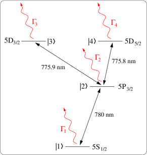
Figure 1: Electronic levels of the Rb atom that are included in the model and their numbering. Three excited states are resonantly accessible from the ground state, ionization leads to level loss from each of the levels.

We start by separating the material response into parts describing atomic polarization due to resonant transitions between bound states and an absorption term due to ionization processes: $\mathcal{P}=\mathcal{P}_{atomic}+\mathcal{P}_{ionization}$. We write the Schrödinger equation for the probability amplitudes of the four quantum states in the spirit of resonant nonlinear optics. We take the quantization axis of the atomic angular momentum parallel to the direction of polarization, so the magnetic quantum number $m$ is conserved. Assuming the initial state of the atom to be in the ground state, without any constraint on generality we may use the set of atomic quantum states $\{|1\rangle=|5S_{1/2},m=1/2\rangle,|2\rangle=|5P_{3/2},m=1/2\rangle,|3\rangle=|5D_{3/2},m=1/2\rangle,|4\rangle=|5S_{5/2},m=1/2\rangle\}$ as an expansion basis for the atomic wave function with time dependent expansion coefficients $\alpha_{j}(t)$ (the other linkage pattern with $m=-1/2$ is symmetrical to this one). Note that this separation is possible because radiative transitions that could yield transitions between states of different $m$ are completely negligible on the $\sim$100 fs timescale. The wave function is thus written as:

$$|\psi(t)\rangle=\sum_{j=1}^{4}\alpha_{j}(t)|j\rangle.$$ (2)

Next we introduce the transformed probability amplitudes $a_{j}(t)$ by applying the phase transformation with respect to $\omega_{0}$ and $\omega_{2}$ as:

$$a_{1}(t) =\alpha_{1}(t)e^{i(\omega_{2}-\omega_{0})t}$$ (3)

$$a_{2}(t) =\alpha_{2}(t)e^{i\omega_{2}t}$$

$$a_{3}(t) =\alpha_{3}(t)e^{i(\omega_{2}+\omega_{0})t}$$

$$a_{4}(t) =\alpha_{4}(t)e^{i(\omega_{2}+\omega_{0})t}$$

Here $\omega_{2}$ is the energy of the first excited state $|2\rangle$ divided by $\hbar$ and the transformation amounts choosing this energy as reference and to transforming to a reference fame rotating with the optical field. Using the Hamiltonian

$$\hat{H}=\sum_{j=1}^{4}\hbar\omega_{j}|j\rangle\langle j|-\hat{d}E$$ (4)

we obtain the equations for the probability amplitudes in the moving frame:

$$\partial_{\tau}a_{1}= -i\Delta_{21}a_{1}+\frac{i}{2}\Omega^{*}D_{21}a_{2}-\frac{\Gamma_{1}}{2}a_{1}$$ (5)

$$\partial_{\tau}a_{2}= \frac{i}{2}\bigl{(}\Omega D_{21}a_{1}+\Omega^{*}D_{32}a_{3}+\Omega^{*}D_{42}a_{4}\bigr{)}-\frac{\Gamma_{2}}{2}a_{2}$$

$$\partial_{\tau}a_{3}= i\Delta_{32}a_{3}+\frac{i}{2}\Omega D_{32}a_{2}-\frac{\Gamma_{3}}{2}a_{3}$$

$$\partial_{\tau}a_{4}= i\Delta_{42}a_{4}+\frac{i}{2}\Omega D_{42}a_{2}-\frac{\Gamma_{4}}{2}a_{4}$$

Here we have introduced the notation $\Delta_{kl}=\omega_{0}-(\omega_{k}-\omega_{l})$ for the detuning of the central laser frequency from the relevant atomic transitions and used the Rotating Wave approximation (RWA). We have also introduced the Rabi frequency for a unit dipole $\Omega(\tau)=\mathcal{E}(\tau)ea_{0}/\hbar$ ($e$ is the elementary charge and $a_{0}$ the Bohr radius) and written the dipole matrix elements in units of $ea_{0}$ as well, $\langle k|\hat{d}|l\rangle=D_{kl}ea_{0}$. $\Gamma_{k}$ are phenomenological loss terms for the level probabilities that describe photoionization and we have suppressed the explicit space and time dependence of $a_{k}$, $\Gamma_{k}$ and $\Omega$ for brevity. The material parameters $\omega_{k}$ and $D_{kl}$ are obtained from the literature Kramida et al. (2018); Steck (2009); Safronova et al. (2004), their numerical values are quoted in the appendix. The intensity dependent photoionization rates $\Gamma_{k}$ for the two lower atomic levels $|1\rangle$ and $|2\rangle$are obtained from the so-called PPT formulas Perelomov et al. (1966, 1967); Perelomov and Popov (1967) that describe both multiphoton ionization and tunnel ionization in a unified way. For the two higher lying states $|3\rangle,|4\rangle$ an experimentally measured photoionization cross section is used as detailed in the appendix. Solving Eqs. 5 at any point in space allows us to calculate the atomic part of the polarization $P_{atomic}=\langle\psi|\hat{d}|\psi\rangle$ for insertion into the wave equation.

The wave equation in frequency space Eq. 1 is written in terms of $\tilde{\Omega}(\vec{r},\xi,\omega)$:

$$\partial_{\xi}\tilde{\Omega}=\frac{i}{2}\frac{c}{\omega_{0}+\omega}\nabla_{\perp}^{2}\tilde{\Omega}+i\kappa_{1}\frac{\omega_{0}+\omega}{c}\tilde{p}-\kappa_{2}\tilde{\mathcal{Q}}.$$ (6)

Here the first term describes diffraction, the second term is due to atomic polarization due to transitions between bound states:

$$\tilde{p}=\mathfrak{F}\{p(\vec{r},\xi,\tau)\}=\mathfrak{F}\{D_{21}a_{1}^{*}a_{2}+D_{23}a_{2}^{*}a_{3}+D_{24}a_{2}^{*}a_{4}\}.$$ (7)

The third term corresponds to $P_{ionization}$ and is purely an energy loss term derived from the requirement that the laser pulse should loose an appropriate number times the energy of a photon each time an atom is ionized:

$$\tilde{\mathcal{Q}}=\mathfrak{F}\{\mathcal{Q}(\vec{r},\xi,\tau)\}=\mathfrak{F}\left\{\sum_{j}n_{j}\frac{\Gamma_{j}|a_{j}|^{2}}{\Omega^{*}}\right\}$$ (8)

The numbers $n_{j}$ are the photon numbers associated with the ionization process from each of the atomic states. Note that they can be intensity dependent non-integers as the ionization rates may contain contributions from higher photon-number processes (see Eqs. 14), though they are practically always close to the minimal number of required photons in our case. The constants appearing in Eq. 6 are given by:

$$\kappa_{1}=\frac{\mathcal{N}e^{2}a_{0}^{2}}{\hbar\epsilon_{0}} \kappa_{2}=\frac{\eta_{0}\omega_{0}\mathcal{N}e^{2}a_{0}^{2}}{\hbar}$$ , (9)

where $\mathcal{N}$ is the vapor density and $\eta_{0}$ is the impedance of vacuum. Equations 5 and 6 together with the relations 7 and 8 constitute the set of equations we have to solve for the investigation of our problem.

III Propagation calculations

The equations were solved numerically assuming an axially symmetric system, i.e. all quantities were taken to depend on the propagation direction $z$ and the transverse radial coordinate $r$. The incident pulse was assumed to be a Gaussian beam with the waist located at $z=0$ the start of the interaction, the initial beam diameter $d$ (intensity FWHM width) and pulse energy $E_{0}$ being the two parameters varied during the parameter scans. The temporal shape of the incident pulse envelope was a hyperbolic secant $\mathrm{sech}(t/\tau_{p})$ with $\tau_{p}=85.0944\mathrm{~{}fs}$ which translates to a pulse duration of 150 fs. $\mathcal{N}=2\times 10^{14}/\mathrm{cm}^{3}$ vapor density was used in all calculations. Eqs. 5 were solved with a fourth-order Dormand-Prince algorithm at each step of the numerical integration of Eq. 6. A split-step operator scheme was used for the latter equation.

III.1 Pulse self-focusing and self-channeling

Pulse interaction with the rubidium vapor was first investigated for low energy pulses. With a beam waist diameter $d=1.5\mathrm{~{}mm}$ and pulse energies of $E_{0}=10^{-3}-10^{-2}\mathrm{~{}mJ}$, the initial on-axis peak intensity is $I\approx 10^{9}\mathrm{~{}W/cm^{2}}$, too small to ionize the atoms during the pulse. The spatial evolution of the on-axis radiant fluence $\mathcal{F}_{0}(z)=\int I(r=0,z,t)dt$ with propagation distance $z$ has been plotted for several values of $E_{0}$ in Fig. 2. Traces of self focusing are visible even for $E_{0}=0.003\mathrm{~{}mJ}$ as a marked deviation from an exponentially decreasing absorption curve (panel (a), blue curve) –absorption clearly still dominates though. However, for $E_{0}=0.006\mathrm{~{}mJ}$, we already have a pulse focused around $z\approx 0.15\mathrm{~{}m}$ with the peak on-axis fluence over an order of magnitude greater than its initial ($z=0$) value, despite absorption (panel (b), blue curve). The overall behavior is very similar to that found for laser propagation in a medium of resonant two-level atoms Boshier and Sandle (1982), where the nonlinear refractive index and saturable absorption were both found to contribute to self-focusing. (Note however, that those results were derived for CW beams and ionization completely absent.)

The onset of self-focusing here is considerably different from that caused by the classical intensity-dependent refractive index $n_{2}\cdot I$ in transparent media Kelley (1965); Marburger (1975). First, the required pulse power is orders of magnitude smaller as the 0.006 mJ pulse plotted in panel (b) of Fig. 2 corresponds to $P=40\mathrm{~{}MW}$. Compared with the GW power required in atmospheric density gases Couairon and Mysyrowicz (2007) and noting that vapor density in our case is five orders of magnitude smaller, it is clear that the nonlinearity in this system is about $10^{7}$ times larger. Second, the location of the nonlinear focus increases with increasing pulse energy (or power) which is different from the scalings $(P/P_{cr})^{-1/2}$ and $(P/P_{cr})^{-1}$ observed for nonresonant pulses in various power domains Fibich et al. (2005). Third, not only the overall pulse power, but also peak intensity and radiant fluence (and hence beam waist diameter) are important parameters in this system as the nonlinearity competes with both diffraction and absorption and it is easily saturated as atoms are lost from interaction via ionization. Indeed, for the $E_{0}=0.01\mathrm{~{}mJ}$ green curve in panel b) of Fig. 2, ionization probability is already close to 80% at the center of the nonlinear focus.

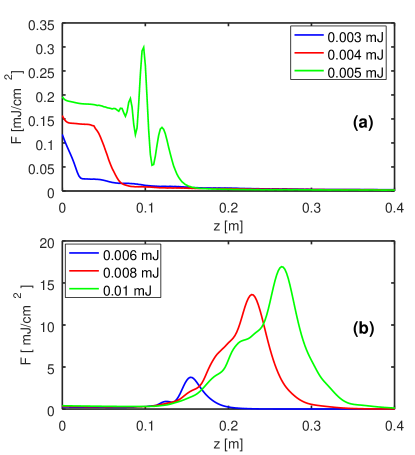
Figure 2: On-axis radiant fluence $\mathcal{F}_{0}(z)$ in $\mathrm{mJ/cm^{2}}$ as a function of propagation distance $z$ for six values of the initial pulse energy $E_{0}$.

Calculations for higher pulse energies yield interesting solutions that at first sight bear considerable resemblance to filamentation phenomena in air when self-focusing leads to plasma generation. A typical scenario is shown in Fig. 3. The spatial evolution of the radiant fluence is shown in panel (a), its on-axis value vs. propagation distance on panel (b). The plots clearly show that as the pulse propagates in the medium, the energy is focused periodically around the axis. The peaks decrease in amplitude and radial extension as the pulse progresses and energy is lost. The vapor is ionized completely close to the axis, the boundary of the plasma channel expanding and contracting repeatedly with the radial extension of the laser pulse. (Panel c) displays the spatial distribution of the final ionization probability. Note that in this case the pulse is already intense enough to ionize the atoms at $z=0$, without self-focusing.) As the pulse energy is depleted, the plasma channel narrows and eventually ends as the pulse is no longer able to ionize the atoms. Clearly, there is a dynamic competition between nonlinear polarization, absorption and diffraction that yields an irregular, quasi-periodic plasma channel.

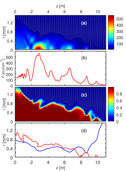
Figure 3: The propagation of a laser pulse with $E_{0}=3.5\mathrm{~{}mJ}$ in Rb vapor. The horizontal axes of all four panels is $z$, the propagation distance, with identical scaling. (a) Contour plot of $\mathcal{F}(r,z)$ $[\mathrm{mJ/cm^{2}}]$. (b) On-axis fluence $\mathcal{F}_{0}(z)$. (c) Contour plot of the final ionization probability. (d) Blue line: half-energy radius $R_{1/2}(z)$ of the beam, red line: the boundary of 98% ionization probability.

A closer look reveals some fundamental differences to laser filamentation in air and other gases. In those scenarios the gas is essentially transparent, there is little or no loss when pulse intensity is not high enough to ionize the atoms or molecules. Self-focusing increases intensity until it is stopped (or rather dynamically balanced) by a combination of diffraction, plasma defocusing, strong energy losses due to multiphoton ionization, a saturation of $n_{2}$ or the emergence of higher order defocusing nonlinearities Feit and Fleck (1974); Couairon (2003); Béjot et al. (2011); Couairon and Mysyrowicz (2007). Because a large portion of the pulse energy can propagate outside the highly intense domain, the filament may regenerate even if its central, most intense portion is blocked Courvoisier et al. (2003); Kolesik and Moloney (2004); Skupin et al. (2004). Conversely, in our case there is absorption for arbitrarily small intensities, but the absorber is easily saturable, the medium becomes transparent when it is fully ionized. Panel (d) of Fig.2 displays two curves, the boundary of 98% ionization (red line) which is a measure of the extent of the plasma channel and the ’half-energy width’ $R_{1/2}(z)$ of the laser beam (blue line). This latter is defined such that

$$\int_{0}^{R_{1/2}}2\pi r\mathcal{F}(r,z)dr=\frac{E(z)}{2}$$ (10)

i.e. exactly half of the overall energy of the pulse at any given propagation distance $z$ is contained within the domain $r\leq R_{1/2}(z)$. (A beam width parameter like the FWHM in intensity or fluence would not be very representative as the beam cross-section does not remain a Gaussian and at certain positions it does not peak at $r=0$ but may have a hollow beam structure.) The figure shows that most of the pulse energy propagates within the plasma channel where absorption and nonlinear refraction are saturated. There is a self-channeling of the energy, self-focusing by the nonlinear medium is halted by the completion of the channel with full ionization where the laser field travels through a homogeneous, transparent plasma medium. There is no further absorption because the ionization potential of the second electron of rubidium is so much higher than that of the first one. Plasma defocusing within the channel is also absent as there is no gradient of plasma density within the channel core. Diffraction is the only mechanism that makes the beam expand repeatedly. Naturally, energy is constantly lost from the front part of the pulse as the plasma channel is created and eventually energy is depleted beyond a threshold that complete ionization ceases. This is marked by the crossing of the $R_{1/2}$ curve with the plasma channel boundary, the channel ends very close to the crossing. There may be one or two short “revivals” of plasma formation as remnants of the pulse refocus to ionize again, but compared to the length of the primary plasma channel, this distance is short, the propagation ends promptly after the plasma channel is interrupted for the first time.

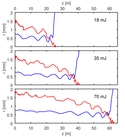
Figure 4: Boundary of 98% ionization (red lines) and $R_{1/2}(z)$ of the laser beam (blue lines) vs. propagation distance $z$ for three values of the incident pulse energy $E_{0}$. The horizontal axis has the same scale on all three panels.

These general features are valid for pulses of higher energy as demonstrated by Fig.4, which depicts the same plot (ion channel radius and $R_{1/2}$ vs. propagation distance) for three different initial pulse energies $E_{0}$. The fact that the trailing part of the pulse propagates in the transparent plasma channel almost unchanged can be seen of Fig. 5 where the temporal evolution of the pulse power (spatially integrated intensity) at several values of the propagation distance are plotted for two values of the initial pulse energy. The pulses are not attenuated homogeneously, energy is absorbed mostly around the leading edge (until full ionization is achieved). The leading edge steepens, while the trailing edge remains almost unchanged.

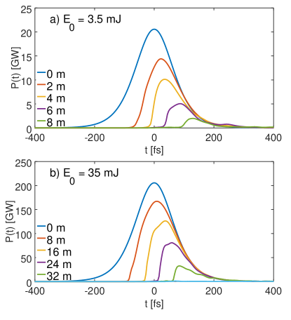
Figure 5: Time evolution of the pulse power at several positions along the propagation for two values of the initial energy a) $E_{0}=3.5\mathrm{~{}mJ}$ and b) $E_{0}=35\mathrm{~{}mJ}$.

III.2 Plasma channel properties

For the purposes of wakefield accelerator devices, the longitudinal and transverse extent of the plasma channel is of great importance, as is plasma homogeneity –the channel must be continuous, sufficiently wide with very close to 100% ionization. It can be seen on Fig. 4 that while the channel radius fluctuates considerably as the pulse propagates, there is also a clear tendency of gradual narrowing until the pulse “crashes”, i.e. the plasma channel radius becomes zero and the pulse intensity decreases below the level required for close to full ionization. Almost until this point the channel is uninterrupted, continuous and has a radius of $\sim$ 1 mm.

To make a more quantitative comparison, the evolution of the plasma channel has been calculated for a large number of initial pulse energies and the channel radius (radius of 98% ionization probability) plotted as a function of the energy $E(z)$ still left in the pulse after propagating a distance $z$. Some plots can be seen on Fig. 6, panel a). (The x axis of the plot has been reversed so that the pulses “propagate” from left to right similar to the rest of the figures in the paper.) It is clear that the average radius of the plasma channel as well as the magnitude of the fluctuations around it are the same for pulses that possess the same energy during their propagation at their respective propagation distances. Only the “phase” of these quasi-periodic oscillations differ. The channels end rather abruptly close to $E(z)=0$ in a very similar manner in all three cases.

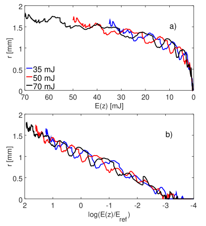
Figure 6: a) Plasma channel radius (boundary of 98% ionization probability) as a function of the energy still contained in the pulse for three different values of initial pulse energy $E_{0}$, 35 mJ, 50 mJ and 70 mJ. b) Plasma channel radius as a function of $\log(E(z)/E_{ref})$. The reference energy is $E_{ref}=10\mathrm{~{}mJ}$.

The same quantity (98% ionization probability radius) is plotted in Fig. 6 panel b) as a function of $\log(E(z)/E_{ref})$ where we have taken $E_{ref}=10\mathrm{~{}mJ}$ as a reference. This shows that the average channel radius is linear in this quantity, all three curves oscillate around the same line to a very good approximation. In fact, a linear fit to the curves $r(x)=mx+r_{0}$ (where $x$ stands for $\log(E/E_{ref}$) yields very similar values: $m=0.298\pm 0.005\mathrm{~{}mm}$ and $r_{0}=1.062\pm 0.003\mathrm{~{}mm}$ when averaged over 9 calculations with $E_{0}$ values between $16\mathrm{~{}mJ}-70\mathrm{~{}mJ}$. This suggests that there is a global attractor to the behavior of the propagating pulse that is independent of the initial pulse energy in the domain investigated. Repeating the calculations with a different beam waist parameter ($d=2\mathrm{~{}mm}$ initial beam diameter) we obtain a similar behavior, but different parameters for the line of best fit for the $r$ vs. $\log(E(z)/E_{ref})$ curves, namely $m=0.350\pm 0.007\mathrm{~{}mm}$. This indicates that though there is a globally attracting behavior also in this case, this is quantitatively different from the one for $d=1.5\mathrm{~{}mm}$, i.e. initial beam focusing has a long-term effect on the propagation.

For our purposes, we will now define the length of the plasma channel $L$ as the propagation distance at which the on-axis ionization probability drops below 98% for the first time. With this definition, the channel length is strictly zero for pulses that fail to ionize 98% of the atoms at $z=0$, even if self-focusing increases on-axis intensity to create a channel after some propagation length. Clearly, $L$ will depend on the initial pulse energy and focusing (among other parameters) and, due to the nature of the radius curve with quasi-periodic oscillations, this quantity too will oscillate somewhat. Plotting $L$ as a function of the initial pulse energy for two different values of the initial laser beam diameter (Fig. 7) shows that there is indeed a long-term effect of the initial focusing on the propagation. The difference between the two curves increases with $E_{0}$ which would not be the expected behavior if, after some initial transient the pulse propagation tended to the same attractor solution for both beam diameters.

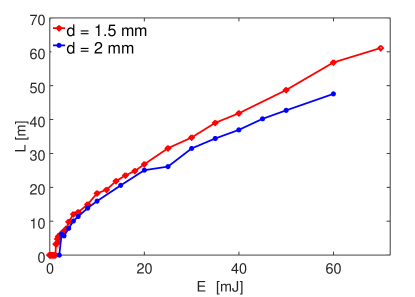
Figure 7: Plasma channel length as a function of initial pulse energy $L(E_{0})$ for two values of the initial beam diameter.

III.3 Effects of initial focusing

To investigate the effect of initial beam focusing, a set of calculations with constant $E_{0}$ but different $d$ was performed. Figure 8 depicts a curve of the plasma channel length for $E_{0}=8\mathrm{~{}mJ}$ pulses as a function of $d$ (red line). The curve is not strictly monotonous, because the plasma channel length as defined above may change abruptly when, for certain parameters there is a small dip in the on-axis ionization probability close to the end of the pulse propagation before a revival of the ionization probability. However there is a clear maximum at $d=0.8\mathrm{~{}mm}$ and the channel length is a fraction of the maximum value when $d$ is much smaller or much larger than optimal. Two insets on Fig. 8 depict a contour plot of the ionization probability for two sub-optimal values of the initial beam diameter and reveal the reason for this behavior. When the initial focusing is too tight (inset (a) ), the Rayleigh range is small and diffraction causes the beam to expand and ionize in a larger radius around the axis, depleting the energy severely. When the initial spot size is too large on the other hand (inset (b) ), the initial channel radius is large and a lot of energy is lost before the beam contracts to a more modest size. An additional feature visible on the plots are the “holes” in the ionization profile, small localized domains where ionization is not perfect, plasma density is inhomogeneous within the channel. Therefore a good choice of initial focusing also proves to be important for realizing homogeneous, long plasma channels for plasma wave acceleration.

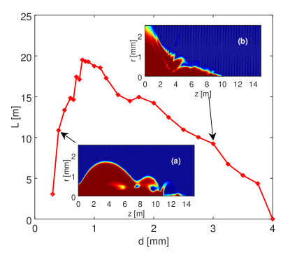
Figure 8: Main plot: Plasma channel length as a function of initial beam diameter $L(d)$ for a $E_{0}=8\mathrm{~{}mJ}$ pulse. Inset (a): contour plot of ionization probability as a function of radial distance $r$ and propagation distance $z$ for $d=0.4\mathrm{~{}mm}$. Inset (b): contour plot of ionization probability for $d=3\mathrm{~{}mm}$.

IV Some further comments

The model for the optical response of the atoms presented in this paper contains numerous approximations, trying to capture resonant interaction and ionization simultaneously and, at the same time, to be lightweight enough for extended propagation calculations in two spatial dimensions. In experiments and calculations of laser pulse filamentation in atmospheric gases it was observed that for sufficiently large values of the pulse power (several times the critical power $P_{cr}$ required for the onset of self-focusing and filamentation), a transverse instability breaks axial symmetry, the beam breaks up into multiple filaments Bespalov and Talanov (1966); Kandidov et al. (2005); Alonso et al. (2010); Champeaux and Bergé (2005); Rohwetter et al. (2008); Champeaux et al. (2008). Our axially symmetric description naturally excludes obtaining such solutions. While not immediately obvious whether multifilamentation can appear in a resonant system, this means that our model may overestimate the plasma channel length for a given vapor density and laser focusing.

The fact that the laser can resonantly transfer atoms to excited states has an effect on the ionization process as well. Analysis of the numerical solution shows that the onset of ionization is less abrupt, it starts at lower intensities than without resonance. The reason is that apart from three-photon ionization from the ground state, a process of resonant excitation followed by two-photon ionization, and a process of resonant excitation twice followed by single-photon ionization is also possible. In fact during the initial part of the propagation, before the pulse leading edge steepens too much, the dominant route to ionization is the one by two-photon absorption from the first excited state.

Initial derivation of the theory included an electron current term $\sim\partial J/\partial t$ that describes plasma absorption and dispersion. However, after verifying that this term has a very little effect in calculations presented in the paper, the term was neglected while performing extended parameter scans. This might be surprising at first, because in general, plasma density gradients are a major source of defocusing processes in laser pulse filamentation. However, in our case: i) because of full ionization the existence of plasma density gradients is limited to a narrow boundary region around the channel core, (in the center the plasma is completely homogeneous,) and most of the energy carried by the pulse is channeled in the transparent central part. ii) the vapor density is so low that even with full ionization, plasma is orders of magnitude less dense than in normal filamentation scenarios. Thus the fact that this term should have a negligible effect on the shape and extension of the plasma channel is understandable. Under different conditions, (e.g. much higher vapor densities or possibly much longer propagation lengths) the effects of the plasma term would be non-negligible.

Interaction of the laser pulse with the ionic core of the singly ionized rubidium has also been neglected completely in the present description. This is justified by the fact that the vapor is too rare for the usual, nonresonant optical coefficients to be effective and that the ionization potential is an order of magnitude greater than that for the valence electron of rubidium.

The phenomena discussed in this paper should not be termed “filamentation” as it is understood in the usual sense. Filamentation in that sense occurs when there is an (almost) lossless Kerr medium to self-focus the beam and an abrupt onset of absorption due to multiphoton ionization. An ionization potential much larger than the photon energy ($E_{i}\gg\hbar\omega$) is required for this Couairon and Mysyrowicz (2007) and the beam collapses to a transverse size $\sim 100{\mathrm{\mu}m}$. In the present case absorption is always present except when the medium is saturated and the transverse size of the beam remains about an order of magnitude larger as the focusing nonlinearity is also saturable. This width is already sufficient for application in accelerator devices such as AWAKE.

V Summary

We have investigated the propagation of ultra-short, ionizing laser pulses in rubidium vapor under conditions of direct single-photon resonance with an atomic transition from the ground state. To make the problem tractable for numerical solution in two spatial dimensions, we developed a relatively lightweight theory that includes the nonlinear response of atoms to resonant fields to all orders. Ionization was inserted in the theory as a phenomenological probability loss from the atomic levels. A split-step quasi-spectral method was used to solve a first order propagation equation in frequency space in the slowly-evolving wave approximation.

The dynamics of self-focusing, plasma channel formation and pulse collapse due to energy depletion were studied using parameter scans of computer simulations. We have shown that given sufficient pulse energy, a competition between nonlinear self-focusing and diffraction results in the pulse energy being confined in a narrow region around the propagation axis. The front part of the propagating pulse ionizes atoms close to the axis and so a plasma channel is formed with almost complete ionization of the rubidium vapor. The energy of the trailing part of the pulse is guided along the channel which is essentially transparent for the field. The radius of the plasma channel exhibits quasi-periodic oscillations around an average value which in turn is determined by the energy remaining in the pulse at the given propagation distance. Initial pulse focusing has a long-term effect on propagation, the average channel radius is different for pulses with different initial beam widths even at large propagation distances. The dependence of the plasma channel length on initial pulse energy and beam diameter has been studied. The calculations are expected to be useful for considerations in wakefield accelerator devices where the creation of homogeneous, spatially extended, dense plasmas are necessary, such as at the AWAKE project at CERN.

Appendix A Material parameters of the theory

We use the following notation to identify atomic states in the equations:

$$|5S_{1/2},m=1/2\rangle \rightarrow|1\rangle$$

$$|5P_{3/2},m=1/2\rangle \rightarrow|2\rangle$$

$$|5D_{3/2},m=1/2\rangle \rightarrow|3\rangle$$

$$|5D_{5/2},m=1/2\rangle \rightarrow|4\rangle$$

The energy levels of the excited states relative to the $|1\rangle$ ground state are Kramida et al. (2018): $\hbar\omega_{2}=1.589049\mathrm{~{}eV}$, $\hbar\omega_{3}=3.1864603\mathrm{~{}eV}$, $\hbar\omega_{4}=3.1868276\mathrm{~{}eV}$. Given that the photon energy for 780 nm light is 1.5895 eV, three photons are required for ionization from $|1\rangle$, two photons from $|2\rangle$ and a single photon from $|3\rangle$ and $|4\rangle$. The dipole matrix elements between the states are obtained from Steck (2009) and Safronova et al. (2004) and transformed to the conventions used in Steck (2016):

$$\langle 1|\hat{d}|2\rangle= 5.9786\cdot\mathrm{e\cdot a_{0}}\cdot\sqrt{1/4}\sqrt{2/3}$$

$$\langle 2|\hat{d}|3\rangle= 0.787\cdot\mathrm{e\cdot a_{0}}\cdot\sqrt{1/4}\cdot\sqrt{1/15}$$

$$\langle 2|\hat{d}|4\rangle= 2.334\cdot\mathrm{e\cdot a_{0}}\cdot\sqrt{1/6}\cdot\sqrt{3/5}$$

For the (intensity dependent) multiphoton ionization rates $\Gamma_{1},\Gamma_{2}$ from the ground and first excited states we use the well known PPT formulas Perelomov et al. (1966, 1967); Perelomov and Popov (1967). They are written using the notations of Béjot (2008), and are reproduced below from Eqs. 1.25-1.30 on pages 19-21 of Béjot (2008) for reference. The full formula for the ionization rate of any atom from a quantum state characterized by $l$ and $m_{l}$ is:

$$W(\omega_{0},\gamma)= \omega_{a.u.}\sqrt{\frac{6}{\pi}}|C_{n^{*},l^{*}}|^{2}f(l,m_{l})\frac{U_{i}}{2U_{H}}A_{m_{l}}(\omega_{0},\gamma)$$ (11)

$$\times\left(\frac{2E_{0}}{E\sqrt{1+\gamma^{2}}}\right)^{2n-|m_{l}|-3/2}\mathrm{exp}\left[-\frac{2E_{0}}{3E}g(\gamma)\right]$$

In this formula $\gamma$ is the famous Keldysh parameter

$$\omega_{0}\frac{\sqrt{2m_{e}U_{i}}}{|eE_{max}|}$$ (12)

with $U_{i}$ being the ionization energy, $U_{i}=4.177128\mathrm{~{}eV}$ for the $\mathrm{5S_{1/2}}$ state and $U_{i}=2.588079\mathrm{~{}eV}$ for the $\mathrm{5P_{3/2}}$ state. $m_{e}$ is the electron mass and $E_{max}$ is the maximum field amplitude. In LABEL:ionrate $U_{H}$ is the ionization energy of hydrogen, $\omega_{a.u.}=eE_{H}/\sqrt{2m_{e}U_{H}}\simeq 4.1\cdot 10^{16}\mathrm{~{}s^{-1}}$, $E_{H}=e^{5}m_{e}^{2}/(64\hbar^{4}\pi^{3}\epsilon_{0}^{3})\simeq 501.4\mathrm{~{}GV/m}$, $E_{0}=E_{H}(U_{i}/U_{H})^{3/2}$. The factor

$$|C_{n^{*},l^{*}}|^{2}=\frac{2^{2n^{*}}}{n^{*}\Gamma(n^{*}+l^{*}+1)\Gamma(n^{*}-l^{*})}$$ (13)

contains the effective quantum numbers $n^{*}$ which is $n^{*}=\sqrt{U_{H}/U_{i}}$ for $Z=1$, and $l^{*}=n^{*}-1$, $\Gamma()$ is the gamma function here. The rest of the factors in LABEL:ionrate are:

$$f(l,m_{l})= \frac{(2l+1)(l+|m_{l}|)!}{2^{|m_{l}|}(|m_{l}|)!(l-|m_{l}|)!}$$ (14)

$$A_{m_{l}}(\omega_{0},\gamma)= \frac{4\gamma^{2}}{\sqrt{3\pi}|m_{l}|!(1+\gamma^{2})}$$

$$\times\sum_{K\geq\nu}^{\infty}e^{-\alpha(K-\nu)}\Phi_{m_{l}}\left(\sqrt{\beta(K-\nu)}\right)$$

$$\Phi_{m_{l}}(x)= e^{-x^{2}}\int_{0}^{x}(x^{2}-y^{2})^{|m_{l}|}e^{y^{2}}dy$$

$$\beta(\gamma)= \frac{2\gamma}{\sqrt{1+\gamma^{2}}}$$

$$\alpha(\gamma)= 2\mathrm{sinh}^{-1}(\gamma)-\beta(\gamma)$$

$$g(\gamma)= \frac{3}{2\gamma}\left[\left(1+\frac{1}{2\gamma^{2}}\right)\mathrm{sinh}^{-1}(\gamma)-\frac{\sqrt{1+\gamma^{2}}}{2\gamma}\right]$$

$$\nu_{0}= \frac{U_{i}}{\hbar\omega_{0}}$$

$$\nu= \nu_{0}\left(1+\frac{1}{2\gamma^{2}}\right)$$

The ionization rates calculated from Eq. LABEL:ionrate are used as $\Gamma_{1}$ and $\Gamma_{2}$ in Eqs. 5 and 8. The single photon ionization rate $\Gamma_{4}$ was calculated using the experimental cross-section $\sigma=10.9\mathrm{~{}Mb}$ from Duncan et al. (2001), which has been measured for $\lambda=788\mathrm{~{}nm}$ light. The same value was used for $\Gamma_{3}$.

References

- Bergé (1998) L. Bergé, Physics Reports 303, 259 (1998).
- Couairon and Mysyrowicz (2007) A. Couairon and A. Mysyrowicz, Physics Reports 441, 47 (2007).
- Bergé et al. (2007) L. Bergé, S. Skupin, R. Nuter, J. Kasparian, and J.-P. Wolf, Reports on Progress in Physics 70, 1633 (2007).
- Kandidov et al. (2009) V. P. Kandidov, S. A. Shlenov, and O. G. Kosareva, Quantum Electronics 39, 205 (2009).
- Kolesik and Moloney (2013) M. Kolesik and J. V. Moloney, Reports on Progress in Physics 77, 016401 (2013).
- Caldwell et al. (2016) A. Caldwell et al., Nuclear Instruments and Methods in Physics Research Section A: Accelerators, Spectrometers, Detectors and Associated Equipment 829, 3 (2016), 2nd European Advanced Accelerator Concepts Workshop - EAAC 2015.
- Gschwendtner et al. (2016) E. Gschwendtner et al., Nuclear Instruments and Methods in Physics Research Section A: Accelerators, Spectrometers, Detectors and Associated Equipment 829, 76 (2016), 2nd European Advanced Accelerator Concepts Workshop - EAAC 2015.
- Adli et al. (2018) E. Adli, A. Ahuja, O. Apsimon, R. Apsimon, A.-M. Bachmann, D. Barrientos, F. Batsch, J. Bauche, V. B. Olsen, M. Bernardini, et al., Nature 561, 363 (2018).
- Doussot et al. (2016) J. Doussot, P. Béjot, and O. Faucher, Phys. Rev. A 94, 013805 (2016).
- Doussot et al. (2017) J. Doussot, G. Karras, F. Billard, P. Béjot, and O. Faucher, Optica 4, 764 (2017).
- Boshier and Sandle (1982) M. G. Boshier and W. J. Sandle, Optics Communications 42, 371 (1982).
- LAMB (1971) G. L. LAMB, Rev. Mod. Phys. 43, 99 (1971).
- de Lamare et al. (1994) J. de Lamare, M. Comte, and P. Kupecek, Phys. Rev. A 50, 3366 (1994).
- Delagnes and Bouchene (2008) J. Delagnes and M. Bouchene, Optics Communications 281, 5824 (2008).
- Fill (1994) E. E. Fill, J. Opt. Soc. Am. B 11, 2241 (1994).
- Brabec and Krausz (1997) T. Brabec and F. Krausz, Phys. Rev. Lett. 78, 3282 (1997).
- Couairon et al. (2011) A. Couairon, E. Brambilla, T. Corti, D. Majus, O. de J. Ramírez-Góngora, and M. Kolesik, The European Physical Journal Special Topics 199, 5 (2011).
- Steck (2009) D. A. Steck, Rubidium 85 D Line Data (available online at http://steck.us/alkalidata, (revision 2.1.2, 12 August 2009)).
- Kramida et al. (2018) A. Kramida, Y. Ralchenko, J. Reader, and N. A. Team, NIST Atomic Spectra Database (National Institute of Standards and Technology, Gaithersburg, MD., 2018).
- Safronova et al. (2004) M. S. Safronova, C. J. Williams, and C. W. Clark, Phys. Rev. A 69, 022509 (2004).
- Perelomov et al. (1966) A. M. Perelomov, V. S. Popov, and M. V. Terent’ev, Soviet Physics JETP 23, 924 (1966).
- Perelomov et al. (1967) A. M. Perelomov, V. S. Popov, and M. V. Terent’ev, Soviet Physics JETP 24, 207 (1967).
- Perelomov and Popov (1967) A. M. Perelomov and V. S. Popov, Soviet Physics JETP 25, 336 (1967).
- Kelley (1965) P. L. Kelley, Phys. Rev. Lett. 15, 1005 (1965).
- Marburger (1975) J. H. Marburger, Progress in Quantum Electronics 4, 35 (1975).
- Fibich et al. (2005) G. Fibich, S. Eisenmann, B. Ilan, Y. Erlich, M. Fraenkel, Z. Henis, A. L. Gaeta, and A. Zigler, Opt. Express 13, 5897 (2005).
- Feit and Fleck (1974) M. D. Feit and J. A. Fleck, Applied Physics Letters 24, 169 (1974).
- Couairon (2003) A. Couairon, Phys. Rev. A 68, 015801 (2003).
- Béjot et al. (2011) P. Béjot, E. Hertz, J. Kasparian, B. Lavorel, J. P. Wolf, and O. Faucher, Phys. Rev. Lett. 106, 243902 (2011).
- Courvoisier et al. (2003) F. Courvoisier, V. Boutou, J. Kasparian, E. Salmon, G. Méjean, J. Yu, and J.-P. Wolf, Applied Physics Letters 83, 213 (2003).
- Kolesik and Moloney (2004) M. Kolesik and J. V. Moloney, Opt. Lett. 29, 590 (2004).
- Skupin et al. (2004) S. Skupin, L. Bergé, U. Peschel, and F. Lederer, Phys. Rev. Lett. 93, 023901 (2004).
- Bespalov and Talanov (1966) V. I. Bespalov and V. I. Talanov, Soviet Journal of Experimental and Theoretical Physics Letters 3, 307 (1966).
- Kandidov et al. (2005) V. Kandidov, N. Akozbek, M. Scalora, O. Kosareva, A. Nyakk, Q. Luo, S. Hosseini, and S. Chin, Applied Physics B 80, 267 (2005).
- Alonso et al. (2010) B. Alonso, A. Zaïr, J. S. Román, O. Varela, and L. Roso, Opt. Express 18, 15467 (2010).
- Champeaux and Bergé (2005) S. Champeaux and L. Bergé, Phys. Rev. E 71, 046604 (2005).
- Rohwetter et al. (2008) P. Rohwetter, M. Queißer, K. Stelmaszczyk, M. Fechner, and L. Wöste, Phys. Rev. A 77, 013812 (2008).
- Champeaux et al. (2008) S. Champeaux, L. Bergé, D. Gordon, A. Ting, J. Peñano, and P. Sprangle, Phys. Rev. E 77, 036406 (2008).
- Eaton et al. (2017) J. W. Eaton, D. Bateman, S. Hauberg, and R. Wehbring, GNU Octave version 4.2.1 manual: a high-level interactive language for numerical computations (2017).
- Steck (2016) D. A. Steck, Quantum and Atom Optics (available online at http://steck.us/teaching, (revision 0.10.3, 13 April 2016)).
- Béjot (2008) P. Béjot, Theoretical and experimental investigations of ultrashort laser filamentation in gases, Ph.D. thesis (2008), , Université de Genève 2008 https://archive-ouverte.unige.ch/unige:4568.
- Duncan et al. (2001) B. C. Duncan, V. Sanchez-Villicana, P. L. Gould, and H. R. Sadeghpour, Phys. Rev. A 63, 043411 (2001).